Lattice Boltzmann Methodsfor Fluid Dynamics

Steven OrszagDepartment of Mathematics

Yale University

In collaboration with Hudong Chen, IsaacGoldhirsch, and Rick Shock

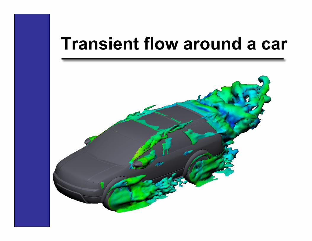
Transient flow around a car

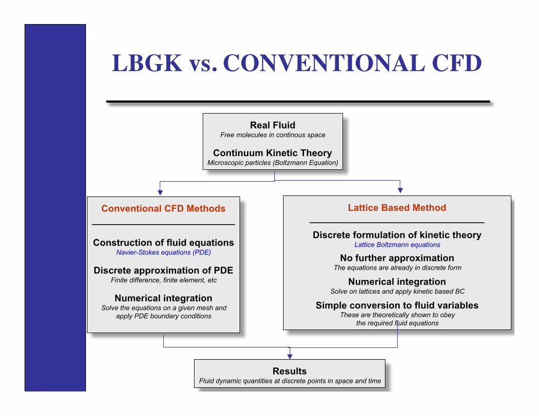
LBGK vs. CONVENTIONAL CFD

Real FluidFree molecules in continous space

Continuum Kinetic TheoryMicroscopic particles (Boltzmann Equation)

Conventional CFD Methods___________________________

Construction of fluid equationsNavier-Stokes equations (PDE)

Discrete approximation of PDEFinite difference, finite element, etc

Numerical integrationSolve the equations on a given mesh and

apply PDE boundary conditions

Lattice Based Method_________________________________

Discrete formulation of kinetic theoryLattice Boltzmann equations

No further approximationThe equations are already in discrete form

Numerical integrationSolve on lattices and apply kinetic based BC

Simple conversion to fluid variablesThese are theoretically shown to obey

the required fluid equations

ResultsFluid dynamic quantities at discrete points in space and time

0

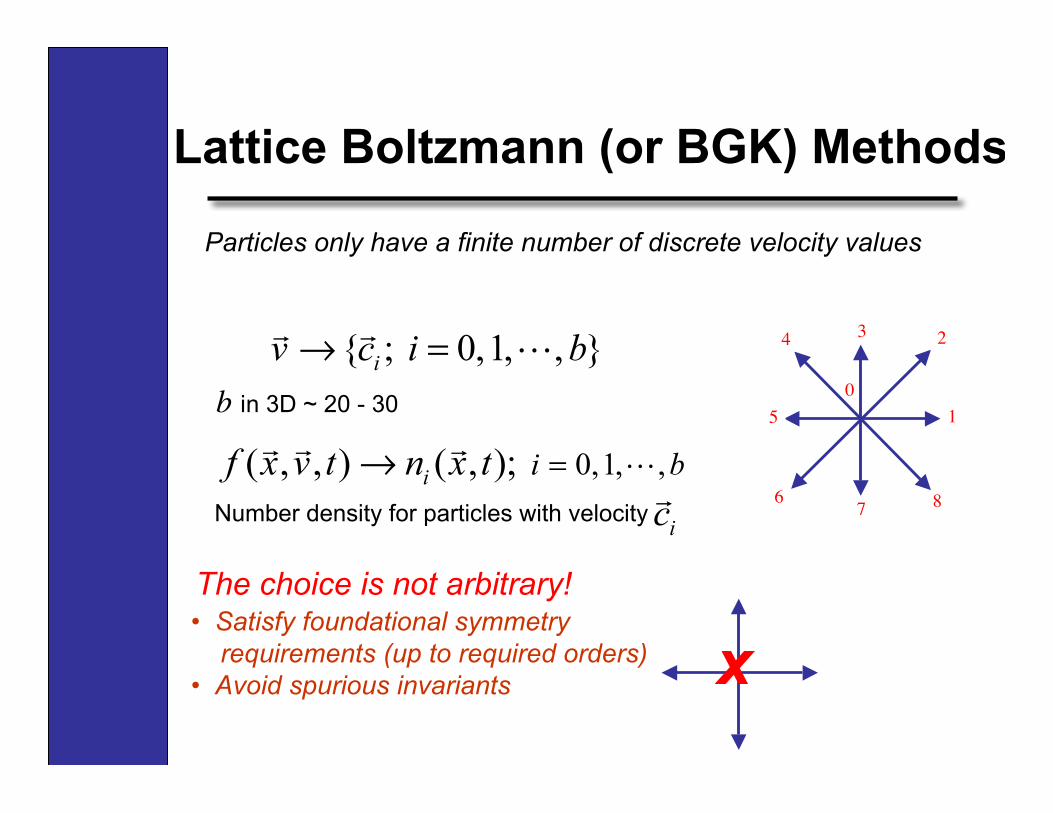
Lattice Boltzmann (or BGK) Methods

8

Particles only have a finite number of discrete velocity values

{ ; 0,1, , }i

v c i b! =! !

"

The choice is not arbitrary!• Satisfy foundational symmetry requirements (up to required orders)• Avoid spurious invariants

b in 3D ~ 20 - 30

2

1

34

5

6 7

x

0,1, ,( , , ) ( , );i i bf x v t n x t =! !" " "

Number density for particles with velocity ic!

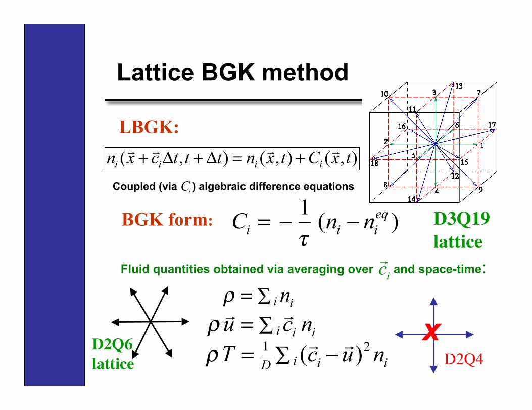
Lattice BGK method

LBGK:

Coupled (via ) algebraic difference equationsiC

BGK form:

Fluid quantities obtained via averaging over and space-time:

( , ) ( , ) ( , )i i i in x c t t t n x t C x t+ ! + ! = +! ! ! !

1( )eqi i iC n n

!= " "

i in! "=

i i iu c n! "=! !

1 2( )i i iDT c u n! "= #

! !

ic!

D3Q19lattice

xD2Q4

D2Q6lattice

Remarks on LBGK• Lattice BGK yields the Navier-Stokes equations

• Chapman-Enskog asymptotic expansion in powers of Knudsen number λ/L or τ/T << 1

• Easy to compute time dependent flows

• Relaxation time τ defines viscosity

• No need to compute pressure explicitly

• Boundary conditions are fully realizable

• Stability is ensured

• Parallel performance with arbitrary geometry

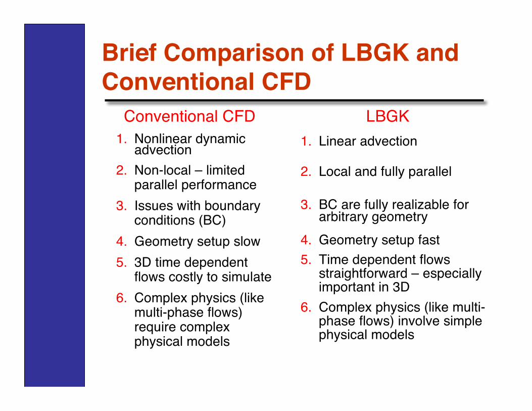
Brief Comparison of LBGK andConventional CFD

1. Nonlinear dynamicadvection

2. Non-local – limitedparallel performance

3. Issues with boundaryconditions (BC)

4. Geometry setup slow5. 3D time dependent

flows costly to simulate6. Complex physics (like

multi-phase flows)require complexphysical models

1. Linear advection

2. Local and fully parallel

3. BC are fully realizable forarbitrary geometry

4. Geometry setup fast5. Time dependent flows

straightforward – especiallyimportant in 3D

6. Complex physics (like multi-phase flows) involve simplephysical models

Conventional CFD LBGK

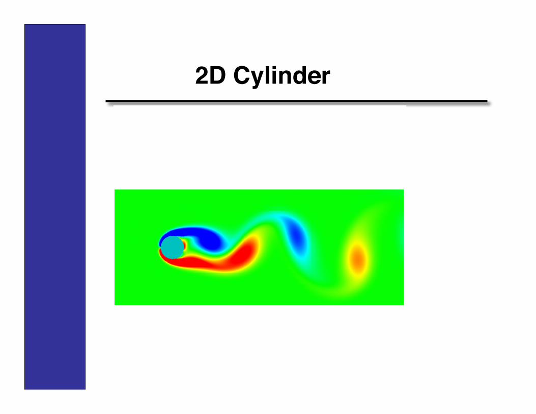
2D Cylinder

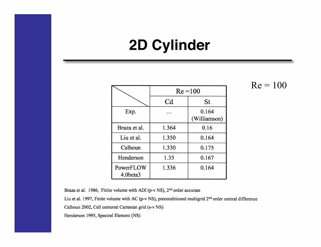
Re = 100

2D Cylinder

Friction Drag

2D Cylinder

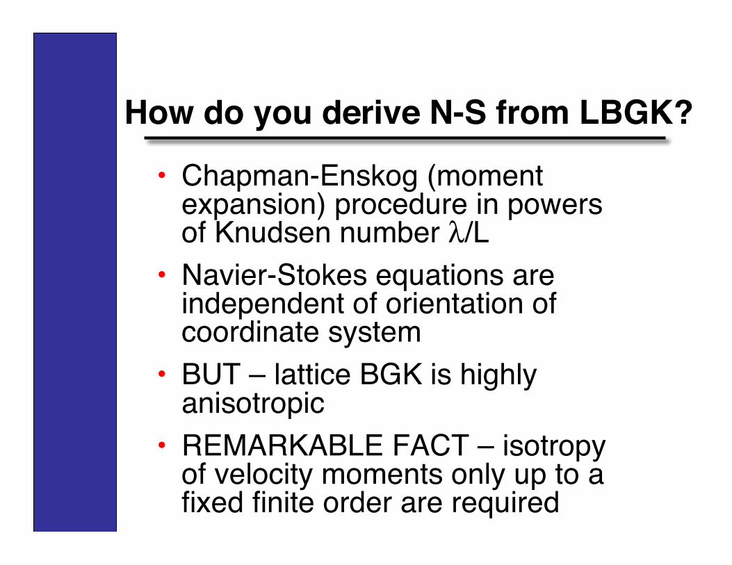
How do you derive N-S from LBGK?

• Chapman-Enskog (momentexpansion) procedure in powersof Knudsen number λ/L

• Navier-Stokes equations areindependent of orientation ofcoordinate system

• BUT – lattice BGK is highlyanisotropic

• REMARKABLE FACT – isotropyof velocity moments only up to afixed finite order are required

Isothermal Navier-Stokes equationsat low Mach numbers

• Density/momentum

• Momentum flux tensor

• Energy flux tensor

• Navier-Stokes requires isotropy ofvelocity moments only up to 4th order

1 1

( ) ( ) ( ) ( )b b

t f t t f t! ! !! !

" "= =

, # , , , # ,$ $x x u x c x

1

( ) ( )b

ij i jP t c c f t

! ! !

!

, ,

=

, " ,#x x

1

( ) ( )b

ijk i j kQ t c c c f t

! ! ! !

!

, , ,

=

, " ,#x x

High-order models• Non-isothermal low Mach number Navier-

Stokes equations requires velocitymoment isotropy up to 6th order

• Other physically relevant models reuqireeven higher-order velocity momentisotropy, further restricting the discretevelocity set used in lattice BGK

• For example, non-isothermal flow withBurnett corrections requires 8th orderisotropy

Relation between rotational symmetryand order of moment isotropy in 2D

• b velocitiesis invariant under rotations by multiples of 2π/b

• Isotropy of the nth order basis moment tensor

requires that where A is a constant and is any unit vector• This requires that be

independent of θ, which holds ifie (2j-n)/b is not a nonzero integer for j=0,…,n

• CONCLUSION: Isotropy for sohexagonal lattice gives 4th order isotropy, etc.

( )

b

n

n

! ! !

!

" #M c c c!!!!!!

ˆ( )

b

nv A

!

!

" =# c

2 2{ ( ( ) ( ) 0 1}C cos sin … b

b b!

"! "!!= = , ; = , , #c

ˆ ( )v cos sin! != , 1( )

0

2( ) ( )

b

n n

bh cos

b!

"!# #

$

=

% $& 21

(2 )

0

0b

bi j ne

!"

"

##

=

=$

2n b! "

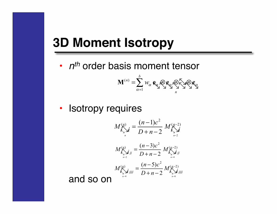
3D Moment Isotropy• nth order basis moment tensor

• Isotropy requires

and so on

( )

1

b

n

n

w ! ! ! !

!=

= " " "#M c c c!!!!!!!!

! !2

2( ) ( 2)( 1)

2n n

n nn cM M

i i i iD n

!

!!=

+ !! !

! !2 4

2( ) ( 2)( 3)

2n n

n n

jj jj

n cM M

i i i iD n! !

!!=

+ !! !

! !4 6

2( ) ( 2)( 5)

2n n

n n

jjjj jjjj

n cM Mi i i iD n

! !

!!=

+ !! !

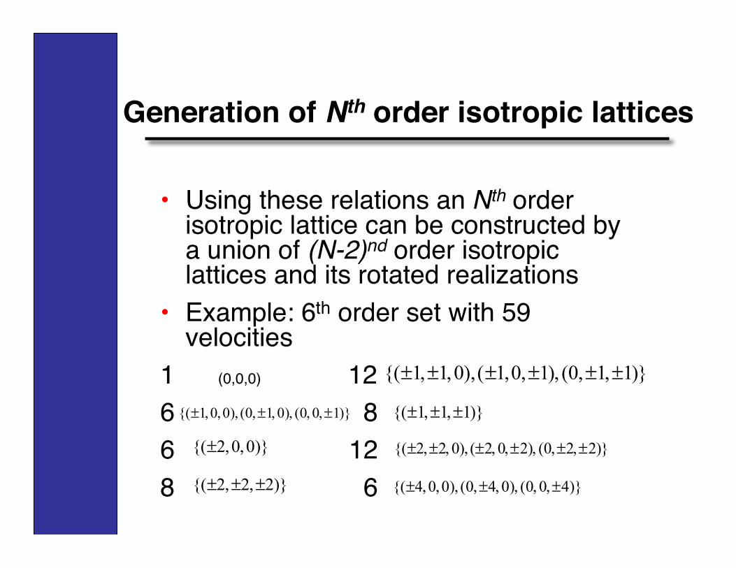
Generation of Nth order isotropic lattices

• Using these relations an Nth orderisotropic lattice can be constructed bya union of (N-2)nd order isotropiclattices and its rotated realizations

• Example: 6th order set with 59velocities

1 (0,0,0) 126 86 128 6

{( 1 1 0) ( 1 0 1) (0 1 1)} ± ,± , , ± , ,± , ,± ,±

{( 1 0 0) (0 1 0) (0 0 1)} ± , , , ,± , , , ,± {( 1 1 1)} ± ,± ,±

{( 2 0 0)} ± , , {( 2 2 0) ( 2 0 2) (0 2 2)} ± ,± , , ± , ,± , ,± ,±

{( 2 2 2)} ± ,± ,± {( 4 0 0) (0 4 0) (0 0 4)} ± , , , ,± , , , ,±

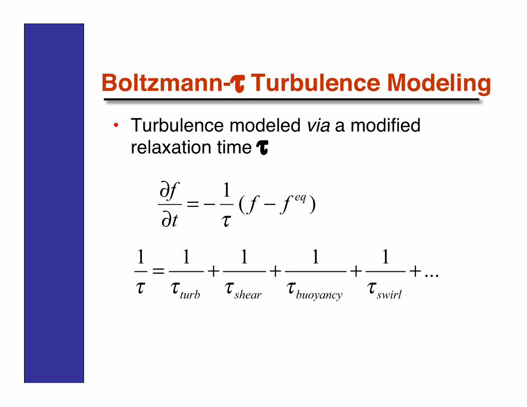
Boltzmann-τ Turbulence Modeling• Turbulence modeled via a modified

relaxation time τ

)(1 eqff

t

f!!=

"

"

#

1 1 1 1 1...

turb shear buoyancy swirl! ! ! ! != + + + +

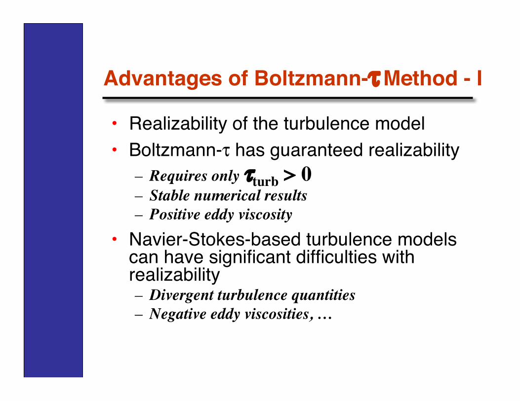
Advantages of Boltzmann-τ Method - I

• Realizability of the turbulence model• Boltzmann-τ has guaranteed realizability

– Requires only τturb > 0– Stable numerical results– Positive eddy viscosity

• Navier-Stokes-based turbulence modelscan have significant difficulties withrealizability– Divergent turbulence quantities– Negative eddy viscosities, …

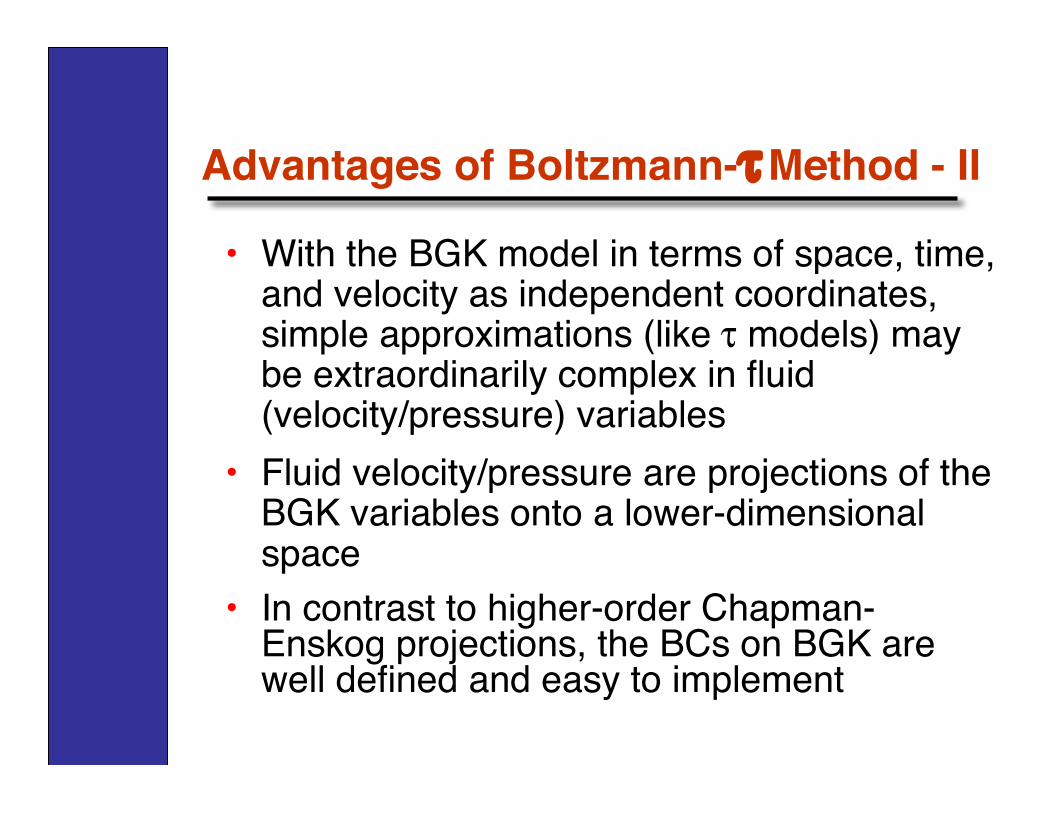
Advantages of Boltzmann-τ Method - II

• With the BGK model in terms of space, time,and velocity as independent coordinates,simple approximations (like τ models) maybe extraordinarily complex in fluid(velocity/pressure) variables

• Fluid velocity/pressure are projections of theBGK variables onto a lower-dimensionalspace

• In contrast to higher-order Chapman-Enskog projections, the BCs on BGK arewell defined and easy to implement

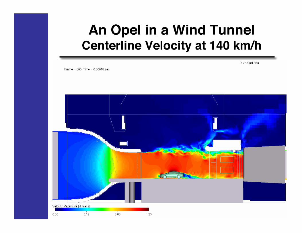
An Opel in a Wind TunnelCenterline Velocity at 140 km/h

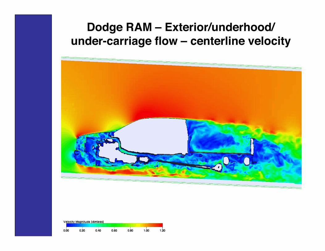
Dodge RAM – Exterior/underhood/under-carriage flow – centerline velocity

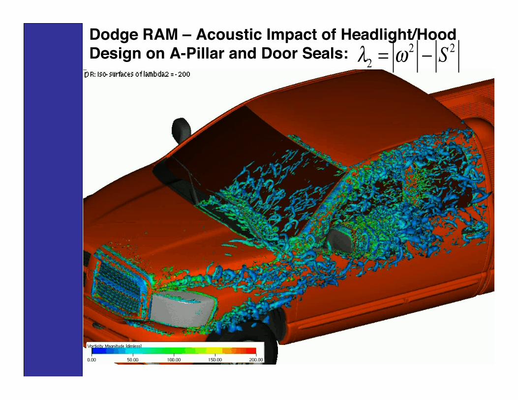
Dodge RAM – Acoustic Impact of Headlight/HoodDesign on A-Pillar and Door Seals: 2 2

2S! "= #

3D Streamlines of Flow Past aLarge Truck

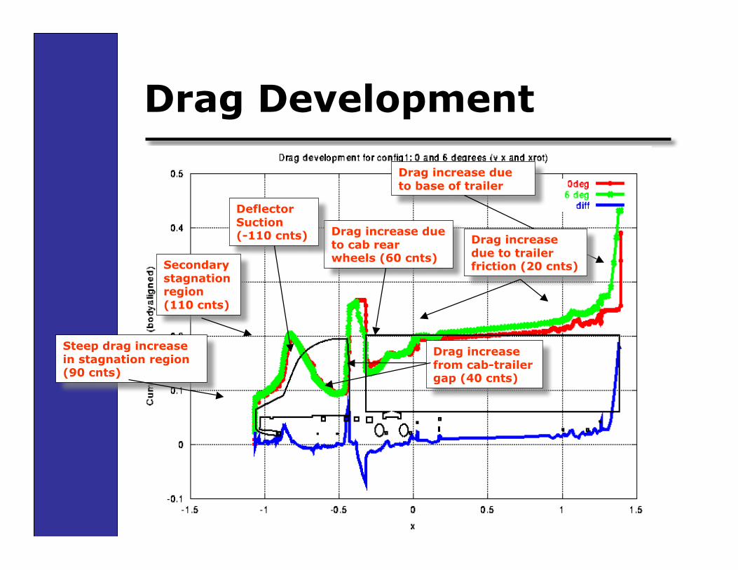
Drag Development

Steep drag increasein stagnation region(90 cnts)

Drag increase dueto cab rearwheels (60 cnts)

DeflectorSuction(-110 cnts)

Drag increase dueto base of trailer

Secondarystagnationregion(110 cnts)

Drag increasefrom cab-trailergap (40 cnts)

Drag increasedue to trailerfriction (20 cnts)

Conclusions• Lattice BGK allows straightforward

mix of complex fluids, complexphysics, and complex geometries

• Appropriate lattice structures can bederived to assure accurate andefficient flow computations, evenwith turbulence and other complexphysics included