late quaternary geomorphology of arroyos in …
TRANSCRIPT
LATE QUATERNARY GEOMORPHOLOGY OF ARROYOS IN THE MIXTECA ALTA,
OAXACA, MEXICO
by
Genevieve A. Holdridge
(Under the Direction of David S. Leigh)
ABSTRACT
Land degradation in drylands is one of the most critical, ongoing global environmental
issues, and gullying and arroyos constitute some of the more serious elements of desertification.
The overarching goal was to examine how late Quaternary climate, land use, and environmental
change influenced the dryland stream dynamics of the Río Culebra watershed, located in the
semi-arid Mixteca Alta in southwestern Mexico. This goal was examined through three separate,
but interrelated studies. The first study (Chapter 2) examined the sediment yield and land use of
the dryland fluvial system of the Río Culebra watershed. Conservative bedload yield estimates
on two tributary arroyos demonstrated that despite headwater conservation, the yield is still
relatively high, and suggest the need for larger scale conservation efforts. Present channel bed
stratigraphy containing predominantly massive, coarser deposits contrasts the prevalence of finer
bedded sediments in the Quaternary stratigraphy, which indicate a different flood regime in the
past. The second study (Chapter 3) concerned the uncertainty of the relative contributions of
anthropogenic versus climatic drivers on land degradation. The alluvium-paleosol chronology
was examined against regional climatic conditions and indicated that greater incision occurred

during wetter periods, while alluvial deposition and paleosol formation occurred during
transitional wet and dry periods, supporting the “wet-dry-wet” model of arroyo cycles.
Comparing the paleoclimatic-paleohydrological relationship of terminal Pleistocene and early
Holocene strata versus the late Holocene strata indicated that widepsread agricultural activities
greatly impacted sediment rates and influenced the timing and nature of landscape response to
climate change. The third study (Chapter 4) addressed the need for better understanding the
local paleoenvironment. The local paleoenvironment, as reflected in soil organic matter δ13C
values and paleosol data is comparable to the paleoclimatic and paleoenvironmental
reconstruction from central and southwestern Mexico. The paleoenvironment of Culebra
watershed was impacted by lama-bordo (i.e., check dam) and agricultural terrace constructions
and the increased importance of maize cultivation and succulent plant managment during the late
Holocene. The results of these studies illustrate the need to understand long-term climatic,
hydrologic and land use variability in order to find solutions to dryland desertification in the
present.
INDEX WORDS: Quaternary stratigraphy, Arroyo cycles, Sediment yield, Erosion, Land
use, Paleohydrology, Incision, Agradation, Semi-arid, Dryland streams,
Stable carbon isotopes, Check dams, Mixteca Alta, Mexico
LATE QUATERNARY GEOMORPHOLOGY OF ARROYOS IN THE MIXTECA ALTA,
OAXACA, MEXICO
by
GENEVIEVE A. HOLDRIDGE
BA, University at Albany-SUNY, 2001
MS, Bilkent University, Turkey, 2004
MPhil, University of Cambridge, United Kingdom, 2006
A Dissertation Submitted to the Graduate Faculty of The University of Georgia in Partial
Fulfillment of the Requirements for the Degree
DOCTOR OF PHILOSOPHY
ATHENS, GEORGIA
2016

© 2016
Genevieve A. Holdridge
All Rights Reserved

LATE QUATERNARY GEOMORPHOLOGY OF ARROYOS IN THE MIXTECA ALTA,
OAXACA, MEXICO
by
GENEVIEVE A. HOLDRIDGE
Major Professor: David S. Leigh
Committee: George A. Brook
L. Bruce Railsback
David F. Porinchu
Electronic Version Approved:
Suzanne Barbour
Dean of the Graduate School
The University of Georgia
August 2016

iv
“Nothing is softer or more flexible than water,
yet nothing can resist it.”
-Lao Tzu

v
ACKNOWLEDGEMENTS
Thanks to various sources of funding, I was able to complete my dissertation including
the following: the Fulbright Garcia-Robles (2012-2013); the Geologic Society of America Grant
(2013); the USAID Small Projects Grant (2014); and the Summer Dissertation Write-up Grant
UGA (2016). Also thanks to my opportunity as a Peace Corps Response Volunteer, I was able to
work on part of my project for an extra year as well as work with many local communities in the
Mixteca Alta.
There are many people to thank as I could not have achieved this PhD without their help,
support, insight and experience. Firstly, I would like to thank the administraters of many
municipalities in the Coixtlahuaca District for giving me permission and support to conduct my
work. In particular, I would like to thank the municipalities of San Juan Bautista Coixtlahuaca
and Santa Maria Nativitas and the administrators therein. I would like to thank colleagues at the
Biosphere Reserve for their enormous support with logistics in the field and their interest in my
project that resulted in my position as a Peace Corps Response Volunteer. Thanks to Rafael
Arzarte Aguirre, Roberto Navarro, Socorro Garcia, and Fernando Reyes, I learned so much about
the region, and was able to co-organize two foros in the Coixtlahuaca district. I am grateful to
the employees - my friends- at the Peace Corps including Heather Zissler, Beatriz Charles and
especially Angel Pineda, who was my director and helped me coordinate my new position and
logistics.
I would also like to thank the geoarchaeological team with whom I started my research in
Coixtlahuaca, in particular Gabby Garcia Ayala and Stefan Brannan. I am so greatful to the
vi
project´s co-director, Steve Kowalewski, who like another committee member, offered tons of
support and shared his expertise on the archaeology and anthropology of the region; this project
would never have been completed without his support.
Professors from other insitutions also offered their support such as lecturer Gerardo
Roman Gonzalez Rojas at the Institute of Tehuacan, who helped organize water quality analyses
from Coixtlahuaca, and Lorenzo Selem for insightful discussions (Geographer at the National
Autonomous University of Mexico (UNAM) in Mexico City. Also David Gale, (astrophysicist,
University of the Americas, Puebla) who was such a good friend – thanks for showing me the
Azteca! In particular, I would like to thank JP Bernal at UNAM (Geochemist, Queretaro
campus), also like another committee member, took me in as one of his students and included me
on his caving projects and stalagmite research. He offered much support despite my
unsuccessful attempt to incorporate stalagmite work into my dissertation (but not unsuccessful
for long….!). Thanks to him for all the insightful discussions about geochemistry,
geomorphology and archaeology, etc., - but most especially his friendship. Thanks to Julie
Hemple for letting me stay at her house in Queretaro and for teaching me about Mexican
literature, and thanks to the other students at UNAM (Queretaro campus) and my friends in the
group: los Musicos Queretaros!
I lived in Coixtlahauca for three years and have met so many wonderful people, including
Chavela Garcia Juarez and her family, thanks to them for the mezcals, dinners, and teaching me
so much about the local Oaxacan culture. I am grateful for the dinners with Regina and her
family, and Florinda and her family. Lucia, thank you for the interesting talks! Most especially I
would like to thank mi tía, Altagracia Garcia Lara, who is my adopted aunt, with whom I lived
with for almost 2 years, and with whom I have shared many meals and heartfelt talks. Her

vii
children and grandchildren, the rest of the Garcia Lara family, have shown so much support
while I lived in the village. In particular, I would like to recognize Blademir Victor Garcia Lara
who is very insightful, an engineer in his own right, and who has succeeded in conserving much
of his land in the headwaters of Sandage. He serves as a model for all of us. Thanks to Fidelia
Garcia Juarez (Victor´s wife) for her insight and support and their son Richy who has helped me
so much in the field. Finally, many other field and lab workers were employed by me, but Juan
Carlos Juerez Jimenez, Karen Betanzos and Berenice Lara were exceptional employees and I
could not have done this without them.
My lab work involved isotopes and I appreciate the support of Julia Cox in the Geology
Isotope Lab, and the scientists at the Center for Applied Isotopes: especially Doug Dvorocek and
Alex Cherkinsky. Much of my writing and map-making took place in the Center for Geospatial
Research, and I thank the the lab for its support (and safetly) in particular, Tommy Jordan,
Magarite Madden, Sergio Bernardes, David Cotten, Roberta Samli, and Brandon Adams. To my
fellow physical geographers, thanks for all the good discussions and the impetus to finish! In
particular Jake McDonald, Pete Akers and Lixin Wang. To other friends who have enriched my
life and opend my mind, especially Brooke Tave, Guy Savir, Mike and Alicia Coughlan, Tiffany
Videl, Shadrock Roberts, Megan Westbrook, Peter Baas, Megan MacMuller, Isaac Lungu and
Mohammed Yaffa.
Thanks to my committee, firstly David Porinchu for his critical and insightful comments.
I am so grateful to Bruce Railsback, who taught me so much and helped me achieve something
with my undateable stalagmites. Thanks to George Brook (best soccer player), as I have learned
so much from him and who has given much support over the years. I would have never made it
without his help, and dare I say friendship! Finally, to my advisor David Leigh, thanks for

viii
believing in me. It has been tough as I have been in the field so much. Thanks to David for all
of his insight, knowledge, guidance and support. I have learned so much from him - from field
methods to better writing. I am so happy we worked together. Salud!
To Stuart and Laina Swiny, thanks for all the support over the years. They are like
family to me and my life would have not been the same if I had not attended that excavation on
Cyprus with them all those years ago (2001)! To all my family, thank you so much for being
there for me! In particular, I would like to thank my Aunt and Uncle, Ruth Harman and Jack
Holdridge, who live in Athens. We have become so close, and thanks to them for sticking with
me through the ups and downs. I will never forget it and will always be there for them. Thanks
to my parents, Louise and Jim Holdridge, who have been behind me, pushed me, and who have
never given up on me. Also, I am grateful to my father, an excellent writer and editor, who did
last minute edits on my dissertation writing. I love you all!

ix
TABLE OF CONTENTS
Page
ACKNOWLEDGEMENTS .............................................................................................................v
LIST OF TABLES ........................................................................................................................ xii
LIST OF FIGURES ..................................................................................................................... xiii
CHAPTER
1 INTRODUCTION .........................................................................................................1
1.1 Overview and Objectives ...................................................................................1
1.2 Rationale ............................................................................................................3
1.3 Summary ............................................................................................................8
1.4 References ..........................................................................................................9
2 GEOMORPHIC CHARACTERISTICS AND BEDLOAD YIELD ESTIMATES OF
A DRYLAND STREAM SYSTEM IN SOUTHWESTERN MEXICO .....................17
2.1 Introduction and Objectives .............................................................................19
2.2 Study Area ......................................................................................................24
2.3 Methods............................................................................................................26
2.4 Results and Discussion ....................................................................................31
x
2.5 Conclusion .......................................................................................................48
2.6 References ........................................................................................................50
3 LATE PLEISTOCENE ARROYO CYCLES OF THE MIXTECA ALTA, OAXACA,
MEXICO ......................................................................................................................80
3.1 Introduction ......................................................................................................82
3.2 Study Area .......................................................................................................85
3.3 Methods............................................................................................................89
3.4 Results ..............................................................................................................93
3,5 Discussion ......................................................................................................105
3.6 Conclusion .....................................................................................................120
3.7 References .....................................................................................................121
4 STABLE CARBON ISOTOPE ANALYSIS OF PALEOSOL ORGANIC MATTER
IN THE MIXTECA ALTA, OAXACA, MEXICO ...................................................143
4.1 Introduction ....................................................................................................145
4.2 Study Area .....................................................................................................150
4.3 Methods..........................................................................................................152
4.4 Results ............................................................................................................158
4.5 Discussion ......................................................................................................163
4.6 Conclusion .....................................................................................................179
4.7 References ......................................................................................................181
5 CONCLUSION ..........................................................................................................209
5.1 Introduction ....................................................................................................209
5.2 Climate and Hydrology: Long-Term Variability ...........................................210
xi
5.3 Anthropogenic Drivers...................................................................................214
5.4 Epilogue .........................................................................................................215
5.5 References ......................................................................................................217
APPENDICES
I FLOOD AND BEDLOAD DATA ............................................................................220
II PROFILE DESCRIPTIONS AND ANALYSIS ........................................................226
III SUMMED PROBABILITY PLOTS AND AGE CALIBRATION ..........................283

xii
LIST OF TABLES
Page
Table 1.1: Characteristics of Drylands ...........................................................................................15
Table 2.1: Land cover classification for Barrancas Sandage and Sauce ........................................76
Table 2:2 Scour-and-fill information for Barrancas Sandage and Sauce for the flood season of
2013-2014 ..........................................................................................................................77
Table 2.3 Bedload and flow characteristics for Barranca Sandage during the flood seasons of
2013 and 2014 ....................................................................................................................78
Table 2.4 Bedload and flow characteristics for Barranca Sauce during the flood seasons of 2013
and 2014 .............................................................................................................................79
Table 3.1: Cultural phases of the Mixteca Alta . ………. ..........................................................139
Table 3:2 Radiocarbon dates from study area ..............................................................................140
Table 4.1 Results of the δ13C values analyses .............................................................................201
Table 4.2 The resulting modern δ13C values after applying correction for the Suess effect .......205
Table 4.3 The modern δ13C values used to calculate %C4 and CAM .........................................205
Table 4.4 Calculated precentages %C4 and CAM .......................................................................206

xiii
LIST OF FIGURES
Page
Figure 1.1: The Langbein-Schumm curve .....................................................................................15
Figure 2.1: Map of the Rio Culebra watershed and its tributaries in Oaxaca, Mexico ..................58
Figure 2.2: Google Earth satellite imagery of Barrancas Sauce and Sandaage .............................59
Figure 2.3: Example of modern check dam (e.g., Victor’s lama-bordos). ..................................60
Figure 2.4: Intact and blown-out ancient check dam in the headwaters of Barranca Sandage ......61
Figure 2.5: Monitoring station of Barranca Sandage .....................................................................62
Figure 2.6: Monitoring station of Barranca Sauce. ........................................................................63
Figure 2.7: Artificial knickpoint created by a bridge on Sandage .................................................64
Figure 2.8: Natural Knickpoints in the Rio Culebra Watershed ....................................................65
Figure 2.9: Examples of mass wasting. .........................................................................................66
Figure 2.10 Bed topography and morphology in Barrancas Sandage and Sauce. .........................67
Figure 2.11: Channel bed particle size distribution in Barrancas Sandage and Sauce. .................68
Figure 2.12: Distribution of channel bed material and shape of Barrancas Sandage and Sauce ...69
Figure 2.13: Scour-and-fill stratigraphy of the scouring chains in Barrancas Sandage and
Sauce…. .............................................................................................................................70
Figure 2.14: Quaternary alluvial stratigraphy in the Rio Culebra watershed ................................71
Figure 2.15: Particle size distribution for each flood in Sandage between 2013 and 2014 ...........72
Figure 2.16: Estimated bedload flux against maximum discharge for Sandage and Sauce for each
flood between 2013-2014 ..................................................................................................73

xiv
Figure 2.17: Estimated bedload flux values for Barrancas Sandage and Sauce against streams
from other environments ....................................................................................................74
Figure 2.18: Estimated bedload yield in tonnes per day for Barrancas Sandage and Sauce against
streams from other environments……...………………………...……………………….75
Figure 2.19: Estimaion of backfilling behind ancient and modern check dams ..........................129
Figure 3.1: Map of study area ………………………………………………………………….130
Figure 3.2: Map of settlement locations in the Rio Culebra valley from the Cruz and Natividad
phases …………………………………………………………………………………..131
Figure 3.3: Fence diagram of study profiles ................................................................................132
Figure 3.4: View of Profile C2…………………………………………………………………133
Figure 3.5: Stratigraphy and lama-bordo at S5…………………………………………………134
Figure 3.6: Results from LOI, weathering indices and horizon thickness analyses …. ..............135
Figure 3.7 Modeled sedimentation rates (cm/yr) for the Rio Culebra watershed ........................136
Figure 3.8 Results from the qualitative analyses .........................................................................137
Figure 3.9: Close-up of results from the qualitative analyses ......................................................138
Figure 3.10: Model of arroyo cycles in the Mixteca Alta ............................................................139
Figure 4.1: Map of study area ......................................................................................................191
Figure 4.2: Land cover map of the region ....................................................................................192
Figure 4.3: Relationship between depth and %TOC and δ13C ...................................................193
Figure 4.4: Distribution of δ13C values from the Culebra, Verde and Inguiro watersheds .........194
Figure 4.5: Variation of all δ13C values from the Culebra, Inguiro and Verde watersheds from the
terminal Pleistocene through the late Holocene. ...........................................................195
Figure 4.6: Local polynomial regression of the main trend of the δ13C values over time ...........196

xv
Figure 4.7 Summary of climate data in central and southwestern Mexico for the last 16,000
years…………………………………………………………………………………….197
Figure 4.8 Summary of climate data in central and southwestern Mexico for the last 16,000
years…………………………………………………………………………………….199

1
CHAPTER 1
INTRODUCTION
1.1 Overview and Objectives
Land degradation in drylands is identified as one of the most critical, ongoing global
environmental issues by the United Nations (UN Report, 2011). Drylands are defined as regions
that have an aridity index of between 0.03-0.75 (Table 1.1) (UN Report, 2011). Drylands cover
approximately 40% of the Earth’s land surface, and contain around 30% of the world’s
population (UN Report, 2011). Land degradation is defined as the damage to land productivity
in drylands that results from unsustainable land use practices and recent climate change (Annan,
2006; UN Report, 2011). Drylands, especially semi-arid and arid environments, are
characterized by rainfall variability and unstable hydrological regimes, leaving them particularly
vulnerable to land degradation (Sivakumar, 2007). Gullying and arroyo formation are types of
soil erosion that constitute one of the more serious elements of desertification, causing severe
damage to terrestrial and aquatic ecosystems (Dregne, 2002).
Notwithstanding the importance of other external factors (i.e., tectonics and base level),
the degree to which humans versus climate influence gullying and arroyo formation has been one
of the most prominent debates in geomorphology since the early 20th century. A study by Waters
and Haynes (2001) demonstrated that climate change alone generates arroyos, while land use
effects (e.g., cultivation, deforestation) on soil erosion and gullying have also been confirmed as
drivers by a number of studies (Walling, 1999; Knox, 2001; Poesen et al., 2003; Gellis et al.,

2
2004; Walling and Collins, 2008; Svoray and Markovitch, 2009). Geoarchaeological and
geomorphological research also supports that prehistoric land use practices, such as agriculture
and deforestation as well as population pressures and land abandonment, resulted in land
degradation during the late Holocene (Butzer, 1992; Denevan, 1992; O’Hara et al., 1993; Waters
and Ravesloot, 2000; McAuliffe et al., 2001; Fisher et al., 2003; Wilkinson, 2005a; Butzer et al.,
2008).
Although the overarching link between climate change, human activities, and
desertification is well documented for the last century (Karl and Trenberth, 2003; Giurma et al.,
2008), the relative contributions of anthropogenic versus climatic factors are unclear. This
uncertainty calls for more studies on the long-term climatic variability, land use change, and
related hydrologic responses in drylands (Poesen et al., 2003; Benito et al, 2010).
Research Objectives: This research focuses on late Quaternary arroyo processes, forms,
and functions in the semi-arid environment of the Río Culebra Valley, located in the Mixteca
Alta of southwestern Mexico. The overarching goal is to examine past and present dryland
stream dynamics in relation to climatic, land use, and environmental change. Although drylands
cover hyper-arid to sub-humid climates, in this research the term drylands in relation to the
Mixteca Alta will refer to a semi-arid environment, and the term ‘all drylands’ will denote the
entire ensemble of dryland environments. Three research objectives will be addressed in three
separate, but interrelated chapters, as follows:
Research Objective 1 (RO1): to study the channel bed morphology, bedload and
flow characteristics of the present ephemeral stream system in order to better understand
erosion in the region, as well as offer insight on interpreting the alluvial stratigraphy;
Chapter 2 provides data and interpretations related to this objective;
3
Research Objective 2 (RO2): to determine the relationship between paleoclimatic
fluctuations and arroyo formation prior to widespread agriculture in the region, and
compare the results from the pre-agricultural stratigraphy to the late prehistoric and
modern agricultural time periods in order to better discern the influences of climate
versus anthropogenic drivers; Chapter 3 provides data and interpretations related to this
objective;
Research Objective 3 (RO3): to examine paleoenvironmental change represented
by stable carbon isotopes in soil organic matter, and along with the paleoclimate
information provided by paleosols, to establish how the site specific record of
paleoenvironmental change corresponds with regional paleoenvironmental and
paleoclimatic fluctuations; Chapter 4 provides data and interpretations related to this
objective.
1.2 Rationale
According to Graf (1979) the term ‘arroyo’ was first used in the southwestern United
States by Dodge (1902), who defined them as: ‘steep-walled, flat-floored trenches excavated in
valley floors”. In some literature gullies denote smaller incised channels and are located in the
headwaters, while arroyos represent larger incised channels and are situated in valley bottoms,
but in other studies they are synonymous (as they will be used here) (Goudie, 2013). The terms
gullies and arroyos are also referred to as ephemeral streams, dryland rivers (Bull and Kirkby,
2002), and barrancas (local name in Oaxaca, Mexico), but the latter three terms typically refer to
continuous channels, whereas gullies and arroyos can be continuous or discontinuous (Bull,
1997). Flow in arroyos is usually ephemeral, but occasionally they contain perennial (i.e., when

4
supplied by a spring) or intermittent groundwater inflow (Bull, 1997; Goudie, 2013).
Additionally, in some regions arroyos undergo cycles of incision and aggradation, though it is
uncertain why they form and how they operate. The dryland streams in the study area are
continuous arroyos, having mainly ephemeral flow, but some streams are spring-fed perennial
streams and all demonstrate cycles of erosion and incision. To clarify, in this research ‘dryland
streams’ in the context of the Mixteca Alta will represent semi-arid dryland streams, but when
referring to all dryland streams the term ‘all dryland streams’ will be used.
Present arroyo formation has been linked to various combinations of climate-independent
(i.e., drainage area and morphometry, geology, slope, surficial crusts), climate-dependent (i.e.,
rainfall and temperature, flood frequency and magnitude, vegetation type and amount), and
anthropogenic causes (i.e., grazing, overpopulation, agriculture) (Jansson, 1988; Bull, 1991;
Bull, 1997; McFadden and McAuliffe, 1997; Hereford, 2002; Poesen et al., 2003; Avni, 2005;
Valentin et al., 2005; Jones et al., 2010). The combination of factors varies at times and for
different locations making it difficult to understand and predict arroyo formation. Internal
factors are important, as sensitive lithologies will produce higher amounts of sediment yield in
comparison to basins with more resistant lithologies with the same climate and land use
(McFadden and McAuliffe, 1997).
The overarching climatic and anthropogenic drivers and their relative contributions
toward arroyo formation are still uncertain (e.g., Boardman et al., 2010; Goudie, 2013). While
the connection between gully formation and climate, without human intervention, has been
substantiated (Waters and Haynes, 2001), contradictory hypotheses concerning arroyo formation
still endure (e.g., Borejsza et al., 2008; Solleiro-Rebolledo et al., 2011). Some studies maintain
that incision occurs during wet periods and alluviation in dry periods (Waters and Haynes, 2001;

5
Hereford, 2002), while others support base level control (i.e., dry periods cause base level to fall
and vice versa) (e.g., Haynes, 1968). In other cases, it has been argued that changes in intensity,
magnitude and frequency of precipitation regimes can affect arroyo cycles instead of adhering to
more general ‘wet’ and ‘dry’ terms (Leopold, 1976; Butzer et al., 2008; Huckleberry et al.,
2013). Arroyo cycles have been associated with climatic fluctuations on various time scales,
such as increasing ENSO intensity during the late Holocene (Waters and Haynes, 2001) and
millennial scale fluctuations associated with the strength of the North American Monsoon on a
‘1,500-year cycle’ (Mann and Meltzer, 2007). However, neither study indicates the precise
nature of how these large-scale climatic fluctuations would affect flood and sediment
characteristics. Rainfall associated with arroyo activity is characterized by high intensity and
low duration storms, when much sediment is eroded and transported from the catchment (Poesen
et al., 2003; Valentin et al., 2005); however, the present link between climatic drivers, such as
ENSO and rain intensity have not been clearly established.
Even though research has shown that gullying is a major contributor to erosion and
desertification in drylands, there are still many uncertainties concerning the effects that future
land use modifications will have on hydrologic responses for dryland streams (Poesen et al,
2003; Valentin et al., 2005; Sinha et al., 2012). Although the effects of various land use activities
on increased soil erosion and sedimentation have been well documented (e.g., Walling, 1999;
Wilkinson, 2005b; Walling and Collins, 2008), in many cases the severity and complexity of
local erosion are not well understood (Fox et al., 2016). Equally important is the need for more
understanding on how prehistoric land use and the accrual of land use over millennia influences
gullying. For example, some studies suggest that unsustainable agricultural practices during the
prehistoric periods in conjunction with a high population produced high rates of erosion (e.g.,

6
Melville, 1990; Butzer, 1992, O’Hara et al., 1993). Conversely, other studies have shown that
increased erosion was associated with land abandonment following a period of intensively well-
managed landscapes sustained by higher populations (e.g., Fisher et al., 2003; Redman, 2005).
Some studies on recently abandoned, terraced landscapes support the latter (Lesschen et al.,
2009), though conservation efforts have only recently been assessed (Polyavok et al., 2014).
Despite a limited understanding of the effects that climate change has on gullying without
human intervention, it has been argued that human activities have more severe impacts on arroyo
formation than climate change alone (e.g., Garcia-Ruiz, 2010). Teasing out human intervention
and/or climatic processes is very difficult in both the past and the present and confounded by the
fact that various climatic drivers can be reflected in similar fluvial responses, or equifinality
(Knox, 1993). Attaining a baseline of ‘natural’ responses of a basin to climatic events is essential
before attempting to assess how population fluctuations and land use activities affect landscape
response. Furthermore, the majority of research concerning the relationship between land
degradation and climate fluctuations concentrates on the last 200 years, neglecting to place this
within the context of both long-term climate variability and land use change (Mayewski et al.,
2004; Quigley et al., 2011). Deciphering the relationship between climate and arroyo cycles may
only be achieved by understanding both long- and short-term climatic fluctuations and landscape
response.
Research concerning the connection between human activities, climate change and
arroyos falls in line with studies of sediment erosion during the latter part of the 19th century into
the early part of the 20th century, many of which were made in the southwestern U.S. (Bryan,
1925; Bull, 1997). For instance, the Langbein-Schumm curve (Langbien and Schumm, 1958)
implies that semi-arid environments promote very high sediment yield, due to sufficient rain to

7
produce runoff, but insufficient rain to promote much vegetation growth (Figure 1.1). Although
it is clear that vegetation type and amount interacts with atmospheric and climatic conditions,
land use, and local factors to affect erosion (e.g., Abrahams et al., 1994), the relative contribution
of vegetation change as compared to extreme events in causing incision and aggradation has
been debated in recent studies (e.g., Antinao and McDonald, 2013; Pelletier, 2014). Vegetation
change both reflects overarching drivers and interacts with them to influence landscape response.
Therefore, incorporating several local and regional paleoclimatic and paleoenvironmental
proxies helps avoid equifinality while providing a more complete understanding of land use and
climate change.
Studies of process and form in relation to dryland streams have offered insight to aspects
of fluvial geomorphology such as hydrology, hydraulics, and channel sediments (Tooth, 2000).
Notions of thresholds and equilibrium have been exemplified through research on arroyo incision
and aggradation (Schumm and Hadley, 1957; Graf, 1979; Schumm, 1979). Studies on ephemeral
streams have shown that they contain a much higher amount of sediment load than perennial
counterparts (e.g., Laronne and Reid, 1993; Renard et al., 2008). It has been recognized that
much insight on Quaternary stratigraphy may be gained from examining present flood and
channel bed deposits to better understand stream behavior (Reid and Frostick, 1987; Reid, 2002;
Benvenuti et al., 2005; Billi, 2008). Despite some increased interdisciplinary discussion on
applying knowledge of obtained from short-term, process and form relationships in all present
dryland stream systems to better understand older sediments (Tooth, 2009), the application
toward better understanding the long-term hydrological conditions of the Quaternary still
requires attention. Investigations of semi-arid dryland alluvial flood deposits emphasize the
more erosive incision phase, while ignoring the aggradation phase (Benvenuti et al., 2005; Jones

8
et al 2010). This is partially due to the difficulty in contriving generalizations concerning the
alluvial sequences, which constitute a number of undated, discrete events (Harvey and Pederson,
2011). More reliance on present process-form relationships between sediment and flow may
alleviate these challenges by providing potential interpretations for sedimentary successions.
Conversely, in other areas like Mexico, the emphasis has been on paleosols with less
regard for the alluvium (Sedov et al., 2009; Solliero-Rebolledo et al., 2011). Paleosols indicate
either local or widespread landscape stability (Benvenuti et al., 2005; Solliero-Rebolledo et al.,
2011), but the intricacies of alluvial paleosol formation are often overlooked. Examining the
timing and characteristics of alluvial paleosols has the potential to offer valuable information
about the paleohydrology and alluvial stratigraphy of dryland stream systems (Aslan and Autin,
1998).
Additionally, examining the effects of climate change on near-surface processes will
provide a better understanding of the paleoclimatic fluctuations that affected similar stratigraphy
and features in the past (Kochel and Miller, 1997). Reid (2002) suggests that only large changes
will modify channel form and behavior in dryland streams, which may apply to some present,
dryland streams. Small changes in climate, however, can result in relatively large changes in
flood magnitude and frequency (Knox, 1993). Changes in internal dynamics and land use,
especially if widespread, may also produce threshold-crossing changes in dryland stream
behavior in conjunction with climate change.
1.3 Summary
Contradictory hypotheses concerning arroyo formation still endure because more studies
on paleosol-alluvium sequences are needed to connect paleoclimate drivers and paleohydrologic
9
responses before evaluating widespread land use change. In addition, more fluvial
geomorphological studies need to evaluate paleoenvironmental and paleoclimatic data against
paleosol-alluvial sequences. Our incomplete understanding of the natural variability of flood
characteristics and sediment yield in drylands is both due to the inadequate application of present
climate-hydrologic relationships to interpreting past alluvium as well as the lack of a long-term
perspective needed to more fully understand present systems. Finally, more research is needed
to understand the relationship between climate fluctuations, land use change and hydrologic
responses over the longue durée in order to untangle the interaction between desertification,
climate, and land use change in prehistoric to recent times. This dissertation seeks to contribute
to a better understanding of these complex issues.
1.4 References
Abrahams, A.D., Parsons, A.J., Wainwright, J., 1994. Resistance to Overland-Flow on Semiarid
Grassland and Shrubland Hillslopes, Walnut Gulch, Southern Arizona. Journal of
Hydrology 156, 431-446.
Annan, K., 2006. Protecting Drylands, Preventing Poverty, Deserts and Desertification: Don’t
Desert Drylands! Message of United Nations Secretary General, United Nations
Environment Programme Report, World Environment Day, http://www.unep.org/ -
wed/2006/downloads.PDF/WED2006Booklet_en.pdf. Last accessed January, 2015.
Antinao, J.L., McDonald, E., 2013. A reduced relevance of vegetation change for alluvial
aggradation in arid zones. Geology 41, 11-14.
Aslan, A., Autin, W.J., 1998. Holocene flood-plain soil formation in the southern lower
Mississippi Valley: Implications for interpreting alluvial paleosols. Geological Society of
America Bulletin 110, 433-449.
Avni, Y., 2005. Gully incision as a key factor in desertification in an and environment, the
Negev highlands, Israel. Catena 63, 185-220.
Benito, G., M. Rico, Y. Sanchez-Moya, A. Sopena, V. R. Thorndycraft, Barriendos, M., 2010.
10
The impact of late Holocene climatic variability and land use change on the flood
hydrology of the Guadalentin River, southeast Spain. Global and Planetary Change, 70,
53-63.
Billi, P., 2008. Bedforms and sediment transport processes in the ephemeral streams of Kobo
basin, Northern Ethiopia. Catena 75, 5-17.
Boardman, J., Foster, I., Rowntree, K., Mighall, T., Gates, J., 2010. Environmental Stress and
Landscape Recovery in a Semi-Arid Area, The Karoo, South Africa. Scottish
Geographical Journal 126, 64-75.
Borejsza, A., I. R. Lopez, C. D. Frederick, Bateman, M. D., 2008. Agricultural slope
management and soil erosion at La Laguna, Tlaxcala, Mexico. Journal of Archaeological
Science, 35, 1854-1866.
Bryan, K., 1925. Date of Channel Trenching (Arroyo Cutting) in the Arid Southwest. Science
(New York, N.Y.) 62, 338-344.
Bull, W.B., 1991. Geomorphic Responses to Climate Change. Oxford University Press, Oxford.
Bull, W.B., 1997. Discontinuous ephemeral streams. Geomorphology 19, 227-276.
Bull, L.J., Kirkby, M.J., 2002. Dryland River Characteristics and Concepts, in: Bull, L., J.,
Kirkby, M. J. (Ed.), Dryland Rivers: Hydrology and Geomorphology of Semi-Arid
Channels. John Wiley & Sons Ltd., West Sussex.
Butzer, K.W., 1992. The America Before and After 1492 – An Introduction to Current
Geographical Research. Annals of the Association of American Geographers 82, 345-
368.
Butzer, K.W., Abbott, J.T., Frederick, C.D., Lehman, P.H., Cordova, C.E., Oswald, J.F., 2008.
Soil-geomorphology and "wet" cycles in the Holocene record of North-Central Mexico.
Geomorphology 101, 237-277.
Denevan, W.M., 1992. The pristine myth: the landscape of the Americas in 1492. Annals of the
Association of American Geographers 82, 369-385.
Dregne, H. E., 2002. Land degradation in the drylands. Arid Land Research and Management,
16, 99-132.
Fisher, C. T., H. P. Pollard, I. Israde-Alcantara, V. H. Garduno-Monroy, Banerjee, S. K., 2003. A
reexamination of human-induced environmental change within the Lake Patzcuaro Basin,
Michoacan, Mexico. Proceedings of the National Academy of Sciences of the United
States of America, 100, 4957-4962.
Fox, G.A., Sheshukov, A., Cruse, R., Kolar, R.L., Guertault, L., Gesch, K.R., Dutnell, R.C.,
11
2016. Reservoir Sedimentation and Upstream Sediment Sources: Perspectives and Future
Research Needs on Streambank and Gully Erosion. Environmental Management 57, 945-
955.
García-Ruiz, J. M., 2010. The effects of land uses on soil erosion in Spain: A review. Catena,
81, 1-11.
Gellis, A.C., Pavich, M.J., Bierman, P.R., Clapp, E.M., Ellevein, A., Aby, S., 2004. Modern
sediment yield compared to geologic rates of sediment production in a semi-arid basin,
New Mexico: Assessing the human impact. Earth Surface Processes and Landforms 29,
1359-1372.
Graf, W., 1979. The Development of Montane Arroyos and Gullies. Earth Surface Processes and
Landforms 4, 1-14.
Giurma, I., C. R. Giurma-Handley, I. Craciun, Antohi, C. M., 2008. Global Dimming- An
Environmental Hypothesis on Climate Change. Environmental Engineering and
Management Journal, 7, 417-421.
Goudie, A. S., 2013. Arid and Semi-Arid Geomorphology. Cambridge: University of
Cambridge Press.
Harvey, J.E., Pederson, J.L., 2011. Reconciling arroyo cycle and paleoflood approaches to late
Holocene alluvial records in dryland streams. Quaternary Science Reviews 30, 855-866.
Haynes, C.V., Jr., 1968. Geochronology of late-Quaternary alluvium, in R.B. Morrison & H.E.
Wright, Jr. (Eds.), Means of correlation of Quaternary successions, 591–631, Salt Lake
City: University of Utah Press.
Hereford, R., 2002. Valley-fill alluviation during the Little Ice Age (ca. AD 1400-1880), Paria
River basin and southern Colorado Plateau, United States. Geological Society of America
Bulletin 114, 1550-1563.
Huckleberry, G., Duff, A.I., 2008. Alluvial cycles, climate, and puebloan settlement shifts near
Zuni Salt Lake, New Mexico, USA. Geoarchaeology-an International Journal 23, 107-
130.
Huckleberry, G., J. Onken, W. M. Graves, Wegener, R., 2013. Climatic, geomorphic, and
archaeological implications of a late Quaternary alluvial chronology for the lower Salt
River, Arizona, USA. Geomorphology, 185, 39-53.
Jansson, M.B., 1988. A Global Survey of Sediment Yield. Geografiska Annaler
Series a-Physical Geography 70, 81-98.
Jones, L. S., M. Rosenburg, M. D. Figueroa, K. McKee, B. Haravitch, Hunter, J., 2010.
12
Holocene valley-floor deposition and incision in a small drainage basin in western
Colorado, USA. Quaternary Research, 74, 199-206.
Karl, T. R., Trenberth, K. E., 2003. Modern global climate change. Science, 302, 1719-1723.
Knox, J.C., 1993. Large Increases in Flood Magnitude in Response to Modest Changes in
Climate. Nature 361, 430-432.
Knox, J. C., 2001. Agricultural influence on landscape sensitivity in the Upper Mississippi River
Valley. Catena, 42, 193-224.
Kochel, R. C., Miller, J. R., 1997. Geomorphic responses to short-term climatic change: An
introduction. Geomorphology, 19, 171-173.
Langbein, W.B., Schumm, S.A., 1958. Yield of sediment in relation to mean annual
precipitation. Trans Amer Geophys Union 39, 1076-1084.
Laronne, J.B., Reid, I., 1993. Very High-Rates of Bedload Sediment Transport by Ephemeral
Desert Rivers. Nature 366, 148-150.
Lesschen, J. P., J. M. Schoorl, Cammeraat, L. H., 2009. Modelling runoff and erosion for a
semi-arid catchment using a multi-scale approach based on hydrological connectivity.
Geomorphology, 109, 174-183.
Leopold, L. B., 1976. Reversal of Erosion Cycle and Climatic Change. Quaternary Research, 6,
557-562.
Mann, D.H., Meltzer, D.J., 2007. Millennial-scale dynamics of valley fills over the past 12,000
C-14 yr in northeastern New Mexico, USA. Geological Society of America Bulletin 119,
1433-1448.
Mayewski P.A., E.E. Rohling, J.C. Stager, K. Wibjörn, K. A. Maasch, L. D. Meeker, E. A.
Meyerson, F. Gasse, S. van Kreveld, K. Holmgren, J. Lee-Thorp, G. Rosqvist, F. Rack,
M. Staubwasser, R. R. Schneider, Steig, E. J., 2004. Holocene climate variability.
Quaternary Research, 62, 243-255.
McAuliffe, J.R., Sundt, P.C., Valiente-Banuet, A., Casas, A., Viveros, J.L., 2001. Pre-columbian
soil erosion, persistent ecological changes, and collapse of a subsistence agricultural
economy in the semi-arid Tehuacan Valley, Mexico's 'Cradle of Maize'. Journal of Arid
Environments 47, 47-75.
McFadden, L.D., McAuliffe, J.R., 1997. Lithologically influenced geomorphic responses to
Holocene climatic changes in the Southern Colorado Plateau, Arizona: A soil-
geomorphic and ecologic perspective. Geomorphology 19, 303-332.
Melville, E. G. K., 1990. Environmental and Social-Change in the Valle-del-Mezquital, Mexico,
13
1521-1600. Comparative Studies in Society and History, 32, 24-53.
O'Hara, S.L., Street-Perrott, F.A., Burt, T.P., 1993. Accelerated soil erosion around a Mexican
highland lake caused by prehispanic agriculture. Nature 362, 48-51.
Pelletier, J.D., 2014. The linkages among hillslope-vegetation changes, elevation, and the timing
of late-Quaternary fluvial-system aggradation in the Mojave Desert revisited. Earth
Surface Dynamics 2, 455-468.
Poesen, J., Nachtergaele, J., Verstraeten, G., Valentin, C., 2003. Gully erosion and
environmental change: importance and research needs. Catena 50, 91-133.
Polyakov, V.O., Nichols, M.H., McClaran, M.P., Nearing, M.A., 2014. Effect of check dams on
runoff, sediment yield, and retention on small semiarid watersheds. Journal of Soil and
Water Conservation 69, 414-421.
Quigley, M. C., T. Horton, J. C. Hellstrom, M. L. Cupper, Sandiford, M. 2010. Holocene climate
change in arid Australia from speleothem and alluvial records. Holocene, 20, 1093-1104.
Redman, C. L., 2005. Resilience theory in archaeology. American Anthropologist, 107, 70-77.
Reid, I., 2002. Sediment Dynamics of Ephemeral Channels, in: Bull, L.J., Kirkby, M.J. (Eds.),
Dryland Rivers: Hydrology and Geomorphology of Semi-Arid Channels. John Wiley &
Sons Ltd., Wests Sussex.
Reid, I., Frostick, L.E., 1987. Flow Dynamics and Suspended Sediment Properties in Arid Zone
Flash Dynamics and Suspended Sediment Properties in Arid Zone Flash Floods.
Hydrological Processes 1, 239-253.
Renard, K.G., Nichols, M.H., Woolhiser, D.A., Osborn, H.B., 2008. A brief background on the
U.S. Department of Agriculture - Agricultural Research Service Walnut Gulch
Experimental Watershed. Water Resources Research 44.
Schumm, S.A., Hadley, R.F., 1957. Arroyos and the Semiarid Cycle of Erosion. American
Journal of Science 255, 161-174.
Schumm, S. A. (1979) Geomorphic Thresholds - Concept and Its Applications. Transactions of
the Institute of British Geographers, 4, 485-515.
Sedov, S., Solleiro-Rebolledo, E., Terhorst, B., Sole, J., Flores-Delgadillo, M.D., Werner, G.,
Poetsch, T., 2009. The Tlaxcala basin paleosol sequence: a multiscale proxy of middle to
late Quaternary environmental change in central Mexico. Revista Mexicana De Ciencias
Geologicas 26, 448-465.
Sinha, R., Latrubesse, E.M., Nanson, G.C., 2012. Quaternary fluvial systems of tropics: Major
14
issues and status of research. Palaeogeography Palaeoclimatology Palaeoecology 356,1-
15.
Sivakumar, M. V. K., 2007. Interactions between climate and desertification. Agricultural and
Forest Meteorology, 142, 143-155.
Solleiro-Rebolledo, E., Sycheva, S., Sedov, S., McClung de Tapia, E., Rivera-Uria, Y., Salcido-
Berkovich, C., Kuznetsova, A., 2011. Fluvial processes and paleopedogenesis in the
Teotihuacan Valley, Mexico: Responses to late Quaternary environmental changes.
Quaternary International 233, 40-52.
Svoray, T., Markovitch, H., 2009. Catchment scale analysis of the effect of topography, tillage
direction and unpaved roads on ephemeral gully incision. Earth Surface Processes and
Landforms 34, 1970-1984.
Tooth, S., 2000. Process, form and change in dryland rivers: a review of recent research. Earth-
Science Reviews 51, 67-107.
UN, 2011. Global Drylands: A UN system-wide response. United Nations Environmental
Management Group.
Valentin, C., Poesen, J., Li, Y., 2005. Gully erosion: Impacts, factors and control. Catena 63,
132-153.
Walling, D.E., 1999. Linking land use, erosion and sediment yields in river basins.
Hydrobiologia 410, 223-240.
Walling, D.E., Collins, A.L., 2008. The catchment sediment budget as a management tool.
Environmental Science & Policy 11, 136-143.
Waters, M.R., Haynes, C.V., 2001. Late Quaternary arroyo formation and climate change in the
American Southwest. Geology 29, 399-402.
Waters, M.R., Ravesloot, J.C., 2001. Landscape change and the cultural evolution of the
Hohokam along the middle Gila River and other river valleys in south-central
Arizona. American Antiquity 66, 285-299.
Wilkinson, T.J., 2005a. Soil erosion and valley fills in the Yemen highlands and southern
Turkey: Integrating settlement, geoarchaeology, and climate change. Geoarchaeology- an
International Journal 20, 169-192.
Wilkinson, B.H., 2005b. Humans as geologic agents: A deep-time perspective. Geology
33, 161-164.
15
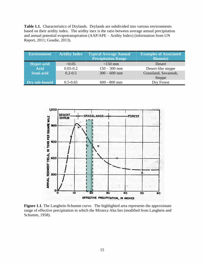
Table 1.1. Characteristics of Drylands. Drylands are subdivided into various environments
based on their aridity index. The aridity inex is the ratio between average annual precipitation
and annual potential evapotranspiration (AAP/APE – Aridity Index) (information from UN
Report, 2011; Goudie, 2013).
Environment Aridity Index Typical Average Annual
Precipitation Range
Examples of Associated
Biome(s)
Hyper-arid <0.05 <150 mm Desert
Arid 0.05-0.2 150 – 300 mm Desert-like steppe
Semi-arid 0.2-0.5 300 – 600 mm Grassland, Savannah,
Steppe
Dry sub-humid 0.5-0.65 600 - 800 mm Dry Forest
Figure 1.1. The Langbein-Schumm curve. The highlighted area represents the approximate
range of effective precipitation in which the Mixteca Alta lies (modified from Langbein and
Schumm, 1958).

16
CHAPTER 2
GEOMORPHIC CHARACTERISTICS AND BEDLOAD YIELD ESTIMATES OF A
DRYLAND EPHEMERAL STREAM IN SOUTHWESTERN MEXICO1
1 Holdridge, G. A. and Leigh, D. S. To be submitted to the International Journal of Sediment Research.

17
Abstract
Semi-arid dryland streams are known for their very high sediment loads, in particular
high bedload yields, resulting from widespread sediment availability and efficient transport.
Intense and sporadic rainfall, sparse vegetation cover, erodible geology, and land use change
contribute to land degradation. Semi-arid environments are especially vulnerable to widespread
erosion. Local communities and governmental agencies attempt to control gullying and arroyo
formation by applying various conservation strategies, including check dams. The effectiveness
of check dams on downstream sediment yield and geomorphology is still relatively unclear. The
dryland fluvial system of the Río Culebra watershed, located in the semi-arid region of the
Mixteca Alta, southwestern Mexico, was examined to better understand the present-day sediment
yield and check dam effectiveness, and to provide context for past sediment yield. It also offered
information concerning prehistoric agricultural landscape management.
A general survey of the watershed was undertaken to evaluate the processes and
morphology characterizing the present dryland stream system. A more in-depth study was made
on two tributary arroyos to the Culebra to estimate bedload yield and to gain a better
understanding of erosion in the region, as well as community efforts to reduce soil erosion. One
of the tributary arroyos, Barranca Sandage, contains soil conservation structures in the
headwaters that included modern construction of several sediment check dams. The other
arroyo, Barranca Sauce, is poorly managed and contains a high proportion of bare ground land
cover.
The geomorphic survey suggests that the entire watershed is undergoing internal
adjustments or complex response from legacy and recent land use impacts. Conservative
bedload yield estimates suggest that even with headwater conservation, the yield is still relatively
18
high, even during low flow conditions. Continued high bedload yield points to the need for
larger scale conservation efforts. The arroyo with more bare ground indicates that transmission
loss is also important and influences the bedload yield. Based on conservative estimates of
modern daily bedload yield of 17 tonnes in Barranca Sandage and 45 tonnes in Barranca Sauce,
the time it would take to fill ancient and modern check dams was calculated to be 23 and 249
years, respectively. The modern bedload sediment yield is at least 4.6 times greater than the
prehistoric sediment yield during the late Holocene, based on modeled sedimentation rates
associated with the ancient lama-bordos. The examination of present-day processes and forms
also offered insight to understanding and interpreting the alluvium-paleosol stratigraphy.
Present channel bed stratigraphy associated with scour-and-fill consists of poorly sorted,
massive, sandy gravel deposits. Finer bedded sediments are observed in the present patchy
floodplain deposits, but are susceptible to erosion. In contrast, the Quaternary stratigraphy is
dominated by extensive fine sediment deposits, having bedding and laminations, while coarser,
massive strata are observed, but to a lesser extent. The less prevalent coarser strata are
analogous to present-day flash floods deposits, whereas the prevalent finer sediments indicates a
different flood regime that allowed for the deposition of finer sediments and construction of a
more expansive floodplain.
19
2.1 Introduction and Objectives
Drylands encompass about 40% of global land cover, including hyperarid to sub-humid
climate systems. The United Nations (UN) defines drylands as regions that have an aridity index
of <0.65 (UN Report, 2011), though the focus here will be on warm, semi-arid drylands (as in
Tooth, 2000), in particular the fluvial and dryland geomorphology of the semi-arid environment
of the Mixteca Alta, Oaxaca, Mexico. Dryland rivers or streams range from perennial, such as
exotic or spring-fed rivers, to ephemeral streams that only flood when it rains. Gullies and
arroyos are incised channels, and characterized as either discontinuous (e.g., Bull, 1997) or
continuous (e.g., Billi and Dramis, 2003).
Dryland streams, especially in semi-arid environments are known for their high sediment
yield (Alexandrov et al., 2009; Langbein and Schumm, 1948), and in particular for their high
bedload yield (Laronne and Reid, 1993). Although base level and tectonics are important for
driving changes in fluvial systems, human impacts and climate change are considered the
primary causes of the high sediment yield and erosion associated with gullying (Byran, 1925;
Leopold et al., 1966; Tooth, 2000; Waters and Haynes, 2001; Bull and Kirkby, 2002). Human
activities and climate change can result in land degradation, which has already occurred in 10%
of all drylands worldwide. Degradation involves soil erosion, water scarcity, reduction of
biological activity, all of which negatively impact dryland ecosystems and human populations
(UN Report, 2011). Consequently, local communities and governmental agencies have
implemented land management techniques to reduce sediment yield and to improve water
retention, including the construction of check dams. However, the effectiveness of these check
dams depend on how they are constructed and how they relate to the overarching conservation

20
strategy. Their efficiency has only recently been assessed (Castillo et al., 2014; Polyakov et al.,
2014; Zema et al., 2014).
Objectives: This research concerns incised dryland streams in the Río Culebra watershed,
situated in the semi-arid environment of the Mixteca Alta, Oaxaca, Mexico (Figure 2.1). The
main objective is to examine how the use of check dams in the headwaters of a small watershed
impacts the bedload yield and geomorphology downstream. Two related aims will also be
examined, listed as follows: 1) to explore the processes and features of the present fluvial
system; 2) to use the characterstics of the present system to better understand the sedimentology
and paleohydrology of arroyo systems throughout the Holocene (related to subsequent chapters
in this dissertation). To begin, a brief overview will be presented concerning dryland streams,
including arroyos, as well as conservation measures to preserve sediment and water by using
check dams.
2.1.1 Background
Terminology in relation to dryland streams varies considerably, which is partially due to
the variations in similar landforms in different drylands (Tooth, 2000). Here the term dryland
stream will refer to any channel resulting from water flow that exists in a semi-arid dryland,
except when stated otherwise (e.g., all dryland streams denotes the full range of hyperarid to
subhumid dryland streams). This includes: arroyos, gullies; perennial (e.g., exotic and spring-
fed), intermittent, ephemeral, continuous, discontinuous, incised, and aggrading channels.
Studies distinguish discontinuous ephemeral streams (Bull, 1997), also referred to as arroyos,
gullies, ephemeral gullies, and slope gullies on hillslopes from continuous ephemeral streams,
also designated as stream gullies, which are essentially an established river system (Leopold et
al., 1964; Billi and Dramis, 2003; Wakelin-King and Webb, 2007). The term arroyo has been

21
used to refer to discontinuous or continuous incised channels, which have a cyclical nature of
incision and aggradation (Hereford, 1987; Bull, 1997). Arroyo has also been used
interchangeably with gully (e.g., DeLong et al., 2014). However, the term gully has been used
to describe headwater or smaller discontinuous incised channels (Poesen et al., 2003).
Distinguishing gullies, arroyos and ephemeral streams is very unclear in the literature, but it
appears to follow a continuum (Poesen et al., 2003). Most studies of dryland streams have been
made on small, steep ephemeral channels in the southwestern U.S. and the Mediterranean, which
do not completely reflect the wide range of forms that all dryland streams exhibit (Nanson et al.,
2002). The dryland streams in southwestern Mexico are incised, continuous, and have channels
with both ephemeral and perennial flow. In this paper, arroyos and gullies are terms that will be
used interchangeably to denote an incised, continuous channel.
2.1.1.1 Sediment Yield
The Langbein-Schumm curve (Langbein and Schumm, 1958) demonstrates the
relationship between high sediment yield and semi-arid landscapes. Low, but sufficient
precipitation results in both reduced vegetation cover and increased erosion and transportation of
sediment and soil. Although the Langbien-Schumm curve has been criticized for
oversimplifying the complexities of global erosion (Walling and Kleo, 1979; Jansson, 1988),
there is still a large amount of suspended and bedload sediment mobilized in dryland streams
(Nanson et al., 2002). Recent studies have corroborated the high sediment yields in semi-arid
ephemeral streams, which involve bedload sediment transport of up to 400 times more than
perennial stream equivalents (Laronne and Reid, 1993, Reid and Laronne, 1995), and suspended
sediment concentrations that are orders of magnitude higher than perennial counterparts in humid
and temperate environments (Alexandrov et al., 2009). In particular, it is the high bedload

22
transport efficiency under moderate boundary shear stress that makes dryland streams so
remarkable (Laronne and Reid, 1993; Reid et al., 1998; Cohen et al., 2010). Gullies are
extremely efficient at transporting runoff and sediment from hillslopes to more permanent
channels, resulting in the removal of sediments and soils and contributing to high sediment
yields, especially in drier environments (Poesen et al., 2003; de Vente et al., 2005).
Although dryland streams fall into the continuum of the general fluvial system, they
appear to have some defining traits making it useful to examine them as a subset to better
understand them (Bull and Kirkby, 2002, Nanson et al., 2002). One of the main differences
between perennial and ephemeral bedload transport rates is the lack of an armour layer in the
latter (Schick et al., 1987; Laronne et al., 1994). The absence of an armour layer is due to the
abundant sediment supply in drylands, whereas armouring occurs when sediment supply is
reduced (see Dietrich et al., 1989; Reid, 2002). Perennial flow may also winnow away fine
material resulting in armouring of the bed (Reid and Frostick, 1987). Transmission losses are
another major difference between perennial streams and ephemeral channels, whereby water
infiltrates the dry, permeable channel bed and banks resulting in reduction of streamflow and
sediment downstream (Bull, 1991; Shannon et al., 2002). Recharge through dry channel
alluvium can contribute to basin-wide/groundwater recharge in wet years, as much of the water
infiltrated into hillslopes is lost via evapotranspiration (Renard et al., 2008).
Other traits considered distinctive of drylands and their streams include rainfall
variability, vegetation cover (type and amount), flow and flood type, all of which help explain
the high sediment yield observed (Bull and Kirkby, 2002). For example, high rainfall intensity
and variability characterize many drylands, including the Mixteca Alta, and result in high run-off
and erosion, especially with regard to gully formation (Leopold et al., 1964; Graf, 2002; Gellis et

23
al., 2004). Osborn et al., (1979) showed that rain variability varies rapidly in a short distance
(starting at approximately 1-2 km) for convective storms, as they cover small areas. A study in
Israel (Alexandrov et al., 2007) concluded that convective storms typically had high intensity
rainfall shown to produce high-suspended sediment concentrations in relatively low water
discharge. In contrast, frontal storms had lower intensity and longer duration precipitation,
resulting in lower suspended sediment concentrations in relatively higher water discharge.
Vegetation and climate are intimately linked and various studies show that a low amount of
vegetation cover leaves soil vulnerable to raindrop impact (Abrahams et al., 1994; Parsons et al.,
1996).
Dryland systems are sensitive and vulnerable to climatic change and human perturbations
(Reid, 2002). Research on sediment load, especially bedload, has been hindered due to the
intermittent nature of floods and the enormous resources needed to study ephemeral channels.
For example, a number of long-term studies on sediment load and flow in perennial streams have
continued for more than a century. A few long-term studies exist for ephemeral dryland streams,
including the Walnut Gulch in the southwestern U.S., examined since 1953 (Renard et al., 2008),
but it does not include bedload. The longest continuous studies of dryland streams that include
bedload span 15 (Alexandrov et al., 2009) and 10 years (Cohen et al., 2010), both located in
Israel. Bedload transport studies include several semi-automatic monitoring (e.g. Laronne et al.,
1992) and fully automatic systems (e.g. Reid et al., 1980).
Check dams are built in ephemeral channels to control water flow, conserve soil, and
reduce land degradation by increasing sediment deposition, reducing bed gradient and flow
velocity, and are deemed more beneficial when employed over a large area (Romero Diaz et al.,
2007; Castillo et al., 2014). Though, it is unclear how effective they are in promoting long-term

24
landscape stability (Polyakov et al., 2014; Zema et al., 2014) and they have proved both
detrimental (Marden et al., 2005) and valuable (Huang et al., 2003; Molina et al., 2008) at a
basin-wide scale. Even well designed check dam implementations require long-term
management that is costly and laborious to achieve (Boix-Fayos et al., 2008; Grimaldi et al.,
2015). Ineffectiveness can result from filling rapidly, piping, and bypassing around the dams
causing failures (Nyssen et al., 2004; Polyakov et al., 2014). Scouring downstream can also be a
problem (Conesa-Garcia et al., 2007; Romero-Diaz et al., 2012; Castillo et al., 2014).
Few studies (e.g., Polyakov et al., 2014) have examined the downstream sediment yield
of check dam constructions in dryland regions. Instead, much research has focused on the
effects of bigger dams in perennial streams. More studies are needed on check dams in
ephemeral streams (Conesa-Garcia et al., 2007; Zema et al., 2014).
2.2 Study Area
Investigations were conducted in the semi-arid dryland stream system of the Río Culebra
watershed located in the municipalities of San Jan Bautista Coixtlahuaca and Santa María
Nativitas (17° 43’N, 97° 19’W and 17° 39’N, 97° 20’W, respectively) (Figure 2.1). The Culebra
watershed is located in the Mixteca Alta, Oaxaca, Mexico, which is situated about 2300 m amsl
(above mean sea level). The Mixteca Alta is a physio-cultural name corresponding to the Mixtec
culture and the high altitude (“Alta”) (Balkansky et al., 2000) of the Sierra Mixteca. The Sierra
Mixteca forms part of the Sierra Madre del Sur mountain range. The region is characterized as a
semi-arid climatic regime (BSh Köppen classification), averaging around 528 mm of rain per
year. The average annual temperature ranges between 13.2-18.6 ºC (Servicio Meteorologico

25
Nacional, 2010). The warmest time of the year overlaps with the rainy season, which spans May
through October, with peaks in June and September.
The geology of the watershed primarily consists of lower to middle Tertiary siltstones and
claystones (shales) referred to as the Yanhuitlan Formation, which were once lakebeds
(Santamaria-Diaz et al., 2008). Overlying these beds in places are middle Tertiary
volcaniclastics (Teotongo Volcaniclastics) and andesites (Cañada Maria Andesite and Yucudaac
Andesite) (Santamaria-Diaz et al., 2008). Gypsum has precipitated in the jointed and fractured
Yanhuitlan beds in places, most likely in association with the volcanic activity in the area, and
was subsequently affected by groundwater fluctuations. Quaternary alluvium fills most of the
valleys, while many hillslopes contain exposed calcrete surfaces (locally referred to as
“endeque”) and Yanhuitlan beds (Kirkby 1972, Rincon 1999, Leigh et al., 2013). Buried calcrete
horizons were observed underlying alluvial fills in some valleys, indicating great antiquity to
these pedogenic horizons.
The Río Culebra watershed (~84 km2) is an incised spring-fed stream flowing from two
sources located along the hillslope of the nearby extinct volcano, Monte Verde, Nativitas. The
Río Culebra and its ephemeral, incised tributaries form a continuous dryland stream system.
This watershed falls within the Biosphere Reserve of Tehuacán-Cuicatlán, one of the most
biodiverse places in the world (UNESCO, 2016). It also has a rich cultural history of agriculture
and land management (Kowalewsky et al., 2009; Leigh et al., 2013). However, this watershed is
highly degraded, such that the National Park Service of Mexico (Comisión Nacional de Áreas
Naturales Protegidas, CONANP) and local communities have implemented conservation
measures for soil, vegetation, and water resources. However, conservation efforts can be

26
expensive and time consuming to apply, given that they need to be maintained and require much
local labor and time.
The bedload yield of two small tributary watersheds (~4 km2) to the Culebra, Barrancas
Sandage and Sauce was examined between 2013-2014 (Figures 2.1 and 2.2). Barranca Sandage
is located in Coixtlahuaca, while Barranca Sauce is situated in the town of Nativitas. The
headwaters of Barranca Sandage have been conserved using various techniques including ridge-
and-channel terracing, retention ponds, reforestation, and check dams. The check dams, locally
known as lama-bordos, include ancient and modern structures in the headwaters of Sandage.
The modern structures were built by Bladimir Victor Garcia Lara and his employees, and
involved filling the arroyo with old tires and covering them with sediment (these are denoted
from hereon as Victor’s lama-bordos or VLB for short) (Figure 2.3). The ancient lama-bordos
that are intact in the headwaters retain earth behind them and continue as terraces (Figure 2.4), an
observation made by Mr. Garcia Lara (Garcia Lara, Pers. Com) and confirmed in a field survey.
The conservation efforts in Sandage comprise ~57% of the total watershed area. Barranca Sauce
is not managed and ~45% of the total area is bare ground, calcrete and gullied (Table 2.1).
Since Barranca Sauce is analogous to Sandage in geology, drainage area, and slope, but differs in
land cover, it serves as a good baseline for erosion studies in the Culebra watershed.
2.3 Methods
2.3.1 Geomorphological Survey
The geomorphology of the Río Culebra watershed was explored via an extensive walking
survey. Important features such as knickpoints, faulting, and evidence of mass wasting were
described and recorded, including GPS waypoints and pictures. Geology and its relation to the

27
different features were also noted. In addition, other channel bed characteristics were examined
for indication of flow conditions and channel form including bed topography, particle size, and
material types.
2.3.2 Land Cover
The percentages of land cover (Table 2.1) in Sandage and Sauce were calculated from a
land cover map generated in ArcGIS (Esri Software). Land cover classification was made on
RGB composites 321 and 432 for Landsat 7 (LE70250482003146EDC00) (USGS, 2011) using
a combination of supervised and unsupervised classification techniques. The survey also
involved confirming or determining the “ground truth” of different land covers points, with high
success, though the resolution of the imagery was fairly low (30 m side on square pixels).
2.3.3 Basin Outlet Measuring Stations
To obtain an estimate of the bedload yield of Barrancas Sandage and Sauce, a monitoring
station was set up at the outlet of each watershed (Figures 2.5 and 2.6). Each station consisted of
one meander bend leading into an elongated straightaway, at the end of which was placed the
measuring station. The stations contained the following: two peak stage recorders, two to four
scouring chains, two to five pit traps, electronic stage recorder (stream gauge), one metal staff
gauge, and a reference cable. A total of 14 floods were examined in Sandage, while 13 were
examined in Sauce.
2.3.3.1 Stream Gauges
Odyssey Capacitance Water Level Probes, electronic stage recorders that are one meter in
length, were used to log variations in water levels. They were encased in a PVC tube with a cap,
and linked to a metal tube where the water enters during floods (see Figure 2.5). A fine mesh
screen was placed in the channel end of the metal tube to block sand-sized and larger particles

28
from entering, though mud was always trapped within the tube after each flood, which required
cleaning after each storm. Due to sedimentation, the Odyssey stage recorders were fairly
unreliable, and much of the detailed information on water level was not possible to record.
A metal stake near the stream gauge served as a staff gauge and was marked every 10 cm
(white paint) and 25 cm (black electrical tape). It was used to directly estimate depth during
floods. A leveled string was attached to a small metal stake as a reference to make standardized
cross-section measurements after each flood. A line level was used when stretching the string
across the stream to ensure it was level.
2.3.3.2 Peak Stage Recorders and Scouring Chains
The peak stage recorders (PSRs) consist of a metal stake, hammered about one meter into
the ground, and a PVC tube attached to the downstream side of the stake with plastic ties. Tiny
slits were cut into the bottom five centimeters of the PVC to allow water to enter. Coffee grains
were poured into the top of the PVC in between each flood and then the PVC was covered with a
fitted cap. The PSRs offered a backup and in most cases the only reliable information
concerning the peak flood depth. The PSRs were placed at 3.50 m and 30 m upstream from the
monitoring station in Barranca Sandage, and 4.70 m and 47 m upstream from the station in
Barranca Sauce.
Scouring chains measuring 50 cm long were vertically buried into the arroyo beds of each
watershed, with the tip of each chain flush with the arroyo bed surface. In Sandage, the chains
were interred 9 and 18 m upstream from the monitoring station, while in Sauce the chains were
buried at 16, 28, and 36 m from the monitoring station. A small metal stake was placed 1 m high
on the channel bank with a string attached, which measured the distance to the buried chain in

29
order to relocate them. Another chain was added in each barranca in 2014: one at 27 m in
Sandage, and one at 9 m in Sauce.
2.3.3.3 Pit traps
Two pit traps were placed in Sandage and five pit traps were placed in Sauce in 2013. In
2014 another trap was added in Sandage, while five more traps were added in Sauce (See Figures
2.5 and 2.6). They are a modified version of the Birkbeck samplers (Reid et al., 1980, Reid et al.,
1995), which are pit traps with covers and slots, set side-by-side in the stream bed at a designated
cross-section of the monitoring station. Beneath the original Birkbeck pit traps were pressure
pillows, which were connected to pressure transducers that offer the submerged weight of the
accumulated sediment for each pit trap (Reid et al., 1980; Reid et al., 1995), but our pit traps lack
pressure transducers.
In 2013, the pit traps were all the same size, 0.24 m3 (0.80 m long, 0.50 m wide, and 0.60
m deep), while in 2014, larger pit traps were added 0.48 m3 (0.80 m long, 0.80 m wide and 0.75
m deep). The pit traps were spaced at about 70 cm apart in Sandage, and 1.50 m apart in Sauce
in 2013, while spacing was reduced to 20 cm in between pit traps in 2014. Each pit trap had a
cover with a slot that could be opened up to 50 cm wide. The cover and slot allows one to better
assess the passage of bedload over the duration of the flow, as it is deposited into the traps in
succession instead of in masses (Reid et al., 1980; Reid et al., 1995). Since these were not
automatic samplers, there was a finite amount of sediment flux data that was measured. The
length of the slot of the samplers in Sandage and Sauce are 0.50 m, an approximation of 66 times
the D50 and 200 times the D16 immediately upstream from the samplers (as recommended in Reid
et al., 1995).

30
The sediments were removed from the pit traps by shoveling them out in layers, placing
them into a 20 L bucket, and weighing them on a scale until each pit trap was empty. The
sediments were sub-sampled from the traps before removal, and during extraction of successive
layers. The procedure for subsampling the contents of each trap during the flood season of 2013
involved taking three 1- 2 kg samples at 15 cm depth intervals, in the upstream, middle and
downstream part of the traps, which resulted in about 15- 20 kg sampled from each trap. In
2014, a <1 kg sample was obtained every seven to ten centimeters in the upstream, middle and
downstream part of each trap, resulting in 21-30 kg from each. All of the sub-sampled
sediments were dried and sieved for particle size characterization of sand and smaller particles,
gravel, and boulders, based on U.S. sieve size series ranging from <2 mm to 64 mm at whole phi
intervals (2, 4, 8, 16, 32, 64 mm). The weight of particles was recorded according to sieve size
and then converted to percent based on the total weight (Appendix I).
2.3.4 Channel Bed Particle Size Analysis
Channel bed particle sizes in Barrancas Sandage and Sauce were determined by pebble
counts that followed a combination of methods derived from several studies (i.e., Bunte and Abt
2001; Kondolf et al., 2002a; Gordon et al., 2004; Bunte et al., 2009). The sampled reach was a
pre-defined length measuring 20 times the channel width, which measures 90 m in Sandage and
154 m in Sauce. The sampling scheme was integrated over the reach in cross-channel transects
located about one cross-section width apart. To sample particles, a tape measure was placed
across the channel width and a particle selected with the aid of a sharpened pencil at a pre-
determined interval. After a brief mapping survey of each channel bed, it was determined that
the spacing between particle selection was to be 35 cm in Sauce and 20 cm in Sandage. The
surveys produced over 400 particles sampled, 400 being the minimum number of particles

31
defined as representative of the channel bed (Gordan et al., 2004). The particle size was
measured using a template on graph paper with model sieve sizes in millimeters (recommended
in Kondolf et al., 2002a, pg. 358 to reduce observer bias). Size, shape, and material type were
recorded for each particle. The smallest particle size recorded was 2 mm, and anything smaller
was labeled as <2 mm. If a particle was partially buried it was labeled with an “E” or mostly
buried as “B”. Determination of the roundness and material of the 2-4 mm sized particles was
aided by a 10x handheld magnifying lens.
2.4 Results and Discussion
2.4.1 Geomorphic survey
The Río Culebra is incised in various areas along its entire length, but its deepest section
was 37 m deep along its middle section. Further downstream, just before it joins with the Río
Grande, it is much less incised. All tributary arroyos are incised ephemeral streams that feed into
the perennial stream of the Río Culebra. The tributary arroyos are incised between 5 to 25 m
deep.
Knickpoints were examined along the Río Culebra and many of its tributaries (Figure
2.1). Some of the knickpoints were artificial, clearly created by concrete-surfaced fords and
bridge structures causing the channel to steepen and erode. Ford and bridge structures were built
across Culebra and its tributaries including Sandage. The incision rate immediately downstream
of the bridge at the outlet of Sandage was 22 cm per year between 2011 and 2013, as determined
by measuring and comparing the depths of the incision in 2011 and 2013 (Figure 2.7). An
overflow dam along Culebra’s middle section also serves as an artificial knickpoint.
Knickpoints are observed in the more resistant andesite flows located in the upstream section of

32
the Culebra (Figure 2.8a). Other knickpoints occur along igneous dikes and in more resistant
layers of the Yanhuitlan beds (Figure 2.8b). Victor’s lama-bordo (i.e., check-dam) constructions
in Sandage may partially explain the large number of knickpoints in this arroyo, but the bridge
downstream is also affecting its channel form.
Earthquakes do occur in the Coixtlahuaca District, but no recent major earthquakes or
active faults have been documented (Servicio Sismologico Naciónal, 2014). No faults were
observed in the Quaternary strata within the survey area based on an extensive pedestrian survey
of more than 100 km2. Since the Tertiary shales are jointed and easily erodible and no recent
faults have been observed, it was concluded that the deep incision that characterizes this valley is
directly related to past (and present) climate fluctuations and human activities, rather than
tectonic activity or base level change.
Clearly, all of the channels are internally adjusting to recent human impact, but they may
also be undergoing long-term intrinsic adjustment due to the basin-wide incision that occurred
approximately 350 years ago in relation to the Spanish conquest (Leigh et al., 2013). The former
land use in the Natividad phase and Colonial period may have influenced the timing of incision
and contributed legacy sediments to the entire watershed, but especially along Sandage. The
internal channel bed adjustments represented by the knickpoints on Río Culebra are probably due
to a combination of factors, including: short-term adjustments to the overflow dam, construction
of bridges, and pumping further downstream to water crops; and long-term adjustments to past
human activities and climatic fluctuations. Knickpoints observed on other barrancas are also
affected by the internal adjustments of the mainstem, the Río Culebra. Depositional fan-like
features were observed at some tributary junctions with the Río Culebra, while other tributary
junctures were erosional and incising.
33
Mass wasting and side-wall gullying (Bull, 1991) have been observed in several areas
along the entire system. Collapse of channel bank alluvium and mass wasting of the Yanhuitlan
beds were noticed in various parts of the Culebra watershed (Figure 2.9). Undercut arroyo banks
result in collapse of overhanging alluvium. Root action and the differential weathering between
layers of single grained sediments versus cohesive paleosols causes weaknesses in the steep
banks, resulting in side-wall collapse, especially when it rains. Mass wasting is an erosive
process that contributes sediment to the system (Malmon et al., 2004; DeLong et al., 2014).
Downstream channel erosion and widening via mass wasting and incision have been associated
with channel degradation upstream (Bridge, 2003: 340).
Ephemeral streams apparently are unstable because they alternate between the two states
of aggradation and incision. It is unclear by these observations if the system as a whole is
incising or aggrading. It is also uncertain whether the system is adjusting inherently/internally or
by external forcing mechanisms (climate and/or land-use change). Both incision and aggradation
are observed in different areas in the watershed, which suggests that it is in a transitional phase
of adjustment to some new conditions. In summary, the entire basin appears to be undergoing
“complex response” to various factors and at different timescales (Schumm and Hadley, 1957;
Schumm, 2005).
2.4.2 Channel characteristics
All observed and recorded floods (except one in Sauce), including 12 floods in Sauce and
14 in Sandage, covered the entire channel, even when the flow was only five cm deep. During
the falling stage of major floods, flow in both barrancas typically occupied one channel
measuring between 50 cm to 1 m in width, and 1 to 3 cm deep. However, more than one channel
has been observed flowing during the falling stage in Sauce. Since all but the smallest of flows

34
typically occupy the entire cross-section (as in Bridge, 2003), referred to henceforth as the main
channel, the arroyos are characterized as single threaded ephemeral streams having some
braiding, especially in Sauce. After most floods, the resulting bed topography had clear, but
subtle bedforms and channels, whereas after other floods, bed topography such as bars and
channels were harder to discern. The present arroyo channel bed is comprised of a moderately
heterogenous mix of sand and fine gravel, with some larger gravel, pebbles, cobbles, silt, clay
and boulders (see section 4.3.1).
A study on a sand and gravel-bed ephemeral channel in Spain indicated that it also
alternates between more complex and less complex macroform topography with the overall
tendency towards the latter of “not creating long-term complex topography” (Singer and
Michaelides, 2014). Failure of ephemeral channels to maintain complex topography has been
linked to spatial variability in streamflow, transmission losses, and geomorphic thresholds of
particle entrainment (Singer and Michealides, 2014). The lack of bedforms and frequent
horizontal bedding in some sand-dominated ephemeral streams that have sporadic boulder sized
particles, has been connected to the flashy nature of the floods (Billi, 2007).
Bars in Barrancas Sandage and Sauce are characterized as alternate or unit bars, and they
generally have an elongated shape, are very flat, and measure only a few centimeters thick
(Figure 2.10) (similar to description in Billi, 2008). They contain a large array of particle sizes,
ranging from silt to boulders, and the larger particles tend to occur in clusters. The bars appear
to be produced by low sediment transport and flow conditions during receding floods (Reid and
Frostick, 1997; Billi, 2016). Sufficient energy in receding floods results in movement of smaller
particles, streamline bars and cause braiding in channels (Billi, 2016). The bars have
proportionately more gravel, pebbles and cobbles than the channels, which are mainly comprised
35
of sand and fine gravel (similar to Laronne and Schlomi, 2007). Flow is confined in minor
channels within the main channel during the end of receding floods, which explains the relative
abundance of sand observed within these minor channels. However, stringers or lenses of fine to
medium gravel also exist within the minor channels. Walking surveys and observations in
conjunction with the scouring chains suggest the bars move in pulsations during certain flows.
In some gravel dominated ephemeral streams, the channel bed contained bars and flats
(Powell et al., 2012; Billi, 2016). However, the elongated bars and sheets in Sandage and Sauce
resembled other streams with more sandy particles (Hassan et al., 2003; Hassan et al., 2009).
During some falling stage flows silt and sand settled out over the surface of the channel bed,
which potentially limited channel infiltration in subsequent floods. In a few cases channel bed
structures were not observable due to trampling by goat herds (Bull and Kirkby, 2002).
2.4.2.1 Particle size
The particle size data for each arroyo during the flood seasons of 2013 to 2014 is
summarized in Figure 2.11. Since fines were not examined in detail in the field, particle size
data were always skewed in favor of larger particle sizes (Kondolf et al., 2002b). The <2 mm
fraction was labeled as 1 mm to facilitate graphing. In Sandage, D50 measured 2 mm, while in
Sauce D50 was 3 mm. D85 measured 8 mm in Sandage whereas D85 in Sauce was 10 mm. The
<2mm fraction was not examined in detail for shape and material, but it was noted that the
Yanhuitlan material was very common.
Most of the studied particles in both barrancas consisted of Yanhuitlan material, though it
comprised slightly more of the channel bed in Sauce (Figure 2.12, a and b). The second most
common material in Sandage is calcrete, while in Sauce it is gypsum. Other materials include
volcanic rocks, chalcedony, mud aggregates eroded from buried A horizons, and a few seeds.

36
The slightly higher amount of Yanhuitlan materials in Sauce reflects the higher amount of
exposed Yanhuitlan beds throughout the watershed, whereas the slightly higher amount of
calcrete in Sandage accounts for the higher percentage of intact calcrete covering the land
surface (Table 2.1). Chalcedony and the occasional obsidian flake represent anthropogenic
contributions to the sediment load. Obsidian was observed in the channel bed, but not during the
particle size analysis.
In both barrancas, the dominant shape of the particles comprising the channel bed is sub-
angular, followed by sub-round and then angular shape (Figures 2.12, c and d). The majority of
the Yanhuitlan particles have a sub-angular and angular shape, probably reflecting the fresh
material supplied from the hillslope and channel banks and short transport distances. The
Yanhuitlan also breaks easily, and its concoidal fracture results in angular edges, therefore some
of the angular shape may be explained by the continued breaking of particles into smaller pieces
during successive flows. Gypsum particles also had mainly sub-angular and angular shapes. A
large number of Yanhuitlan particles have sub-round and round shapes, which have been
rounded due to transport and may suggest they were eroded and recycled from channel bank
alluvium in addition to rounding simply by continuous downstream transportation.
2.4.3 Scouring
Scour and fill amounts varied at different points of the reach and during different floods
(Table 2.2). The maximum scour and fill in Sandage was 24 cm and 23 cm, respectively, and
occurred during a high discharge event (flood 6). During another high flow event, almost the
same amount of scour and fill was observed for chain 2, but none was observed for chain 1
(flood 5). Further, similar scour and fill were also observed for floods that were less than
bankfull (e.g., flood 4). The minimum amount of scour for chain 1 during many floods,

37
especially in 2013, was probably due to its location in an alternate bar with larger particles. In
Sauce, the maximum scour and fill was 23 cm and 30 cm, respectively, which occurred during
flood 8. This flood was the largest flow recorded in the two-year study, and scour and fill was
high for all chains. Similar to Sandage, chains 2 and 3, located in alternate bars did not
demonstrate much scour and fill for floods 1- 4, after which the bar seemed to have migrated or
to have been completely reworked. Scour and fill in ephemeral streams occur locally and
sporadically, and are connected to bed form migration and bed reworking (Foley, 1978; Hassan,
1990). Vertical exchange of buried particles with scoured and transported particles is important
to consider as particles can be exhumed and reburied in successive floods (Schick et al., 1987;
Hassan, 1990).
In the Río Culebra, the stratigraphy related to the scouring chains was examined and
described as follows (Figure 2.13). The most common stratigraphy involved poorly sorted,
massive, matrix-supported sand and gravel deposits. The matrix typically consisted of medium
to coarse sand and fine gravel supporting sporadic clasts of medium gravel and sometimes larger
particles. Similar matrix-supported sand and gravel deposits were also commonly observed in
ephemeral streams in Israel (Hassan et al., 2009). The matrix is unusual in that it is comprised of
relatively coarse particles versus silt and clay, which is analogous to similar deposits in
ephemeral streams studied by Laronne and Schlomi (2007). These types of deposits resemble
hyper-concentrated or debris flows in perennial streams, but they differ in matrix composition
(Hassan et al., 2009). The relatively coarse matrix deposits have been attributed to the sporadic,
flashy nature of floods along with high sediment supply and transport, which result in poor
vertical sorting and simultaneous deposition (Laronne and Schlomi, 2007; Hassan et al., 2009).
Others have found evidence for hyperconcentrated flows in high gradient sandy channel beds,

38
which are represented by undisturbed boulders transported near the surface, vertical sorting of
several distinct layers, and the lack of longitudinal sorting (Billi, 2008).
A few fining- and coarsening-upward sequences were also observed, having silt and clay
deposited over (or found below) more sandy and gravelly layers. Fining-upward sequences
occurred more frequently than coarsening upwards. All sequences consisted of moderately
sorted beds of gravel and/or sand or laminations of fine sand to silt and clay.
2.4.4 Insights relating to Quaternary alluvium and stratigraphy
The present deeply incised dryland system has eroded into and exposed alluvium-
paleosol sequences that were deposited since at least 30,000 years ago. The emphasis of this
section will be on the non-pedogenic alluvial stratigraphy recorded in studied profiles (Chapter
3) spanning the terminal Pleistocene-early Holocene transition (record starts ~15,500 cal BP) to
the latest Holocene. Similar to the modern bedload, the Quaternary alluvium primarily contains
abraded particles of Yanhuitlan sediments, while calcrete, volcaniclastics and andesites, and
gypsum constitute a smaller proportion. Since the present channel is transporting eroded
alluvium that contains volcanic particles, it implies that strata containing rounded volcanic
particles are most likely derived from eroded alluvium versus fresh hillslope material. Rounded
particles found in alluvium, especially of more resistant materials like volcanic materials, have
been rounded during transport in prior incision and aggradation episodes. Conversely, if a
stratum contains only Yanhuitlan and calcrete, it hints that the source is from freshly eroded
hillslopes. Particle size analyses made on studied profiles indicate that most layers contain a
majority of <2 mm sized particles (see Chapter 3), and thus are generally finer textured than bed
load observed from modern floods.

39
Stratigraphy recorded from the studied profiles (summarized in Chapter 3), as well as
descriptions made on alluvium in various parts of the watershed, indicated that lithofacies and
bedding properties varied from clear bedded and laminated to massive and single grain deposits
(Figure 2.14). In general, laminations and beds were well sorted, while single grain deposits
were moderately to poorly sorted and massive deposits poorly sorted. Normal graded and a few
reverse graded sequences involved particle sizes ranging from medium and coarse gravel to silt
and clay, and some of these sequences were clearly bedded or laminated, while in others the
bedding was less apparent. Silt and clay laminations and sandy beds were much more common
than gravel bedding. Some trough cross-beds were observed in some sandy and fine gravel
deposits, indicating bedload deposits. Poorly sorted, massive sandy-gravel deposits were also
common. Coarse sediments over undisturbed laminae observed in the profiles may result from
en masse bed transport making the larger fraction buoyant and less likely to incise (as in Billi,
2008).
In sum, the stratigraphy contained both massive and coarser as well as finer and bedded
deposits, though the latter was more prevalent. Although thin laminae (less than 0.50 cm) of fine
sediments are sometimes deposited on the surface of the present channel bed during receding
flood flows, they were usually eroded in the subsequent flood. Fining-upward sequences and silt
and clay are common in stream systems where bedload ultimately gets overlain by suspended
sediments such as on stable bars and floodplains. Deposition of fine sediments, especially
laminated fine sediments, is observed along some areas of present patchy floodplain construction
in Sandage and Sauce. However, in deeper floods these floodplain strata were vulnerable to
erosion. A study on flash flood sediments in the southwestern U.S. suggests that the bedload
fraction is transport-limited, whereas the fine sediment is supply-limited (Malmon et al., 2004).

40
However, the high suspended sediment load of Sandage and Sauce suggests that there is a
substantial supply of fine sediments. Instead, the flashy nature of the present floods results in
transport of fine sediments, whereas the extensive fine sediment deposits observed in the
stratigraphy indicate a different flood regime that allowed for the deposition of finer sediments
and construction of a more expansive floodplain and possibly stable bars. The distinct flood
regime reflected in the Quaternary alluvium (as summarized in Chapter 3) is suggestive of
diverse paleoclimatic conditions. Conversely, the less prevalent coarser strata, such as the poorly
sorted, massive, sandy gravel deposits and the normally and reverse graded sequences of sandy
and gravelly texture are analogous to the present-day flash floods deposits.
2.4.5 Bedload transport
During the 2012-2013 rainy seasons a total of 14 and 13 floods were recorded in Sandage
and Sauce, respectively. However, several floods in each barranca overfilled the pit traps. This
was due to an underestimation of bedload transport as well as financial limitations. Thus, the
results offer minimum estimates of bedload transport by each barranca.
2.4.5.1 Discharge and Suspended Sediment Grab Samples
The sporadic, flashy, and hazardous nature of ephemeral floods meant that it was very
difficult to be present during a flash flood, especially at the remote monitoring station of Sauce.
Therefore, velocity was measured directly with a FloMeter 2000 for only four floods in Sandage
and two in Sauce during the end of the flood season in 2012 and beginning of 2013. In Sandage,
velocity measurements were obtained at five points across the entire cross-section for the
duration of the flood. In the case of Sauce, flow was visibly faster, and wading was not possible,
therefore representative measurements of velocity were obtained from the bank. Due to the
unreliability of the Odyssey stage recorders (e.g., sedimentation, destruction and vandalism), the

41
information from the peak stage recorders was used as the primary depth estimate. Velocity for
subsequent floods was calculated using the Manning equation. The Manning n value used in the
equation was 0.02, which was within the range of back calculations done from the range of
velocity measurements obtained during some of the flash floods.
Suspended sediment grab samples were also obtained along with velocity measurements
from two flash floods in each barranca during the end of the flood season in 2012. Suspended
sediment grab samples were analyzed to estimate specific density of the highly concentrated
fluid (Tables 2.3 and 2.4).
By chance, two flood bores were directly observed in Barranca Sauce. Flood bores in
ephemeral streams are defined as the front end of the surge of water that advances downstream
over the dry channel during a flood. One was a high velocity, turbulent flow, similar to the bores
described by Hassan (1990), while the other was extremely low velocity (slower than a walking
pace), and possibly 1-2 cm deep. The latter mainly transported silt, clay and fine sand (as
observed in the traps afterwards). The non-flashy nature of this flood reflected transmission loss
as it descended downstream. Both flows had foam at the bore (also observed by Hassan, 1990),
though the low velocity flow had more foam.
2.4.5.2 Pit Trap Observations
The size of the opening on the metal cover was determined by studying the distribution of
the particle size of the streambed. The size of the opening ideally optimizes a balance between
duration of flow that one would like to sample and the maximum particle size sampled.
Therefore, the drawback with the metal covers is that very large particle size sediments will not
be collected (Bergman et al., 2006). For the majority of floods, slots were opened to 12 cm in
Sauce and 9 cm in Sandage, which is equivalent to D90 in both barrancas. The openings are

42
equivalent to 5% of the channel width in Sandage and 5.5% of the width in Sauce. Bergman et
al. (2006) report that 9.2% of the channel width was covered in their study. During a few floods
the slot openings varied between 2.5 to 11 cm in Sandage and 2.5 and 13.2 cm in Sauce (see
Appendix I). The maximum value of 50 cm as an opening in Sauce is due to the tops of three of
the pit traps being torn off during a large flood in September of 2013, which were not replaced
until mid-flood season of 2014.
The downstream end of the trap contained larger particles than in the upstream area,
which suggests that particles were deposited at the downstream end first and then progressively
towards the upstream end. In Sandage, it was also noticed that the south trap filled more during
floods than the north trap, which is due to the helical flow of the slightly meandering main
channel (see Figure 2.2). For example, the north trap was not as full as the south trap (and
middle trap in 2014) during the following floods: 1, 2, 3, 8, and 10. The faster flow strikes the
cut bank, which is adjacent to the south trap, causing it to fill more than the north trap in almost
every flood. The difference between trap sedimentation was less pronounced in Sauce, possibly
because this channel segment is overall straighter. Nonetheless, traps 1 and 2 in Sauce seemed to
fill up less.
The combined range of particle sizes from all traps for each flood in Sandage during the
2013-2014 rainy seasons is presented in Figure 2.15. The difference between the D50 and D85
particle size indicates that there is some fluctuation in particle size. For example D50 ranges
from 1.5 to 3.2 mm, while D85 ranges from 3.8 to 23 mm. However, the average particle size
distribution for flood season 2013 does not differ greatly from that in 2014. As expected the
range in particle sizes in the pit traps corresponds to that along the channel bed, excluding
cobbles and boulders.

43
2.4.5.3 Bedload Yield
The bedload yield (Qb) for Sauce and Sandage in metric tons per year is presented in
Tables 2.3 and 2.4; however, the values are considered minimum estimates for floods that filled
the traps. The bedload flux was calculated by dividing the total sediment in kilograms measured
for each flood by product of the area and the average time for the main portion of each flood to
pass. Bedload discharge was estimated based on a 45-minute flood. The time for the main
portion of the flood to pass, based on direct observations of various flash floods was between 35
to 75 minutes. Falling stage typically lasted longer, but consisted of a channel less than 50 cm in
width and 1-2 cm in depth. Note that the Qb estimates with missing data start to become evident
at around 1 kg-1m-2 s-1 in both Sandage and Sauce as they do not go any higher (Figure 2.16).
The rates that are associated with floods that did not fill up the traps were considered the most
accurate. Plotting the estimated bedload discharge values against other streams indicates that
Sauce and Sandage fall within the range of other ephemeral streams (Figure 2.17), but the Sauce
and Sandage estimations are semi-quantitative.
Reid et al. (1995, 1998) illustrate a strong relationship between bedload flux and channel
average boundary shear stress in ephemeral streams in Israel, which was confirmed after 10
years of data collection (Cohen et al., 2010). Due to the pit traps filling during some floods
limited discerning the relationship between shear stress and stream power in Sandage and Sauce.
The bedload-shear-stress relationship in the ephemeral streams in Israel was best approximated
by the Meyer-Peter and Muller (1948) capacity transport equation (Reid and Laronne, 1995;
Reid and Laronne, 1996). In sandy streams, the Meyer-Peter and Muller equation overestimated
the bedload transport (e.g., Billi, 2011), which appears to be the case in Sandage and Sauce. The
results using the equation by Martin (2003), which is for sandy-gravel streams, seemed to

44
overlap better with the bedload flux data from smaller floods (i.e., stages less than 15
centimeters) (see Figures 2.16a and b). Despite the low number of small floods, there seems to
be a perceptible association between Q and Qb as demonstrated in Figures 2.16c and d.
Comparing the data with bedload transport equations supports the idea that bedload transport
was underestimated when the traps were full and data were missed, but the Martin (2003)
equation appears to offer a good approximation of Qb for the larger floods.
The average estimated bedload yield per day is 17 tonnes in Sandage and 45 tonnes in
Sauce, which is roughly 4.5 t/km2/day and 11 .8 t/km2/day in Sandage and Sauce, respectively.
An estimate of sediment removed from Sandage per year is 117 tonnes, while that in Sauce is
191 tonnes, all of which is removed during 2% of time during the year. It was found that both
Sandage and Sauce overlap considerably, but Sandage appears to have slightly lower bedload
yield. In comparison to the bedload yield of streams in different environments (Figure 2.18)
gathered by information from Preciso et al. (2012) the values for Sandage and Sauce fall between
those of another documented semi-arid stream, Nahal Yatir (Reid et al., 1995), and a flashy
Mediterranean perennial stream, the Arbucies River (Batalla, 1997).
2.4.6 Check-dam Evaluation
Despite the existence of Victor’s modern lama-bordos and conservation efforts in the
headwaters of Sandage, a remarkable amount of sediment still leaves this watershed. Even at its
lowest estimate, the yield in tonnes per day is comparable to other semi-arid ephemeral streams.
The bedload yield for Sauce was slightly higher on comparable smaller flows, but not as high as
expected, which may be explained by transmission losses. Lower yields in Sandage versus
Sauce may be partially due to the check dams and other conservation efforts in Sandage, but the
reduction in yield is estimated to not be more than 37%.

45
A study on two small ephemeral watersheds before and after check dam construction in
the southwestern U.S. showed that a change in runoff and sediment yield was undetectable for
large storms, but it indicated that the number of runoff events from smaller storms decreased by
60% (Polyakev et al., 2014). Sediment supply downstream was also reduced in other dammed
arroyos with varying outcomes on channel geomorphology (Boix-Fayos et al., 2007). The
results from these studies confirm that the impact of check dam implementation on sediment
yield is variable and complex.
Scouring is difficult to avoid downstream from a check dam, and the spatial extent,
spacing between dams, and type of constructions will determine their effectiveness in storing and
scouring sediments (Conesa-Garcia and Garcia-Lorenzo, 2010). It is unclear how much scouring
occurs just downstream from the final check dam in Sandage, and if it has caused some of the
incision and knickpoints downstream. Much scouring occurs downstream from the bridge near
the basin outlet (see Figure 2.7), which may also have caused the outlet area to become narrower.
Incision along tributary arroyos is also affected by the downcutting of the Río Culebra in relation
to human activities along the midstream and downstream areas.
A survey of the headwaters to Sandage found that vegetation cover is widespread in
areas, and includes undergrowth. Standing water was observed in retention ponds and in some
parts of the contour terraces during the rainy season. Finally, Victor’s lama-bordos have
collected sediments that erode from adjacent hillslopes during floods. Although not quantified
by hillslope erosion plots, the apparent amelioration of bare and exposed slopes in the
headwaters based on land cover classification and field reconnaissance resulted from
conservation strategies, including check dams, which was also found in another study by Boix-
Fayos et al. (2007). Further downstream, no conservation has been applied to the hillslopes,

46
there are no check dams, and land use on the abandoned terrace adjacent to Sandage includes
easily erodible agricultural land.
As observed in other regions, part of the problem of soil erosion concerns managing the
sources of sediment that come from the upstream areas such as hillslopes, but it is also necessary
to mitigate erosion from the channel, its banks, and agricultural gullies and rills along the middle
and downstream areas. It is also important to understand how managing one part of the stream
affects the rest of the watershed (Fox et al., 2016). The relatively high sedimentation rates
observed in the basin outlet in Sandage are related to several factors: 1) lack of basin-wide
conservation efforts; and 2) the internal adjustments to both (a) Victor’s lama-bordo installments
upstream; and (b) the behavior of the Río Culebra downstream. Thus, it appears that in such an
erodible basin, management strategies have to be basin-wide (not just in the headwaters) to be
completely successful. In sum, the check dams and conservation efforts have had beneficial
impacts on the landscape, but these are spatially limited. Similar limitations were also observed
by Kondolf et al. (2002b), who assert that conservation should be implemented on longer-term
and basin-wide scales (i.e., geomorphic scales), instead of applying spatially limited techniques
and short-term solutions.
2.4.6.1 Estimations of Check Dam Filling
Based on a number of factors, including geology, check dam type, number and spacing,
climate and vegetation, check dams will fill at various rates (Bussi et al., 2013; Polyakev et al.,
2014). In some cases filling of deep arroyos, such as those in Culebra, is needed, whereas in
others filling is highly undesireable, but hard to avoid. If designed properly, when a check dam
becomes filled, it further serves to reduce slope and erosive capacity of flow (Conesa-Garcia and
Garcia-Lorenzo, 2010).

47
The average estimate of bedload yield from smaller floods in Sandage was 117 t yr-1.
The average dry weight of the sediments of a filled trap with a volume of 0.24 m3 is 323 kg,
resulting in an approximated bulk density of 1,347 kg m-3 for the sediment. Converting kg yr-1 to
m3 yr-1 results in: 117,000 kg yr-1/1,347 kg m3 = 87 m3 yr-1. The average distance between two
of Victor’s lama-bordos is 175 m and using 10 m for the average width and 15 m for average
depth, the total volume was estimated as 21, 619 m3 (Figure 2.19). Thus, it is estimated that it
would take 249 years to fill up, given conservative estimates of present sediment yield.
The prehistoric farmers in the area used basin wide strategies of landscape mitigation
including check dams and terracing from 3,500 cal BP to 500 cal BP (Kowalewski et al., 2009;
Leigh et al., 2013). Modelled sedimentation rates behind one of the studied ancient lama-bordos
(Chapter 3) using the package for ‘classical’ age-modelling (CLAM) of radiocarbon sequences
(Blaauw, 2010; version 2.2) in R (R Core Team, 2013; version 0.98.1103) indicated that it filled
in about 105 years at a rate of 4.55 cm yr-1. The maximum space between four ancient lama-
bordos along Sandage, two of which have been dated to the Cruz phase, is 60 m. Using 60 m as
the length between the ancient lama-bordos, a width of 10 m, and a depth of 5 m, the estimated
volume is 1990 m3 (Figure 2.19). It is estimated that it would take only about 23 years to
completely fill when using the modern sediment yield of 87 m3 yr-1.
Although the bedload yield in Sandage serves as a minimum estimate, the time to fill the
dam based on modern rates contrasts the modelled rate behind the ancient lama-bordo, which
was about 105 years to fill. The available data indicate that modern bedload sediment yield is at
least 4.6 times faster than the prehistoric sediment yield during the late Holocene. Two reasons,
which are not mutually exclusive, can account for this observation: 1) the sediment trapped
behind the check dams further upstream meant that downstream check dams would fill slower;

48
and 2) climate and hydrologic regime were different in the past. The geomorphological survey
indicated that the present system is not in an aggrading phase, whereas at approximately 3,700
cal BP, the arroyos were starting to aggrade (Leigh et al., 2013). Furthermore, the stratigraphy
of the arroyo side-walls is finer and has more bedding than in the present channel bed deposits.
The coarser and massive deposits more typical of the present day ephemeral stream deposits
reflect the present climate regime, whereas finer deposits and aggradation must reflect diverse
paleoclimatic conditions.
2.5 Conclusion
A geomorphic survey in the Río Culebra watershed offered insight on the state of the
present dryland stream system. In general, both incision and aggradation was observed
throughout the watershed in association with natural features and artificial constructions. These
observations in conjunction with historic land use changes and paleoclimatic fluctuations suggest
that the system is undergoing complex response to intrinsic and extrinsic factors at various
scales. A more in-depth, semi-quantitative study on the channel morphology, bedload and flow
characteristics of two tributary arroyos, Barrancas Sandage and Sauce presented information on
several form related processes. For instance, channel bed morphology is relatively subtle and
channel and bars appear to form during receding flows, similar to other sand-gravel dominated
ephemeral streams. Scour-and-fill occurs sporadically and variably across the channel and
between floods, and supports high bedload flux and equal mobility as determined for other
ephemeral streams. Channel bed morphology and stratigraphy offers invaluable insight on
channel bank alluvial stratigraphy. For example, massive, coarse sandy to fine gravel matrix-
supported deposits in some alluvial strata resemble the deposits of present flash floods. Overall
49
finer deposits, with clear laminations and beds are observed in present patchy floodplain
deposits, contrasting the prevalence of these finer deposits in the alluvial stratigraphy. The
overall finer deposits support more expansive floodplain construction during previous
aggradation episodes.
Bedload yield and flow characteristics for the more conserved watershed, Sandage, and
the poorly managed watershed, Sauce, produced some unexpected results. Bedload yield from
comparable small floods indicated that Sandage had higher sediment yields than expected, while
Sauce had lower yields than expected. Although the bedload yield in Sauce was overall higher
than in Sandage, the relatively lower yields in the former are linked to transmission losses in the
bare ground of the headwaters, and in the channel bed. The relatively high sediment yields in
Sandage are attributed to the focus of conservation efforts in the headwaters while no
management is effected on vulnerable downstream areas. The stability of vegetation, and the
retention of soil and water in the headwaters are noteworthy, but the effect on downstream
morphology and flow are also important to consider. In summary, it seems that a basin-wide
conservation strategy is needed, especially on vulnerable land use in the downstream area of
Sandage, and possibly in other areas along the Culebra. Noteably in the past, basin-wide
conservation was employed in Barranca Sandage in the Cruz phase, and in the Culebra
watershed in the Natividad phase. Finally, the modest estimations of bedload yield suggest that
Victor’s lama-bordos are filling at least at a moderate rate and will ultimately require
maintenance. This highlights the need to consider temporal scale if long-term watershed
management is the aim. The geoarchaeological data suggests that lama-bordos were managed
over many generations, especially along Sandage. In conclusion, these observations emphasize
the need to consider conservation at various temporal and spatial scales.
50
2.6 References
Abrahams, A.D., Parsons, A.J., Wainwright, J., 1994. Resistance to Overland-Flow on Semi-
Arid Grassland and Shrublands Hillslopes, Walnut Gulch, Southern Arizona. Journal of
Hydrology 156, 431-446.
Alexandrov, Y., Cohen, H., Laronne, J.B., Reid, I., 2009. Suspended sediment load, bed load,
and dissolved load yields from a semiarid drainage basin: A 15-year study. Water
Resources Research 45.
Alexandrov, Y., Laronne, J.B., Reid, I., 2007. Intra-event and inter-seasonal behaviour of
suspended sediment in flash floods of the semi-arid northern Negev, Israel.
Geomorphology 85, 85-97.
Balkansky, A.K., Kowalewski, S.A., Perez Rodriguez, V., Pluckhahn, T.J., Smith, C.A., Stiver,
L.R., Beliaev, D., Chamblee, J.F., Heredia Espinoza, V.Y., Santos Perez, R., 2000.
Archaeological survey in the Mixteca Alta of Oaxaca, Mexico. Journal of Field
Archaeology 27, 365-389.
Batalla, R.J., 1997. Evaluating bed-material transport equations using field measurements in a
sandy gravel-bed stream, Arbucies River, NE Spain. Earth Surface Processes and
Landforms, 22(2): 121-130.
Bergman, N., Laronne, J.B. and Reid, I., 2007. Benefits of design modifications to the Birkbeck
bedload sampler illustrated by flash-floods in an ephemeral gravel-bed channel. Earth
Surface Processes and Landforms, 32(2): 317-328.
Billi, P., 2007. Morphology and sediment dynamics of ephemeral stream terminal distributary
systems in the Kobo basin (northern Welo, Ethiopia). Geomorphology 85, 98-113.
Billi, P., 2008. Bedforms and sediment transport processes in the ephemeral streams of Kobo
basin, Northern Ethiopia. Catena 75, 5-17.
Billi, P., 2011. Flash flood sediment transport in a steep sand-bed ephemeral stream.
International Journal of Sediment Research 26, 193-209.
Billi, P., 2016. Channel processes and sedimentology of a boulder-bed ephemeral stream in the
western Afar margin. Zeitschrift Fur Geomorphologie, 60(1): 35-52.
Billi, P., Dramis, F., 2003. Geomorphological investigation on gully erosion in the Rift Valley
and the northern highlands of Ethiopia. Catena 50, 353-368.
Blaauw, M. (2010) Methods and code for ‘classical’ age-modeling of radiocarbon sequences.
Quaternary Geochronology 5(5): 512-518.
Boix-Fayos, C., de Vente, J., Martinez-Mena, M., Barbera, G.G., Castillo, V., 2008. The impact

51
of land use change and check-dams on catchment sediment yield. Hydrological Processes
22, 4922-4935.
Bridge, J.S., 2003. Rivers and Floodplains: Forms, Processes, and Sedimentary Record.
Blackwell Science Ltd, Oxford.
Bryan, K., 1925. Date of Channel of Channel Trenching (Arroyo Cutting) in the Arid Southwest.
Science (New York, N.Y.) 62, 338-344.
Bull, L.J., Kirkby, M.J., 2002. Dryland Rivver Characteristics and Concepts, in: Bull, L., J.,
Kirkby, M. J. (Ed.), Dryland Rivers: Hydrology and Geomorphology of Semi-Arid
Channels. John Wiley & Sons Ltd., West Sussex.
Bull, W.B., 1991. Geomorphic Responses to Climate Change. Oxford University Press, Oxford.
Bull, W.B., 1997. Discontinuous ephemeral streams. Geomorphology 19, 227-276.
Bunte, K., Abt, S.R., 2001. Sampling frame for improving pebble count accuracy in coarse
gravel-bed streams. Journal of the American Water Resources Association 37, 1001-
1014.
Bunte, K., Abt, S.R., Potyondy, J.P., Swingle, K.W., 2009. Comparison of Three Pebble Count
Protocols (EMAP, PIBO, and SFT) in Two Mountain Gravel-Bed Streams1. Journal of
the American Water Resources Association 45, 1209-1227.
Bussi, G., Rodriguez-Lloveras, X., Frances, F., Benito, G., Sanchez-Moya, Y., Sopena, A., 2013.
Sediment yield model implementation based on check dam infill stratigraphy in a
semiarid Mediterranean catchment. Hydrology and Earth System Sciences 17, 3339-
3354.
Castillo, C., Perez, R., Gomez, J.A., 2014. A conceptual model of check dam hydraulics for gully
control: efficiency, optimal spacing and relation with step-pools. Hydrology and Earth
System Sciences 18, 1705-1721.
Cohen, H., Laronne, J.B., Reid, I., 2010. Simplicity and complexity of bed load response during
flash floods in a gravel bed ephemeral river: A 10 year field study. Water Resources
Research 46.
Conesa-Garcia, C., Garcia-Lorenzo, R., 2010. Bed Scouring-Sedimentation Balance Induced by
Check Dams in Semi-arid Catchments with Different Lithology, in: Garcia, C.C., Lenzi,
M.A. (Eds.), Check Dams, Morphological Adjustments and Erosion Control in Torrential
Streams, pp. 283-306.
Conesa-Garcia, C., Lopez-Bermudez, F., Garcia-Lorenzo, R., 2007. Bed stability variations after
check dam construction in torrential channels (South-East Spain). Earth Surface
Processes and Landforms 32, 2165-2184.
52
DeLong, S.B., Johnson, J.P.L., Whipple, K.X., 2014. Arroyo channel head evolution in a flash-
flood-dominated discontinuous ephemeral stream system. Geological Society of America
Bulletin 126, 1683-1701.
de Vente, J., Poesen, J. and Verstraeten, G., 2005. The application of semi-quantitative methods
and reservoir sedimentation rates for the prediction of basin sediment yield in Spain.
Journal of Hydrology, 305(1-4): 63-86.
Dietrich, W.E., Kirchner, J.W., Ikeda, H., Iseya, F., 1989. Sediment Supply and the Development
of the Coarse Surface-Layer in Gravel-Bedded Rivers. Nature 340, 215-217.
Foley, M.G., 1978. Scour and Fill in Steep, sand-bed ephemeral streams. Geological
Society of America Bulletin 89, 559-570.
Fox, G.A., Sheshukov, A., Cruse, R., Kolar, R.L., Guertault, L., Gesch, K.R., Dutnell, R.C.,
2016. Reservoir Sedimentation and Upstream Sediment Sources: Perspectives and Future
Research Needs on Streambank and Gully Erosion. Environmental Management 57, 945-
955.
Garcia Lara, B. V. 2012. Community member of San Juan Bautista Coixtlahuaca, personal
communication.
Gellis, A.C., Pavich, M.J., Bierman, P.R., Clapp, E.M., Ellevein, A., Aby, S., 2004. Modern
sediment yield compared to geologic rates of sediment production in a semi-arid basin,
New Mexico: Assessing the human impact. Earth Surface Processes and Landforms 29,
1359-1372.
Gordan, N.D., McMahon, T.A., Finlayson, B.L., Gippel, C.J., Nathan, R.J., 2004. Stream
Hydrology: An Introduction for Ecologists. John WIley & Sons Ltd., West Sussex.
Graf, W.L., 2002. Fluvial Processes in Dryland Rivers. The Blackburn Press, Caldwell.
Griffith, J., G., P., E., P., Eagleton, D. 2013. Method to Estimate Sediment Storage Volume for
Rock Filter Dams and Stone Check Dams. Office of Design Policy and Support, Georgia
Department of Transportation.
Grimaldi, S., Angeluccetti, I., Coviello, V., Vezza, P., 2015. Cost-Effectiveness of Soil and
Water Conservation Measures on the Catchment Sediment Budget-The Laaba Watershed
Case Study, Burkina Faso. Land Degradation & Development 26, 737-747.
Hassan, M.A., 1990. Scour, Fill, and Burial Depth of Coarse Material in Gravel Bed Streams.
Earth Surface Processes and Landforms 15, 341-356.
Hassan MA, Ergenzinger P. 2003. Tracers in fluvial geomorphology. In Tools in Fluvial
Geomorphology, Kondolf GM, Piegay H (eds). John Wiley & Sons: Chichester; 397–
423.

53
Hassan, M.A., Marren, P.M., Schwartz, U., 2009. Bar structure in an arid ephemeral stream.
Sedimentary Geology 221, 57-70.
Hereford, R., 1987. Sediment-Yield History of a Small Basin in Southern Utah, 1937-1976-
Implications for Land Management and Geomorphology. Geology 15, 954-957.
Huang, M.B., Gallichand, J., Zhang, P.C., 2003. Runoff and sediment responses to conservation
practices: Loess plateau of china. Journal of the American Water Resources Association
39, 1197-1207.
Jansson, M.B., 1988. A Global Survey of Sediment Yield. Geografiska Annaler Series a-Physical
Geography 70, 81-98.
Kirkby, M., 1972. The Physical Environment of the Nochixtlan Valley, Oaxaca. Vanderbilt
University, Nashville.
Kondolf, G., M., Lisle, T.E., Wolman, G.M., 2002a. Bed Sediment Measurement, in: Kondolf,
G.M., Piegay, H. (Eds.), Tools in Fluvial Geomorphology. John Wiley & Sons Ltd., West
Sussex.
Kondolf, G.M., Piegay, H., Landon, N., 2002b. Channel response to increased and decreased
bedload supply from land use change: contrasts between two catchments.
Geomorphology 45, 35-51.
Kowalewski, S.A., Balkansky, A. K., Walsh, L. R. S., Pluckhahn, T. J., Chamblee, J. F.,
Rodriguez, V. P., Espinosa, V. Y. H., Smith, C. A., 2009. Origins of the Nuu:
Archaeology in the Mixteca Alta, Mexico. University Press Colorado, Boulder.
Langbein, W.B., Schumm, S.A., 1958. Yield of sediment in relation to mean annual
precipitation. Trans Amer Geophys Union 39, 1076-1084.
Laronne, J.B., Reid, I., 1993. Very high-rates of bedload transport by ephemeral desert rivers.
Nature 366, 148-150.
Laronne, J.B., Reid, I., Yitshak, Y. and Frostick, L.E., 1992. Recording Bedload Discharge in a
Semiarid Channel, Nahal Yatir, Israel. Erosion and Sediment Transport Monitoring
Programmes in River Basins, 210, 79-86 pp.
Laronne, J.B., Reid, I., Yitshak, Y., Frostick, L.E., 1994. The non-layering of gravel streambeds
under ephemeral flood regimes. Journal of Hydrology 159, 353-363.
Laronne, J.B., Shlomi, Y., 2007. Depositional character and preservation potential of coarse-
grained sediments deposited by flood events in hyper-arid braided channels in the Rift
Valley, Arava, Israel. Sedimentary Geology 195, 21-37.
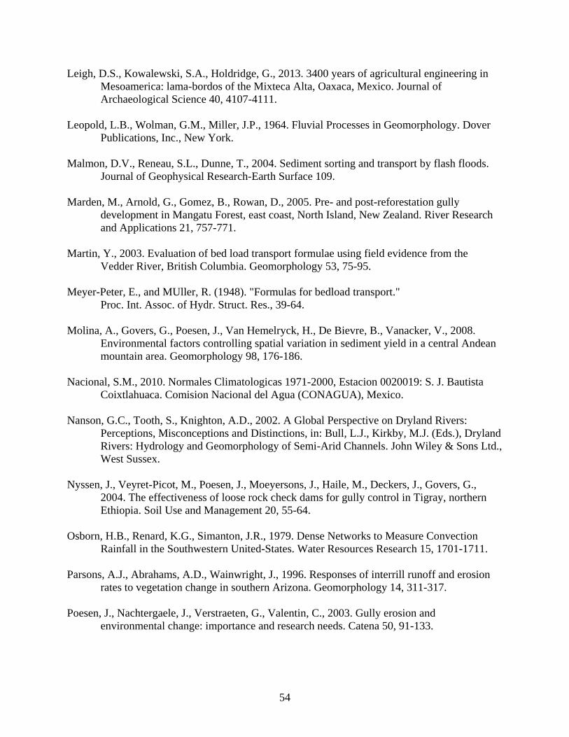
54
Leigh, D.S., Kowalewski, S.A., Holdridge, G., 2013. 3400 years of agricultural engineering in
Mesoamerica: lama-bordos of the Mixteca Alta, Oaxaca, Mexico. Journal of
Archaeological Science 40, 4107-4111.
Leopold, L.B., Wolman, G.M., Miller, J.P., 1964. Fluvial Processes in Geomorphology. Dover
Publications, Inc., New York.
Malmon, D.V., Reneau, S.L., Dunne, T., 2004. Sediment sorting and transport by flash floods.
Journal of Geophysical Research-Earth Surface 109.
Marden, M., Arnold, G., Gomez, B., Rowan, D., 2005. Pre- and post-reforestation gully
development in Mangatu Forest, east coast, North Island, New Zealand. River Research
and Applications 21, 757-771.
Martin, Y., 2003. Evaluation of bed load transport formulae using field evidence from the
Vedder River, British Columbia. Geomorphology 53, 75-95.
Meyer-Peter, E., and MUller, R. (1948). "Formulas for bedload transport."
Proc. Int. Assoc. of Hydr. Struct. Res., 39-64.
Molina, A., Govers, G., Poesen, J., Van Hemelryck, H., De Bievre, B., Vanacker, V., 2008.
Environmental factors controlling spatial variation in sediment yield in a central Andean
mountain area. Geomorphology 98, 176-186.
Nacional, S.M., 2010. Normales Climatologicas 1971-2000, Estacion 0020019: S. J. Bautista
Coixtlahuaca. Comision Nacional del Agua (CONAGUA), Mexico.
Nanson, G.C., Tooth, S., Knighton, A.D., 2002. A Global Perspective on Dryland Rivers:
Perceptions, Misconceptions and Distinctions, in: Bull, L.J., Kirkby, M.J. (Eds.), Dryland
Rivers: Hydrology and Geomorphology of Semi-Arid Channels. John Wiley & Sons Ltd.,
West Sussex.
Nyssen, J., Veyret-Picot, M., Poesen, J., Moeyersons, J., Haile, M., Deckers, J., Govers, G.,
2004. The effectiveness of loose rock check dams for gully control in Tigray, northern
Ethiopia. Soil Use and Management 20, 55-64.
Osborn, H.B., Renard, K.G., Simanton, J.R., 1979. Dense Networks to Measure Convection
Rainfall in the Southwestern United-States. Water Resources Research 15, 1701-1711.
Parsons, A.J., Abrahams, A.D., Wainwright, J., 1996. Responses of interrill runoff and erosion
rates to vegetation change in southern Arizona. Geomorphology 14, 311-317.
Poesen, J., Nachtergaele, J., Verstraeten, G., Valentin, C., 2003. Gully erosion and
environmental change: importance and research needs. Catena 50, 91-133.
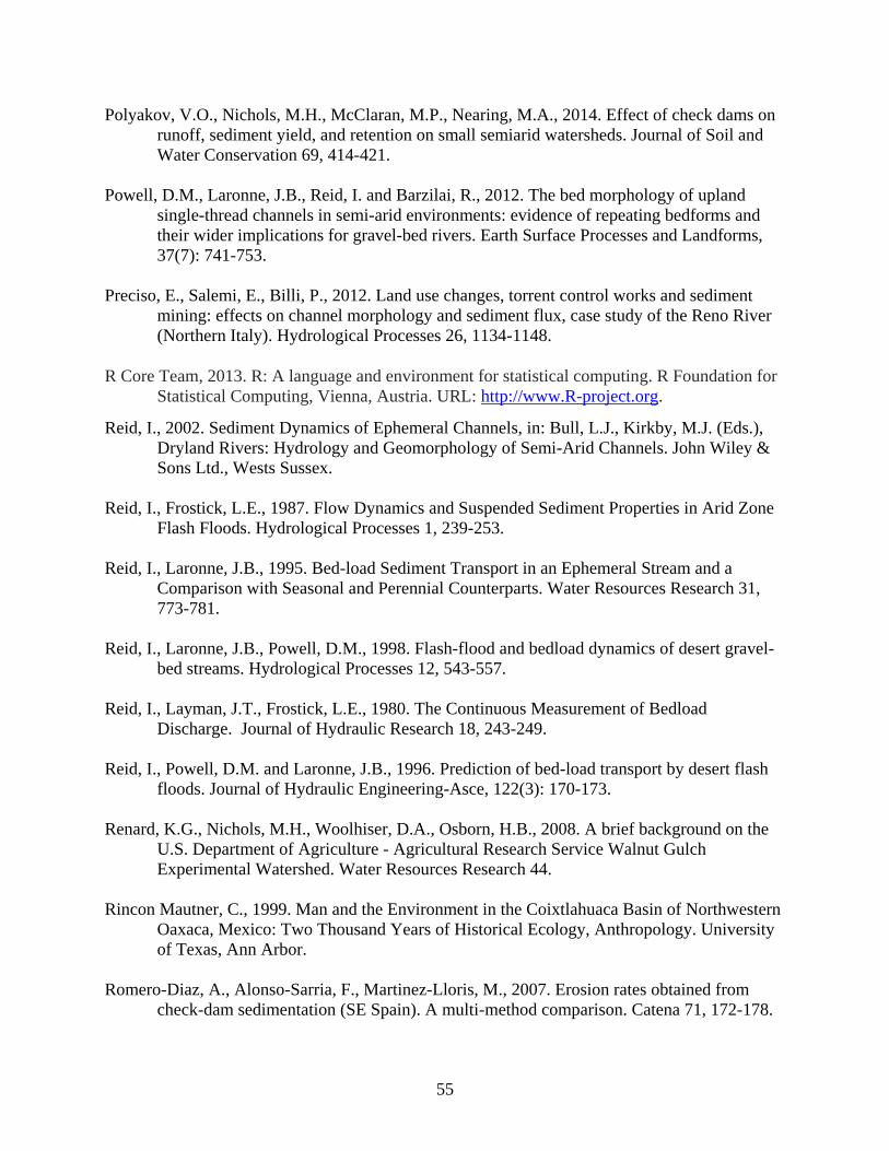
55
Polyakov, V.O., Nichols, M.H., McClaran, M.P., Nearing, M.A., 2014. Effect of check dams on
runoff, sediment yield, and retention on small semiarid watersheds. Journal of Soil and
Water Conservation 69, 414-421.
Powell, D.M., Laronne, J.B., Reid, I. and Barzilai, R., 2012. The bed morphology of upland
single-thread channels in semi-arid environments: evidence of repeating bedforms and
their wider implications for gravel-bed rivers. Earth Surface Processes and Landforms,
37(7): 741-753.
Preciso, E., Salemi, E., Billi, P., 2012. Land use changes, torrent control works and sediment
mining: effects on channel morphology and sediment flux, case study of the Reno River
(Northern Italy). Hydrological Processes 26, 1134-1148.
R Core Team, 2013. R: A language and environment for statistical computing. R Foundation for
Statistical Computing, Vienna, Austria. URL: http://www.R-project.org.
Reid, I., 2002. Sediment Dynamics of Ephemeral Channels, in: Bull, L.J., Kirkby, M.J. (Eds.),
Dryland Rivers: Hydrology and Geomorphology of Semi-Arid Channels. John Wiley &
Sons Ltd., Wests Sussex.
Reid, I., Frostick, L.E., 1987. Flow Dynamics and Suspended Sediment Properties in Arid Zone
Flash Floods. Hydrological Processes 1, 239-253.
Reid, I., Laronne, J.B., 1995. Bed-load Sediment Transport in an Ephemeral Stream and a
Comparison with Seasonal and Perennial Counterparts. Water Resources Research 31,
773-781.
Reid, I., Laronne, J.B., Powell, D.M., 1998. Flash-flood and bedload dynamics of desert gravel-
bed streams. Hydrological Processes 12, 543-557.
Reid, I., Layman, J.T., Frostick, L.E., 1980. The Continuous Measurement of Bedload
Discharge. Journal of Hydraulic Research 18, 243-249.
Reid, I., Powell, D.M. and Laronne, J.B., 1996. Prediction of bed-load transport by desert flash
floods. Journal of Hydraulic Engineering-Asce, 122(3): 170-173.
Renard, K.G., Nichols, M.H., Woolhiser, D.A., Osborn, H.B., 2008. A brief background on the
U.S. Department of Agriculture - Agricultural Research Service Walnut Gulch
Experimental Watershed. Water Resources Research 44.
Rincon Mautner, C., 1999. Man and the Environment in the Coixtlahuaca Basin of Northwestern
Oaxaca, Mexico: Two Thousand Years of Historical Ecology, Anthropology. University
of Texas, Ann Arbor.
Romero-Diaz, A., Alonso-Sarria, F., Martinez-Lloris, M., 2007. Erosion rates obtained from
check-dam sedimentation (SE Spain). A multi-method comparison. Catena 71, 172-178.

56
Romero-Diaz, A., Marin-Sanleandro, P., Ortiz-Silla, R., 2012. Loss of soil fertility estimated
from sediment trapped in check dams. South-eastern Spain. Catena 99, 42-53.
Santamaria-Diaz, A., Alaniz-Alvarez, S-A., Nieto-Samaniego, A. F., 2008. Deformaciones
cenozoicas en la Cobertura de la Falla Caltepec en la Region de Tamazulapam, sur de
Mexico. Revista Mexicana De Ciencias Geologicas 25, 494-516.
Schick, A.P., Lekach, J., Hassan, M.A., 1987. Vertical exchange of coarse bedload in desert
streams, in: Frostick, L.E., Reid, I. (Eds.), Desert Sediments: Ancient and Modern.
Blackwell Scientific Publications, Oxford.
Schumm, S.A., 2005. River Variability and Complexity. Cambridge University Press,
Cambridge.
Schumm, S.A., Hadley, R.F., 1957. Arroyos and the Semi-Arid Cycle of Erosion. American
Journal of Science 255, 161-174.
Shannon, J., Richardson, R., Thornes, J., 2002. Modelling Event-based Fluxes in Ephemeral
Streams, in: Bull, L.J., Kirkby, M.J. (Eds.), Dryland Rivers: Hydrology and
Geomorphology of Semi-Arid Channels. John Wiley & Sons Ltd., West Sussex.
Singer, M.B., Michaelides, K., 2014. How is topographic simplicity maintained in ephemeral
dryland channels? Geology 42, 1091-1094.
Tooth, S., 2000. Process, form and change in dryland rivers: a review of recent research. Earth-
Science Reviews 51, 67-107.
UN Report, 2011. Global Drylands: A UN system-wide response. United Nations Environmental
Management Group.
UNESCO, 2016. Tehuacán-Cuicatlán biosphere reserve. Ecological Sciences United Nations
Educational, Scientific and Cultural Organization,
http://www.unesco.org/new/en/natural-sciences/environment/ecological-
sciences/biosphere-reserves/latin-america-and-the-caribbean/mexico/tehuacan-cuicatlan/.
Last accessed June, 2016.
USGS, 2011. Global Land Survey , 2000, Landsat ETM+, 30m LE70250482003146EDC00,
United States Geological Survey, Sioux Falls, South Dakota.
Wakelin-King, G.A., Webb, J.A., 2007. Threshold-dominated fluvial styles in an arid-zone mud-
aggregate river: The uplands of Fowlers Creek, Australia. Geomorphology 85, 114-127.
Walling, D.E., Kleo, A.H.A., 1979. Sediment yield of rivers in areas of low precipitation: A
global view. The Hydrology of Mountainous Areas. IAHS Publ. 128, pp. 479-493.

57
Waters, M.R., Haynes, C.V., 2001. Late Quaternary arroyo formation and climate change in the
American Southwest. Geology 29, 399-402.
Zema, D.A., Bombino, G., Boix-Fayos, C., Tamburino, V., Zimbone, S.M., Fortugno, D., 2014.
Evaluation and modeling of scouring and sedimentation around check dams in a
Mediterranean torrent in Calabria, Italy. Journal of Soil and Water Conservation 69, 316-
329.
58
Figure 2.1. Map of the Rio Culebra watershed and its tributaries in Oaxaca, Mexico. Map shows the location of
some of the geomorphic attributes in the Culebra watershed and a close-up of Barranca Sauce in Santa Maria
Nativitas, and Barranca Sandage in San Juan Bautista Coixtlahuaca. (Black arrows indicate direction of flow).

59
Figure 2.2. Google Earth satellite imagery of (a) Barrancas Sauce and (b) Sandage. A close-up of the study
reaches at the basin outlets are shown below each watershed and are outlined by a dashed light blue box in the
watershed scale images. Note the bare ground (pinkish orange), endeque/calcrete (white), forest/vegetation
cover (dark green), and darker brown and terraced agricultural areas. The area with conservation works is
outlined with a solid white box.
60
Figure 2.3. Example of a modern check dam (i.e., Victor’s lama-bordos). Different views around the check
dam include: a view downstream looking upstream (a); a view of fill behind the check dam (b); a view on top
of check dam; (c) and a view of the channel bed downstream of check dam (d). Note the endeque/calcrete
(outlined in red in Figures 2.3a and d) reached deep into the valley at one point.
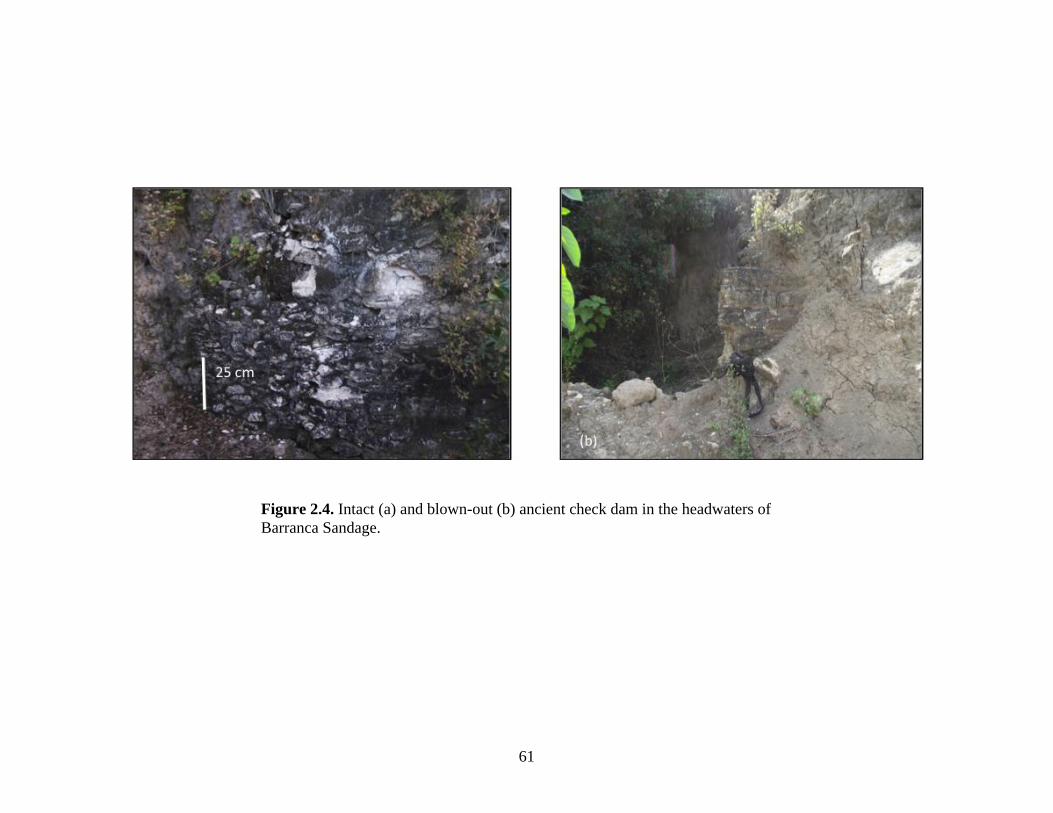
61
Figure 2.4. Intact (a) and blown-out (b) ancient check dam in the headwaters of
Barranca Sandage.
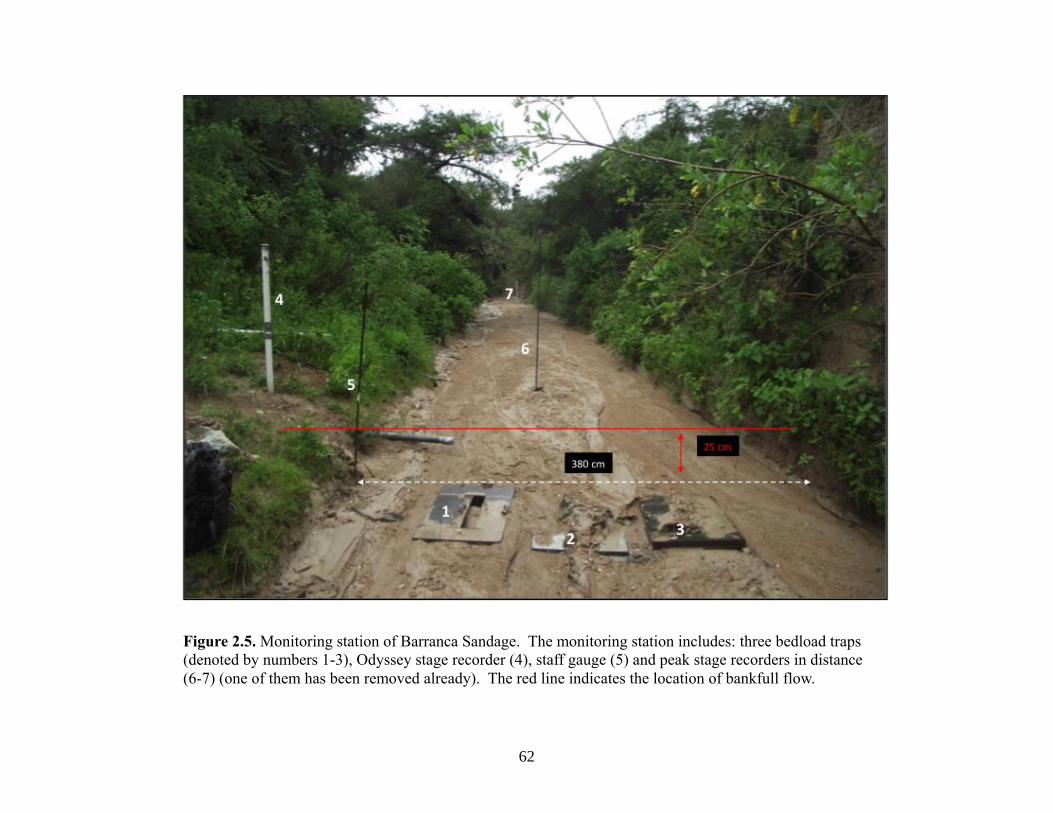
62
Figure 2.5. Monitoring station of Barranca Sandage. The monitoring station includes: three bedload traps
(denoted by numbers 1-3), Odyssey stage recorder (4), staff gauge (5) and peak stage recorders in distance
(6-7) (one of them has been removed already). The red line indicates the location of bankfull flow.

63
Figure 2.6. Monitoring station of Barranca Sauce (a). The red line indicates bankfull stage and the white dashed
line indicates channel bed width. Note that the basin outlet is much wider than in Sandage (10 m vs. 4m). Figure
(b) shows the three of the five pit traps installed in 2013, while figure (c) displays the ten pit traps after five more
were added in 2014.
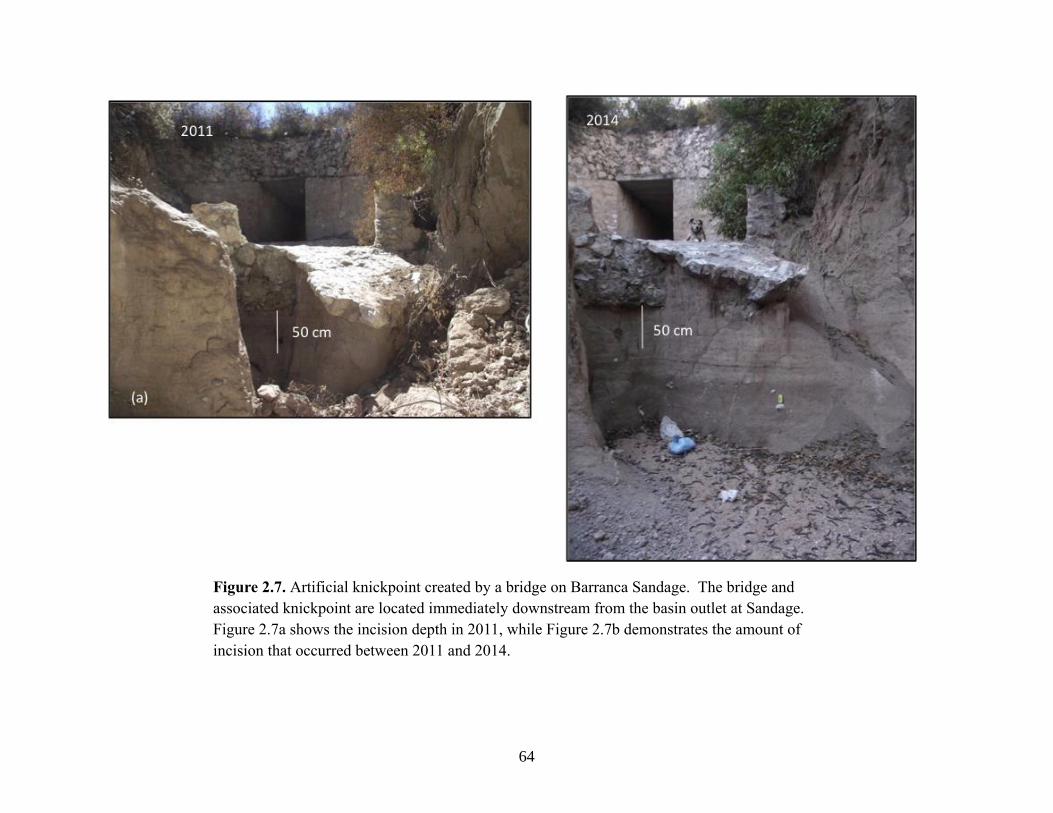
64
Figure 2.7. Artificial knickpoint created by a bridge on Barranca Sandage. The bridge and
associated knickpoint are located immediately downstream from the basin outlet at Sandage.
Figure 2.7a shows the incision depth in 2011, while Figure 2.7b demonstrates the amount of
incision that occurred between 2011 and 2014.

65
Figure 2.8. Natural knickpoints in the Río Culebra watershed. Figure 2.8a shows n exposed andesite flow
located in the upstream section of the Culebra. Figure2.8b shows a knickpoint in the Yanhuitlan beds
located in the downstream section of Barranca Sandage.
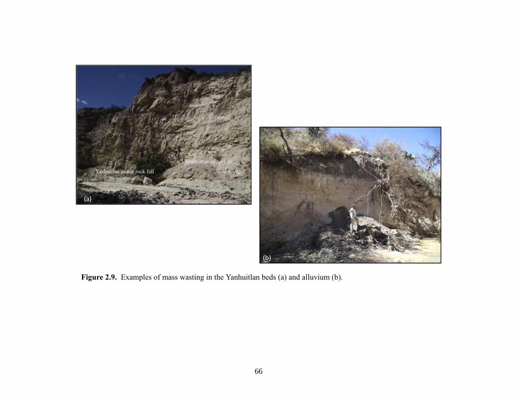
66
Figure 2.9. Examples of mass wasting in the Yanhuitlan beds (a) and alluvium (b).

67
Figure 2.10. Bed topography and morphology in Barrancas Sandage (a) and Sauce (b).
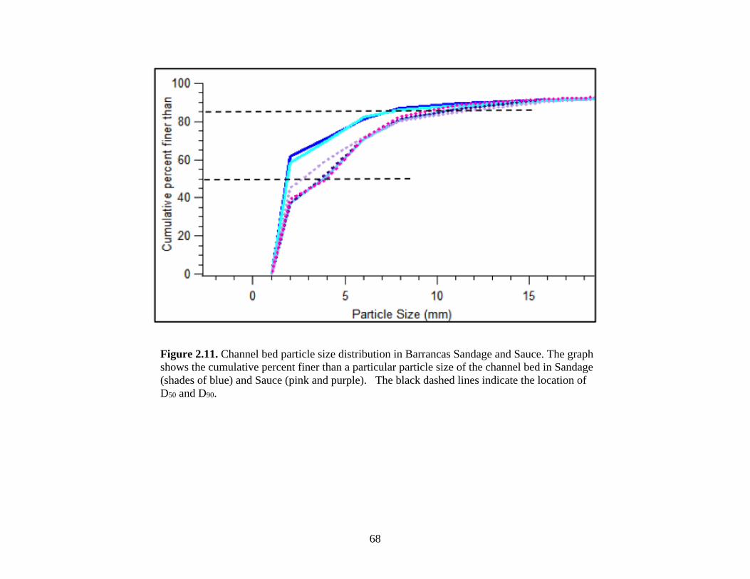
68
Figure 2.11. Channel bed particle size distribution in Barrancas Sandage and Sauce. The graph
shows the cumulative percent finer than a particular particle size of the channel bed in Sandage
(shades of blue) and Sauce (pink and purple). The black dashed lines indicate the location of
D50 and D90.

69
Yanhuitlan (Yan)
Endeque (En)
Chalcedony (CH0
Mud aggregates (M)
Seed
Volcanic (V)
Sauce
May 2013
July 2013
Feb 2014
Figure 2.12. Distribution of channel bed
material and shape in Barrancas Sandage and
Sauce. The bar graphs show particle shape
from these separate studies in Sandage (a) and
Sauce (b) between 2013-2014. The pie graphs
show the distribution of material in Sandage (c)
and Sauce (d).
Sandage
May 2013
July 2013
Feb 2014
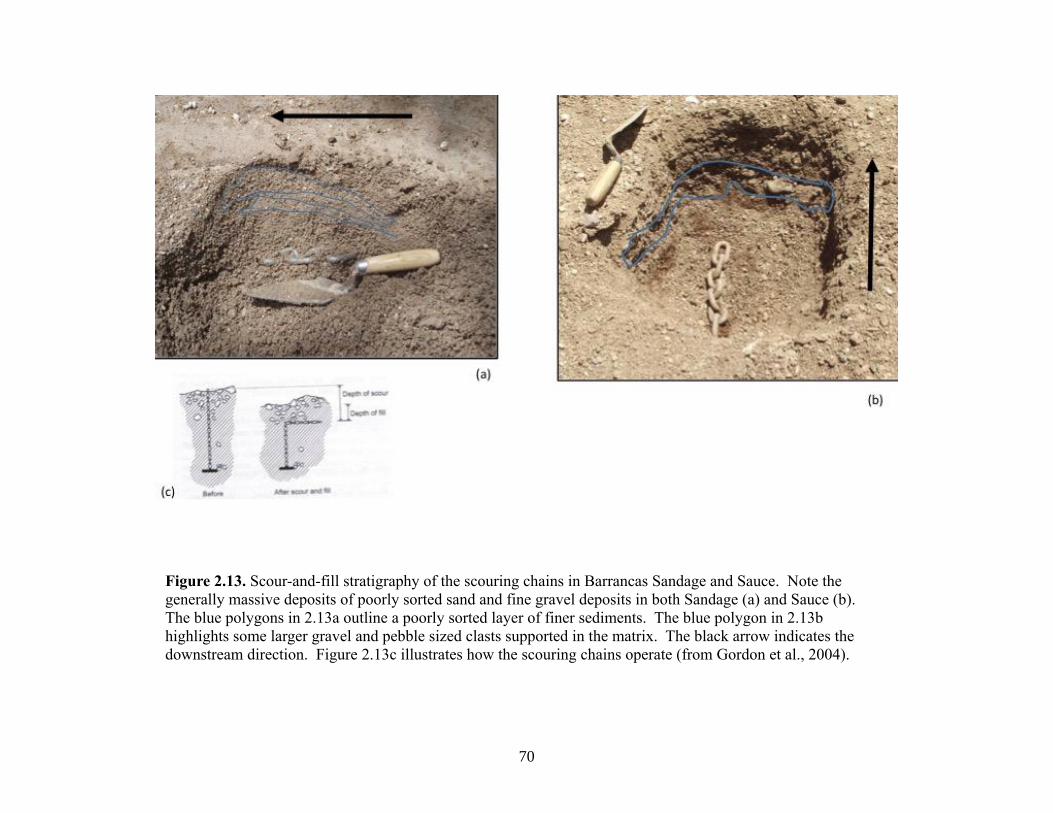
70
Figure 2.13. Scour-and-fill stratigraphy of the scouring chains in Barrancas Sandage and Sauce. Note the
generally massive deposits of poorly sorted sand and fine gravel deposits in both Sandage (a) and Sauce (b).
The blue polygons in 2.13a outline a poorly sorted layer of finer sediments. The blue polygon in 2.13b
highlights some larger gravel and pebble sized clasts supported in the matrix. The black arrow indicates the
downstream direction. Figure 2.13c illustrates how the scouring chains operate (from Gordon et al., 2004).
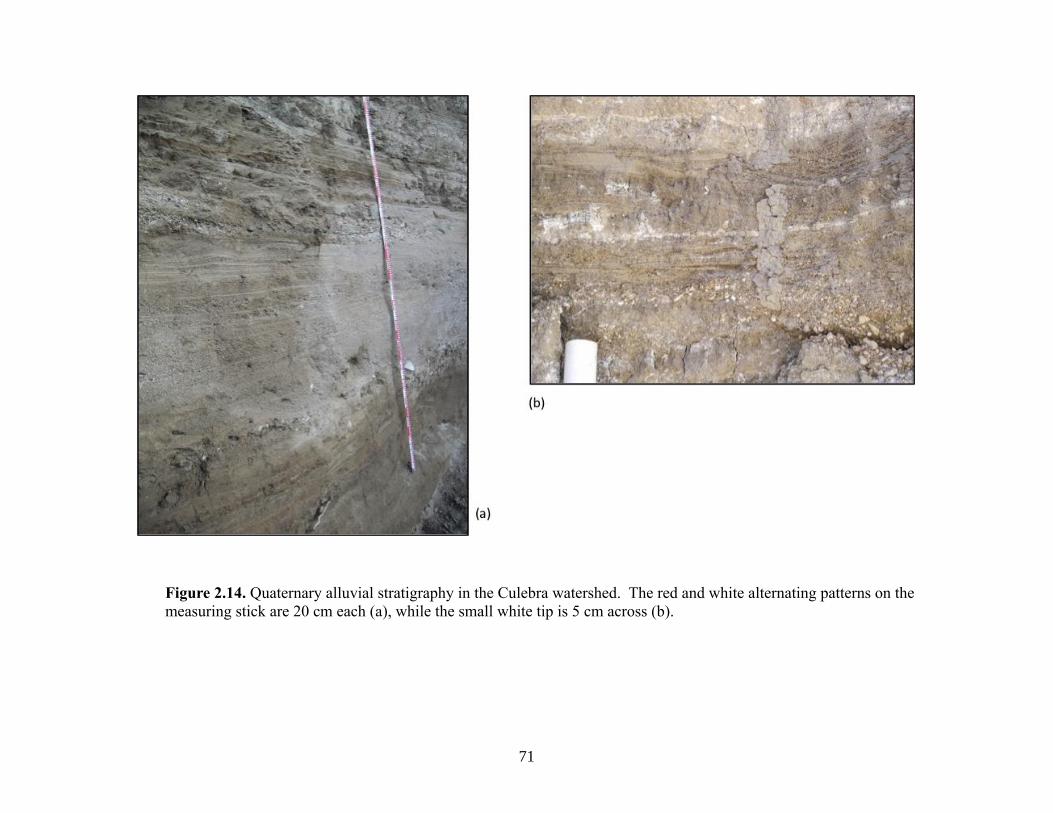
71
Figure 2.14. Quaternary alluvial stratigraphy in the Culebra watershed. The red and white alternating patterns on the
measuring stick are 20 cm each (a), while the small white tip is 5 cm across (b).

72
Figure 2.15. Particle size distribution for each floods in Sandage between 2013 (blue and purple) and 2014 (red
and green). Figure 2.15b is a focus view of the 0-10 mm particles. The dashed red line marks the D50 and D85
particle size in Figure 2.15b and a, respectively.
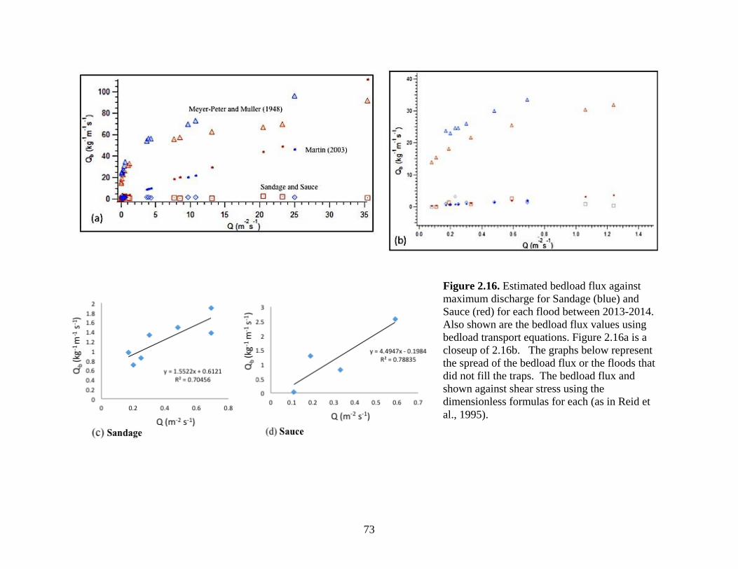
73
Figure 2.16. Estimated bedload flux against
maximum discharge for Sandage (blue) and
Sauce (red) for each flood between 2013-2014.
Also shown are the bedload flux values using
bedload transport equations. Figure 2.16a is a
closeup of 2.16b. The graphs below represent
the spread of the bedload flux or the floods that
did not fill the traps. The bedload flux and
shown against shear stress using the
dimensionless formulas for each (as in Reid et
al., 1995).

74
Figure 2.17. Estimated bedload flux values for Sandage (light blue) and Sauce (pink) against
streams from other environments (modified from Billi, 2008).
Figure 2.18. Estimated bedload yield in tonnes per day for Sandage (blue crosses) and Sauce
(red and black crosses) against streams from other environments (modified from Preciso et al.,
2012).
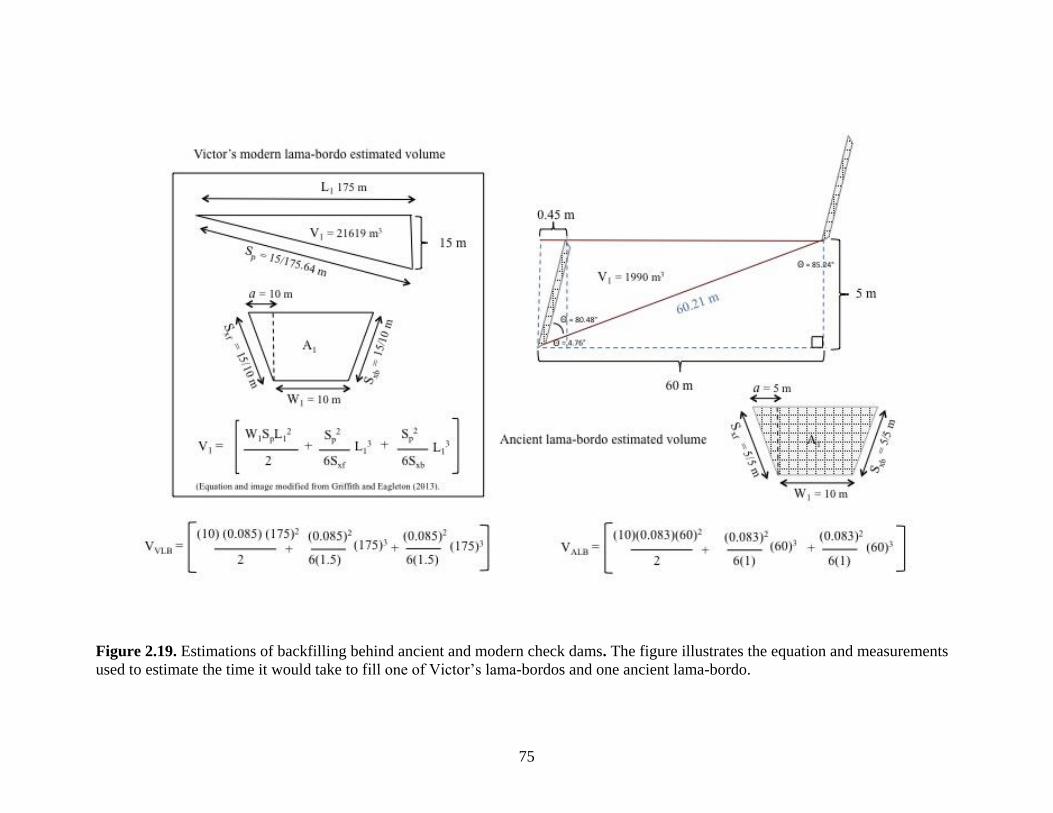
75
Figure 2.19. Estimations of backfilling behind ancient and modern check dams. The figure illustrates the equation and measurements
used to estimate the time it would take to fill one of Victor’s lama-bordos and one ancient lama-bordo.

76
Table 2.1. Land cover classification for Barrancas Sandage and Sauce.
Land Cover Class Sauce % Sandage %
Forest/vegetation 34 36
Conserved land 0 21
Calcrete 13 18
Bare Rock 28 5
Cropland 21 17
Gullying 4 3

77
(a)
(b)
Table 2.2. Scour-and-fill information for Barranca Sandage (a) and
Sauce (b) for the flood season of 2013-2014.
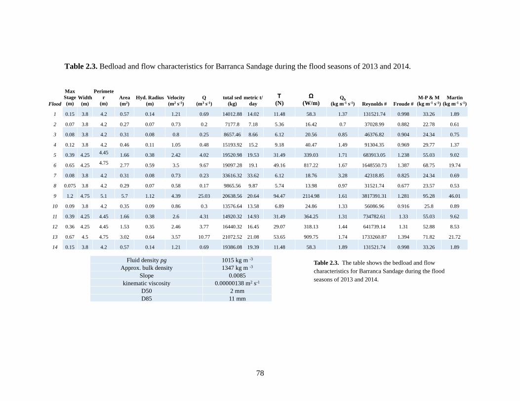
78
Flood
Max Stage
(m) Width
(m)
Perimeter
(m) Area (m2)
Hyd. Radius (m)
Velocity (m2 s-1)
Q (m3 s-1)
total sed (kg)
metric t/day
Τ (N)
Ω (W/m)
Qb
(kg m-1 s-1) Reynolds # Froude #
M-P & M (kg m-1 s-1)
Martin (kg m-1 s-1)
1 0.15 3.8 4.2 0.57 0.14 1.21 0.69 14012.88 14.02 11.48 58.3 1.37 131521.74 0.998 33.26 1.89
2 0.07 3.8 4.2 0.27 0.07 0.73 0.2 7177.8 7.18 5.36 16.42 0.7 37028.99 0.882 22.78 0.61
3 0.08 3.8 4.2 0.31 0.08 0.8 0.25 8657.46 8.66 6.12 20.56 0.85 46376.82 0.904 24.34 0.75
4 0.12 3.8 4.2 0.46 0.11 1.05 0.48 15193.92 15.2 9.18 40.47 1.49 91304.35 0.969 29.77 1.37
5 0.39 4.25 4.45
1.66 0.38 2.42 4.02 19520.98 19.53 31.49 339.03 1.71 683913.05 1.238 55.03 9.02
6 0.65 4.25 4.75
2.77 0.59 3.5 9.67 19097.28 19.1 49.16 817.22 1.67 1648550.73 1.387 68.75 19.74
7 0.08 3.8 4.2 0.31 0.08 0.73 0.23 33616.32 33.62 6.12 18.76 3.28 42318.85 0.825 24.34 0.69
8 0.075 3.8 4.2 0.29 0.07 0.58 0.17 9865.56 9.87 5.74 13.98 0.97 31521.74 0.677 23.57 0.53
9 1.2 4.75 5.1 5.7 1.12 4.39 25.03 20638.56 20.64 94.47 2114.98 1.61 3817391.31 1.281 95.28 46.01
10 0.09 3.8 4.2 0.35 0.09 0.86 0.3 13576.64 13.58 6.89 24.86 1.33 56086.96 0.916 25.8 0.89
11 0.39 4.25 4.45 1.66 0.38 2.6 4.31 14920.32 14.93 31.49 364.25 1.31 734782.61 1.33 55.03 9.62
12 0.36 4.25 4.45 1.53 0.35 2.46 3.77 16440.32 16.45 29.07 318.13 1.44 641739.14 1.31 52.88 8.53
13 0.67 4.5 4.75 3.02 0.64 3.57 10.77 21072.52 21.08 53.65 909.75 1.74 1733260.87 1.394 71.82 21.72
14 0.15 3.8 4.2 0.57 0.14 1.21 0.69 19386.08 19.39 11.48 58.3 1.89 131521.74 0.998 33.26 1.89
Fluid density pg 1015 kg m -3
Approx. bulk density 1347 kg m -3
Slope 0.0085
kinematic viscosity 0.00000138 m2 s-1
D50 2 mm
D85 11 mm
Table 2.3. The table shows the bedload and flow
characteristics for Barranca Sandage during the flood
seasons of 2013 and 2014.
Table 2.3. Bedload and flow characteristics for Barranca Sandage during the flood seasons of 2013 and 2014.

79
Table 2.4. Bedload and flow characteristics for Barranca Sauce during the flood seasons of 2013 and 2014.

80
CHAPTER 3
LATE PLEISTOCENE AND HOLOCENE ARROYO CYCLES OF THE MIXTECA ALTA,
OAXACA, MEXICO2
2 Holdridge, G., Leigh, D. S., Bernal, J.P., and Kowalewski S. To be submitted to Palaeogeography,
Palaeoclimatology, Palaeoecology.

81
Abstract
Arroyos are incised, ephemeral dryland streams that aggrade and incise on a cyclical
timescale. Arroyo studies are integral to understanding landscape evolution in drylands, but the
potential climatic drivers of arroyos are poorly understood. Additionally, human activities in the
late Holocene confound climatic influences on arroyo cycles, making it difficult to discern the
dominant drivers of erosion and sedimentation in these dryland systems. This paper presents a
study on the arroyo cycles in the semi-arid environment of the Mixteca Alta, Oaxaca, Mexico.
The characteristics and chronology of the alluvium-paleosol sequences from two watersheds in
Coixtlahuaca (this study) and one in Nochixtlan (Mueller et al., 2012) were examined and
compared to the regional δ18O signal from stalagmites from Guererro that date from the terminal
Pleistocene to the late Holocene (Bernal et al., 2011; Lachniet et al., 2013). In order to better
understand the impact of climate change before widespread agriculture began in the region, the
results corresponding to the pre-agricultural era (the terminal Pleistocene through the middle
Holocene) were compared to those from the agricultural era in the late Holocene. Overarching
regional paleoclimatic conditions partially explained periods of incision, aggradation and
paleosol formation, while studies on present-day climate and dryland stream systems offered
additional insight on various aspects of arroyo cycles. During the late Holocene, sedimentation
rates were estimated to be higher in association with widespread agricultural lama-bordos (i.e.,
check dams) than in the previous 15,000 years. The lama-bordos were very effective sediment
traps, and they supported increasing populations that took advantage of widespread aggradation.
In sum, the combination of paleoenvironmental and paleoclimatic information, archaeological
material, and modern analogues of arroyos help explain the impact of climate change and human
activities on the various geomorphic processes involved in arroyo cycles.

82
3.1 Introduction
Arroyos are flat-bottomed, incised ephemeral channels with steep walls, typically located
in arid to semi-arid environments (Bull, 1997). Studies of recent arroyo formation suggest that a
combination of external and internal factors affect cutting and filling, including: precipitation
intensity and variability, relief, lithology, soil moisture, vegetation type and cover, drainage
basin size and connectivity, duricrusts (e.g., calcrete), and human activities (e.g., deforestation,
agriculture, and overgrazing) (e.g., Graf, 2002; Poesen et al., 2003; Schumm, 2005; Valentin, et
al 2005). Although, it is recognized that arroyo cycles develop due to a multifarious
combination of internal and external factors, in most contexts, human activities and/or climatic
fluctuations exert the most influence (Harvey and Pederson, 2011). Arroyo cycles involve
incision and aggradation on a cyclical timescale, though it is unclear on what timescale and to
which climate phenomena these landforms are responding (Bull, 1991; Mann and Meltzer,
2007). Whether a stream is degrading or aggrading is in part linked to its internal thresholds
involving the balance between sediment supply versus water supply (Schumm and Hadley, 1957;
Schumm, 2005). However, it is uncertain how external human and/or climatic drivers interact
with internal thresholds to produce threshold-crossing adjustments on a regional scale (Prosser et
al., 1994; Perroy et al., 2012).
Waters and Haynes’ (2001) seminal paper (building on previous research, e.g., Bull,
1997) demonstrated that arroyos can form from climate fluctuations alone. Various climatic
factors have been suggested to cause arroyo cycles (as summarized in Hereford, 2002), including
the dry-wet-dry fluctuation model, the base level model and variants of the first model, such as
wet ‘cycles’ occurring in an overall dry period (Butzer et al., 2008). Other investigations have
invoked more process-based connections, such as the importance of rain intensity (Harvey and

83
Pederson, 2011), and the relationship between alluvial fills and flood magnitude/frequency (Ely,
1997). Various studies have proposed climatic mechanisms propelling arroyo cycles, such as
increased El Niño Southern Oscillation (ENSO) intensity (Waters and Haynes, 2001), and
fluctuations in the North American Monsoon strength (Mann and Meltzer, 2007), though these
relationships are still unresolved.
Studies of soil erosion during recent (e.g., Walling and Collins, 2008; Svoray and
Markovitch, 2009) and prehistoric (e.g., O’Hara et al., 1993; Waters and Ravesloot, 2000;
Wilkinson, 2005) times corroborate that human activities, such as agriculture and herding,
influence gullying. It is generally agreed that some combination of human and climatic factors
have resulted in widespread gully formation and erosion in drylands during the late Holocene
period (Bull, 1997; McAuliffe et al., 2001; Avni, 2005; Eriksson, et al., 2006; Borejsza and
Frederick, 2010; Constante et al., 2010). However, it is not always easy to identify which
anthropogenic factor led to landscape degradation in an area, and it is extremely difficult to
determine the degree to which climate versus human activities influence arroyo cycles.
Therefore, the history of arroyo cycles and their link to climatic stimuli must be established
before attempting to understand the connection between human activities and arroyo cycles
(Bull, 1991; Hereford, 2002; Harvey and Pederson, 2011).
Much of the difficulty in deciphering arroyo cycles is due to the relatively poor
chronological resolution of alluvial stratigraphy as well as the lack of a locally or even a
regionally continuous, high-resolution climatic record, such as one that can be obtained from
speleothems. Without external environmental proxies to provide the general climatic trend, it
leaves the interpretation of the paleohydrologic record to be derived from alluvium-paleosol
sequences that are susceptible to the problem of equifinality (Graf, 1979; Knox 1993; Nordt,

84
2004). A study by Harden et al. (2010) combined over 700 dates from deposits in the
southwestern United States into cumulative probability density function plots and compared
them to the δ18O record from a stalagmite from Pink Panther Cave in Arizona studied by
Asmerom et al. (2007). This comparison of dated slackwater and other alluvial arroyo deposits
against the stalagmite proxy data has increased our understanding of the relationship between
past hydrology and climate. However, despite this and other studies on arroyo cut-and-fill
stratigraphy, many questions still remain about the precise nature of overarching climatic
phenomena that cause regional scale incision and aggradation, and the relative contributions of
anthropogenic and climatic drivers in the late Holocene. Furthermore, there are inconsistencies
in the approach to studying arroyos. For example, many studies in the southwestern U.S.
emphasize dating arroyo incisions and the sediment fills of the arroyos, while in Mexico many
studies focus on paleosols. Finally, there is a need for more rigorous qualitative analyses
between climatic fluctuations and alluvial histories.
This paper presents alluvium-paleosol sequences from the Río Culebra in the San Juan
Bautista Coixtlahuaca and Santa María Nativitas municipalities, and the Río Inguiro in the Santa
Magdalena Jicotlan municipality, both of which are located in the Mixteca Alta, Oaxaca,
Mexico. The Mixteca Alta is known for its highly degraded landscape and deep arroyos, locally
known as barrancas (Mueller et al., 2012; Leigh et al., 2013). Since the Formative period (local
Cruz phase 3,500-2,250 cal BP), prehistoric agriculturalists built check-dams (known as lama-
bordos) and terraces to mitigate soil erosion (Kowalewski et al., 2009), and the earliest known
lama-bordos were documented in Barranca Sandage in Coixtlahuaca circa 3,500 cal BP (Leigh et
al., 2013). Evidence of widespread lama-bordo and terrace constructions is observed by the
Post-Classic period (i.e., local Natividad phase, 1,250-430 cal BP) (Kowalewski et al., 2009).

85
These constructions persist today in various parts of the landscape. The geology,
geomorphology and widespread barranca development is similar to the nearby headwaters of the
Río Verde watershed in the municipality of Santa María Nochixtlan (Mueller et al., 2012), the
results of which are incorporated in the discussion of this paper.
3.1.1 Objectives
The main objectives are twofold: 1) to better understand the relationship between climate
and widespread arroyo development during the pre-agricultural era, and 2) to use this climate-
arroyo relationship to better discern the impact that humans had during the agricultural era. The
results from the Ríos Culebra and Inguiro (this study) were combined with the results from the
Río Verde (Mueller et al., 2012) and compared to the stable oxygen isotopic proxy data obtained
from stalagmites from various caves in Guerrero (Bernal et al., 2011; Lachniet et al., 2013) to
better understand the relationship between the paleoclimate and paleohydrology. For the late
Holocene, the grain size data from El Junco Crater Lake (Conroy et al., 2008) was also examined
as a proxy for ENSO intensity against the paleosol and alluvium ages. A basin-wide approach,
as utilized in this study, can help discern between local developments and intrinsic or complex
response and basin-wide response to climatic drivers (e.g., Holliday, 1985).
3.2 Study Area
Stratigraphic investigations were conducted in the arroyos of Coixtlahuaca, Nativitas, and
Jicotlan municipalities (Figure 3.1; see Appendix II for coordinates). Profiles in the
municipalities of Nativitas and Coixtlahuaca are situated within the Río Culebra watershed (or
Culebra watershed), while Jicotlan is located along the Río Inguiro watershed. The profiles in
Nochixtlan studied by Mueller et al. (2012) are located in the Río Verde watershed (Figure 3.1).

86
All of these study sites are located in the Mixteca Alta, Oaxaca, Mexico, which is
situated, on average, 2,300 m above mean sea level (amsl). The Mixteca Alta is a part of the
Mixteca macroregion, which designates the present area of the Mixtec culture and language
groups. The Alta (‘high”) of Mixteca Alta represents the high altitude, inland semi-arid region,
which is distinguished from the Baja (‘low”) and Costa (“coastal”) sub-regions (Balkansky et al.,
2000). The Ríos Culebra and Inguiro are situated in the headwaters of the Río Papaloapan,
draining the eastern part of the continental divide, created by the Sierra Madre del Sur, towards
the Gulf of Mexico. Conversely, the Río Verde watershed drains the western part of this
continental divide, towards the Pacific Ocean. Mueller et al., (2012) studied several headwater
tributaries to the Río Verde, but their study will be referred to as the Río Verde watershed.
The regional climate is characterized as semi-arid (BSh Köppen classification), with an
average temperature of between 13.2-18.6 ºC and receiving an average of approximately 528 mm
of rain per year (Servicio Meteorologico Nacional, 2010). The warmest time of the year, May
through October, overlaps with the rainy season, which peaks in June and again in September.
The high terrain of the Sierra Madre del Sur, in which the Mixteca macroregion is situated,
causes a rain shadow in the region, and the North American Monsoon (NAM) is the main source
of precipitation. The timing and duration of NAM are predominantly controlled by the
movement of the Intertropical Convergence Zone (ITCZ) and the intensity of El Niño Southern
Oscillation (ENSO) (Trejo, 2004; Vera et al., 2006). Although no local high-resolution climatic
proxies exist for the Mixteca Alta, stalagmite data from Guererro, located 191 kilometers away
on a heading of 257° in the Sierra Madre del Sur have been used to estimate high-resolution
regional signals of past climate (Bernal et al., 2011; Lachniet et al., 2013). The stalagmite record
consists of five different stalagmites from two caves: Juxtlahuaca cave (17°26’ N, 99°15’ W) and
87
Cueva del Diablo (18°11’ N, 99° 55 W) (Figure 3.1). A strong negative significant correlation (-
0.62, with a 5-yr smooth with 0-yr lag) was found between the oxygen isotopes from the
Guerreran and rainfall in Oaxaca for the last 128 years (Lachniet and Bernal, accepted in press).
These results suggest that the stalagmites from Guerrero can be used as a corollary to the
climatic conditions in southwestern Oaxaca from the late Pleistocene to the present (Lachniet
and Bernal, accepted in press). The δ18O isotopic signature from stalagmites is a reflection of the
regional climatic processes, which reflects precipitation in the tropics (McDermott, 2004;
Fairchild et al., 2006; Lachniet, 2009). Support for regional response to climate also comes
from a study on tree growth in Mexico, which indicated that tree growth in southwestern Mexico
(as opposed to northwestern and northeastern Mexico) was most sensitive to spring rainfall
(April-June), corresponding to the onset of the North American Monsoon (Therrell et al., 2002).
The geology of the study area primarily consists of lower to middle Tertiary siltstones
and claystones (shales), referred to as the Yanhuitlan Formation, which is overlain in areas by
middle Tertiary volcaniclastics (Teotongo volcaniclastics) and andesites (Cañada Maria andesite
and Yucudaac andesite) (Santamaria-Diaz, 2008). Calcrete surfaces (locally referred to as
“endeque”) are exposed on most hillslopes and barranca development is widespread (Kirkby,
1972; Rincon, 1999; Leigh et al., 2013).
Earthquakes do occur in the Coixtlahuaca District, but no recent major earthquakes or
faulting have been documented (Servicio Sismologico Naciónal, 2014). No faults were observed
in the Quaternary strata within the survey area based on an extensive pedestrian survey of more
than 100 km2. Since the Tertiary shales are jointed and easily erodible and no recent faults have
been observed, it was concluded that the deep incision that characterizes this valley is directly
88
related to past (and present) climate fluctuations and human activities, rather than tectonic
activity or base level change.
The valley fill comprises Quaternary alluvium situated along the mainstem of Río
Culebra and its tributaries. The Río Culebra and its tributaries are single-thread dryland streams
that have incised from about seven to thirty-seven meters below the ground surface (e.g. the
Colonial terrace). The headwaters of the Río Culebra entail an incised spring-fed stream flowing
from two sources located along the hillslope of the nearby extinct volcano, Monte Verde,
Nativitas.
3.2.1 Archaeology
Archaeological surveys of the Ríos Culebra and Inguiro, and the surrounding areas have
shown that the region exhibits a rich material record of cultural changes (Figure 3.2, Table 3.1),
especially in the last 3,500 years (Balkansky et al., 2000; Kowalewski et al., 2009). Surveys in
2008 and 2011 indicate that Archaic artifacts exist in the region, but are poorly understood. The
Formative period (local Cruz phase) is scattered throughout the Culebra and Inguiro watersheds,
but is best preserved along a tributary to the Culebra, Barranca Sandage. The Formative period
corresponds to the transition from hunting and gathering to an agricultural way of life
(Kowalewski et al., 2009). Since the early Cruz phase, prehistoric agriculturalists built check-
dams (locally referred to as lama-bordos) and terraces to mitigate soil erosion (Kowalewski et
al., 2009). The earliest known lama-bordos were documented in Barranca Sandage and dated to
~3,500 cal BP (Leigh et al., 2013).
Between 2,250 cal BP to 1,750 cal BP, population remained fairly low during the Ramos
phase, but town centers moved to the protected hillslopes. Some agricultural lama-bordos span
the entire valley floor. During the early Transición/las Flores phase (1,750-1,250 BP),
89
population first increased significantly in the Culebra and adjacent watersheds, and then was
followed by a sharp population decline and settlement dispersal. Subsequently, during the local
Natividad phase (1,250-430 cal BP), population exploded, and one of the major Post-Classic
urban centers of the Mixteca emerged in Inguiteria, Coixtlahuaca. Terrace walls are located
throughout the valley during this period (Rincon, 1999; Kowalewski et al., 2009).
The Río Verde watershed shares a similar cultural history, including the practice of
building lama-bordos and terrace walls that were dated to as early as ~2,990 cal BP (Mueller et
al., 2012).
3.3 Methods
After a thorough reconnaissance in the Culebra and Inguiro watersheds, ten profiles were
selected for more in-depth descriptions and sampling (Figure 3.3; see Figure 3.1 for location; see
APPENDIX II). Arroyo cut-and-fill features and well-represented alluvium-paleosol sequences
were selected for examination. The steep, tall, unstable, and erodible nature of arroyo walls
made accessing certain strata very dangerous. Thus, most profiles were not recorded in one
continuous section. Instead, profiles were described and sampled in several more accessible
subsections that combined to represent a continuous section. All of the stratigraphic profiles
have been described according to the nomenclature of the USDA Soil Survey (Soil Survey Staff,
1993). For each recorded profile, approximately 50 grams of sediment were obtained by
sampling at arbitrary intervals of 30 cm or according to horizon boundaries when they were
abrupt. Paleosols were identified and distinguished from unweathered alluvium by a
combination of two or more of the following factors: (1) darker color; (2) clear expression of
pedogenic structure; (3) evidence for translocation of clay; and (4) evidence for pedogenic
90
translocation of other minerals (e.g., CaCO3 or Fe2O3) (Birkeland, 1984; Schaetzl and Anderson,
2005). It is acknowledged that paleosols form in alluvium and that alluvium serves as the parent
material for paleosols. Accordingly, the term “alluvium” will be used to designate the
unweathered or apedal sediment that separates paleosols.
3.3.1 Soil Residence Time and Radiocarbon Dates
Multiple samples containing charcoal flecks and organic-rich buried A horizons were
taken for 14C dating (Table 3.2). Radiocarbon accelerator mass spectrometry (AMS) analyses
were done at the Center for Applied Isotope Studies (CAIS) at the University of Georgia using
standard pretreatment techniques. The software program CALIB (Stuiver et al., 2015) was used
to calibrate all of the ages based on the INTCAL13 database (Reimer et al., 2013). All ages are
presented as the median age in calibrated years before present (cal BP) unless otherwise noted
(Table 3.2). All age ranges are equivalent to the two-sigma range calculated by the CALIB
software from the original radiocarbon age.
Charcoal samples comprised 23 of 25 alluvium ages and ten of the 22 paleosol ages. The
remaining ages came from bulk organic material from buried A horizons and in two instances
redeposited organic material was dated to represent alluvium deposits. A total of 31 radiocarbon
dates from the Río Verde (Mueller et al., 2012) were incorporated into this study, all of which
were from organic-rich buried A horizons.
Problems with both charcoal and bulk organic dates are recognized. For example, both
can be eroded and redeposited into much younger alluvium and yield dates much older than the
actual time of alluvial deposition. Bulk organic ages can also be affected by soil residence time
(SRT) and appear older (Rincon, 1999; Leigh et al., 2013) than the time of burial of the soil
surface. Observing the dates against depth for each profile (Figure 3.3), there are a few
91
instances of inverse stratigraphy illustrating the incorporation of older organic material into
younger A horizons, and these inverted ages were not considered further (Figure 3.3, Table 3.2).
Age-depth models were constructed with the program R (version 0.98.1103) using the package
for ‘classical’ age-modelling (CLAM) of radiocarbon sequences (Blaauw, 2010; version 2.2),
which helped to assess the accuracy of bulk ages versus charcoal ages. It was found that in most
cases both were accurate, but the charcoal ages appear more consistent.
In order to consider the SRT for the bulk organic ages, the difference between calibrated
charcoal and bulk ages obtained from the organic matter of buried A horizons at five different
profiles was examined. The charcoal ages were, on average, 273 years younger than the bulk
organic ages with a standard deviation of 22 years. Since there is inherent variability in the
calibrated radiocarbon ages, a t-test was conducted to determine if the average variability in the
original calibrated date range of the charcoal and organic bulk ages was significantly different
from the average difference between the calibrated charcoal and organic bulk ages from the same
strata. No significant difference was observed between the 2-sigma error of the original
calibrated age range and the average difference between the calibrated charcoal and organic bulk
ages from the same strata (see Appendix III). Since only the calibrated age range was
incorporated into the qualitative analyses, the 2-sigma error of the original calibrated ages were
considered to represent a sufficient amount of variability to compensate for the SRT of an
organic age.
3.3.2 Geochemical Analyses, Particle Size Determination and Sedimentation Rates
Geochemical studies involved total elemental analysis on later strata using the four-acid
“near-total” procedure (ALS Geochemistry, ME-ICP61). The results of 23 elements were
provided in percentages or parts per million. Two of the elements were used to examine
92
weathering (as described in Buggle et al., 2011). Organic and inorganic content was estimated
using the loss-on-ignition procedure applied to subsamples of strata from several profiles. To
estimate the percentage of organic carbon, subsamples of each stratum were oven-dried at
105°C, weighed and then heated in a muffle furnace at 550°C for four hours (as recommended in
Heiri et al., 2001). After, the samples were cooled, weighed, and then reheated to 950°C for two
hours to burn off the inorganic carbon (as in Heiri et al., 2001).
All of the sampled strata were air-dried and sieved for particle size determination using
the <2mm U.S. sieve size to seperate <2 mm from >2 mm. The < and >2 mm fraction was
weighed and converted to percent based on the total weight. Sedimentation rates were modeled
using the CLAM program (Blaauw, 2010) in R software (R software team, 2008). The CLAM
program models the sedimentation rate based on the relationship between age and depth of each
profile’s stratigraphy.
3.3.3 Qualitative Analyses
The calibrated age range of the dated samples from the Ríos Culebra, Inguiro and Verde
watersheds were combined to generate summed probability curves. Two different summed
probability curves were created using the two-sigma calibrated age range: one for paleosols, and
one for alluvium (see APPENDIX III). In order to discern the relationship between past climatic
drivers and paleoenvironmental change, the summed probability curves and the δ18O isotope
values from the Guerreran stalagmites were examined qualitatively from the late Pleistocene to
the middle Holocene.
Difficulties in distinguishing wet versus dry in the δ18O isotope record during the late
Holocene resulted in exploring alternative paleoclimatic proxies for ENSO. Bernal et al. (2011)
demonstrated that ENSO was the dominant climatic driver during the late Holocene, following

93
the shift of the ITCZ towards the south (Haug et al., 2001). The grain size data, in particular the
sand percentage data from the El Junco Crater Lake in the Galápagos Islands is a proxy for
ENSO frequency and intensity in the eastern tropical Pacific (Conroy et al., 2008). Conroy et al.
(2008) found that the amount of sand (%) increased during increased El Niño activity (the
negative anomaly of ENSO), which in El Junco corresponds to an increase in the number of
intense rainfall events. The sand percentage data were examined against the δ18O isotope record
and the summed probability plots for the late Holocene to discern any relationships between
them. The ENSO variability determined from the El Junco record is considered only as an
approximation of regional patterns in the eastern Pacific, and it is realized that local conditions in
southwestern Mexico may differ to an extent.
3.4 Results
The alluvium-paleosol stratigraphy of ten profiles along the Ríos Culebra and Inguiro
were examined in detail (Figure 3.3; see Appendix II for profile descriptions). Two profiles
were selected along the middle section of the Río Culebra (profiles C2 and C3), while profile C1
was located in the headwaters of the Río Culebra along the second-order tributary of Barranca
Sauce. Four profiles were selected for study along the upper, middle, and lower sections of the
tributary Barranca Sandage (profile S4, S5, S6 and S7), and one profile was examined along a
first-order tributary to Barranca Sandage (profile S8). Another profile was recorded along the
lower section of the tributary Barranca Sandaxne (X9). Finally, one profile was studied along
the mid-section of the Inguiro mainstem (I10). The majority of the profiles were studied along
Barranca Sandage as it contained the most continuous and well-preserved archaeological
evidence. Some of the profiles studied along this barranca were located adjacent to lama-bordos.
94
3.4.1 Profiles on the Río Culebra
Profiles C1, C2 and C3 reflect much of the long-term depositional and erosional history
of this watershed. The headwater location, profile C1, contains well-preserved cut-and-fill
stratigraphy, with four clearly recognizable cuts (in addition to the present-day incision) and four
fills. Three paleosols bury all of the cut-and-fill stratigraphy, while one early paleosol is situated
at the bottom of the profile, into which all of the later arroyos incised.
Profile C2 is located along the midstream of the Río Culebra (Figure 3.4) and contains
much information concerning the depositional and landscape history of the basin. Its deposits
span the late Holocene to the late Pleistocene (and possibly earlier). Ten paleosols formed in
these deposits, providing information about the long-term changes in paleohydrology and
stability of the basin. A sequence of tuff deposits overlying a debris flow deposit sets this profile
apart from the others, and indicates a time of volcanism and instability in the region sometime
during the late Pleistocene.
Profile C3 is located at the confluence of Barranca Sandaxne and Río Culebra. This
profile reveals much about the end of the late Holocene with eight meters of fill corresponding to
the last 1,200 years. Three weak paleosols with A-C and A-Bw-C sequences formed within
these eight meters of late Holocene deposits, alternating with alluvium deposits. Below the eight
meters of deposits, about 24 m of stratigraphy was either covered by recent colluvium or was too
steep to sample.
3.4.2 Barrancas Sandaxne and Sandage
Two profiles located along the lower sections of Barrancas Sandaxne (X9) and Barranca
Sandage (S4) contain evidence for a long alluvial history spanning the late Pleistocene through
the late Holocene, though possibly not as continuous as in the Río Culebra. The X9 profile is
95
located along the downstream part of Barranca Sandaxne after it joins with Barranca Sandage.
Profile X9 accounts for approximately 15,000 years of stratigraphy, based on a date from the
bottom of this profile, which is around 23 m below the ground surface. Colluvium covered the
strata between 9.30 m and 15.50 m below the ground surface, impeding examination. The
studied portion of Profile X9 consists of many alluvial deposits interstratified with four major
paleosols. The paleosols span the terminal Pleistocene to the middle Holocene, and include two
Ab-Bt soil horizon sequences, and two Ab-Bw soil horizon sequences.
S4 is another profile with a long depositional history, which is located on the downstream
part of Barranca Sandage, just before it links up with Barranca Sandaxne. The upper seven
meters of S4 correspond to the middle and late Holocene, while the bottom six meters span from
the early Holocene into the late Pleistocene. This profile contains five paleosols, three of which
belong to the terminal Pleistocene-early Holocene transition. The two other paleosols consist of
thick cumulic buried A horizons dating to the middle and late Holocene.
The remaining four profiles (S5, S6, S7, and S8) studied along Barranca Sandage contain
late Holocene strata, including profiles that are directly associated with lama-bordos. The
archaeology associated with the stratigraphy will be addressed in the discussion section (5.1). S5
is in the mid-section of Barranca Sandage and is associated with a well-preserved lama-bordo,
behind which 12 m of Holocene alluvium were trapped (Figure 3.5). Profiles S6 and S7 are also
located along the mid-section of Barranca Sandage, but closer to the headwaters than S5. S6 is
situated about 20 m upstream from a lama-bordo and has five paleosols, three of which are
within the upper three meters of strata and belong to the late Holocene. The only profile studied
along a first-order tributary was S8, situated along the hillslopes of Barranca Sandage. S8 has

96
two important paleosols, which entail an Ab-C sequence and an Ab-AB-Bk separated by a thin
layer of alluvium.
3.4.3 Río Inguiro
Only one profile, I10, was studied along Río Inguiro in Jicotlan. Profile I10 is located in
the upper section of this river, just below the headwaters. The most interesting aspect of this
profile, which is set along a meander bend, is the remnants of several lama-bordos. The profile
contains five paleosols, with intermittent sediments all dating to the late Holocene. A small
stone feature, possibly a wall, is situated above the lowest sediments dating to approximately
4,100 cal BP.
3.4.4 Alluvium-Paleosol Stratigraphy
The profiles present information on the environmental history of the Culebra and Inguiro
watersheds since the late Pleistocene to the present. The stratigraphy will be presented according
to the following time periods: late Pleistocene (~27,000 to 14,700 cal BP); terminal Pleistocene
(14,700 to 11,700 cal BP); early Holocene (11,700 to 8,200 cal BP); middle Holocene (8,200 to
4,300 cal BP); and late Holocene (4,300 cal BP to the present).
3.4.4.1 Late Pleistocene (~27,000-14,700 cal BP)
Only three strata were dated to this period, two of which were paleosols having an age
between 30,000 and 27,000 cal BP, while the other stratum comprised a layer of alluvium dating
to 15,203 cal BP. Thick (> 2m), dark, cumulic buried A horizons having slickensides were
observed in the deepest portions of the stratigraphic profiles at various places in the Culebra and
Inguiro watersheds. The upper 5-10 cm of one of these thick buried A horizons was dated along
Barranca Sandage, which returned an age of 27,677 cal BP. The other Ab horizon, also located
on Barranca Sandage, was dated indirectly by radiocarbon dating of an in-situ horse jaw with

97
seven teeth (identified by Eduardo Jimenez-Hidalgo), resulting in an age of 29,716 cal BP. No
strata have been dated in the Verde watershed corresponding to the late Pleistocene, though early
strata are mentioned in the text (Mueller et al. 2012).
A layer of charcoal within a silty matrix, 23 m below ground surface at site X9, had an
age of 15,203 cal BP. Part of the cut-and-fill stratigraphy is observed in the lower strata, which
contains planar beds at the bottom. Above these beds was a fining upward sequence of large
gravel to sand with trough cross-bedding that was covered by a layer with flame structures.
3.4.4.2 Terminal Pleistocene (from 14,700-11,700 cal BP)
Paleosols dating between 13,000 and 12,000 cal BP are situated at the C2 and the X9
profiles. At profile X9, a buried A horizon with abundant charcoal was dated to 12,583 cal BP.
This weak paleosol (Ab-Bw-C sequence) was covered by nine meters of alluvium including
trough cross-bed stratigraphy, and silty and clay rhythmites. At the top of the thick alluvium was
another weak paleosol (Ab-Bw-C sequence), which was capped with by another layer of
alluvium with an age of 10,474 cal BP. At profile S4 an alluvial deposit had an age of 11,119 cal
BP. At profile C1, an age of 12,520 cal BP corresponded to the middle layers of one of the fills
containing charcoal. The bottom of the cut-and-fill at profile C1 was fairly rapid as evidenced
by rip-up clasts of this buried A. At profile C2 an Ab horizon (12,717 cal BP) with moderate
subangular blocky structure, silty loam texture, and a few calcium carbonate (CaCO3) nodules
had formed over silt deposits (A-C sequence). Overlying this Ab, a well-developed paleosol
with an A-AB-Btk-Ck sequence developed below alluvium deposited at approximately 9,063 cal
BP. This buried A-AB has a cumulic component, and the Btk has CaCO3 nodules, clay films,
prismatic structure, and slickensides in its lowermost part.

98
Some stratigraphy was situated below strata dating to the terminal Pleistocene, making it
unclear to which period they belong (e.g., terminal or late Pleistocene). For example, paleosols
below strata dating to 12,533, 11,119 and 12,717 cal BP were located at profiles C1, S4, and C2,
respectively. Some of these paleosols have a darker color (10YR 4/2) medium to strong
prismatic structure, and common, prominent slickensides in the buried A horizon (e.g., indicating
polygenesis); whereas other Abs have a browner color (10YR 5/3) and medium to strong
subangular blocky structure. Most of the soils have a B horizon, varying between a Bt, Bk, Btk
or Bw.
At profile C2, a colluvial layer beneath a terminal Pleistocene paleosol dated at 12,717
cal BP buries a tuff deposit consisting of a massive deposit of medium sand-sized particles.
Situated below the tuff is a debris flow with gravel, cobbles, and boulders in a sandy loam
matrix. Tuff has been identified in other areas of the Culebra, especially along its mid-section
(pers. Obs.; Rincon, 1999) suggesting at one point there must have been an eruption nearby;
though at a later date than the andesite flows dating to the middle Tertiary (see Santamaria-Diaz
et al., 2008). The paleosol below the debris flow is characterized by an Ab-Bk sequence with
manganese nodules, which is about a meter and a half below the bottom of the tuff. Underneath
about two meters of unaltered alluvium lies a Bw-BC, the overlying Ab having been eroded.
Another paleosol sequence is situated about a meter below the former, having an Ab-Btk with
few, distinct clay films, and few, very coarse, irregular-to-spherical CaCO3 nodules between
peds.
3.4.4.3 Early Holocene (11,700-8,200 cal BP)
Few strata have been directly dated to the early Holocene, but some strata fall between
those dating to the middle Holocene and terminal Pleistocene and are possibly early Holocene

99
layers. An age of 9,063 cal BP dates a Ck horizon at profile C2, and the overlying solum
apparently has been eroded away. Preserved above and below this Ck are about 70 cm of
alluvial deposits. At profile X9, a thin Ab paleosol sequence is formed above sediments dating
to 10,474 cal BP. A-Bw-BC sequence overlies the former paleosol, and the BC had an age of
9,625 cal BP.
3.4.4.4 Middle Holocene (8,200-4,400 cal BP)
Similar to the early Holocene, few paleosols and alluvium have been dated to the middle
Holocene. Above the Ab-Bw-BC sequence (mentioned above) at profile X9 lies an A-Bw-C
sequence, which had a cumulic Ab with an age of 6,375 cal BP. Profile S4 contains an A-C
paleosol sequence with a prominent cumulic Ab with some evidence for colluvial input. The
upper and lower part of the cumulic Ab horizon returned two different ages: 6,282-and 6,620 cal
BP, respectively. The only middle Holocene date obtained for alluvium comes from a bulk date
on an organic deposit at the bottom of a cut nearby site S5, which cuts into the paleosol dated to
the late Pleistocene, approximately 27,677 cal BP. The organic deposit has an age of 6,527 cal
BP.
3.4.4.5 Late Holocene (4,300 cal BP to the present)
Many paleosols and alluvium are dated to the late Holocene, due to better preservation of
younger sediments, as well as slightly biased sampling to obtain geomorphological data relating
to the archaeological findings. At approximately ~4,300 cal BP, paleosols were found in several
areas in the Culebra watershed. For example, at profile S4, an age of 4,360 cal BP corresponds
to a thin A/C horizon, while at profile S6, a buried A of an A-C sequence returned an age of
4,348 cal BP. At profile S8, a well-developed soil sequence of A-AB-Btk-CK formed along the
100
hillslope, dating to 4,327 cal BP. The Btk has CaCO3 nodules and clay films. A cumulic
paleosol having two dates: 3,511 and 3,547 cal BP is observed at profile S7.
Alluvium was dated between ~4,200-2,700 cal BP at profiles I10, S5, and S4. At profile
I10, a massive loamy deposit about a meter below the bottom stones of a lama-bordo dates to
4,183 cal BP. Sediments below a lama-bordo at profile S5 had an age of ~3,500 cal BP (as
reported by Leigh et al., 2013). Charcoal recovered from an AB horizon returned an age of
3,834 cal BP at profile S4. A massive silty loam deposit at profile S5 with an age of 2,715 cal
BP covered a weak paleosol (A-C sequence) dating to ~2,746 cal BP.
Several strata in the Ríos Culebra and Inguiro watersheds date to approximately 2,000
years ago. At profile S7, for instance, two dates on a cumulic Ab returned ages of 2,143-and
2,329-cal BP, respectively. This buried A was associated with a cluster of rocks that possibly
represents a lama-bordo. Underlying this buried A is a Bk with CaCO3 concretions. A buried A
at profile C2, belonging to an Ab-Btk-Ck sequence, had an age of 2,028 cal BP. The Ab was
clearly cumulic, and it contained some iron oxides on its ped faces, which was also observed on
the C horizon above it. Profile C1 contains a small channel with evidence for lateral migration
~2,143 cal BP. The Btk of the same Ab-Btk-Ck sequence had clay films, and both the Btk and
Ck had CaCO3 nodules. An age of 1,913 cal BP dates a planar bed of rhythmites of gravelly sand
to fine sand at profile I10.
From ~1,500-1,000 cal BP several paleosols and alluvium were observed in the
watersheds. At profile C3, thin beds of silt and silt loam had an age of 1,065 and 1,234 cal BP.
These strata are located above a thick (~1.50 m) cumulic Ab horizon. A date of 1,626 cal BP at
profile S7 corresponds to an alluvial deposit having prismatic structure, which was deposited
behind a lama-bordo. Buried A horizons have been dated to 1,291, 1,233, and 1019 cal BP at
101
sites S6, S7, and I10, respectively. All three sites had an Ab-C sequence, but the buried Abs at
profiles S6 and S7 were cumulic with prismatic structure. The paleosol at profile S7 formed just
above some fluvial deposits that buried the lama-bordo there.
The uppermost buried As dated to 603, 595, and 447 cal BP at profiles at S4, S8 and C3,
respectively, corresponding to the latter part of the Natividad phase. At profile S4, the paleosol
is an Ab-Bw-BC-C sequence, with a cumulic Ab. Pottery sherds were found in this buried A at
profiles S4 and S7, also belonging to the Natividad phase. This paleosol is evident throughout
the Culebra and Inguiro watersheds, and it apparently represents the land surface of the valley
floors at the time of Spanish conquest.
3.4.5 Soil and Sediment Characteristics
The results of the loss-on-ignition, particle size, and geochemical analyses are shown for
profiles S4 and C2 (Figures 3.6a and b). In general, the organic content tends to be higher for Ab
horizons, while inorganic carbon tends to decrease. The CaCO3 content has both detrital and
pedogenic origins. Almost all strata contain CaCO3 deposited in root pores and on ped faces,
while detrital additions are also widespread but to a lesser extent. A significant increase in
CaCO3 in a buried A horizon implies polygenesis. Particle size fluctuates between
approximately 75-100% <2 mm, and 0-25% >2 mm, and although sizes of >2 mm mainly
correspond to unweathered alluvium, they are also found in some buried A horizons, as the A
horizons had alluvium as their parent material.
Weathering indices were calculated from the geochemical analyses made on the upper
strata at each profile. A scatterplot of all the elements suggested that Na represents a mobile
element, while Ti was immobile, and the weathering index was calculated for Na/Ti (as in
Buggle et al., 2011). Examining the Na/Ti ratio with respect to depth and horizon, it is observed
102
that the ratio tends to decrease for most buried As, while in C horizons the ratio typically
increases. This observation supports the interpretation of the former as buried A horizons, which
were identified in the field by their darker color (e.g., 10YR 3/1-3/2; 4/1-4/4, 5/2-5/3) and
structure. Exceptions to the association between lower Na/Ti ratios and Ab horizons are the
higher Na/Ti ratios near the bottom of an Ab at profile S4 and the top of a buried A at profile C2,
both around 6 m deep.
Thicknesses of buried A, B, and Ck horizons were plotted against age and it was
observed that horizon type and thickness varied across time (Figure 3.6c). The ages of some
horizons were modeled using CLAM (Blaauw, 2010) in R (R software team, 2008) in order to
obtain a better idea about changes overtime. Before exploring the results it must be emphasized
that: 1) some of the thicknesses are only represented by one or two ages; and 2) the late
Holocene paleosols seem to fluctuate more than the earlier paleosols, which is probably due, in
part, to better preservation of these later paleosols. In general, buried A horizons seem to be
thicker starting in the middle Holocene, a trend that continues into the late Holocene. Before
~7,000 cal BP paleosols contain Btk, Ck, and Bw horizons, but around this date two paleosols
have a very thick Bt horizon. Throughout the late Holocene the Bw horizon seem to be more
widespread as compared to the Bt, Btk, and Ck horizons.
3.4.6 Sedimentation Rates
The average sedimentation rate for the terminal Pleistocene through the middle Holocene
was estimated from three profiles (C2, X9, and S4), and was found to be 0.14 cm yr-1 (Figure
3.7). During the late Holocene, the average sedimentation rate from strata that was not directly
behind a lama-bordo was estimated at 0.21 cm yr-1, while behind the lama-bordos the
sedimentation rate was modeled to be around 0.65 cm yr-1. These estimations were derived from
103
five profiles (S8, S6, C3, and parts of S7 and S5) and two profiles (parts of S7 and S5),
respectively. The highest sedimentation rate before the late Holocene occurs in the terminal
Pleistocene to early Holocene (between 12,000 and 11,000 cal BP), with a value of 0.035 cm yr-
1. Only three sedimentation rate estimates are greater than this, all of which occur in the late
Holocene. At approximately 3,500 cal BP, a sedimentation rate of approximately 0.4 cm yr-1 is
associated with lama-bordos. The highest sedimentation rate of 0.6 cm yr-1 occurs ~600 cal BP,
and is also associated with lama-bordos, which is almost twice the rate as the fastest rate during
the terminal Pleistocene-early Holocene transition. The other value of 0.44 cm yr-1 occurs ~800
cal BP, and although this estimate is not directly associated with lama-bordos, this estimate
reflects the widespread construction of lama-bordos during the Natividad phase.
Since the ages and resulting sedimentation rate estimations were modeled and then
examined collectively, these rates were evaluated against rates estimated on individual profiles
based on actual radiocarbon dates (and not a combination of actual and modern ages). Rates
were only obtained between actual radiocarbon dates, and did not include strata with major
erosional boundaries, well-developed paleosols, but did include cumulic A horizons. The rate
behind the lama-bordo at S5 resulted in the highest rate, measuring 4.55 cm yr-1. The
sedimentation rates of the terminal Pleistocene to the middle Holocene ranged between 0.06 to
0.55 cm yr-1, while rates in the late Holocene (excluding profile S5) ranged between 0.09 to 0.98
cm yr-1 (see Appendix II).
3.4.7 Qualitative Comparison between Alluvium-Paleosol Sequences and
Paleoclimate
The δ18O data from the Guerrero stalagmites were qualitatively compared to the summed
probability curves made from the alluvium and paleosol dates from Culebra, Inguiro and Verde

104
watersheds (Figures 3.8 and 3.9). The δ18O data are from five different stalagmites from two
different caves: Juxtlahuaca and Cueva del Diablo. Although different stalagmites from the
same cave and even the same region may have different ranges of δ18O, the overlap in the values
between the different Guerreran stalagmites supports that these stalagmites are strong indicators
of fluctuations in precipitation amount over time. For example, during the late Holocene, the
δ18O values from the three stalagmites from Juxtlahuaca overlap with the values from the
stalagmite from the Cueva del Diablo, strongly supporting the accuracy of the precipitation
record (see Lachniet et al., 2013). The range in values is assumed for the terminal Pleistocene,
but the values from the latter are from a different stalagmite (JX-10) with no overlapping section
with the other stalagmite data. Thus, the very enriched δ18O values may have resulted from to
disparities between stalagmites.
In order to compare paleosol formation and alluvial deposition to stable oxygen isotope
data from the Guerreran stalagmites, we only included strata that were considered representative
of basin-wide scale phenomena. For example, paleosols were considered widespread when they
were represented by two or more overlapping dates in either two distinct parts of the same
watershed, or two distinct watersheds (e.g., Culebra and Rio Verde). All of the alluvium dates
were used, and they correspond to either cut-and-fill stratigraphy, or continuous horizontal
deposits. Only ages from the terminal Pleistocene to the late Holocene were examined. No
interpolated ages were incorporated into these analyses.
The comparisons suggest that from the terminal Pleistocene through the late Holocene
alluvial and paleosol ages overlap and in general, as the relative probability of paleosol ages
increases, the relative probability of alluvium ages typically decreases, and vice versa. The
105
relative probability of both paleosol and alluvium ages is usually low to zero during the wettest
periods (Figure 3.9a).
During the terminal Pleistocene to the middle Holocene, the relative probability of
alluvium and paleosol ages occurs during relatively drier periods, which consists of transitional
climatic regimes (dry to wet and wet to dry, but not the wettest). In cases where the relative
probability of ages slightly diverges, the probability of alluvium ages is higher during the wetter
end of the transition, while that of paleosols appears to increase during the drier end of the
transition.
Since no clear pattern was observed between the δ18O values and the summed probability
curves, the latter was compared with the El Junco sand percentages reflecting ENSO intensity
(Conroy et al., 2008) (Figure 3.9b). Paleosol ages appear almost continuous, but seem to slightly
favor lower ENSO intensity periods. The probability of alluvium dates slightly favors high
ENSO intensity periods and tends to decrease during deep plunges in ENSO intensity. Similar to
the terminal Pleistocene to the middle Holocene, the relative probability of alluvium ages
overlaps with that of the paleosols ages, but in general as one increases, the other decreases.
3.5 Discussion
In general, paleosols from the Culebra and Inguiro watersheds include Inceptisols (e.g.
Ustepts), Mollisols (e.g., Ustolls), Aridisols (e.g., Argids, Calcids, and Cambids) and Vertisols.
The dated paleosols of the late Pleistocene resemble Mollisols and Vertisols, while those dated
from the terminal Pleistocene to the early Holocene can be classified as Mollisols, Aridisols,
Vertisols and Inceptisols. Paleosols corresponding to the middle Holocene can be classified as
106
Mollisols and Inceptisols. Late Holocene paleosols mainly comprise Inceptisols and Mollisols,
but Aridsols exist as well.
The prevailing paleosol characteristics support the idea that since the late Pleistocene,
wet and dry fluctuations are an important component of the climate. For example, Stage II
secondary CaCO3 accumulation reflects distinctly dry climate conditions (Birkeland 1984),
whereas prismatic structure and clay films imply wetter conditions. Slickensides indicate
fluctuating wet and dry conditions that lead to swelling and shrinking of the soil (Schaetzl and
Anderson, 2005). The prevalence of a dry component to the climate in the area is demonstrated
by the widespread Stage I CaCO3 deposited on ped faces and in root pores in most paleosol
horizons. The idea that paleosols develop under wet and dry seasonal climatic regimes is
supported by polygenetic traits, such as carbonate nodules, slickensides, and prismatic structure
in some Ab horizons (Birkeland, 1984). Paleosols with Bt and Btk horizons represent well-
developed soils, while those with Bw or Ck are less developed. The nature of paleosol
development represented by these sequences appears to alternate over time; however, spatial
variation and polygenesis make it difficult to derive a detailed chronology of local
paleoenvironmental conditions. In summary, the wet and dry seasonal climatic regime,
polygenetic nature of many of the paleosols, and the variations in topographic and hydrologic
stability throughout time and space make it challenging to use paleosols to reconstruct the
paleoclimate and paleoenvironment.
3.5.1 Links between Paleoclimate and Paleohydrology
The results from the stratigraphic study in the Ríos Culebra and Inguiro watersheds will
be discussed along with that of the Verde watershed, and the alluvium-paleosol sequences of all
three watersheds will be explored with regard to pre-existing regional paleoclimate data, with

107
particular reference to the high-resolution δ18O stalagmite record from Guerrero, in order to
better understand the local paleoclimate and paleohydrology.
To facilitate this analysis, the stratigraphy was divided into three groups (I-III, with I
being the oldest) based on chronology, which will be summarized below. Mueller et al. (2012)
divided their stratigraphy into four groups, but they attributed each group to a fill cycle, which is
difficult to confirm. They also did not examine their data with regard to paleoclimate data.
3.5.1.1 Late Pleistocene, Group I; North Atlantic Sea Surface Temperature Fluctuations
The stalagmite record starts at approximately 22,000 cal BP, and depleted δ18O values
during the Last Glacial Maximum (LGM) implies a strong North American Monsoon (NAM)
and wetter conditions. Two explanations are offered to explain the wetter conditions despite
cooler temperatures, high ice volume and lower CO2 (Lachniet et al., 2013): 1) a relatively high
summer insolation that brought about a high ocean-to-land temperature gradient; or 2) a
moderately active Atlantic Merdional Overturning Circulation (AMOC) that influenced the
strength and the position of the ITCZ, which resulted in a stronger North American Monsoon
(NAM). A strong to intermediate (e.g., active) AMOC results in moving warm surface waters
northward and maintaining high sea surface temperatures in the North Atlantic, which favors a
more northward location for the ITCZ and consequently more precipitation in southwestern
Mexico (Lachniet et al., 2013).
The thick horizonation of the Pleistocene soils in the Culebra watershed, having organic-
rich Ab horizons, common illuviation and/or vertic features, CaCO3 deposits, and well-
developed B horizons all infer that seasonal (dry and wet fluctuations) conditions existed during
the early part of Marine Isotope Stage 2. In Central Mexico, the formation of thick paleosols
with vertic features (Solleiro-Rebolledo et al., 2011) and the evidence for high lake levels
108
(Lozano-Garcia and Ortega-Guerrero, 1998) support the notion that the regional climate was wet,
with dry fluctuations prior to and ~26,000 cal BP. No late Pleistocene soils were dated in the
Verde watershed (Mueller et al., 2012).
Between 27,677 and 15, 203 cal BP, no alluvium or paleosols were dated from any of the
watersheds. After 18,000 cal BP, conditions became drier, coinciding with Heinrich Stadial 1
(HS1) (Lachniet et al., 2013). The influx of meltwater into the North Atlantic that occured
during Heinrich events led to lower sea surface temperatures, which weakened the AMOC. The
outcome of a weakened AMOC is a more southward location for the ITCZ and less precipitation
in southwestern Mexico (Lachniet et al., 2013).
The lower strata at the C2 site, including a tuff layer, a thick layer of colluvium, and a
debris flow below a date of 12,717 cal BP (e.g., prior to the Younger Dryas), suggest a period of
instability possibly associated with volcanic activity. The apparent gap in age in the sediments
and soils between 27,677 and 15,203 cal BP may have also been caused by erosion during the
climatic fluctuations that occurred during the terminal Pleistocene (e.g., HS1, B/A), or by non-
deposition.
3.5.1.2 Terminal Pleistocene - Middle Holocene, Group II, North Atlantic SST
The δ18O record indicates that in general, high amplitude and relatively low frequency
fluctuations characterize the terminal Pleistocene to the early Holocene, which become more
moderate towards the middle Holocene (Bernal et al., 2011; Lachniet et al., 2013). Bernal et al.
(2011) showed that the North Atlantic SST has a weak-moderate influence on the rainfall in
southwestern Mexico via its effect on the position and strength of the ITCZ. Lower North
Atlantic SSTs result in a less active or weaker AMOC and consequently a more southward
location of the ITCZ (Bernal et al., 2011; Lachniet et al., 2013). These factors bring about less

109
precipitation in southwestern Mexico.
The summed probability curves suggest that alluvium deposition overlaps with paleosol
formation, while typically less paleosol formation and alluviation occur during the wettest
periods. Previous studies have suggested that arroyo incision occurs during wetter periods (e.g.,
Bull, 1991; Waters and Haynes, 2001), which is supported by Harden et al.’s (2010) analysis of
over 700 dates in the southwestern U.S.A. Mueller et al (2012) also support the idea of incision
during wetter periods, but they do not recognize any incision dates between 14,000 cal BP and
4,000 cal BP.
According to the δ18O stalagmite record, the wettest periods occur at ~11,500, 10,200,
9,500, 7,000, 6,100, and 4,800 cal BP (Bernal et al., 2011; Lachniet et al., 2013), some of which
may correspond to incision periods. For example, fewer alluvium and paleosol dates exist
around 11,500, 10,200, 7,000 and 6,100 cal BP, which is consistent with the idea of incision
during those times. An organic fill at the bottom of a cut (near profile S5) had an age of 6,527
cal BP, which means the cut would have occurred before, and possibly ~ 7,000 cal BP. A hiatus
between 16,125 and 13,544 cal BP in the stalagmite record includes the Bølling-Allerod (B/A)
(14,700 to 12,700 cal BP), and may be linked to a wetter climate (e.g., as in Central America,
Hodell et al., 2008) though no sub-regional data are available for this timespan. Mueller et al.
(2012) also suggest that an incision occurred before 14,000 cal BP, and it is possible that incision
occurred during the B/A. Based on interpolated ages, high sedimentation rates are estimated
from 15,000 to 13,000 cal BP (~0.17 cm/yr), which spans at least part of the B/A. Since there
were several alluvial strata and paleosols dated to ~9,500 cal BP, this time is not indicative of a
possible incision date.
The δ18O stalagmite record indicates that regional conditions become more arid during
110
the latter part of the B/A, ~13,500 cal BP, and continue to be dry through the Younger Dryas
(YD) spanning 12,900 to 11,700 cal BP. However, the sedimentation rates were estimated to be
highest between 12,000 and 11,000 cal BP (0.35 cm/yr), spanning from the end of the YD
through to the early Holocene. Relatively high sedimentation rates with a mean of 0.21 cm/yr
were also estimated between 11,000 and 9,000 cal BP, though according to the δ18O record, part
of this timespan is dry, coinciding with the 10.2 ka event. After 9,000 cal BP, sedimentation
rates decrease until the late Holocene.
Similar to HS1, the influx of freshwater into the North Atlantic during theYD weakened
the AMOC, which resulted in a southward position for the ITCZ and in turn, a weaker NAM
(Lachniet et al., 2013). The influx of freshwater causing the 8.2 ka event explains the drier
climate in southwestern Mexico, though it is unclear what caused the weaker monsoon during
the early Holocene between 9,000 and 7,500 cal BP, which is indicated by a dry interval in the
stalagmite during this timespan (Bernal et al., 2011). Conversely, increased insolation in the
northern hemisphere during the transition to the early Holocene, which was associated with the
precessional cycle, brought about a more active AMOC and northward position of the ITCZ
(Bernal et al., 2011; Lachniet at al., 2013). Maximum insolation occurred approximately 9,500
cal BP (e.g., just before the subsequent cooling event). Warmer temperatures and higher CO2
also coincided with this more active monsoon (Lachniet et al., 2013).
Paleosol ages in the Verde and Culebra watersheds span the YD, 10.2 and 8.2 ka events
Paleosols dating from 14,000- to 10,200 cal BP in the Verde watershed are described as organic-
rich, cumulic Abs, having prismatic structure and prominent clay coats. A prominent soil
forming between 7,800-8,400 cal BP in the same watershed has no cumulic properties, but is
clay-rich with prismatic structure. From 12,717 to 9,063 cal BP in the Culebra watershed no

111
evidence for cumulic Abs exist, and all Abs examined during that time interval are less than 40
cm thick. According to dated and interpolated ages, Bws alternate with Btk and Ck horizons
below buried As between 14,000 and 9,000 cal BP. Some evidence for polygenetic features in
both watersheds include CaCO3 deposits and slickensides within buried A horizons.
After 7,000 cal BP, there is evidence for cumulic soils in the Culebra watershed, which
have prismatic structure and Bt subsoils. In the Verde watershed, thick (>1.0 m), organic and
clay-rich buried A horizons date between 6,000 and 7,000 cal BP. At ~5,000 cal BP, thinner
buried A horizons with weaker structure are evident in the Verde watershed.
Although paleosol ages in the Verde and Culebra watersheds span the YD, 10.2 and 8.2
ka events, they do not necessarily represent the direct local response to any of these events.
Instead, the paleosol characteristics having ages coinciding with these events are suggestive of
the climatic conditions prevalent during these intervals. In addition, the conditions during the
YD are evidently much drier than those during the Holocene, but the earliest date on an arroyo
cut-and-fill is around 15,000 cal BP, which is during the B/A. Since the earliest date is before
the YD, it hints that arroyo cycles occurred through the YD up to the present. Despite the
overlap in δ18O values in stalagmites during the Holocene, the very dry conditions indicated by
the stalagmite (JX-10, see Figure 3.8) for the terminal Pleistocene may instead reflect the range
in values represented by that one stalagmite and not actually much drier conditions than during
the 8.2 ka. If the δ18O values are correct, the evidence for arroyo cycles in the paleosol-alluvium
since the B/A suggests that the range in climatic conditions associated with the position of the
ITCZ and variations in AMOC due to the fresh water influx (Lachniet et al., 2013) are conducive
to arroyo cycles. Conversely, during the LGM, the active AMOC appears to have been the result
of a different set of overarching conditions that, seemingly, were not conducive to arroyo cycles.

112
The characteristics of the paleosols in the LGM are very different than that from the terminal
Pliestocene through the middle Holocene paleosols, which also hints at different local
paleoclimatic and paleoenvironemntal conditions.
In summary, the paleosol characteristics and sedimentation rates indicate fluctuating
paleohydrologic and local paleoenvironmental conditions during the terminal Pleistocene
through the middle Holocene. For example, CaCO3 deposits demonstrate the importance of dry
conditions, while prismatic structure and especially slickensides offer evidence for alternating
wet and dry conditions, and possibly seasonal fluctuations. Mueller et al., (2012) suggest that
cumulic soils indicate a high water table, but according to the δ18O record their cumulic soils
overlapped with drier periods. The local conditions may have differed from the regional δ18O
stalagmite signal; however, the implication that cumulic soils coincide with drier climate is that
rain intensity and/or variability may have been low, while alluvial deposition occurring at this
time was slow enough to allow for soil formation to occur.
3.5.1.3 Late Holocene and the Human Imprint, Group III, ENSO
Bernal et al., (2011) suggested that ENSO became the dominant driver in the region
~4,300 cal BP, influencing the location of the ITCZ (Magana et al., 2003). The El Niño phase
results in less precipitation in southwestern Mexico (Magana et al., 2003; Vera et al., 2006), but
apparently increased frequency and intensity of cyclones (Amador et al., 2006). The La Niña
phase leads to more summer precipitation (Magana et al., 2003; Vera et al., 2006), and reduced
frequency and intensity of cyclones (Amador et al., 2006). An increase in ENSO intensity and
frequency has been recognized on millennial timescales, which have been associated with Bond
cycles (Moy et al., 2002). A substantial increase in ENSO intensity and frequency is observed
for the late Holocene, starting approximately 4,000 cal BP (Conroy et al., 2008).

113
In general, the frequent fluctuations during the late Holocene make it hard to perceive
trends in the δ18O stalagmite record, especially after 2,000 cal BP. Despite these difficulties,
four wetter periods can be discerned in the δ18O stalagmite record: ~3,700, 1,800, 1,450 and 500
cal BP, which may be possible incision periods. The fill near the bottom stones of two lama-
bordos (S5 and another at LB175) and immediately above bedrock was dated to ~ 3,500 cal BP
(Leigh, et al. 2013), and offers evidence for an incision event slightly before this time, probably
between 3,700 and 4,100 cal BP. Mueller et al., (2012) also suggest an incision event at
approximately 4,000 cal BP. From 1,234 to 1,065 cal BP, aggradation was occurring at least at
seven meters (or more) below the surface at profile C3, which suggests the basin had undergone
incision before this time, even as early as 1,450 cal BP. Mueller et al., (2012) suggested that a
basin-wide incision period began ~950 cal BP in the Verde watershed. It is possible that another
incision event occurred ~1,800 cal BP, coinciding with a wet period in the δ18O stalagmite
record, but it is unclear. The most recent incision event is proposed to have occurred ~350 years
ago (Leigh et al., 2013), which is a short time after the wet period at 500 cal BP is observed in
the δ18O stalagmite record. This incision event coincides with the Colonial period, when
population reduction, land abandonment and degradation were widespread (Rincon, 1999;
Mueller et al., 2012; Leigh et al., 2013), suggesting that abandonment and lack of maintenance of
the lama-bordo and hillslope terrace system may have contributed to arroyo incision.
The sand percentage data from El Junco reflects rainfall variability associated with El
Niño events, serving as a proxy for ENSO intensity and frequency. Conroy et al., (2008)
emphasized periods of high ENSO intensity and frequency at approximately 4,000 cal BP and in
particular, 2,000 cal BP, and indicated a slow increase in ENSO intensity after 3,200 cal BP.
114
Intense dry periods, indicated by Ck and Bk horizons at ~4,300 and ~2,000 cal BP,
correspond to high ENSO intensity periods. The dry period at ~4,300 cal BP occurs about the
time of the intense, dry 4.2 ka event (Walker et al., 2012). A paleosol dating to 2,028 cal BP has
redox features on its buried A horizon and the sediments above it, but this paleosol also has a
well-developed Btk horizon. The redox features suggest a high water table, while the Btk
implies dry conditions. The combination of features in this paleosol implies a progressive
change of conditions from dry to wet around 2,000 cal BP.
Cumulic Ab and Bw horizons are evident throughout the late Holocene, spanning high
and low ENSO intensity periods. All alluvium dates overlapped with higher intensity ENSO
periods (e.g., ~4,100, 3,900, 3800, 1,900, 1,600 cal BP), except one dating to 1,100 cal BP.
However, the calibrated age range of some of the alluvium dates overlapped with periods of
transitional low-high (or vice versa) ENSO intensity, which is similar to the observation for
paleosols.
Just before the early Cruz phase is observed in the region, ENSO intensity is relatively
high, while the highest ENSO intensity period overlaps with the local Ramos phase spanning
2,250 to 1,600 cal BP. A lower intense ENSO period coincides with the Cruz phase from 3,500
to 2250 cal BP. The Transición/las Flores phase ranging from 1,750 to 1,250 cal BP, and the
Natividad phase ranging from 1,250 to 430 cal BP, (Table 3.1) both overlap with high and low
intensity ENSO periods. Before inhabitants of the Cruz phase started building lama-bordos, the
sedimentation rate was estimated to very high to about 0.34 cm/yr, and comparable to early
Holocene rates. During the Cruz phase, populations remained relatively low, though estimated
accumulation rates continue to be high, including those directly associated with lama-bordos at
0.42 cm/yr (~3,400 cal BP), and those not directly associated with lama-bordos, with rates of

115
0.27 cm/yr (~3,200 cal BP). The date of 2,300 cal BP corresponds to the early Ramos phase,
when some lama-bordos are evident in the region, though the sedimentation rate is much lower.
Since population is lower for both the Cruz and Ramos phases, it is suggested that basin-wide
sedimentation rates, in particular rates that were not associated with lama-bordos, fluctuated
according to overarching climate change. For instance, during higher ENSO intensity periods,
which correspond to a drier climate, rates are lower, for example from 4,300 to 4,000 cal BP and
2,500 to 1,800 cal BP. Higher sedimentation rates are estimated during much of the Cruz phase
coinciding with lower ENSO intensity and wetter climate.
Population increased during the subsequent Transición/las Flores phase, peaking ~1,500
cal BP. Two lama-bordos were placed above the paleosol dating to between 2,300 and 2,000 cal
BP in the Culebra watershed (Rincon, 1999; this study). Sediments behind this wall were dated
to 1,600 cal BP. At approximately ~1,600 cal BP, the estimated accumulation rate increased to
0.22 cm/yr adjacent to lama-bordos, and 0.15 cm/yr not adjacent to lama-bordos. The population
declined after 1,500 cal BP.
Starting ~1,100 cal BP, the population increased significantly during the Natividad phase,
peaking ~600 cal BP. Lama-bordos and terraces are evident throughout the Culebra watershed,
and are associated with the uppermost paleosol that dates from 650-450 cal BP that is preserved
in many locations in the watershed. Accumulation rates estimated for the Natividad phase were
higher than that estimated for the last 15,000 years. Rates not directly associated with lama-
bordos were estimated at 0.43 cm/yr from 1,100 to 600 cal BP), while rates associated with
lama-bordos were estimated to be 0.6 cm/yr at approximately 800 cal BP.
According to the archaeological and El Junco data, it appears that population growth was
greatest during the transition from a low to high ENSO intensity period between 1,100-700 cal

116
BP. The high sedimentation rates in the Cruz and the early part of the Natividad phase appears
to result from a coupled human-environmental phenomenon, whereby climatic conditions
resulted in transportation and deposition of eroded material, and human-constructed sediment
traps effectively accelerated the aggradation process. The population rise in the early
Transición/las Flores phase corresponds with a slow rise in sedimentation rates, which occurs
after ~1,900 cal BP and coincides with an overall high ENSO intensity period. Since
sedimentation appears lower, the population growth may be attributed to intense management of
the land associated with the lama-bordos and terraces already constructed by many generations
of farmers during the Ramos and Cruz phases.
3.5.2 Arroyo Cycles
As mentioned in the introduction, the disruption of the balance between water supply and
sediment supply ultimately results in either incision or aggradation in a fluvial environment.
However, fluvial environments, and in particular dryland fluvial environments, are complicated,
and studies have shown that diverse combinations of factors effect gully erosion (e.g.,
Dotterweich et al., 2003; Poesen et al., 2003; Capra et al., 2009; Casali et al., 2009; Kertesz and
Gergely, 2011; Mousazedeh and Salleh, 2014). In the case of the Culebra, Inguiro, and Verde
watersheds, lithology plays a large role as these basins are filled with silty and fine sandy
Quaternary alluvium, and their hillslopes consist of weakly consolidated, jointed, and easily
erodible siltstones, which is further covered in many places by a caliche horizon that acerbates
runoff. Furthermore, this region is characterized by moderate relief terrain. All of these factors
make it very susceptible to erosion in certain climatic conditions, and/or under certain land use
activities (as discussed in McFadden and McAuliffe, 1997).
117
Dryland environments are known for their fluctuating and high-intensity rainfall events
(Valentin et al., 2005). The Langbein-Schumm (1958) curve demonstrates the relationship
between climate and sediment yield, with sediment yield highest in semi-arid environments due
to decreased vegetation cover, yet ample rainfall for runoff events. Observations from modern
day studies (e.g., Valentin et al., 2005; Lyons et al., 2013) indicate that very high intensity and/or
high magnitude rainfall events result in incision. Harden et al.’s (2010) study on radiocarbon
dates from alluvial stratigraphy suggested that basin-wide incision occurred during the wettest
periods. In light of modern observations and other studies, the distribution of paleosol and
alluvium ages with regard to the regional paleoclimate signal supports incision during the wettest
conditions. However, as incision does not necessarily occur during every wet period, or concur
with the exact dates of all the wettest events, the exact timing and nature of threshold crossing
incision events also depends on the internal system dynamics (Schumm and Hadley, 1957;
Schumm, 1974). Human-constructed lama-bordos complicate things further, as they artificially
encourage aggradation of sediment and discourage incision.
Paleosol formation and alluvial deposition are intricately linked and represent two facets
of the hydrological system and paleoenvironment in this fluvially dominated landscape.
Examination of the alluvium and paleosol ages with regard to the paleoclimatic record suggests
that paleosols and alluvium both form under wet, dry, and transitional conditions (Figure 3.10).
In the terminal Pleistocene through the middle Holocene, both tend to develop during transitional
and relatively drier periods (compared to incision events) in the Culebra, Inguiro, and Verde
watersheds. Conversely, during the late Holocene, they typically occur during the lower
intensity ENSO events, and based on the modern relationship between ENSO and southwestern
Mexico, these periods are wetter.

118
Many studies suggest that alluvium aggrades during dry periods (e.g., Mann and Meltzer,
2007), but hydrological studies on dryland ephemeral streams, including arroyos, indicate that
they carry high sediment loads during floods and are likely to be transport limited, but not supply
limited (Bull and Kirby, 2002). Sediment is readily available in an overall dry climatic regime
with intense sporadic rainfall, low vegetation, and soft geology. To aggrade, it would require
that the overarching climatic conditions result in net aggradation. Changes in frequency and
magnitude of rainfall have been connected to various geomorphic processes (Leopold, 1951), but
understanding how wet and dry relates to runoff and flooding in semi-arid environments is not
always straightforward even in present-day settings. For example, a study by Turnball et al.
(2013) in the southwestern U.S. determined that an increase of rainfall amount actually produced
less runoff because less intense rainfall events resulted in less flashy floods. Studies on
paleofloods from slackwater deposits in the southwestern US suggest that higher frequency,
lower magnitude floods would allow for net aggradation in arroyos (Ely, 1997), and rainfall with
lower intensity and variability would favor these types of floods. For paleosols, it seems that a
similar precipitation and hydrological regime would favor cumulic soils (e.g., when aggradation
slowed enough to allow them to form). Paleosols also form or continue to form on stable areas
in the landscape when an arroyo is either incising or aggrading. The varying characteristics and
polygenetic nature of the paleosols reflect the fluctuating climatic conditions in which some of
them developed.
The entire valley fill contains layers of paleosols interspersed with alluvium. Although
soils may form in the arroyo fill during periods of slower aggradation, some studies suggest that
arroyos can fill within 300 years (e.g., Huckleberry and Duff, 2008). Observations of cut-and-
fill stratigraphy in the Culebra watershed indicate that the bottom of a cut is filled with a couple

119
of meters of alluvium, whereas paleosols are observed towards the top of the fill and extend
beyond the original incision to the surrounding floodplain. In many cases, alluvium covers these
paleosols, also extending to the surrounding floodplain. Therefore, it is suggested that when the
arroyo is full, channel migration and overbank flooding plays a more important role in the
successive aggradation of the entire valley than is typically acknowledged for arroyo systems.
For instance, at profile S4 erosional boundaries occur between strata dating to 11,119 cal BP,
6,400 cal BP, and 4,538 cal BP. These deposits occurred chronologically from bottom to top,
but not continuously, suggesting that lateral migration or overbank flooding was responsible for
their formation, which must have been slow enough at 6,400 cal BP to allow the development of
a cumulic Ab. In addition, a few examples of laterally migrating stream channels were observed
in the upper strata within the Culebra watershed. A quasi-equilibrium incised state has been
proposed to explain an extended period of incision in the southwestern U.S., (Mann and Meltzer,
2007), while more extensive floodplain deposits hint at an extended, quasi-equilibrium ‘full
state’.
Human activities, such as agriculture, can also influence internal fluvial system dynamics
(Patton and Schumm, 1975). Perroy et al. (2012) showed that increased sedimentation from
human activities accelerated the date of an incision event, which would have occurred regardless
at a later date in relation to climatic fluctuations. The incision estimated at 350 cal BP (Leigh et
al., 2013) may have been delayed due to the extensive lama-bordo system that was still intact
leading up to that time. The abandonment of the lama-bordo system with its large amount of
trapped sediment resulted in a substantial incision event (Mueller et al., 2012; Leigh et al., 2013).
The incision event may have occurred regardless, but possibly later than it had if the system had
not been dammed. Lama-bordo and terrace construction resulted in very high sedimentation
120
rates and offers further evidence for human impact on local and basin-wide geomorphic
dynamics in relation to arroyo aggradation.
3.6 Conclusion
Examining arroyo stratigraphy in relation to high-resolution, regional paleoclimatic
proxies aided in understanding overarching relationships between the paleoclimate and
paleohydrology of the Culebra and Inguiro watersheds. Although insightful, even high-
resolution proxies, such as stalagmites, cannot provide the detailed insight on the complexities of
rainfall intensity and variability that is needed to explain the nuances of dryland systems
involving arroyo cycles or to avoid the problem of equifinality. These comparisons offer
supporting evidence that wet and dry fluctuations are important to arroyo cycles, but indicate that
‘wet’ and ‘dry’ may be too general. Consideration of rainfall intensity and variability must be
gained to better understand the processes involved in incision, aggradation, as well as the
‘incised’ and ‘full’ phases in arroyo cycles. Studies on present arroyos and other dryland streams
offer complementary insight on the connection between overarching climate, geomorphic
process and landscape change.
Despite these difficulties, the examination between alluvium-paleosol stratigraphy and
chronology, and the regional signal offered by the δ18O stalagmite record supports the idea that
incision occurs during the wettest periods, which has been concluded in other studies, including
investigations on present-day arroyos. Polygenesis and varying characteristics in paleosols (e.g.,
CaCO3 deposits, cumulic properties) allude to the diverse climatic conditions under which they
form, and the difficulties in connecting them to particular palaeoenvironmental regimes.
Paleosols, formed in alluvium deposits, offered insight on the palaeohydrologic system and past
121
landscape stability. For example, paleosol formation, in particular cumulic A horizons, indicate
that not only is the fill within arroyos important to consider regarding basin-wide aggradation
and soil development, but lateral migration and overbank sedimentation are also extremely
important.
During the late Holocene, agricultural activities had a direct impact on the entire
landscape, especially in terms of sedimentation rates. Low populations suggest that from the
Cruz to the Ramos phase the impact of lama-bordos on sedimentation rates was local, the
influence of which increased during the early Transición/las Flores phase as population
increased. Widespread construction of lama-bordos suggests that the impact on sedimentation
rate was basin-wide during the Natividad phase. The high sedimentation rates indicate that the
lama-bordos were effective sediment traps. Based on comparisons with overarching climate,
sedimentation rates were also linked to climatic fluctuations that favored aggradation, of which
inhabitants took advantage by building lama-bordos for agricultural purposes.
3.7 References
Amador, J.A., Alfaro, E.J., Lizano, O.G., Magana, V.O., 2006. Atmospheric forcing of the
eastern tropical Pacific: A review. Progress in Oceanography 69, 101-142.
Asmerom, Y., Polyak, V., Rasmussen, J., Burns, S., 2007. Solar Forcings of Holocene Climate:
New Insights from a Speleothem Record, southwestern United States. Geological Society
of America Bulletin 35, 1-4.
Avni, Y., 2005. Gully incision as a key factor in desertification in an and environment, the
Negev highlands, Israel. Catena 63, 185-220.
Balkansky, A.K., Kowalewski, S.A., Perez Rodriguez, V., Pluckhahn, T.J., Smith, C.A., Stiver,
L.R., Beliaev, D., Chamblee, J.F., Heredia Espinoza, V.Y., Santos Perez, R., 2000.
Archaeological survey in the Mixteca Alta of Oaxaca, Mexico. Journal of Field
Archaeology 27, 365-389.
122
Bernal, J., Lachniet, M., McCulloh, M., Mortimer, G., Morales, P., Cienfuegos, E., 2011. A
Speleothem Record of Holocene Climate Variability from Southwestern Mexico.
Quaternary Research 75, 104-113.
Birkeland, P.W., 1984. Soils and Geomorphology. Oxford University Press, New York.
Blaauw, M., 2010. Methods and code for ‘classical’ age-modelling of radiocarbon sequences.
Quaternary Geochronology 5.
Borejsza, A., Frederick, C.D., 2010. Fluvial response to Holocene climate change in low-order
streams of central Mexico. Journal of Quaternary Science 25, 762-781.
Bouchnak, H., Felfoul, M.S., Boussema, M.R., Snane, M.H., 2009. Slope and rainfall effects on
the volume of sediment yield by gully erosion in the Souar lithologic formation (Tunisia).
Catena 78, 170-177.
Bull, L., J., Kirkby, M. J., 2002. Dryland River Characteristics and Concepts in Bull, L. J.,
Kirkby, M. J., eds., Dryland Rivers: Hydrology and Geomorphology of Semi-Arid
Channels. West Sussex, John Wiley & Sons Ltd, pp. 3-16.
Bull, W.B., 1991. Geomorphic Responses to Climate Change. Oxford University Press, Oxford.
Bull, W.B., 1997. Discontinuous ephemeral streams. Geomorphology 19, 227-276.
Butzer, K.W., Abbott, J.T., Frederick, C.D., Lehman, P.H., Cordova, C.E., Oswald, J.F., 2008.
Soil-geomorphology and "wet" cycles in the Holocene record of North-Central Mexico.
Geomorphology 101, 237-277.
Capra, A., Porto, P., Scicolone, B., 2009. Relationships between rainfall characteristics and
ephemeral gully erosion in a cultivated catchment in Sicily (Italy). Soil & Tillage
Research 105, 77-87.
Casali, J., Gimenez, R., Bennett, S., 2009. Gully erosion processes: monitoring and modelling.
Earth Surface Processes and Landforms 34, 1839-1840.
Conroy, J., L. , Overpeck, J., T. , Cole, J., E. , Shanahan, T., M. , Steinitz-Kannan, M., 2008.
Holocene changes in eastern tropical Pacific climate inferred from a Galápagos lake
sediment record. Quaternary Science Reviews 27, 11661180.
Constante, A., Luis Pena-Monne, J., Munoz, A., 2010. Alluvial Geoarchaeology of an Ephemeral
Stream: Implications for Holocene Landscape Change in the Central Part of the Ebro
Depression, Northeast Spain. Geoarchaeology-an International Journal 25, 475-496.

123
Dotterweich, M., 2008. The history of soil erosion and fluvial deposits in small catchments of
central Europe: Deciphering the long-term interaction between humans and the
environment — A review. Geomorphology 101, 192208.
Ely, L.L., 1997. Response of extreme floods in the southwestern United States to climatic
variations in the late Holocene. Geomorphology 19, 175-201.
Eriksson, M.G., Olley, J.M., Kilham, D.R., Pietsch, T., Wasson, R.J., 2006. Aggradation and
incision since the very late Pleistocene in the Naas River, south-eastern Australia.
Geomorphology 81, 66-88.
Fairchild, I.J., Smith, C.L., Baker, A., Fuller, L., Spotl, C., Mattey, D., McDermott, F., Eimp,
2006. Modification and preservation of environmental signals in speleothems. Earth-
Science Reviews 75, 105-153.
Graf, W., 1979. The Development of Montane Arroyos and Gullies. Earth Surface Processes and
Landforms 4, 1-14.
Graf, W.L., 2002. Fluvial Processes in Dryland Rivers. The Blackburn Press, Caldwell.
Harden, T., Macklin, M.G., Baker, V.R., 2010. Holocene flood histories in south-western USA.
Earth Surface Processes and Landforms 35, 707-716.
Harvey, J.E., Pederson, J.L., 2011. Reconciling arroyo cycle and paleoflood approaches to late
Holocene alluvial records in dryland streams. Quaternary Science Reviews 30, 855-866.
Haug, G.H., Hughen, K.A., Sigman, D.M., Peterson, L.C., Rohl, U., 2001. Southward migration
of the intertropical convergence zone through the Holocene. Science 293, 1304-1308.
Heiri, O., Lotter, A. F., Lemcke, G., 2001. Loss on ignition as a method for estimating organic
and carbonate content in sediments: reproducibility and comparability of results. Journal
of Paleolimnology 25: 101-110.
Hereford, R., 2002. Valley-fill alluviation during the Little Ice Age (ca. AD 1400-1880), Paria
River basin and southern Colorado Plateau, United States. Geological Society of America
Bulletin 114, 1550-1563.
Hodell, D.A., Anselmetti, F.S., Ariztegui, D., Brenner, M., Curtis, J.H., Gilli, A., Grzesik, D.A.,
Guilderson, T.J., Mueller, A.D., Bush, M.B., Correa-Metrio, A., Escobar, J., Kutterolf, S.,
2008. An 85-ka record of climate change in lowland Central America. Quaternary
Science Reviews 27, 1152-1165.
Holliday, V.T., 1985. New Data on the Stratigraphy and Pedology of the Clovis and Plainview
Sites, Southern High-Plains. Quaternary Research 23, 388-402.

124
Huckleberry, G., Duff, A.I., 2008. Alluvial cycles, climate, and puebloan settlement shifts near
Zuni Salt Lake, New Mexico, USA. Geoarchaeology-an International Journal 23, 107-
130.
Kertész, Á., Gergely, J., 2011. Gully erosion in Hungary, review and case study. Procedia -
Social and Behavioral Sciences 19.
Kirby, M., 1972. The Physical Environment of the Nochixtlan Valley, Oaxaca, Anthropology.
Vanderbilt University, Nashville, TN.
Kowalewski, S.A., Balkansky, A. K., Walsh, L. R. S., Pluckhahn, T. J., Chamblee, J. F.,
Rodriguez, V. P., Espinosa, V. Y. H., Smith, C. A., 2009. Origins of the Nuu:
Archaeology in the Mixteca Alta, Mexico. University Press Colorado, Boulder.
Lachniet, M. Bernal, J.P., accepted in press. Testing a climatic forcing of societal change at
Teotihuacán from a 2400 yr Mesoamerican rainfall reconstruction in Weiss, H., ed.,
Abrupt Climate Change and Societal Collapse.
Lachniet, M., Asmerom, Y., Bernal, J., Polyak, V., Vaquez-Selem, L., 2013. Orbital Pacing and
Ocean Circulation-Induced Collapses of the Mesoamerican Monsoon over the past
22,000 yr. Proc Natl. Acad. Sci. U.S.A. 110, 9255-9260.
Lachniet, M.S., 2009. Climatic and environmental controls on speleothem oxygen-isotope
values. Quaternary Science Reviews 28, 412-432.
Langbein, W.B., Schumm, S.A., 1958. Yield of sediment in relation to mean annual
precipitation. Trans Amer Geophys Union 39, 1076-1084.
Leigh, D.S., Kowalewski, S.A., Holdridge, G., 2013. 3400 years of agricultural engineering in
Mesoamerica: lama-bordos of the Mixteca Alta, Oaxaca, Mexico. Journal of
Archaeological Science 40, 4107-4111.
Leopold, L.B., 1951. Rainfall frequency: An aspect of climatic variation. Trans Amer Geophys
Union 32, 347-357.
Lozano-Garcia, M.D., Ortega-Guerrero, B., 1998. Late Quaternary environmental changes of the
central part of the Basin of Mexico; Correlation between Texcoco and Chalco basins.
Review of Palaeobotany and Palynology 99, 77-93.
Lyons, R., Tooth, S., Duller, G.A.T., 2013. Chronology and controls of donga (gully) formation
in the upper Blood River catchment, KwaZulu-Natal, South Africa: Evidence for a
climatic driver of erosion. Holocene 23, 1875-1887.
Magana, V., Vazquez, J.L., Perez, J.L., Perez, J., 2003. Impact of El Nino on precipitation in
Mexico. Geofísica internacional 42.

125
Mann, D.H., Meltzer, D.J., 2007. Millennial-scale dynamics of valley fills over the past 12,000
C-14 yr in northeastern New Mexico, USA. Geological Society of America Bulletin 119,
1433-1448.
McDermott, F., 2004. Palaeo-climate reconstruction from stable isotope variations in
speleothems: a review. Quaternary Science Reviews 23, 901-918.
McFadden, L.D., McAuliffe, J.R., 1997. Lithologically influenced geomorphic responses to
Holocene climatic changes in the Southern Colorado Plateau, Arizona: A soil-
geomorphic and ecologic perspective. Geomorphology 19, 303-332.
Metcalfe, S.E., O'Hara, S.L., Caballero, M., Davies, S.J., 2000. Records of Late Pleistocene-
Holocene climatic change in Mexico - a review. Quaternary Science Reviews 19, 699-
721.
Mousazadeh, F., Salleh, K.O., 2014. Factors controlling gully erosion development in Toroud
basin – Iran. 3rd International Geography Symposium, Geomed2013 120, 506-512.
Moy, C.M., Seltzer, G.O., Rodbell, D.T., Anderson, D.M., 2002. Variability of El Nino/Southern
Oscillation activity at millennial timescales during the Holocene epoch. Nature 420, 162-
165.
Mueller, R.G., Joyce, A.A., Borejsza, A., 2012. Alluvial archives of the Nochixtlan valley,
Oaxaca, Mexico: Age and significance for reconstructions of environmental change.
Palaeogeography Palaeoclimatology Palaeoecology 321, 121-136.
Nordt, L., 2004. Late quaternary alluvial stratigraphy of a low-order tributary in central Texas,
USA and its response to climate and sediment supply. Quaternary Research 62, 289-300.
O’Hara, S.L., Streetperrott, F.A., Burt, T.P., 1993. Accelerated soil erosion around a Mexican
lake caused by prehispanic agriculture. Nature 362, 48-51.
Patton, P.C., Schumm, S.A., 1975. Gully Erosion, Northwestern Colorado- A Threshold
Phenomenon. Geology 3, 88-90.
Perroy, R.L., Bookhagen, B., Chadwick, O.A., Howarth, J.T., 2012. Holocene and Anthropocene
Landscape Change: Arroyo Formation on Santa Cruz Island, California. Annals of the
Association of American Geographers 102, 1229-1250.
Poesen, J., Nachtergaele, J., Verstraeten, G., Valentin, C., 2003. Gully erosion and
environmental change: importance and research needs. Catena 50, 91-133.
126
Prosser, I.P., Chappell, J., Gillespie, R., 1994. Holocene Valley Aggradation and Gully Erosion
in Headwater Catchments, Southeastern Highlands of Australia. Earth Surface Processes
and Landforms 19, 465-480.
Reimer, P.J., Bard, E., Bayliss, A., Beck, J.W., Blackwell, P.G., Ramsey, C.B., Buck, C.E.,
Cheng, H., Edwards, R.L., Friedrich, M., Grootes, P.M., Guilderson, T.P., Haflidason, H.,
Hajdas, I., Hatte, C., Heaton, T.J., Hoffmann, D.L., Hogg, A.G., Hughen, K.A., Kaiser,
K.F., Kromer, B., Manning, S.W., Niu, M., Reimer, R.W., Richards, D.A., Scott, E.M.,
Southon, J.R., Staff, R.A., Turney, C.S.M., van der Plicht, J., 2013. Intcal13 and
Marine13 Radiocarbon Age Calibration Curves 0-50,000 years cal BP. Radiocarbon 55,
1869-1887.
Rincon Mautner, C., 1999. Man and the Environment in the Coixtlahuaca Basin of Northwestern
Oaxaca, Mexico: Two Thousand Years of Historical Ecology, Anthropology. University
of Texas, Ann Arbor.
Santamaria-Diaz, A., Alaniz-Alvarez, S-A., Nieto-Samaniego, A. F.,, 2008. Deformaciones
cenozoicas en la Cobertura de la Falla Caltepec en la Region de Tamazulapam, sur de
Mexico. Revista Mexicana De Ciencias Geologicas 25, 494-516.
Schaetzl, R., Anderson, S., 2005. Soils: Genesis and Geomorphology. Cambridge University
Press, Cambridge.
Schumm, S.A., 1974. Geomorphic thresholds and complex response of drainage systems, in
Morisawa, M, ed., Fluvial Geomorphology. State University of New York at
Binghamton, Publications in Geomorphology, pp. 299-310.
Schumm, S.A., 2005. River Variability and Complexity. Cambridge University Press,
Cambridge.
Schumm, S.A., Hadley, R.F., 1957. Arroyos and the Semiarid Cycle of Erosion. American
Journal of Science 255, 161-174.
Servicio Meterologico Nacional, 2010. Normales Climatologicas 1971-2000, Estacion 0020019:
S. J. Bautista Coixtlahuaca. Comision Nacional del Agua (CONAGUA), Mexico.
Servicio Sismologico Nacional, 2015. Institute of Geophysics, National University of Mexico.
http://www.ssn.unam.mx/. Last accessed February 2016.
Soil Staff Survey, 2003. US Soil Survey. Natural Resources Conservation Service, United States
Department of Agriculture, United States.
Solleiro-Rebolledo, E., Sycheva, S., Sedov, S., McClung de Tapia, E., Rivera-Uria, Y., Salcido-
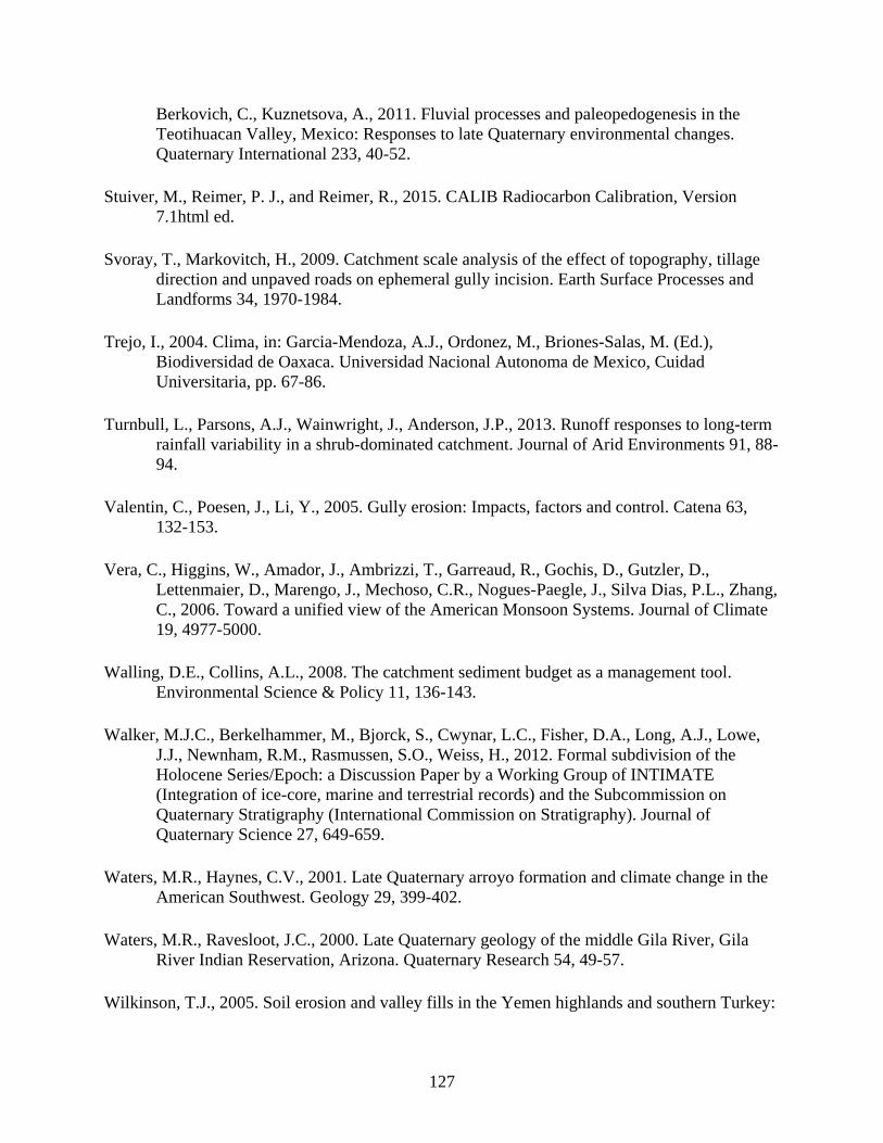
127
Berkovich, C., Kuznetsova, A., 2011. Fluvial processes and paleopedogenesis in the
Teotihuacan Valley, Mexico: Responses to late Quaternary environmental changes.
Quaternary International 233, 40-52.
Stuiver, M., Reimer, P. J., and Reimer, R., 2015. CALIB Radiocarbon Calibration, Version
7.1html ed.
Svoray, T., Markovitch, H., 2009. Catchment scale analysis of the effect of topography, tillage
direction and unpaved roads on ephemeral gully incision. Earth Surface Processes and
Landforms 34, 1970-1984.
Trejo, I., 2004. Clima, in: Garcia-Mendoza, A.J., Ordonez, M., Briones-Salas, M. (Ed.),
Biodiversidad de Oaxaca. Universidad Nacional Autonoma de Mexico, Cuidad
Universitaria, pp. 67-86.
Turnbull, L., Parsons, A.J., Wainwright, J., Anderson, J.P., 2013. Runoff responses to long-term
rainfall variability in a shrub-dominated catchment. Journal of Arid Environments 91, 88-
94.
Valentin, C., Poesen, J., Li, Y., 2005. Gully erosion: Impacts, factors and control. Catena 63,
132-153.
Vera, C., Higgins, W., Amador, J., Ambrizzi, T., Garreaud, R., Gochis, D., Gutzler, D.,
Lettenmaier, D., Marengo, J., Mechoso, C.R., Nogues-Paegle, J., Silva Dias, P.L., Zhang,
C., 2006. Toward a unified view of the American Monsoon Systems. Journal of Climate
19, 4977-5000.
Walling, D.E., Collins, A.L., 2008. The catchment sediment budget as a management tool.
Environmental Science & Policy 11, 136-143.
Walker, M.J.C., Berkelhammer, M., Bjorck, S., Cwynar, L.C., Fisher, D.A., Long, A.J., Lowe,
J.J., Newnham, R.M., Rasmussen, S.O., Weiss, H., 2012. Formal subdivision of the
Holocene Series/Epoch: a Discussion Paper by a Working Group of INTIMATE
(Integration of ice-core, marine and terrestrial records) and the Subcommission on
Quaternary Stratigraphy (International Commission on Stratigraphy). Journal of
Quaternary Science 27, 649-659.
Waters, M.R., Haynes, C.V., 2001. Late Quaternary arroyo formation and climate change in the
American Southwest. Geology 29, 399-402.
Waters, M.R., Ravesloot, J.C., 2000. Late Quaternary geology of the middle Gila River, Gila
River Indian Reservation, Arizona. Quaternary Research 54, 49-57.
Wilkinson, T.J., 2005. Soil erosion and valley fills in the Yemen highlands and southern Turkey:

128
Integrating settlement, geoarchaeology, and climate change. Geoarchaeology-an
International Journal 20, 169-192.

129
Figure 3.1. Map of study area. The map shows the location of
the study area including the Río Culebra, Inguiro and Verde
watersheds, along with the municipalities of Coixtlahuaca,
Nochixtlan, and Jicotlan (indicated by stars). The main map and
detail map show the location of the profiles in the study (black
triangles). Each profile is labeled as it is in the text. The general
location of the study area (black square) in the state of Oaxaca
(very dark gray) is shown in the inset map as well as the location
of the stalagmites from the Cueva del Diablo and Juxtlahuaca
caves in Guerrero (indicated by the two white circles and an
arrow on the inset map) (DEM data from USGS, 2015).
N
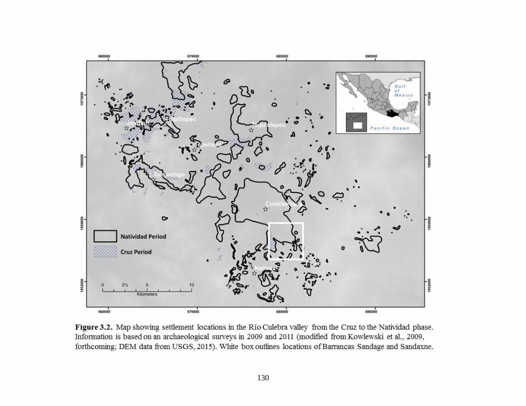
130

131
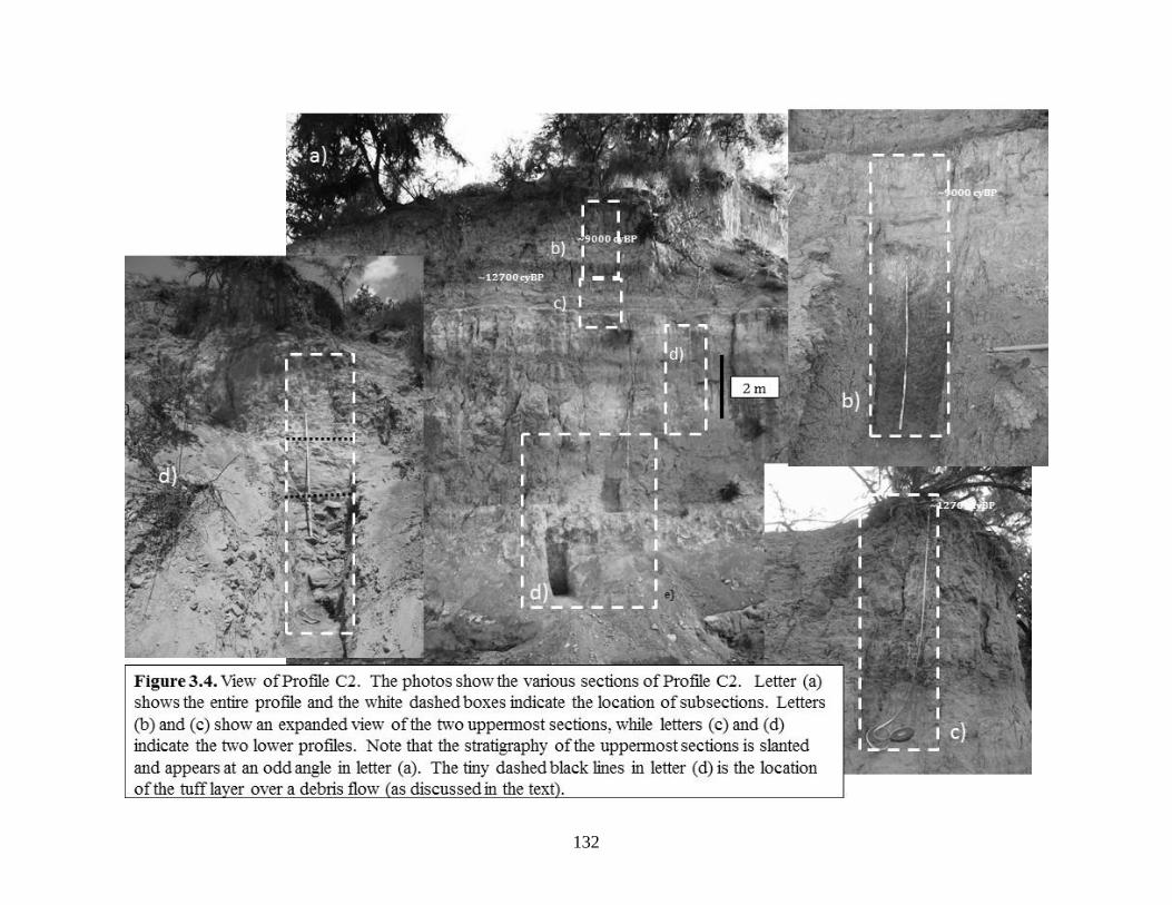
132
133
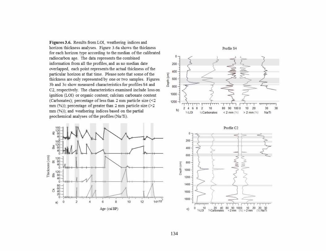
134

135

136
C.d.Diablo JX-10
JX-6 2012
JX-6 2013
JX-2
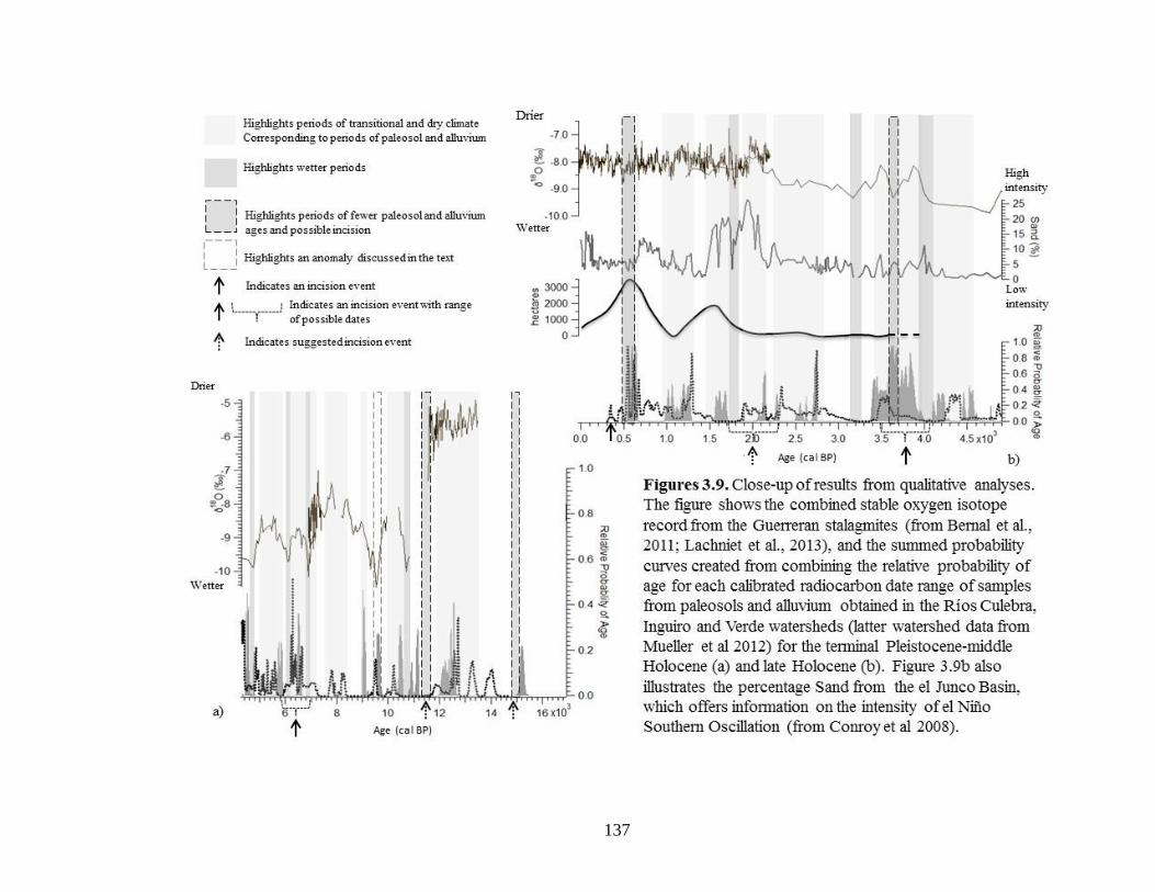
137

138

139
Table 3.1. Cultural phases of the Mixteca Alta. The corresponding Mesoamerican cultural period in both BP and BC/AD
ages are also shown (modified from Kowalewski et al., 2009).
Mixteca Alta Cultural
Phases
Ages Mesoamerican Cultural
Periods
Natividad *700 A.D. – 1520 A.D.
(1250 - 430 BP)
Post-Classic
Transición/Las Flores 200 A.D. – 700 A.D.
(1750 – 1250 BP)
Transition/Classic
Ramos 300 B.C. – 350 A.D.
(2250 – 1750 BP)
late and terminal Formative
Cruz 1500 B.C. – 300 B.C.
(3450 – 2250 BP)
early and middle Formative
*Note: Population decreases significantly between Las Flores and Natividad phases at ~1,000 cal BP.

140
Table 2.2 Radiocarbon dates from the study area.
UGA1 LAB
# Profile Horizon
Midpoint
Depth
(cm)
Material 14C Age (+/-) 1 Stdev 2-sig cal
range2
Median
Age
18031 C1 C 600 charcoal 2150 20 2060-2300 2143
18030 C1 C 750 charcoal 10550 30 12421-12619 12533
9230 C2 Ab 222.5 soil 2060 25 1949-2114 2028
9229 C2 Ck 490 charcoal 8130 30 8999-9133 9063
8666 C2 Ab 997.5 soil 10813 33 12684-12750 12717
8651 C3 C 67.5 soil 1332* 24 1180-1130 1278
12644 C3 Ab 199 charcoal 370 20 321-499 447
8652 C3 C4 280 charcoal 598 24 542-651 605
12645 C3 Ab 366.5 charcoal 550* 25 521-633 552
12646 C3 C 415 charcoal 1060* 25 928-1050 961
8656 C3 C 471.5 soil 1471* 24 1295-1515 1356
14628 C3 C 545 charcoal 1720* 25 1562-1698 1626
8657 C3 C 670 charcoal 1154 23 983-1152 1065
8658 C3 C 767.5 charcoal 1281 23 1181-1278 1234
8649 CFV C bottom of cut soil 5734 26 6451-6631 6527
8648 CFV Ab 992.5 soil 23529 64 27517-27829 27677
8661 I10 Ab 103.5 soil 1223* 23
14629 I10 Bwb 208 charcoal 1120 25 960-1166 1019
8660 I10 Ab 243 charcoal 1091 23 939--1057 996
8664 I10 C 470.5 charcoal 1964 24 1869-1987 1913
8663 I10 Ab 475.5 soil 1977* 25 1879-1949 1926
8662 I10 C 802.5 charcoal 3798 26 4039-4281 4183
12647 LB 175 ALLUVIUM 300 charcoal 5380* 25 6026-6279 6207
9224 LB 175 ALLUVIUM below wall charcoal 3370 25 3564-3689 3613
8643 LB 175 ALLUVIUM below wall charcoal 3384 26 3572-3692 3626
9226 LB 175 ALLUVIUM below wall charcoal 3430 25 3609-3822 3677
8650 LB 175 ALLUVIUM below wall organic
sediments 6783* 26 7587-7670 7631
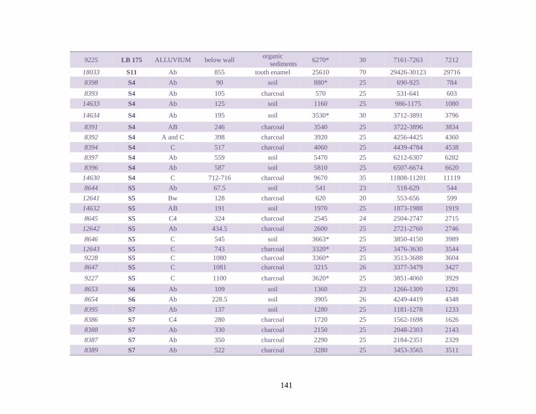
141
9225 LB 175 ALLUVIUM below wall organic
sediments 6270* 30 7161-7263 7212
18033 S11 Ab 855 tooth enamel 25610 70 29426-30123 29716
8398 S4 Ab 90 soil 880* 25 690-925 784
8393 S4 Ab 105 charcoal 570 25 531-641 603
14633 S4 Ab 125 soil 1160 25 986-1175 1080
14634 S4 Ab 195 soil 3530* 30 3712-3891 3796
8391 S4 AB 246 charcoal 3540 25 3722-3896 3834
8392 S4 A and C 398 charcoal 3920 25 4256-4425 4360
8394 S4 C 517 charcoal 4060 25 4439-4784 4538
8397 S4 Ab 559 soil 5470 25 6212-6307 6282
8396 S4 Ab 587 soil 5810 25 6507-6674 6620
14630 S4 C 712-716 charcoal 9670 35 11808-11201 11119
8644 S5 Ab 67.5 soil 541 23 518-629 544
12641 S5 Bw 128 charcoal 620 20 553-656 599
14632 S5 AB 191 soil 1970 25 1873-1988 1919
8645 S5 C4 324 charcoal 2545 24 2504-2747 2715
12642 S5 Ab 434.5 charcoal 2600 25 2721-2760 2746
8646 S5 C 545 soil 3663* 25 3850-4150 3989
12643 S5 C 743 charcoal 3320* 25 3476-3630 3544
9228 S5 C 1080 charcoal 3360* 25 3513-3688 3604
8647 S5 C 1081 charcoal 3215 26 3377-3479 3427
9227 S5 C 1100 charcoal 3620* 25 3851-4060 3929
8653 S6 Ab 109 soil 1360 23 1266-1309 1291
8654 S6 Ab 228.5 soil 3905 26 4249-4419 4348
8395 S7 Ab 137 soil 1280 25 1181-1278 1233
8386 S7 C4 280 charcoal 1720 25 1562-1698 1626
8388 S7 Ab 330 charcoal 2150 25 2048-2303 2143
8387 S7 Ab 350 charcoal 2290 25 2184-2351 2329
8389 S7 Ab 522 charcoal 3280 25 3453-3565 3511
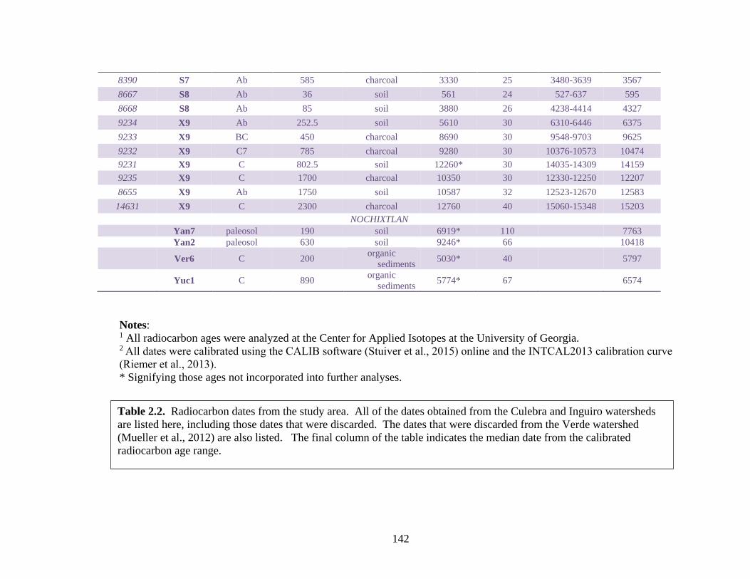
142
Notes: 1 All radiocarbon ages were analyzed at the Center for Applied Isotopes at the University of Georgia. 2 All dates were calibrated using the CALIB software (Stuiver et al., 2015) online and the INTCAL2013 calibration curve
(Riemer et al., 2013).
* Signifying those ages not incorporated into further analyses.
8390 S7 Ab 585 charcoal 3330 25 3480-3639 3567
8667 S8 Ab 36 soil 561 24 527-637 595
8668 S8 Ab 85 soil 3880 26 4238-4414 4327
9234 X9 Ab 252.5 soil 5610 30 6310-6446 6375
9233 X9 BC 450 charcoal 8690 30 9548-9703 9625
9232 X9 C7 785 charcoal 9280 30 10376-10573 10474
9231 X9 C 802.5 soil 12260* 30 14035-14309 14159
9235 X9 C 1700 charcoal 10350 30 12330-12250 12207
8655 X9 Ab 1750 soil 10587 32 12523-12670 12583
14631 X9 C 2300 charcoal 12760 40 15060-15348 15203
NOCHIXTLAN
Yan7 paleosol 190 soil 6919* 110 7763
Yan2 paleosol 630 soil 9246* 66 10418
Ver6 C 200 organic
sediments 5030* 40 5797
Yuc1 C 890 organic
sediments 5774* 67 6574
Table 2.2. Radiocarbon dates from the study area. All of the dates obtained from the Culebra and Inguiro watersheds
are listed here, including those dates that were discarded. The dates that were discarded from the Verde watershed
(Mueller et al., 2012) are also listed. The final column of the table indicates the median date from the calibrated
radiocarbon age range.
143
CHAPTER 4
STABLE CARBON ISOTOPE ANALYSIS OF ALLUVIAL PALEOSOL ORGANIC
MATTER IN THE MIXTECA ALTA, OAXACA, MEXICO3
3 Holdridge, G. and D.S. Leigh. To be submitted to Geoarchaeology.

144
Abstract
We examine δ13C values from soil organic matter (SOM) from the Culebra, Inguiro and
Verde watersheds (the latter was studied by Mueller et al., 2012) located in the Mixteca Alta
from the terminal Pleistocene to the present. In sum, the relatively depleted terminal
Pleistocene-early Holocene δ13C values suggest that C3 vegetation was more common than C4
and Crassulacean Acid Metabolism (CAM) vegetation, while the middle Holocene δ13C values
are enriched and suggest the prevalence of C4 and CAM relative to C3 plant biomass. The late
Holocene stable carbon isotope values vary, but in general they suggest slightly more C3 versus
C4 and CAM plant biomass than the previous period. The SOM δ13C values were compared
against the local paleosol data, and other paleoclimatic and paleoenvironmental proxies from
central and southwestern Mexico (e.g., Metcalfe et al. 2000; Caballero et al., 2010; Lachniet et
al., 2013). It was found that the terminal Pleistocene through the middle Holocene
paleovegetation of the watersheds in the study area reflects generally accepted changes in
paleoclimate. Similar to findings in central Mexico, the paleoenvironment of these watersheds
was impacted by human activities, such as agriculture during the late Holocene that affected
vegetation and caused erosion. Values of δ13C show a significant rise between 3,500 cal BP and
1,250 cal BP, with one notable cluster of enriched values corresponding to the Post-Classic
cultural period (local Natividad phase, 1,250-500 cal BP), when the population surpassed
100,000. Since the late Formative period (local late Cruz phase, starting ~3,500 cal BP), lama-
bordo (i.e., sediment check-dams) and agricultural terrace constructions were important for land
use management and agriculture, which became widespread by the Post-Classic period. The

145
highly enriched values associated with widespread agricultural structures suggest the increased
importance of maize cultivation during the late Holocene.
4.1 Introduction and Background
Paleosols are important because they provide a local source of information concerning
past environmental conditions. Stable carbon isotopes from soil organic matter (SOM), in
conjunction with paleosol studies and radiocarbon dates have been useful in indicating the
timing of vegetation changes in the late Quaternary (Cerling et al., 1989; Driese et al., 2005;
Hall and Penner, 2013; Coe et al., 2014). δ13C values vary within plants, and thus in SOM for
several reasons including: 1) atmospheric (CO2) and climatic factors (precipitation and
temperature) (Cerling et al., 1989); 2) physiographic factors (e.g., latitude and altitude); 3) and
genetic diversity among plant varieties (Tieszen, 1991). Plant biomass and associated isotopes
are especially sensitive to changes in paleoclimatic conditions in semi-arid and arid
environments subject to water-stress and temperature fluctuations (Amundson et al., 1994;
Ortega-Rosas et al., 2008). In some cases, analyses on bulk soil organic matter have the
potential to offer evidence of landscape disturbance associated with agricultural activity (de
Rouw et al., 2015), or more direct evidence, such as the past planting of maize (Johnson et al.,
2007; McClung de Tapia and Adriano-Moran, 2012).
Measuring the δ13C isotopic values of SOM offers information about past vegetation
composition (Cerling et al., 1989). Variations in the δ13C values in SOM reflect the values of
the original plant community, which are different for C3, C4, and Crassulacean Acid Metabolism
(CAM). The δ13C value of C3, C4, and CAM results from diverse fractionation associated with

146
different photosynthetic pathways (Farquhar et al., 1989; Tieszen, 1991; Boutton et al., 1998).
C3 plants follow the Calvin-Benson photosynthetic pathway, C4 plants use the Hatch-Slack
Cycle (Leavitt et al., 2007), while CAM follows a variation of the C4 pathway (Keeley and
Rundel, 2003). Values are determined by comparing the 13C/12C ratio to a standard, which is
typically the Pee Dee Belemnite fossil formation (PDB) (Farquhar et al., 1989).
The resulting differences between the 13C/12C and standard reflect these fractionation
and metabolic variations, though these processes and resulting values may overlap. In general,
typical isotopic values for C3 plants range from -22 to -32 per mil, those for C4 plants range
from -9 to -17 per mil, and those for CAM range from -10 to -30 per mil (Boutton et al., 1998;
Osmond et al., 1973). Depending on the environment, CAM may overlap significantly with
either C4 or C3 species in terms of their δ13C value, (Keeley and Rundel, 2003). The
intermediate values of CAM reflect their flexibility; for example, if the δ13C values are closer to
the C4 range, it implies primarily nocturnal carbon intake, whereas if values are more depleted
and similar to C3 biomass, it suggests that environmental conditions favored more direct cycling
of CO2 (Farquhar et al., 1989; Bhagwat, 2005). Unfortunately, it is thus far impossible to
distinguish CAM from C4 and C3 ratios based on δ13C values alone. A study in Baja California
on modern SOM δ13C showed that enriched δ13C values reflected greater percentage of CAM
biomass in locations with increasing summer precipitation, rather than alternating
photosynthetic adaptations of this plant type (Amundson et al. 1994). Both C4 and CAM plants
have been interpreted together due to their common adaptive strategies, which are advantageous
over C3 plants in low CO2, and drier and warmer climatic conditions.

147
Analyses of SOM should reflect the original average value of the vegetation, but organic
matter is heterogeneous in soil and sediment (Coe et al., 2014). Some difference between the
actual vegetation and the SOM values exists because it takes time for decomposing organic
matter to become integrated into the soil, which may alter the δ13C SOM values. The rate at
which the change in isotopic values occurs is related to the rate at which the soil organic matter
decomposes, and is referred to as the soil organic matter residence time or turnover rate
(Boutton et al., 1998). Some studies have actually preferred SOM in modern surface soils as an
indicator of present C3 versus C4 biomass because it represents the average of carbon inputs
over a number of years (von Fischer et al., 2008).
Changes in temperature, precipitation and atmospheric CO2 affect the amounts of C3
versus C4 and CAM plants in the landscape (Cerling et al., 1997; Huang et al., 2001). Both C4
and CAM plants have an advantage over C3 plants in dry, hot and/or saline environments (Sage,
2005). One of the main reasons for this advantage is linked to a mechanism of C4 and CAM
plants that fixes atmospheric CO2 more efficiently (Ehleringer, 2005). Photorespiration
involves the enzyme rubisco, which fixes CO2 in all plants. In C3 plants, air enters the stomata
by diffusion and either CO2 or O2 can be fixed; however, if the plant metabolizes oxygen it
results in photorespiration or the loss of CO2 and energy. The amount of oxygen metabolized is
a function of the O2/CO2 atmospheric ratio and temperature. High temperature increases the
fixation of oxygen and decreases the light-use efficiency in C3 plants. Conversely, C4 plants
avoid photorespiration by converting CO2 into a four-carbon molecule and moving it into an
internal compartment commonly known as the bundle sheath tissue, where it is concentrated
around rubisco (Ehleringer, 2005; Sage, 2005). At cooler temperatures, C3 plants assimilate

148
more CO2 relative to C4 plants, and thus the former has the competitive advantage. Conversely,
higher temperatures (i.e., 35°C or above) favor C4 plants because they reduce CO2 assimilation
and increase photorespiration losses in C3 plants. Therefore, temperature is often a dominant
factor (after CO2) in determining or reflecting C3 vs C4 productivity (Ehleringer, 2005; von
Fischer et al., 2008; Sage, 2008).
CAM plants are similar to C4 in that they can also concentrate CO2 where photosynthesis
occurs, though via a different mechanism. Typically CAM plants absorb and store CO2
biochemically during the night, and process it during the day with closed stomata, which also
ensures water conservation (Ehleringer, 2005). CAM plants are limited because they need
sufficient light and space to grow, and thus they cannot outcompete the faster turnover/growth
of C4 in similar environmental conditions (Keeley and Rundel, 2003).
Precipitation and moisture also affect photosynthetic pathways in plants in conjunction
with CO2 and temperature. In water-stressed environments all plants must close their stomata to
reduce water loss, reducing assimilation of CO2, but this especially occurs in C3 plants (Sage,
2005). In general, low water, low humidity and/or high salinity increase photorespiration in C3
vegetation, making dry and/or saline climates disadvantageous to C3 versus C4 and CAM plants
(Ehleringer, 2005; Sage, 2005). However, in high CO2 conditions and relatively moderate
temperatures the stress on C3 plants and photorespiration is not enough to counteract their
survival, even in very dry or saline conditions (Sage, 2005). Notably, C4 plants do not have any
morphological modifications to avoid water loss per se (Boom et al., 2001), whereas CAM
plants maximize water retention efficiency by closing their stomata during the day (Keeley and
Keeley, 1989). Variability in rainfall amount and inter-annual rainfall occurrence appears very
149
important in conjunction with growing season temperature and CO2 to influence the resulting
dominant plant type in present day environments (Shaw et al., 2005). Average temperature
during the wet or growing season is linked to differentiation in pathways, whereby C4 and CAM
plants are prevalent in summer rain regimes, and C3 plants dominate in winter rain regimes
(Ehleringer, 2005).
4.1.1 Objectives
In this paper we explore the late Quaternary paleoenvironmental changes in the Mixteca
Alta in south-central Mexico as reflected in the δ13C values from SOM. Stable carbon isotope
data from paleosols will be presented from the Río Culebra watershed in Coixtlahuaca and
Nativitas municipalities, and will include data from one profile along the Río Inguiro basin in
Jicotlan. The study will also include data from the Río Verde watershed in Nochixtlan studied
by Mueller et al. (2012). The δ13C values from SOM represent changes in paleovegetation over
the last 16,000 years. Many of the δ13C values were obtained from numerically dated
(primarily radiocarbon dating) organic matter within buried A horizons (these samples will be
referred to as dated buried A SOM samples) from profiles examined in the Culebra, Inguiro and
Verde watersheds. Other samples were obtained from undated organic matter in buried A
horizons (these samples will be referred to as interpolated buried A SOM samples), and their
ages were estimated using linear interpolation from other dates in the same profile (see
Methods). Analyses of isotope values and descriptive properties of paleosols will be used as
proxies for the local paleoenvironmental signal. This local signal will be compared to pre-
existing studies of paleoclimate data from stalagmites in the nearby state of Guerrero (Bernal et
al., 2011; Lachniet et al., 2013), regional changes in pollen, diatom and lake levels in central

150
Mexico (e.g., Metcalfe et al., 2000; Caballero et al., 2010), and overall changes in global
atmospheric CO2 as recorded in the Antarctic ice cores (Monnin et al., 2001; 2004). The main
objectives of this study are twofold: 1) to determine if the δ13C values from SOM are non-
randomly distributed throughout the late Quaternary and possibly related to atmospheric and
climate changes; and 2) to determine if non-random changes correspond to the prevailing
knowledge of regional paleoenvironmental fluctuations and/or human manipulations of
vegetation in the late Holocene (i.e. maize agriculture).
4.2 Study Sites
Data were collected from stratigraphic sections within deep gullies, locally known as
barrancas, in the Río Culebra watershed, located in the municipalities of Coixtlahuaca and
Nativitas (roughly 17° 43’N and 97° 19’W and 17° 27’N and 97° 13’W, respectively) and the
Inguiro watershed in the municipality of Jicotlan (approximately 17° 27’N and 97° 13’W)
(Figure 4.1). The study area is located in the Mixteca Alta, Oaxaca, Mexico, which is a sub-
region of the Mixteca physio-cultural region in northern Oaxaca (see Balkansky et al., 2000).
The Mixteca Alta lies approximately 2300 m amsl (above mean sea level) in the Sierra Mixteca,
which is one of the sub-ranges of the Sierra Madre del Sur (Krasilnikov et al., 2013).
The high terrain of the Sierra Madre del Sur bordering the basin causes a rain shadow in
the region. The North American Monsoon is the source of most precipitation in the region, the
timing and duration of which is predominantly controlled by the movement of the Intertropical
Convergence Zone (ITCZ), and the intensity of the El Niño Southern Oscillation (ENSO)
(Trejo, 2004). The region is characterized as a semi-arid climatic regime (BSh Köppen
151
classification), averaging around 528 mm of rain per year, with an average annual temperature
range between 13.2-18.6 ºC (Servicio Meteorologico Nacional, 2010). The warmest time of the
year overlaps with the rainy season, which spans May through October, with peaks in June and
September.
The geology of the study area predominantly consists of lower to middle Tertiary
siltstones and claystones (shales), referred to as the Yanhuitlan Formation, which precede minor
outcrops of middle Tertiary volcaniclastics and andesites (Santamaria-Diaz 2008). Quaternary
alluvium fills much of the main valleys of the Ríos Culebra and Inguiro as well as their
tributaries. These dryland streams have incised about 7 m to 35 m down into the Quaternary
alluvium. A study of soils in the Coixtlahuaca District (Sánchez, 2004) indicated that 46% of
the soils consist of Aridisols, 49% of the soils are Mollisols (or more specifically Rendolls), and
the remaining 5% fall under Alfisols, Entisols, and Vertisols. The majority of the soils are
associated with calcareous parent materials (Sánchez, 2004). Many of the hillslopes in the
Mixteca have exposed calcrete surfaces, and both hillslopes and valley alluvium exhibit
widespread barranca development (Rincon, 1999; Leigh et al., 2013). Another study by the
National Institute of Statistics and Geography (INEGI, 2005) in Mexico indicates that Entisols,
Vertisols and Mollisols are the primary soil types in the municipalities of Coixtlahuaca,
Nativitas and Jicotlan.
The land cover (Figure 4.2) within the Culebra, Inguiro, and Verde watersheds primarily
consists of human-induced pastureland, agricultural land and secondary vegetation, along with a
small amount of urban land. Both Culebra and Verde watersheds also contain some bare
ground and chaparral. The chaparral includes spiny and schlerophyllis scrubland (e.g.,

152
rosetofilous desert scrub). Primary forests are composed of mainly live oak, pine, and juniper,
while secondary vegetation consists of juniper, oak and pine scrublands (Colín, 2004; INEGI
landcover data, 2013). Recently, pine trees have been planted to reforest some bare hillslopes in
an effort to reduce erosion (Rafael Arzate Aguirre, pers. Com.).
4.3 Methods
Stable carbon isotope analyses were conducted on the SOM from buried A horizons
using profiles described and sampled in alluvium located in the Río Culebra and Río Inguiro
valleys, as reported in Chapter 3. For the profiles C2, C3, S1 through S8, I10, and X9, one or
more radiocarbon dates on charcoal or SOM from buried organic horizons offered ages for the
strata in the profile. Some of the δ13C values incorporated into this study were from the
radiocarbon dates made on preserved buried A horizons, sampled within 5-10 cm of the
boundary to overlying horizons. A total of 13 δ13C values were obtained from the upper portion
of these buried A horizons. All radiocarbon dates from charcoal and SOM from buried A
horizons were calibrated using the online CALIB software (Stuiver et al., 2015) and the
INTCAL13 calibration curve (Reimer et al., 2013).
Another 20 samples of buried A SOM samples were directly analyzed for percent total
organic carbon (%TOC) and δ13C but were not directly dated. Samples were obtained on the
upper part of the buried A horizons, 10-25 cm from the boundary with the horizon above, from
the following profiles: C1, C2, S4, S11, X9, and I10. Analyses were made on these profiles to
observe changes in δ13C according to depth and to determine the reproducibility of the isotopic
signature in the SOM from this region. The ages for these δ13C values from buried A SOM were
153
interpolated using the Classical Age Model (CLAM) of Blaauw (2010, version 2.2) with R
software (R Core Team, 2013).
The δ13C data from 20 buried A SOM samples from Río Verde (Mueller et al., 2012)
were combined with the data from Culebra and Inguiro for further study. The δ13C data from
charcoal samples (18 samples in total) from buried A horizons were also included for initial
comparison to the SOM from buried A horizons. Finally, SOM from modern soils were
gathered from within 20 cm from the surface, in 10 cm increments. The modern samples were
obtained from four representative field sites, representing various vegetation cover including
grass, scrub, mixed, and forested (Table 4.1).
Radiocarbon dating and stable carbon isotope analyses were performed in the Center for
Applied Isotopes (CAIS) at the University of Georgia. For radiocarbon dating, charcoal and
soil samples from Culebra and Inguiro watersheds were soaked in 1N HCl at 80°C for 1 hour,
then washed with deionized water on a fiberglass filter, and rinsed with diluted NaOH to
remove possible contamination by humic acids. Next, the sample was soaked in 1N HCl again,
washed with deionized water and dried at 60°C. For the accelerator mass spectrometry analysis,
the cleaned sample was combusted at 900°C in evacuated and sealed ampoules in the presence
of CuO. The resulting carbon dioxide was cryogenically purified from the other reaction
products and catalytically converted to graphite using the method of Vogel (Vogel et al., 1984).
Graphite 14C/13C ratios were measured using the CAIS 0.5 MeV accelerator mass spectrometer,
and these ratios were compared to the ratio measured from the Oxalic Acid I (NBS SRM 4990).
The sample 13C/12C ratios were measured separately using a stable isotope ratio mass
spectrometer and expressed as δ13C with respect to PDB, with an error of less than 0.1‰.

154
For stable carbon analyses of SOM in paleosols and surface soils, the samples were
heated overnight at 105°C to remove any excess water, weighed, and then soaked in 1N HCl
while heated overnight in a fume hood at 60°C. A drop of 1N HCl was then added to ensure the
complete removal of carbonates, and the samples were dried again overnight at 60°C in a
separate oven. Due to the small amount of organic carbon in the samples, they were not rinsed,
but subsamples were weighed and placed in silver cups in final preparation for analysis. Next,
the samples were analyzed in an elemental analyzer-stable isotope ratio mass spectrometer and
expressed as δ13C with respect to PDB, with an error of less than 0.1‰ (as above). Since the
samples were not rinsed, and the sample size of the interpolated SOM analyzed was initially
small, the percentage of total organic content was very small or registered below the detection
limit of the elemental analyzer in other cases. Therefore, 12 of the 24 samples were run a
second time using a larger amount of the prepared SOM sample to better determine or verify
their δ13C value (Table 4.1).
Other studies have incorporated the δ13C values from radiocarbon dates along with
samples analyzed specifically for SOM in buried As (e.g., Hall and Penner, 2013). It was
determined that the two sets of δ13C values are comparable because the δ13C values were
obtained from the total organic carbon rather than from a portion of the SOM carbon (i.e.,
humic acid). Furthermore, the standard preparation for radiocarbon dating is more rigorous
than the standard procedure typical of δ13C analysis. Replications involved re-analyzing the
same paleosol SOM samples using the same pretreatment to observe how the resulting δ13C
values compared. We also compared the δ13C values of three paleosols using both pretreatment
approaches. Results are presented in Table 4.1 and discussed below.

155
4.3.1 Soil Residence Time and Interpolated Dates
The organic matter from many paleosols in the Coixtlahuaca region have been shown to
be older than dates from charcoal, which may be due to the incorporation of older detritus,
including charcoal or older SOM, and/or may be related to the long residence time of the soil
(dry conditions, slow decomposition) (Rincon, 1999; Leigh et al., 2013). Although it is known
that charcoal is inherently older than the soil or sediment in which it is found (Leigh et al.,
2013), after examining the dated profiles, charcoal is more consistent with regard to depth as
compared to buried A SOM dates (Chapter 3). Five pairs of dates, each consisting of a charcoal
date paired with a buried A SOM date from the same strata (taken from Rincon, 1999 and Leigh
et al., 2013) were compared to estimate the average inconsistency of the buried A SOM dates.
All of the dates were calibrated using CALIB (see above for references). The difference
between the calibrated range for each individual sample was examined against the differences
between the calibrated ages of the charcoal and organic samples from the same strata (see
Appendix III). The calibrated range for each individual sample was comparable to the
differences between the calibrated ages of the charcoal and organic samples from the same
strata. The seemingly erratic nature in which the organic material may incorporate older
detritus means that, based on the available data, no single correction factor can account for the
all of the variation in soil ages. In sum, it was concluded that the median of a calibrated date
was a reasonable estimate of the age of a stratum after considering the relationship between the
ages along the depth of a profile.
4.3.2 Surface Samples
Four modern surface samples were collected from the Culebra watershed and one from
156
the headwaters of the Río Grande (see Figure 4.1 for location). The samples were selected to
represent forest (Apo): grassland (with a few scattered trees) (Ast): mixed grassland and
succulent plants (Vic1): and mixed grassland, succulent and forest (Vic2). The sites with forest
(e.g., Apo and Vic2) were taken from hilltops and not on the bottomland alluvium because
presently trees are mainly preserved at the top of hillslopes. The sites were selected to be
representative of vegetation types, and no site represented a perfectly homogenous or mixed
site. The samples were collected by obtaining the top 20 cm (in 10 cm intervals) every 25
meters across a transect of 50 meters, for a total of six samples per transect. The final analyses
were conducted on a mixed composite of all 0-10 cm samples within each transect for a total of
four surface samples. Two modern samples originally taken to double check the radiocarbon
dates from buried A SOM were also incorporated into the results. These samples come from
surface soils under mixed grassland and succulent vegetation.
Any modern value will be influenced by the rise of fossil fuels in the last 200 years and
the influx of ‘old’ CO2 (e.g., δ13C depleted) into the atmosphere known as the Suess effect
(Suess, 1955; Brook et al., 2015). Values are typically depleted between 1.5‰ (Boutton et al.,
1998; Wynn and Bird, 2008) and 2.0‰ (Brook et al., 2015), though the former amount has been
observed in soils (Boutton et a., 1998; Wynn and Bird, 2008). An additional 1.5‰ was added to
the resulting δ13C values from the modern analyzed soil organic matter (Table 4.2).
4.3.3 Percentage C4 plants
Boutton et al. (1998) developed a mass balance equation (formula (a)) for a subtropical
savanah ecosystem, which was applied to this study to estimate the amount of C4 biomass in the
paleoenvironment based on the δ13C values (as in Biedenbender et al., 2004; Lounejeva

157
Baturina et al., 2006). Formula (b) (Kelly et al., 1998) shows how the δ13C values were used to
calculate the percentage C4 biomass in the study area. Since CAM in the region is important but
cannot be distinguished from C4 based on δ13C values alone, the resulting calculated percentage
will be assumed to represent both C4 and CAM.
These formulas are given as follows:
δ13Cmeas = x(δ13C4) + (1-x)( δ13C3) (a), and
%C4 = (δ13Cmeas - δ13C4)/(δ13C4 - δ13C3) (b),
where δ13Cmeas indicates the measured value from the SOM, δ13C3 represents the average value
of modern day C3 plants in the region, and δ13C4 is the average value of present CAM and C4
plants in the region. The present values of C4 and C3 plants were estimated from a study done
on floral isotopic diversity of highland Oaxaca by Warinner et al. (2013), which focused on
wild and cultivated plants typically used by inhabitants. The average δ13C3 and δ13C4 values
obtained for highland Oaxaca vegetation were estimated from analyses on 150 wild plants
collected in transects, and found to be -28 and -13.3 per mil respectively. Estimated δ13C for
wild CAM plants were similar to the δ13C4 values (e.g., ~14.3 per mil) (Warinner et al., 2013).
Though CAM values are slightly lower, overall the study found that 80% of CAM δ13C values
were similar to C4 plants (Warinner et al., 2013). As discussed in 4.3.2, due to the Suess effect
(Suess, 1955; Wynn and Bird, 2008; Brook et al., 2015), an additional 1.5‰ was added to the
modern δ13C values used in the formula above (see Table 4.3).

158
4.4 Results
A total of 38 stable carbon isotope values came from the Culebra and Inguiro
watersheds, listed as follows (summarized in Table 4.1): 13 values were obtained on dated
buried A SOM, 20 values came from interpolated buried A SOM, six values came from
analyses on modern SOM, and 18 values were obtained from dated charcoal samples.
Altogether 20 stable carbon isotope values from dated buried A SOM were incorporated into
this study from the Río Verde watershed (see Mueller et al., 2012).
Table 4.1 summarizes δ13C values from the Ríos Culebra and Inguiro. Three dated
buried A SOM samples, which already had δ13C values associated with the radiocarbon date,
were re-analyzed to determine the replicability of the dated buried A SOM stable carbon isotope
results. In two of the cases the values were slightly enriched (comparable within 0.56 per mil),
while the other sample was enriched by 2.2 per mil and clearly differed. It is possible the latter
contained a fleck of charcoal that caused the value to increase. Some of the interpolated SOM
samples were also re-analyzed due to small sample size, and resulting small %TOC, in order to
double check the initial δ13C value results. In all of these cases the second analysis, having a
bigger sample size, produced δ13C values that were within less than 1.65 per mil of the initial
results. The averaged δ13C value of the two analyses was accepted as the final value. In a few
cases the small sample size produced a %TOC value that was below the detection limit of the
elemental-analyzer and the initial δ13C values were removed. Only the value from the second
analysis was accepted. If a strata contained both an interpolated and a dated buried A SOM
δ13C value, the two values were averaged, and this averaged δ13C value was accepted as the
final value.

159
The percentage of total organic carbon (%TOC) obtained for the interpolated buried A
SOM is presented in Table 4.2. In cases when the samples were analyzed twice, the %TOC
represents the average value if the δ13C values were averaged, and the re-analyzed value in the
cases where only the δ13C value from the second analysis was accepted. Similar to other
studies, it was found that %TOC decreased with regard to depth (Figure 4.3a). Stable carbon
isotope values were examined with respect to depth (Figure 4.3b) and it was found that there
was no apparent pattern, but other studies have shown that a slight enrichment of δ13C values
may occur with depth, resulting in approximately a 2 per mil increase in values (Wynn, 2007).
The δ13C values for all three watersheds range from -26.73 per mil to -15.7 per mil. The
general trend in values, as ascertained from the mean and standard deviation of each period
(Figure 4.4), shows more depleted values in the terminal Pleistocene through the early
Holocene, more enriched values in the middle Holocene, and more depleted values in the late
Holocene as compared to the middle Holocene. The range in δ13C values of the terminal
Pleistocene-early Holocene is -26.54 to -16.7, while the middle Holocene δ13C values have a
range of -24.49 to -16.1. The range of the late Holocene is -22.2 to -15.7. A closer look at the
δ13C values from all three watersheds indicates that some values appear to be outliers (Table 4.1
and Figure 4.4). All of the outliers came from the interpolated buried A SOM samples from site
C2 in Culebra watershed, and the dated buried A SOM samples from sites Yuz9 and Ver6 in
Río Verde.
The δ13C values from the Culebra, Inguiro, and Verde watersheds are plotted against age
(Figure 4.5), and it is apparent that the charcoal samples from the Culebra and Inguiro
watersheds are consistently more depleted than the rest of the samples. The more depleted

160
values are expected since charcoal is derived primarily from trees (C3 vegetation). Thus, the
charcoal samples were not considered good representatives of landscape-scale vegetation
patterns.
If examined apart from the late Holocene, the modern δ13C values are the most depleted,
even after considering the Suess effect. Altogether these come from six surface soil samples,
four of which were directly analyzed for their stable carbon isotope value. The δ13C values
from the other two samples came from radiocarbon dating, which were used as a double check
on the radiocarbon dates from SOM in buried A horizons (Chapter 3). Of the four modern
categories analyzed, the δ13C value for the modern forest (Apo) is the most depleted (-25.23).
The modern value for grassland (Ast) is the most enriched at -20.89, but is still relatively
depleted suggesting the dominance of C3 grasses. The mixed forest (Vic2) δ13C value is slightly
more depleted (-24.18) than the mixed grassland (Vic1) (-21.84). The two dated samples of
mixed grassland and succulent plants obtained values of -19.92 and -22.25, both of which are
closer to mixed grassland and grassland values than mixed forest values. The average δ13C
value for all of the modern samples is -22.39, and the difference between highest and lowest
value is 5.31 per mil, which equates to a difference in 36% of C4 and CAM vegetation.
4.4.1 Calculated %C4 and CAM
Enrichment of stable carbon isotope values was interpreted to indicate an increase of C4
and CAM biomass in relation to C3 plants (and is the opposite for depleted values) (e.g.,
Lounejeva Baturina et al., 2006; McClung de Tapia and Adriano-Moran, 2012). Typically, an
increase in C3 vegetation (e.g. indicated by depleted values) implies a wetter and/or cooler
161
climate, whereas an increase in C4 and CAM biomass (e.g., indicated by more enriched values)
is associated with an increase of dry and/or warm conditions.
The calculated percent of C4 and CAM biomass is presented in Table 4.4. Incorporating
all profiles, variability was high at times and is reflected in the calculated %C4 and CAM for
individual values with overlapping ages (refer to both Tables 4.1 and 4.4). For example,
median ages of 9,554, 9,751, and 9,833 cal BP (i.e., these ages contain overlapping calibrated
radiocarbon ages) resulted in an estimated %C4 and CAM of 24, 43, and 67%, respectively.
Variability in δ13C values averaged to represent the same time range was within 2-18%, if the
outlier values from profiles C2, Yuz9 and Ver6 (e.g., profiles with consistently lower δ13C
values) were removed. In general, the data is more useful when examined as a whole and to
discern general trends over time.
The averaged %C4 and CAM for the Terminal Pleistocene-early Holocene (~16,000-
8,200 cal BP) fluctuated within a range of 24-67%, having a median of 40% and a mean of
41%. The range in %C4 and CAM suggested it was overall wetter and/or cooler. The averaged
%C4 and CAM calculated for the middle Holocene (8,200 cal BP to 4,300 cal BP) ranges from
52-76%, with a median of 55% and a mean of 51%, indicating drier and/or warmer conditions.
The late Holocene (4,300 cal BP through 500 cal BP) averaged %C4 and CAM values range
from 56-63%, with a median of 46% and a mean of 49%, suggesting overall dry and/or warmer
conditions, but slightly moister and/or cooler than the middle Holocene. Widespread land use
activities may have also affected the δ13C values during the late Holocene, which will be
discussed below (see section 4.5 Discussion). The %C4 and CAM for more recent δ13C values
(e.g., 500 cal BP to present) is the lowest estimated, having an average of 28%. Despite the
162
present dry and warm climate, the modern δ13C values are very depleted, which may be linked
to present human impact.
4.4.2 Paleovegetation and CO2
Some authors have observed a relationship between δ13C values and both climate and
CO2 earlier in the Holocene (e.g., Huang et al., 2001; Urban et al., 2015). Prior to direct
measurements of CO2 in the atmosphere, estimations of past global atmospheric CO2 came from
trapped air bubbles in the Antarctic ice sheets. The CO2 value from the ice cores are considered
proxies for global CO2 in the past because the main source of CO2 is in the tropics, meaning the
value in the Antarctic is a result of the incorporation and mixing of the CO2 in the atmosphere
(Monnin et al., 2001; Monnin et al., 2004; Trudinger et al., 2005). In general, CO2 values
below 180 ppm are considered low enough to starve C3 plants of CO2, especially in conjunction
with stressful climatic conditions (Bhagwat, 2005). For example, values below 180 ppm
resulted in a reduction of C3 vegetation (forests shrink) and expansion of grasses (C4) during the
last glacial maximum (LGM) (Ehlringer, 2005). After the LGM, values do fluctuate, but no
values are recorded below 180 ppm (e.g., Holocene CO2 values range between 260-280 ppm);
therefore, only in conjunction with certain climatic conditions would CO2 values affect
paleovegetation ratios (as in Huang et al., 2001). In this study, there is no correlation between
δ13C values and CO2, implying the δ13C values reflect climatic variations, and possibly human
influences in the late Holocene. It is unclear if CO2 has impacted plant biomass in the last 100
years.
163
4.4.3 Local Polynomial Regression Analysis
To explore the general trends in C4 and CAM verses C3 vegetation from the terminal
Pleistocene to the present, we analyzed all of the δ13C values with a local polynomial regression
to determine the most significant trends in the data (Figure 4.6). Analyses were done using the
LOESS (locally weighted scatterplot smoothing) function (Cleveland et al., 1992) in R software
(R Core Team, 2013). According to the analysis, the peak in the δ13C values during the middle
Holocene occurs around 7,000 cal BP, which is followed by a significant fall in values towards
4,900 cal BP. From 4,900 cal BP to 1,200 cal BP, the regression suggests that a significant
increase in C4 and CAM vegetation occurs during the late Holocene, which peaks between
1,000-500 cal BP. After this peak, there is a steady and significant decrease in values towards
the present, and is probably impacted by the more depleted modern values, which were
averaged to avoid bias. The peak around 1,000-500 cal BP and the subsequent fall in values is
significant, and coincides with the Natividad phase (1,250 – 500 cal BP) and Colonial period
(post 500 cal BP).
4.5 Discussion
The δ13C values and the calculated %C4 and CAM are examined with regard to present
and paleoenvironmental data. The results from the analyses assume that the samples are equally
representative of the surrounding environment, though it is realized that vegetation does vary
spatially. Increasing δ13C values in soil organic matter suggest more C4 and CAM biomass,
while more depleted values reflect more C3 vegetation (Amundson et al., 1994; Boutton et al.,
1998). However, variations can occur due to sub-sampling differences; for instance, one sub-

164
sample may contain more charcoal resulting in more depleted values. In addition, alluvial soils,
especially in arroyo stratigraphy, may contain organic content eroded from an older soil, which
upon mixing with a more recent soil may affect the resulting δ13C values. Finally, soil samples
associated with primarily riparian vegetation will produce δ13C values that represent this
biomass and not the vegetation of the watershed as a whole. Despite this potential bias, this
study contains a number of samples with overlapping ages and/or contexts, which reflect
general changes in trends of biomass overtime, whether influenced by climatic and/or land use
changes.
Since charcoal samples do not represent an integrated value of vegetation in soil organic
matter, they are not incorporated into more in-depth paleovegetation trends. However, charcoal
has been observed in a number of strata corresponding to different ages in the last 15,000 years,
suggesting the importance of trees, or C3 vegetation in the landscape during much of this
time. A notable exception is a period of more enriched δ13C values between around 9,000-
4,300 cal BP, when no charcoal samples were dated. This observation suggests that the
paleoclimatic conditions were not favorable to C3 vegetation, resulting in reduced C3 vegetation,
such as trees in the landscape.
4.5.1 Modern Soils
The present day vegetation of the municipalities of Coixtlahuaca, Jicotlan and
Nochixtlan is mainly induced and secondary vegetation and agricultural land. No studies have
been made on the distribution of plants with different pathways in the region, but based on some
of the known δ13C values of certain species in the region, it is certain that the present vegetation
comprises an uneven mixture of C3, C4 and CAM species.

165
Globally, drylands are experiencing an encroachment of woody vegetation (C3) into
grasslands (C4). A study on the Chihuahua Desert suggests that this change is influenced by
localized biogeophysical factors such as soil erosion, nutrient loss and reduced water
infiltration. Woody perennial species have higher soil moisture extraction capacity than C4
grasses. The expansion of these woody species results in the reduction of soil organic carbon
content and surface water infiltration (Albert, 2015). Some vegetation like chaparral, which is
normally found in Mediterranean climates (e.g., hot dry summer and cool, wet winters) is
observed in rain shadow regions of the Sierra Madre del Sur, and is a relic of the drying climate
in the Tertiary and adaptation to a long drought season (Valiente-Banuet et al., 1998).
Increasing secondary woody vegetation (C3) in the Culebra may result from the poor
management of the landscape such as deforestation and uncontrolled grazing (Rafael Arzate
Aguirre, pers. Com.).
Presently, CAM biomass is a significant part of the Mixteca Alta’s vegetation (Valiente-
Banuet, 1998; Colin, 2004; Blancas et al., 2010) and it probably had an important role in the
past 16,000 years. However, a study on the local management of the Biosphere Reserve
Tehuacán-Cuicatlán, which encompasses parts of Culebra and Inguiro watersheds, suggests that
some native and non-native plants, including native CAM plants, are considered useful and
better managed so are more abundant in the landscape than they would normally be (Blancas et
al., 2010). Present day CAM δ13C values in Oaxaca (Warinner et al., 2012), and in Baja
California are typically enriched (Amundson et al., 1994), which would not explain the more
depleted δ13C values found in modern soils in this study. More recently managed forests (via
government subsidies and management, Rafael Arzate Aguirre, pers. Com.) entail planting of

166
non-native pine trees (C3), which possibly influenced some of the modern δ13C values,
especially in Sandage.
Finally, studies have shown that CO2 affects the growth, survival and reproduction of
plants in arid/semi-arid environments. With no other limitations, elevated CO2 leads to greater
productivity (and usually favors C3 over the other two pathways), while local factors such as
water amount and temperature mediates the influence of CO2 (Shaw et al., 2005). In the last
200 years, the exponential rise in CO2 to over 400 ppm is the highest it has been in the last 10
million years, which favors C3 plants (Sage, 2005). In sum, higher erosion and other human
induced disturbances, natural occurrence of C3 woody species, and the rise in CO2 in the last
100 years would all favor an increase in C3 plants, and would help explain the depleted modern
δ13C values observed in this study.
4.5.2 Paleoenvironmental Reconstruction
The SOM δ13C values from Coixtlahuaca and Nochixtlan for the terminal Pleistocene to
the late Holocene were examined against local paleosol data (Mueller et al., 2012; Chapter 3),
paleoclimatic and paleoenvironmental data from southwestern and central Mexico (e.g.,
Metcalfe et al., 2000; Caballero et al., 2010; Lachniet et al., 2013), and other tropical sources
(e.g., Cariaco basin, Haug et al., 2001; El Junco Crater Lake, Conroy et al., 2008). The earliest
δ13C value had an age of approximately 15,800 cal BP, and thus we compare our values with
external data starting at 16,000 cal BP.
Paleoclimate data are represented by a qualitative summary (Figure 4.7) of the lake data,
glacial data, stalagmite data and δ13C data from this study (the latter includes δ13C values from
Mueller et al., 2012). However, the data are variable and contradictory, in particular the lake
167
data, making interpretation ambigious. Therefore, when raw data were available, z-scores were
calculatedin order to better discern overall trends in the paleoenvironment (Figure 4.8). The
figure description of Figures 4.7 and 4.8 contain all of the references included in this summary
by region and according to paleoclimate proxy.
Paleoclimate and paleoenvironmental proxies include pollen, diatom and δ18O data from
lake records from central Mexico, glacial studies from central Mexico, δ13C data from the
Cueva del Diablo stalagmite from Guerrero, and δ18O data from all studied Guerreran
stalagmites in southwestern Mexico. The stalagmite δ18O signature represents a high-resolution
reconstruction of paleoprecipitation data, while the paleolimnological and glacial data mainly
exhibit general trends over time. The δ13C values from the study area with overlapping
calibrated radiocarbon ages were averaged together and presented in Figure 4.7.
4.5.2.1 Terminal Pleistocene-early Holocene (~16,000-8,200 cal yr BP)
In general, the terminal Pleistocene-early Holocene transition encompasses some major
fluctuations corresponding to the Heinrich Stadial 1 (HS1), the Bølling-Allerod (B/A), the
Younger Dryas (YD), and the 10.3 ka event (Anderson et al., 2007).
The Guerreran stalagmites reflect these fluctuations with dry conditions during HS1 and
the latter part of the B/A, which are interrupted by a hiatus during the early part of the B/A
representing wetter conditions (Lachniet et al 2013). The z-score calculations for the Cariaco
Basin also indicate drier conditions in the YD. Pollen records indicate that cold and wet
conditions during HS1 shift to cold and dry conditions during the B/A in the Patzcuaro basin,
while colder and drier climate persists in the Upper Lerma basin during the HS1 and part of the
B/A. Pollen records indicate that the climate during HS1 and B/A was colder and wetter in
168
Puebla-Tlaxcala while in the Basin of Mexico colder and drier conditions prevailed. Diatoms
support the colder and drier climate in the latter basin. Additionally, glaciers start to expand
during the HS1 event, and are still in expanded positions throughout most of the B/A, implying
wetter and colder climate in higher altitudes.
Most pollen, diatom and stable oxygen isotope (lake) records indicate that the Younger
Dryas (YD, ~12,900-11,700 cal BP) was wetter and colder, which persists through the transition
to the early Holocene and until 9,500 cal BP. For example, the pollen data from the Guanajato
and Michoacán area suggest that the YD through the early Holocene transition was wetter and
colder, and stable oxygen isotope studies from this area also support a wetter environment.
Pollen records indicate wet and cold conditions up to around 9,500 cal BP in the Puebla-
Tlaxcala area and the Basin of Mexico. One exception includes the pollen record in the
Patzcuaro basin, where it is transitioning from dry and cold to wet and warm in the early
Holocene. Another exception is the diatom record from the Basin of Mexico, which indicates
dry and warm conditions since the end of the YD through 9,500 cal BP. In addition, the diatom
record in the Upper Lerma basin suggests wet and warm conditions during the YD to 9,500 cal
BP, while the pollen information for the early Holocene suggests dry and cold conditions until
9,500 cal BP. Glaciers seem to slow in growth during the YD, suggesting a cold but dry
climate. This slowed growth is followed by another expansion of glaciers in the early Holocene
between 11,000-9,500 cal BP, which is evidence for a return to wetter and cooler conditions.
The Guerreran stalagmites indicate dry conditions during the YD and 10.3 ka event, but a hiatus
during the early Holocene is suggested to represent wetter conditions.

169
All pollen and diatom records indicate warmer conditions by 9,500 cal BP. A return to
very wet conditions is observed in the δ18O record around 9,500 cal yr BP (Bernal et al., 2011).
Both wet and warm conditions can be connected to peak northern hemisphere insolation (Haug
et al., 2001). Conditions are also wetter in the Basin of Mexico and the Puebla-Tlaxcala area
starting around 9,500 cal BP according to pollen records. Diatom and pollen records from
Upper Lerma basin indicate warm and wet conditions, though after 9,500 cal BP, the pollen
suggests warm and dry conditions. Diatom records for the Puebla-Tlaxcala area indicate
conditions are dry and warm for the entire early Holocene. Dry and warm conditions are also
observed for pollen records from the Guanajuato and Michoacán area between 9,500-8,200 cal
BP, which transitions to wet and warm at the end of this timespan.
The δ13C data from SOM from western (Ferrand et al., 2014) and central Mexico
(Lounejeva Baturina et al., 2006; Sedov et al., 2010) suggest a cold and wet terminal
Pleistocene, which transitions into a drier and warmer early Holocene. Many of these
conclusions in the δ13C data are supported by other proxy data (e.g., phytoliths, paleosol studies
and micromorphology). The δ13C data from Culebra, Inguiro and Verde watersheds indicate
slightly enriched values in the B/A and more depleted values in the YD. The %C4 and CAM is
calculated as <41, suggesting slight dominance of C3 vegetation. According to the z-scores, the
δ13C values from the study area are also depleted during the early Holocene except for a small
peak (and correspondingly, a slight increase in %C4 and CAM vegetation) around 10,000-
10,200 cal BP. A similar pattern is observed in the δ13C values from the Cueva del Diablo
stalagmite, but the small peak in enriched values occurs around 10,200 cal BP.

170
Paleosol studies on the Culebra, Inguiro and Verde watersheds indicate fluctuating
conditions. In general, the terminal Pleistocene and early Holocene paleosols consisted of
cumulic A horizons, contained clear calcium carbonate deposits ranging from nodules to
deposits in root pores and ped faces, and many horizons exhibited prismatic structure. Between
14,000-13,000 and 10,000-9,000 in the Culebra watershed, paleosols have Ck and Btk horizons.
Cumulic soils are evident in the Verde watershed throughout this timespan, whereas they are
only apparent in the Culebra watershed starting around 9,000 cal BP. From 12,000 to 10,000
buried A horizons are typically 40 cm thick and are associated with a Bw subsoil horizon.
In general, calcium carbonate deposits indicate dry conditions. However, calcium
carbonate deposits in root pores and ped faces, and in some cases masses or nodules, were
discovered in buried A horizons, suggesting polygenetic soil development and antecedent dry
conditions after initial soil formation. Prismatic structure and polygenetic features in these
paleosols suggest fluctuating or seasonal climate. Slickensides, magnesium deposits, and more
indurated calcium carbonate deposits characteristic of the terminal Pleistocene paleosols suggest
slightly more intense wet and dry fluctuations during this time than subsequent periods (Mueller
et al., 2012; Chapter 3).
Summary: Although climate fluctuates between wet and dry from the terminal
Pleistocene through the early Holocene, the majority of the records indicate cold or cooler
climate up to 9,500 cal BP. Also, during this timespan, is evidence for increasingly wetter
conditions during the early Holocene. The δ13C values from the Culebra, Inguiro and Verde
watersheds are depleted overall, which is reflected in lower %C4 and CAM percentages.
However, paleosols indicate that dry conditions, with some fluctuation around the transition to

171
the early Holocene, are also important up to around 9,000 cal BP. After 9,500-9,000 cal BP, the
steady rise in δ13C values and corresponding %C4 and CAM values in context with the regional
data suggest that the terminal Pleistocene to around 9,500 cal BP reflects cooler conditions
favoring C3, followed by increasingly warmer conditions during the latter part of the early
Holocene. The local paleosol data suggest an important dry component as well throughout this
period.
4.5.2.2 Middle Holocene (8,200 cal BP - 4,200 cal BP)
The δ18O values in the stalagmite record indicate a return to drier conditions starting
around 9,300 cal BP, reaching the driest conditions around 8,200 cal BP that lasted until 7,000
cal BP. The z-score calculations support a relatively drier period in the stalagmite record during
this timespan. A very brief, wet period occurred between 7,100-6,800 cal BP according to the
stalagmite record, after which a return to slightly drier conditions (though still relatively wet)
until 6,000 cal BP. In general, ~6,000 cal BP marks a turning point from more precipitation and
insolation in N. Hemisphere to increasing aridity as the ITCZ moved south (Haug et al., 2001;
Lozano-Garcia et al., 2013). The stalagmites indicate another brief wet period around 6,000 cal
BP, and longer wet period between ~5,000 and 4,200 cal BP, after which the trend towards drier
conditions is resumed.
All pollen records indicate warm temperatures between 8,200-4,200 cal BP, but vary
between wet and dry climate. Pollen data from the Upper Lerma basin suggests overarching dry
conditions up until 5,400 cal BP, with some wet periods around 7,800 cal BP and 6,000 cal BP.
However, diatom data from the same basin infer persistent wet conditions since 14,000 cal BP.
Between 4,800-4,200 cal BP, diatom data from the Upper Lerma basin suggest that dry

172
conditions exist. Wetter conditions are implied from pollen records from the Puebla-Tlaxcala
area up until 7,000 cal BP, while they last in the Guanajuato and Michoacán area and the Basin
of Mexico until around 6,000 cal BP. After 6,000 cal BP, the conditions in the two latter areas
transition to drier, which persists through 4,200 cal BP in the Guanajuato and Michoacán area.
The pollen data in the Basin of Mexico indicates that around 5,000 cal BP conditions change
back to wetter until 4,200 cal BP. The diatom record for the Basin of Mexico indicates drier
conditions for this timespan. The pollen record suggests drier conditions in the Patzcuaro area,
though different lakes in the area show variations of wet or dry after 7,000 cal BP, and seem to
alternate as dry-wet-dry up until 4,200 cal BP. Diatom records from this area support drier
conditions after 7,000 cal BP. Glacier expansion around 8,200 cal BP suggests that cooler
conditions were prevalent for higher altitudes and lasted until around 7,200 cal BP. No data
exists for the Puebla-Tlaxcala area after 7,000 cal BP. The z-score calculations from the
Cariaco basin suggest a wetter middle Holocene.
The δ13C data from SOM from western (Ferrand et al., 2014) and central Mexico
(Lounejeva Baturina et al., 2006; Sedov et al., 2010) support a drier middle Holocene.
According to the z-scores, the δ13C values from the Cueva del Diablo and Culebra, Inguiro and
Verde watersheds are enriched around 8,200 cal BP, though, in the case of the study site, there
is a slight downward trough around 8,000 cal BP. Conversely, the %C4 and CAM calculations
indicate a high amount of C4 and CAM biomass relative to C3 plants, suggesting drier and
warmer conditions though to 5,000 cal BP. The z-score indicates that the enriched δ13C values
from the Cueva del Diablo persist only until around 7,000 cal BP. After a wet spell, drier
conditions return between 5,500-4,800 cal BP.
173
Few paleosols have been described for the middle Holocene in the Culebra, Inguiro and
Verde watersheds. In the Río Verde watershed, a few buried A horizons, dating between 8,200
and 7,810 cal BP, are described as thick (up to 100 cm), with prismatic structure, and organic
and clay rich. In the Culebra watershed, middle Holocene paleosols dating between 7,000 and
6,000 cal BP are cumulic, and measure over 150 cm thick. Some have prismatic structure and
clay films, while others have calcium carbonate deposits. Paleosols dating between 6,000-5,000
cal BP are thinner and weaker, while others that date from 5,000-4,000 cal BP have increased
calcium carbonate deposits. All horizons in both paleosols have carbonate deposits on ped
faces and/or root pores. The prismatic structure and clay films support the notion of
seasonality, while the carbonate deposits imply an important dry season. Thick, organic rich
soil and a seasonal climate with a dry component infer grassland (Mueller et al., 2012; Chapter
3).
Summary: The warmer conditions observed in the majority of proxy data from central
and southwestern Mexico corroborates the conclusion that the high percentage of C4 and CAM
calculated for the study area reflects the overarching warmer and in part drier paleoclimate
during the middle Holocene.
4.5.2.3 Late Holocene (~4,200 cal yr BP to present cal BP)
Guerrero stalagmites suggest that after 4,300 cal yr BP, ENSO dominates the climatic
signal in the region of southwestern (Bernal et al., 2011) and central Mexico (Lozano-Garcia et
al., 2013). Many paleoenvironmental records indicate an arid or dry period around 4,200 cal
BP, which is referred to as the 4.2 ka event (Walker et al., 2013). Most records indicate dry
and warm conditions during this event except pollen data for the Basin of Mexico, which
174
suggest wetter conditions. The δ18O values of the stalagmites indicate that climatic conditions
around 4,800 cal BP were wetter, which started to transition to a drier climate around 4,100 cal
BP, with peaks at 3,900 and 3,600 cal BP. Overall, the smoothed oxygen isotope data from the
stalagmites indicate that the late Holocene climatic trend towards drier conditions started at
4,100 cal BP.
Noteably, at around 4,300 cal BP the δ13C data from the Cueva del Diablo stalagmite
diverges from the δ18O data from this and the other Guerreran stalagmites. According to Figure
4.7, the δ13C data appears to become more depleted while the δ18O data becomes more enriched
up until around 2,000 cal BP. Based on the z-score calculations, the δ13C data becomes more
enriched between 4,000-3,000 cal BP, and from 2,000-1,500 cal BP, after which there is no
more δ13C values available. Both the %Ti from the Cariaco Basin and the δ18O data from the
Guerreran stalagmites indicate drying conditions at about 4,000 cal BP. Conversely, the δ13C
data from western (Ferrand et al., 2014) and central Mexico records (Lounejeva Baturina et al.,
2006; Sedov et al., 2010) indicate a slightly wetter late Holocene. Between 2,000-1,500 cal BP
and 1,000 - 500 cal BP the z-score calculations from the following locations suggest drier
conditions (see Figure 4.8): δ13C data from this study, the %Al2O3 from the Cuenca Oriental,
and a higher %Sand in the El Junco basin. From 1,500-500 cal BP the δ13C and δ18O data from
the Cuenca Oriental suggests drier conditions, while the stalagmite record and %Sand suggest
wetter and lower intensity ENSO, respectively. In general, the z-scores suggest that slightly
wetter conditions occur between approximately 3,500/3,000-2,000 cal BP and after 500 cal BP.
All other records continue to indicate warm conditions during the late Holocene, with
either wet or dry climatic fluctuations. However, the climatic signal in most lake basins
175
becomes increasingly unclear due to increased widespread land use activities. The most
significant aspect of all lake records during the late Holocene is that human activities, such as
agriculture and deforestation, impacted the surrounding vegetation and caused erosion. Some of
the trends in the z-scores, including this study, probably reflect human impact as well.
Similarly, the trend in δ13C values and the results from the local polynomial regression
suggests that the δ13C values may not offer a clear climatic signal, but may be influenced by
human activities. However, local paleosol characteristics offer insight to the paleoenvironment
of the Culebra, Inguiro and Verde watersheds. The paleosols corresponding to the late
Holocene vary, but most consist of silty loam with subangular blocky structure, and have
calcium carbonate in root pores and ped faces. Thick (>100 cm) cumulic A horizons are
prevalent in the Culebra and Inguiro watersheds. A few paleosols standout; for example, one
dated to around 4,200 cal BP was well-developed with carbonate nodules indicating dry
conditions around the time of the 4.2 ka event. Others dated to around 2,000 cal BP also
include carbonate concretions and nodules. However, one soil along the mainstem of Rio
Culebra has carbonate deposits in conjunction with redox features, meaning that a once dry,
well-drained soil became engulfed by a rising water table. From ~1,300- 600 cal BP soils are
cumulic but are typically less well-developed with Ab-Bw sequences. In sum, the short, but
frequent and strong fluctuations in paleosol characteristics during the Holocene may reflect the
extreme but short-lived variations in climate; however, it is important to note that these more
recently formed soils are better preserved and more widespread (Chapter 3).

176
4.5.2.4 Land Use and Paleoenvironmental Reconstruction
Archaeological and geoarchaeological surveys in the Culebra and Inguiro watersheds
clearly demonstrate that humans were managing the landscape by constructing lama-bordos
(e.g., sediment check-dams on stream networks) and agricultural terraces on hillslopes
(Kowalewski et al., 2009; Leigh et al., 2013). Starting in the Formative period (e.g., local late
Cruz phase, ~3,500 cal BP), the inhabitants along two tributaries of the Río Culebra (e.g.,
Barrancas Sandage and Sandaxne) built lama-bordo and terrace walls, which were associated
with a tipping point towards more permanent settlements and agriculture as a main food supply
(Leigh et al., 2013). Slightly later during the Cruz phase (~2,850 cal BP), the lama-bordo
system was evident in Ríos Inguiro (this study) and Verde as well (Mueller et al., 2012).
Starting in the Ramos phase (~2,250 cal BP), the population declines through the “Transición”
phase until ~1,250 cal BP (i.e. Formative through the Classic period) (Kowalewski et al., 2009).
Despite general population decline, archaeological surveys (Balkansky et al., 2000; Kowalewski
et al., 2009) indicate that there is a long history of land use along the lower tributary of
Barrancas Sandage and along the entire Barranca Sandaxne, both tributaries of the Río Culebra.
By 600 cal BP, corresponding to the end of the Post-Classic period (local Natividad phase), the
indigenous population is estimated to have reached over 100,000 people. The ancient city of
Inguiteria, which is situated along Río Culebra, has been identified as a major Post-Classic
trading center (Kowalewski et al., 2009). Terrace walls were widespread in the region, which
served as stable foundations for building habitations and as agricultural land (Balkansky et al.,
2000; Kowalewski et al., 2009).

177
The success of any management strategy involves changes in technology and
organization accompanied by environmental, cultural and socio-political changes (Brush, 2012),
all occurring in a cycle of resilience, adaptation and innovation (Perez-Rodriguez and Anderson,
2013). The semi-arid environment of the Mixteca Alta does not contain many perennial
streams, has intense and variable rainfall, and is prone to erosion (Rincon, 1999, Chapter 3).
Water scarcity in the Mixteca Alta, as in the southwestern U.S., is a limiting factor to sedentary
lifestyles; and migration would have been an adaptive strategy when water was unavailable.
Conversely, agricultural structures imply a sedentary lifestyle, because they serve to conserve
water and soil and they reduce vulnerability to variations in precipitation (Spielman et al.,
2011). Agricultural terraces on hillslopes also help increase yields while impeding erosion, but
they do have building and maintenance costs (Perez Rodriguez and Anderson, 2013).
Increasingly widespread landscape management, sedentary lifestyles and communal living
require some attained level of socio-cultural organization involving ceremony, politics, and
religion to allow for socioecological adaptation. Land and agriculture, in particular maize
agriculture, had a sacred role in the later Post-Classic Mixtec culture, which hints at its possible
significance in earlier times (Joyce and Goman, 2012).
Molecular studies have shown that maize (C4 plant) was domesticated from its wild
ancestor teosinte around 9,000 cal BP, the homeland of which is the dry tropical forest in the
Central Balsas River Valley in southwestern Mexico (Piperno and Flannery, 2001; Ranere et al.,
2009). The earliest domesticated maize found in the Oaxacan semi-arid highlands dates to
~6,200 cal BP (Piperno and Flannery, 2001), which is long before the early structures, such as
the lama-bordos and terraces observed in the Río Culebra, were first constructed in

178
Mesoamerica around 3,500 cal BP (Leigh et al., 2013). Adaptive terracing techniques were
present in the Verde watershed by 2,990 cal BP (Mueller et al., 2012) and Inguiro, at least by
2,000 cal BP. Findings of early cultivated maize in the semi-arid/arid environments of
southwestern Mexico by ~6,200 cal BP (Piperno and Flannery, 2001) and in the southwestern
U.S. by ~4,000 cal BP suggest the plant was already adapted to drier environments. However,
it has been suggested that it was not until cob size was large enough to serve as a primary
resource that emphasis was placed on maize cultivation in places like Oaxaca. The achievement
of larger cobs has been estimated to have occurred by ~3,500 cal BP (Piperno and Pearsall,
1998).
Evidence for foraging of wild plant resources, such as maguey (i.e., Agave spp.) and
nopal (i.e., Opuntia spp.), dates to 12,000-9,500 cal BP in the Valley of Oaxaca (Schoenwetter
and Smith, 1986). Maguey was an important plant since the Archaic period (Schoenwetter and
Smith, 1986), and was probably primarily used as a source of fiber (Smith, 1986), although
agave hearts are edible (Robson and Elias, 1986). Both nopal and its fruits were an important
source of food (Smith, 1986). Studies of present societies show that cacti and succulent plants
like maguey and nopal are still managed and at times cultivated in the Valley of Oaxaca
(Warriner et al., 2013) and in the Mixteca Alta (pers. obs). Although it is hard to distinguish
CAM from C4 and C3 plants based on isotope alones, according to the δ13C values obtained for
wild and cultivated CAM plants in Oaxaca, they significantly overlapped with the δ13C values
of wild and cultivated C4 plants (Warinner et al., 2013). Therefore, the increased management
and procurement of CAM plants during the late Holocene would also cause δ13C values of SOM
to increase. The maguey plant is also the primary source for pulque, an important alcoholic

179
beverage in the region (Warinner et al, 2013), which was possibly an important beverage in the
past. Consumption of pulque would also provide impetus for intensive management or
cultivation of this plant.
The increasingly more enriched δ13C values between 3,500 cal BP and ~1,200 cal BP
from the Ríos Culebra, Inguiro and Verde watersheds, along with the increasingly widespread
land use activities such as the construction of lama-bordos and hillslope terraces, suggest that
maize, and possibly some succulent plants, were becoming increasingly important. The strong
peak in δ13C values (circa and 500 - 1,200 cal BP) and the associated intense land management
in tributary Sandage, together strongly suggest that maize agriculture constituted an important
resource that helped provide sustenance to the inhabitants of the highly populated post-Classic
city of Inguiteria and surrounding watersheds. The findings suggest that maize had not been
adapted to the highly eroded and gully prone environment; instead, the gully prone landscape of
the Mixteca Alta was adapted for maize cultivation.
Paleosol characteristics indicate that locally dry conditions existed during the late
Holocene, especially around 4,000 and 2,000 cal BP. Overall, the late Holocene was not as dry
as the previous period. Unlike other periods the δ13C values in the late Holocene fluctuate
dramatically, making the observed trend of pronounced enrichment starting ~3,500 cal BP
coincident with the cultural changes that favored agricultural production of C4 (maize) and
CAM (nopal and maguey) plants. After 500 cal BP, disruption in land management due to
Spanish conquest of the region (Kowalewski et al., 2009), and increased erosion caused by
population decline coincided with a trend toward more depleted δ13C values. This further

180
supports the idea that food procurement and land management were co-dependent in the late
Holocene.
4.6 Conclusion
The δ13C values from buried A SOM from the Río Culebra, Inguiro and Verde
watersheds located in the Mixteca Alta were examined from the terminal Pleistocene to the
present. In sum, the trend in δ13C values from buried A SOM suggests that the terminal
Pleistocene-early Holocene have mainly C3 vegetation relative to C4 and CAM, while the
middle Holocene δ13C values are enriched and suggest the prevalence of C4 and CAM relative
to C3 plant biomass. The late Holocene stable carbon isotope values are varied, but on average,
they suggest slightly more C3 versus C4 and CAM plant biomass than the previous time interval
of the middle Holocene.
The buried A SOM δ13C values and calculated %C4 and CAM were compared against
the local paleosol data and other paleoclimatic and paleoenvironmental data from central and
southwestern Mexico. Most paleoenvironmental proxies indicated cold or cooler climate for the
terminal Pleistocene and early Holocene, while paleosols indicated that dry conditions were also
important. In comparison to local and regional paleoenvironmental information, the moderate
to low percentages of %C4 and CAM appear to reflect cooler temperatures during the terminal
Pleistocne and early Holocene. In contrast, during the middle Holocene the majority of proxy
data from central and southwestern Mexico indicate warmer conditions.. Based on these data,
and the local paleosol characteristics that support the existence of dry conditions, the high

181
percentage of C4 and CAM calculated for the study area probably reflects warmer and possibly
drier conditions during the middle Holocene.
Paleoenvironmental data for the late Holocene indicate continued warm and dry
conditions, though with more fluctuation, and less dry climate than the previous period.
However, the climatic signal in most lake records becomes increasingly unclear due to human
activities, such as agriculture and deforestation, which impacted the surrounding vegetation and
caused erosion. Agricultural activities involving lama-bordo and hillslope terrace construction
began around 3,500 cal BP (e.g., the Formative period) in the Culebra watershed, and by ~2900
cal BP in the Verde watershed. The δ13C values from buried A SOM show a significant rise
from this date until between 1,000-500 cal BP. Maize, an important C4 plant in Mesoamerica,
had already been domesticated and associated with the semi-arid highland of Oaxaca before
3,500 cal BP, while CAM plants of succulents and cacti formed an important part of the foraged
diet since the Archaic, and possibly were managed for food and pulque production in later
phases.
Landscape manipulation and transformation involves making the environment more
efficient for humans (Harris, 2012), as observed in the Culebra and later in the Verde and
Inguiro watersheds. The increasingly more enriched δ13C values between 3,500 cal BP and
1,000 cal BP from the Ríos Culebra, Inguiro and Verde watersheds, along with the increasingly
widespread land use activities, such as the construction of lama-bordos and hillslope terrace
walls, suggest that intensified maize agriculture and possibly the increased management of
succulent plants were becoming very important to the ecological and cultural adaptation of the

182
Mixteca Alta. Agriculture in the past and present not only involves managing crops but also
altering the landscape to enable efficiency.
During the late Holocene, the observed land management strategies and cultural
organization enabled more food production in a smaller space. The increasingly enriched δ13C
values in the late Holocene are constent with the idea that maize and native succulent plants
were farmed and/or managed, thereby making the eroded and gullied Mixteca Alta more
productive. The fall in population as well as δ13C values during the Colonial period of Spanish
Conquest suggests that the managed landscape was to some degree dependent on the human-
environmental interactions that produced it.
4.7 References
Albert, B.M. (2015) Holocene aridification, vegetation change, sedimentation regime
and limits of carbon isotope data as indicated by the alluvial pollen sites of Arroyo
Grande and El Molino in North-Central Mexico. Quaternary International 377, 2-17.
Amundson, R., Francovizcaino, E., Graham, R.C. and Deniro, M. (1994) The
Relationship of Precipitation Seasonality to the Flora and Stable-Isotope Chemistry of
Soils in the Vizcaino Desert, Baja-California, Mexico. Journal of Arid Environments 28,
265-279.
Arzate Aguirre, Rafael, (per. Com). Coordinator of Conservation for the Biosphere Reserve
Tehuacán-Cuicatlán, National Park Commission, Mexico.
Balkansky, A.K., Kowalewski, S.A., Perez Rodriguez, V., Pluckhahn, T.J., Smith, C.A.,
Stuiver, L.R., Beliaev, D., Chamblee, J.F., Heredia Espinoza, V.Y. and Santos Perez, R.
(2000) Archaeological survey in the Mixteca Alta of Oaxaca, Mexico. Journal of Field
Archaeology 27, 365-389.
Bernal, J., Lachniet, M., McCulloh, M., Mortimer, G., Morales, P., Cienfuegos, E. (2011)
A Speleothem Record of Holocene Climate Variability from Southwestern Mexico.
Quaternary Research 75, 104-113.

183
Bhagwat, A.S. (2005) Photosynthetic Carbon Assimilation of C3, C4 and CAM
Pathways. In: Pessarakli, M. (Ed.), Handbook of Photosynthesis. Taylor & Francis
Group, Boca Raton, pp. 367-390.
Biedenbender, S.H., McClaran, M.P., Quade, J. and Weltz, M.A. (2004) Landscape
patterns of vegetation change indicated by soil carbon isotope composition. Geoderma
119, 69-83.
Blaauw, M. (2010) Methods and code for ‘classical’ age-modeling of radiocarbon
sequences. Quaternary Geochronology 5, .
Blancas, J., Casas, A., Rangel-Landa, S., Moreno-Calles, A., Torres, I., Perez-Negron, E.,
Solis, L., Delgado-Lemus, A., Parra, F., Arellanes, Y., Caballero, J., Cortes, L., Lira, R.
and Davila, P. (2010) Plant Management in the Tehuacán-Cuicatlán Valley, Mexico.
Economic Botany 64, 287-302.
Boom, A., Mora, G., Cleef, A.M. and Hooghiemstra, H. (2001) High altitude C-4
grasslands in the northern Andes: relicts from glacial conditions? Review of
Palaeobotany and Palynology 115, 147-160.
Boutton, T.W., Archer, S.R., Midwood, A.J., Zitzer, S.F. and Bol, R. (1998) delta C-13
values of soil organic carbon and their use in documenting vegetation change in a
subtropical savanna ecosystem. Geoderma 82, 5-41.
Bradbury, J.P. (1989) Late Quaternary Lacustrine Paleoenvironments in the Cuenca-
de-Mexico. Quaternary Science Reviews 8, 75-100.
Bradbury, J.P. (2000) Limnologic history of Lago de Patzcuaro, Michoacan, Mexico
for the past 48,000 years: impacts of climate and man. Palaeogeography
Palaeoclimatology Palaeoecology 163, 69-95.
Brook, G.A., Railsback, L.B., Scott, L., Voarintsoa, N-R.G. and Liang, F. (2015). Late Holocene
stalagmite and tufa climate records for Wonderwerk Cave: Relationships between
archaeology and climate in southern Africa. African Archaeological Review 32, 669-700.
Brush S, (2012) Traditional Management of Biodiversity. In: Gepts, P, Famula,
T. R., Bettinger, R. L., Brush, S. B., Damania, A. B., McGuire, P.E., and Qualset, C. O.
(Eds.), Biodiversity in Agriculture: Domestication, Evolution and Sustainability.
Cambridge, Cambridge University Press, pp. 376-377.
Caballero, M., Lozano-García, S., Vázquez-Selem, L. and Ortega, B. (2010) Evidencias

184
de cambio climático y ambiental en registros glaciales y en cuencas lacustres del centro
de México durante el último máximo glacial. Boletín de la Sociedad Geológica
Mexicana 62, 359-377.
Cerling, T.E., Harris, J.M., MacFadden, B.J., Leakey, M.G., Quade, J., Eisenmann, V. and
Ehleringer, J.R. (1997) Global vegetation change through the Miocene/Pliocene
boundary. Nature 389, 153-158.
Cerling, T.E., Quade, J., Wang, Y. and Bowman, J.R. (1989) Carbon Isotopes in Soils
and Paleosols as Ecology and Paleoecology Indicators. Nature 341, 138-139.
Cleveland, W. S., Grosse, E. and Shyu, W. M. (1992) Local regression models. In:.
Chambers, J.M and Hastie, T.J. (Ed.), Statistical Models in S, Wadsworth &
Brooks/Cole.
Coe, H.H.G., Macario, K., Gomes, J.G., Chueng, K.F., Oliveira, F., Gomes, P.R.S., Carvalho,
C., Linares, R., Alves, E. and Santos, G.M. (2014) Understanding Holocene variations in
the vegetation of Sao Joao River basin, southeastern coast of Brazil, using phytolith and
carbon isotopic analyses. Palaeogeography Palaeoclimatology Palaeoecology 415, 59-
68.
Colin, R.T. (2004) Tipos de Vegetacion. In: García-Mendoza, A.J., Ordóñez Díaz, M.,
and Briones-Salas, M. (Eds.), Biodiversidad de Oaxaca. Cuidad Universitaria, UNAM,
pp. 105-115.
de Rouw, A., Soulileuth, B. and Huon, S. (2015) Stable carbon isotope ratios in soil
and vegetation shift with cultivation practices (Northern Laos). Agriculture Ecosystems
& Environment 200, 161-168.
Driese, S.G., Li, Z.H. and Horn, S.P. (2005) Late Pleistocene and Holocene climate and
geomorphic histories as interpreted from a 23,000 C-14 yr BP paleosol and floodplain
soils, southeastern West Virginia, USA. Quaternary Research 63, 136-149.
Ehleringer, J.R. (2005) The Influence of Atmospheric CO2, Temperature, and Water
on the Abundance of C3/C4 Taxa. In: Ehleringer, J.R., Cerling, T.E., and
Dearing, M.D. (Ed.), A History of Atmospheric CO2 and its Effects on Plants, Animals,
and Ecosystems. Springer, New York, pp. 214-231.
Farquhar, G.D., Ehleringer, J.R. and Hubick, K.T. (1989) Carbon Isotope
Discrimination and Photosynthesis. Annual Review of Plant Physiology and Plant
Molecular Biology 40, 503-537.
Ferrand, P.A., Solleiro-Rebolledo, E., Acosta, G., Sedov, S. and Morales, P. (2014)
185
Archaic settlement in El Tebernal, Veracruz: First insights into paleoenvironmental
conditions and resource exploitation. Quaternary International 342, 45-56.
Hall, S.A. and Penner, W.L. (2013) Stable carbon isotopes, C-3-C-4 vegetation, and
12,800 years of climate change in central New Mexico, USA. Palaeogeography
Palaeoclimatology Palaeoecology 369, 272-281.
Harris, D. R.., (2012) Evolution of Agrosystems: Biodiversity, Origins, and
Differential Development. In: Gepts, P, Famula, T. R., Bettinger, R. L., Brush, S. B.,
Damania, A. B., McGuire, P.E., and Qualset, C. O. (Eds.), Biodiversity in Agriculture:
Domestication, Evolution and Sustainability. Cambridge, Cambridge University Press,
pp. 21-56.
Haug, G.H., Hughen, K.A., Sigman, D.M., Peterson, L.C. and Rohl, U. (2001) Southward
migration of the intertropical convergence zone through the Holocene. Science 293,
1304-1308.
Huang, Y., Street-Perrott, F.A., Metcalfe, S.E., Brenner, M., Moreland, M. and Freeman,
K.H. (2001) Climate change as the dominant control on glacial-interglacial
variations in C-3 and C-4 plant abundance. Science 293, 1647-1651.
INEGI (2015) Land cover data. National Institute of Statistics and Geography, Mexico
website: http://www.inegi.org.mx/geo/contenidos/recnat/usosuelo/, last
accessed January, 2016.
INEGI (2013) Hydrological data, National Institute of Statistics and Geography,
Mexico, website,
http://www.inegi.org.mx/geo/contenidos/recnat/hidrologia/descarga.aspx, last accessed
January, 2016.
Johnson, K.D., Terry, R.E., Jackson, M.W. and Golden, C. (2007) Ancient soil resources
of the Usumacinta River Region, Guatemala. Journal of Archaeological Science
34, 1117-1129.
Joyce A.A., and Goman, M. (2012) Bridging the theoretical divide in Holocene
landscape studies: social and ecological approaches to ancient Oaxacan landscapes.
Quaternary Science Reviews 55, 1-22.
Keeley, J.E. and Keeley, S.C. (1989) Crassulacean Acid Metabolism (CAM) in High
Elevation Tropical Cactus. Plant Cell and Environment 12, 331-336.
Keeley, J.E. and Rundel, P.W. (2003) Evolution of CAM and C-4 carbon-concentrating
mechanisms. International Journal of Plant Sciences 164, S55-S77.

186
Kelly, E.F., Blecker, S.W., Yonker, C.M., Olsen, C.G., Wohl, E.E., and Todd, L.C. (1998)
Stable isotope composition of soil organic matter and phytoliths as paleoenvironmental
indicators. Geoderma 82(1-3): 59-81.
Koch, P.L. (1998) Isotopic reconstruction of past continental environments. Annual
Review of Earth and Planetary Sciences 26, 573-613.
Kowalewski, S.A., Balkansky, A. K., Walsh, L. R. S., Pluckhahn, T. J., Chamblee, J. F.,
Rodriguez, V. P., Espinosa, V. Y. H., Smith, C. A. (2009) Origins of the Ñuu:
Archaeology in the Mixteca Alta, Mexico. University Press Colorado, Boulder.
Krasilnikov, P., Gutiérrez-Castorena, M.d.C., Ahrens, R.J., Cruz-Gaistardo, C.O., Sedov,
and S., Solleiro-Rebolledo, E. (2013) The Soils of Mexico 2013. World Soil `
Series.
Lachniet, M., Asmerom, Y., Bernal, J., Polyak, V., Vaquez-Selem, L. (2013) Orbital
Pacing and Ocean Circulation-Induced Collapses of the Mesoamerican Monsoon over
the past 22,000 yr. Proc Natl. Acad. Sci. U.S.A. 110, 9255-9260.
Leavitt, S.W., Follett, R.F., Kimble, J.M. and Pruessner, E.G. (2007) Radiocarbon and
delta C-13 depth profiles of soil organic carbon in the US Great Plains: A possible
spatial record of paleoenvironment and paleovegetation. Quaternary International 162,
21-34.
Leigh, D.S., Kowalewski, S.A. and Holdridge, G. (2013) 3400 years of agricultural
engineering in Mesoamerica: lama-bordos of the Mixteca Alta, Oaxaca, Mexico. Journal
of Archaeological Science 40, 4107-4111.
Lounejeva Baturina, E., Morales Puente, P., Cabadas Báez, H.V., Cienfuegos Alvarado,
E., Sedov, S., Vallejo Gómez, E. and Solleiro Rebolledo, E. (2006) Late Pleistocene to
Holocene environmental changes from δ13C determinations in soils at Teotihuacan,
Mexico. Geofísica Internacional 45, 85-98.
Lozano-Garcia, S., Torres-Rodriguez, E., Ortega, B., Vazquez, G. and Caballero, M.
(2013) Ecosystem responses to climate and disturbances in western central Mexico
during the late Pleistocene and Holocene. Palaeogeography Palaeoclimatology
Palaeoecology 370, 184-195.
Lozano-Garcia, S., Caballero, M., Ortega, B., Sosa, S., Rodriguez, A. and Schaaf, P.
(2010) Late Holocene palaeoecology of Lago Verde: evidence of human
impact and climate change in the northern limit of the neotropics during the late
formative and classic periods. Vegetation History and Archaeobotany 19, 177-190.
187
Lozano-Garcia, S., Sosa-Najera, S., Sugiura, Y. and Caballero, M. (2005) 23,000 years
of vegetation history of the Upper Lerma, a tropical high-altitude basin in
Central Mexico. Quaternary Research 64, 70-82.
Lozano-Garcia S & Vazquez-Selem L (2005) A high-elevation Holocene pollen record
from Iztaccihuatl volcano, central Mexico. Holocene 15, 329-338.
Lozano-Garcia, M.D. and Ortega-Guerrero, B. (1998) Late Quaternary environmental
changes of the central part of the Basin of Mexico; Correlation between
Texcoco and Chalco basins. Review of Palaeobotany and Palynology 99, 77-
93.
McClung de Tapia, E. and Cristina Adriano-Moran, C. (2012) Stable Carbon Isotopes
Applied to Vegetation Reconstruction in the Teotihuacan Valley, Mexico. Boletin De La
Sociedad Geologica Mexicana 64, 161-169.
Metcalfe, S.E., O'Hara, S.L., Caballero, M. and Davies, S.J. (2000) Records of Late
Pleistocene-Holocene climatic change in Mexico - a review. Quaternary
Science Reviews 19, 699-721.
Monnin, E., Indermuhle, A., Dallenbach, A., Fluckiger, J., Stauffer, B., Stocker, T.F.,
Raynaud, D. and Barnola, J.M. (2001) Atmospheric CO2 concentrations over
the last glacial termination. Science 291, 112-114.
Monnin, E., Steig, E.J., Siegenthaler, U., Kawamura, K., Schwander, J., Stauffer, B.,
Stocker, T.F., Morse, D.L., Barnola, J.M., Bellier, B., Raynaud, D. and Fischer, H.
(2004) Evidence for substantial accumulation rate variability in Antarctica
during the Holocene, through synchronization of CO2 in the Taylor Dome,
Dome C and DML ice cores. Earth and Planetary Science Letters 224, 45-54.
Mueller, R.G., Joyce, A.A. and Borejsza, A. (2012) Alluvial archives of the Nochixtlan
valley, Oaxaca, Mexico: Age and significance for reconstructions of
environmental change. Palaeogeography Palaeoclimatology Palaeoecology
321, 121-136.
Ortega-Rosas, C.I., Guiot, J., Penalba, M.C. and Ortiz-Acosta, M.E. (2008) Biomization
and quantitative climate reconstruction techniques in northwestern Mexico - With an
application to four Holocene pollen sequences. Global and Planetary Change 61, 242-
266.
Osmond, C.B., Allaway, W.G., Sutton, B.G., Troughto., Jh, Queiroz, O., Luttge, U. and
Winter, K. (1973) Carbon Isotope Discrimination in Photosynthesis of CAM

188
plants. Nature 246, 40-42.
Park, J., Byrne, R., Boehnel, H., Molina Garza, R. and Conserva, M. (2010) Holocene
climate change and human impact, central Mexico: a record based on maar
lake pollen and sediment chemistry. Quaternary Science Reviews 29, 618-
632.
Piperno DR & Flannery KV (2001) The earliest archaeological maize (Zea mays L.)
from highland Mexico: New accelerator mass spectrometry dates and their implications.
Proceedings of the National Academy of Sciences of the United States of America 98,
2101-2103.
Piperno, DR & Pearsall, D (1998) The Origins of Agriculture in the Lowland
Neotropics, Academic Press, San Diego, pp. 400.
R Development Core Team (2008) R: A language and environment for
statistical computing. R Foundation for Statistical Computing,
Vienna, Austria. ISBN 3-900051-07-0, URL http://www.R-project.org.
Ranere AJ, Piperno DR, Holst I, Dickau R, & Iriarte J (2009) The cultural and
chronological context of early Holocene maize and squash domestication in the Central
Balsas River Valley, Mexico. Proceedings of the National Academy of Sciences of the
United States of America 106, 5014-5018.
Reimer, P.J., Bard, E., Bayliss, A., Beck, J.W., Blackwell, P.G., Ramsey, C.B., Buck, C.E.,
Cheng, H., Edwards, R.L., Friedrich, M., Grootes, P.M., Guilderson, T.P.,
Haflidason, H., Hajdas, I., Hatte, C., Heaton, T.J., Hoffmann, D.L., Hogg, A.G.,
Hughen, K.A., Kaiser, K.F., Kromer, B., Manning, S.W., Niu, M., Reimer, R.W.,
Richards, D.A., Scott, E.M., Southon, J.R., Staff, R.A., Turney, C.S.M. and van der
Plicht, J. (2013) INTCAL13 and MARINE13 Radiocarbon Age Calibration Curves 0-
50,000 years cal BP. Radiocarbon 55, 1869-1887.
Rincon Mautner, C. (1999) Man and the Environment in the Coixtlahuaca Basin of
Northwestern Oaxaca, Mexico: Two Thousand Years of Historical Ecology,
Anthropology. University of Texas, Ann Arbor.
Robson, J., R., K. & Elias, J., N. (1986) Nutritional Significance of Guilá Naquitz Food
Remains. In: Flannery, K. V., (Ed.), Guilá Naquitz: Archaic Foraging and Early
Agriculture in Oaxaca, Mexico. Academic Press, Inc., Orlando, pp. 297-301.
Rodriguez VP & Anderson KC (2013) Terracing in the Mixteca Alta, Mexico: Cycles of
Resilience of an Ancient Land-Use Strategy. Human Ecology 41, 335-349.

189
Sage, R.F. (2005) Atmospheric CO2, Environmental Stress, and the Evolution of C4
Photosynthesis, in: Ehleringer, J.R., Cerling, T.E., and Dearing, M. D. (Ed.), A History
of Atmospheric CO2 and its Effects on Plants, Animals, and Ecosystems. Springer, New
York, pp. 185-213.
Sanchez, G.A. (2004) Suelos. In: García-Mendoza, A.J., Ordóñez Díaz, M., and Briones-
Salas, M. (Ed.), Biodiversidad de Oaxaca. UNAM, Ciudad Universitaria, pp. 55-66.
Schoenwetter, J., & Smith, L.S. (1986) Pollen Analysis of the Oaxaca Archaic in:
Flannery, K. V., (Ed.), Guilá Naquitz: Archaic Foraging and Early Agriculture in
Oaxaca, Mexico, Academic Press, Inc., Orlando, pp. 179-226.
Sedov, S., Lozano-Garcia, S., Solleiro-Rebolledo, E., McClung de Tapia, E., Ortega-
Guerrero, B. and Sosa-Najera, S. (2010) Tepexpan revisited: A multiple proxy of local
environmental changes in relation to human occupation from a paleolake shore section
in Central Mexico. Geomorphology 122, 309-322.
Servicio Nacional Mexico (2010) Normales Climatologicas 1971-2000, Estacion
0020019: S. J. Bautista Coixtlahuaca. Comision Nacional del Agua
(CONAGUA), Mexico.
Shaw, M. R., Huxman, T. E., Lund, C. P. (2005) Modern and Future Semi-Arid and Arid
Ecosystems. In: Ehleringer, J.R., Cerling, T.E., and Dearing, M. D. (Ed.), A History of
Atmospheric CO2 and its Effects on Plants, Animals, and Ecosystems. Springer, New
York, pp. 415-440.
Smith Jr., C. E. (1986) Preceramic Plant Remains from Guilá Naquitz. In: Flannery, K.
V., (Ed.), Guilá Naquitz: Archaic Foraging and Early Agriculture in Oaxaca, Mexico.
Academic Press, Inc., Orlando, pp. 265-274.
Smith, B. (2005) Photosynthesis, Respiration, and Growth. In: Pessarakli, M. (Ed.),
Handbook of Photosynthesis. Taylor & Francis, Boca Raton, pp. 671-678.
Solis-Castillo, B., Golyeva, A., Sedov, S., Solleiro-Rebolledo, E. and Lopez-
Rivera, S. (2015) Phytoliths, stable carbon isotopes and micromorphology of a buried
alluvial soil in Southern Mexico: A polychronous record of environmental change
during Middle Holocene. Quaternary International 365, 150-158.
Spielmann KA, Nelson M, Ingram S, & Peeples MA (2011) Sustainable Small-Scale
Agriculture in Semi-Arid Environments. Ecology and Society 16, 26 [online].
Stuiver, M., Reimer, P. J., and Reimer, R. (2015) CALIB Radiocarbon Calibration,

190
Version 7.1html ed., http://calib.qub.ac.uk/calib/
Suess, H. E. (1955), Radiocarbon concentration in modern wood, Science, 122(3166), 415–417.
Tieszen, L.L. (1991) Natural Variations in the Carbon Isotope Values of Plants
Implications for Archaeology, Ecology, and Paleoecology. Journal of Archaeological
Science 18, 227-248.
Trejo, I. (2004) Clima. In: Garcia-Mendoza, A.J., Ordonez, M., and Briones-Salas, M.
(Ed.), Biodiversidad de Oaxaca. Universidad Nacional Autonoma de Mexico, Cuidad
Universitaria, pp. 67-86.
Urban, M.A., Nelson, D.M., Street-Perrott, F.A., Verschuren, D. and Hu, F.S. (2015) A
late-Quaternary perspective on atmospheric pCO2, climate, and fire as
drivers of C-4-grass abundance. Ecology 96, 642-653.
USGS, Global Multi-resolution Terrain Elevation Data (2010) (GMTED2010), United
States Geological Survey website (2010),http://topotools.cr.usgs.gov/-gmtedviewer/; last
accessed March 2016.
Valiente-Banuet, A., Flores-Hernandez, N., Verdu, M. and Davila, P. (1998) The
chaparral vegetation in Mexico under nonmediterranean climate: The
convergence and Madrean-Tethyan hypotheses reconsidered. American Journal of
Botany 85, 1398-1408.
Vogel, J.S., Southon, J.R., Nelson, D.E. and Brown, T.A. (1984) Performance of
Catalytically Condensed Carbon for Use in Accelerator Mass-Spectometry.
Nuclear Instruments & Methods in Physics Research Section B-Beam Interactions with
Materials and Atoms 5, 289-293.
von Fischer, J.C., Tieszen, L.L. and Schimel, D.S. (2008) Climate controls on C-3 vs. C-
4 productivity in North American grasslands from carbon isotope composition of soil
organic matter. Global Change Biology 14, 1141-1155.
Warinner, C., Robles Garcia, N. and Tuross, N. (2012) Maize, beans and the floral
isotopic diversity of highland Oaxaca, Mexico. Journal of Archaeological Science 40,
868-873.
Wynn, J.G. (2007) Carbon isotope fractionation during decomposition of organic
matter in soils and paleosols: Implications for paleoecological interpretations of
paleosols. Palaeogeography Palaeoclimatology Palaeoecology 251, 437-448.

191
Wynn, J.G., Bird, M.I. (2008) Environmental controls on the stable carbon isotopic composition
of soil organic carbon: implications for modelling the distribution of C-3 and C-4 plants,
Australia. Tellus Series B-Chemical and Physical Meterology 60(4): 604-621.

192
Figure 4.1. Map of study area. The main map and close-up
map indicate the location of the streams, towns (five armed
white stars) and profiles (white circle with black dots)
sampled in the study area. The locations of the sampling sites
of the modern soils are also shown on these maps (indicated
by four armed white stars). The inset map shows the study
area (shown as a black square) and the location of other
paleoenvironmental and paleoclimatic studies mentioned in
the text. The numbers on the inset map refer to the following
approximate locations: 1) Juxtlahuaca and Diablo caves;
(Bernal et al., 2011; Lachniet et al., 2013); 2) some surface
hydrology was available from INEGI (2013) and the rest
derived from a Digital Elevation Model (DEM from USGS,
2010) using the Hydrology tool in ArcGIS (Esry software).

193
Figure 4.2. Land cover map of the region. The outline of the study area involves the
watersheds of Rio Culebra, Inguiro, and parts of Verde. The stars show the location of the
three municipalities associated with the watersheds. (Land cover data from INEGI, 2015).
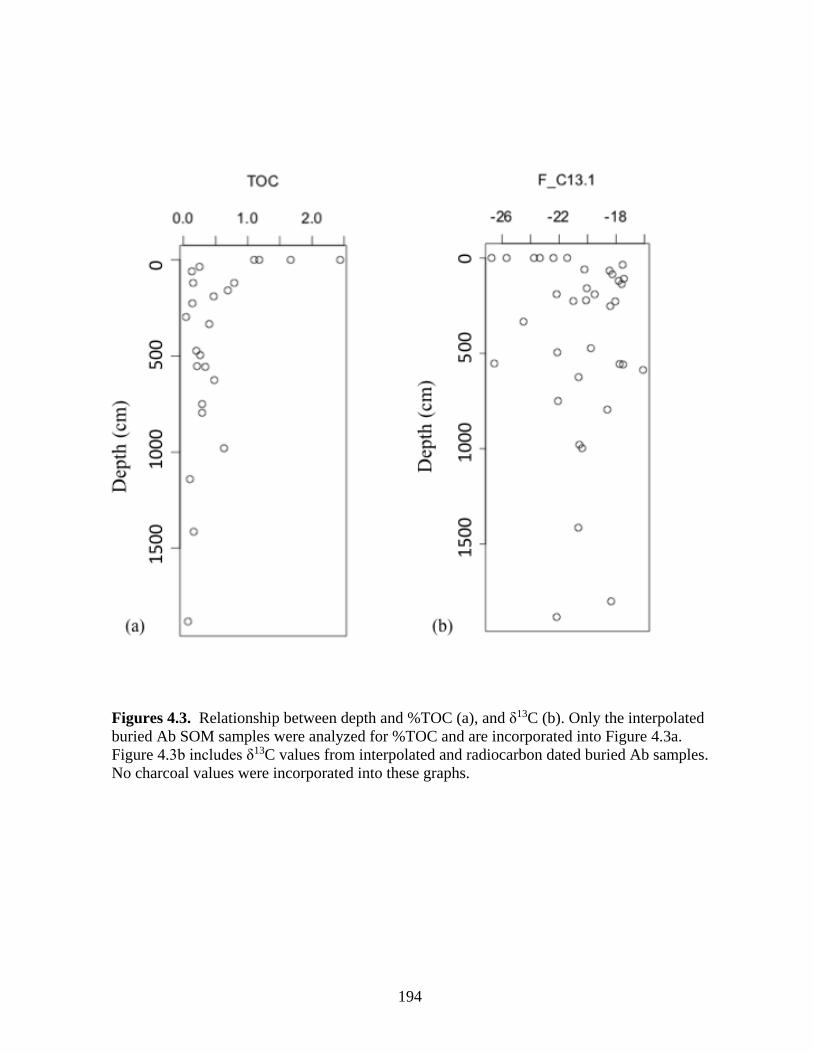
194
Figures 4.3. Relationship between depth and %TOC (a), and δ13C (b). Only the interpolated
buried Ab SOM samples were analyzed for %TOC and are incorporated into Figure 4.3a.
Figure 4.3b includes δ13C values from interpolated and radiocarbon dated buried Ab samples.
No charcoal values were incorporated into these graphs.

195
Figure 4.4. Distribution of δ13C values from the Culebra, Verde and Inguiro watersheds
(not including the charcoal sample values) including the mean (black horizontal line), the
standard deviation (box), and the individual δ13C values (black dots) for different time
periods. The modern values reflect the +1.5‰ related to the Suess effect.
δ1
3C
(‰
)
Late Holocene Middle Holocene Terminal Pleistocene-
early Holocene
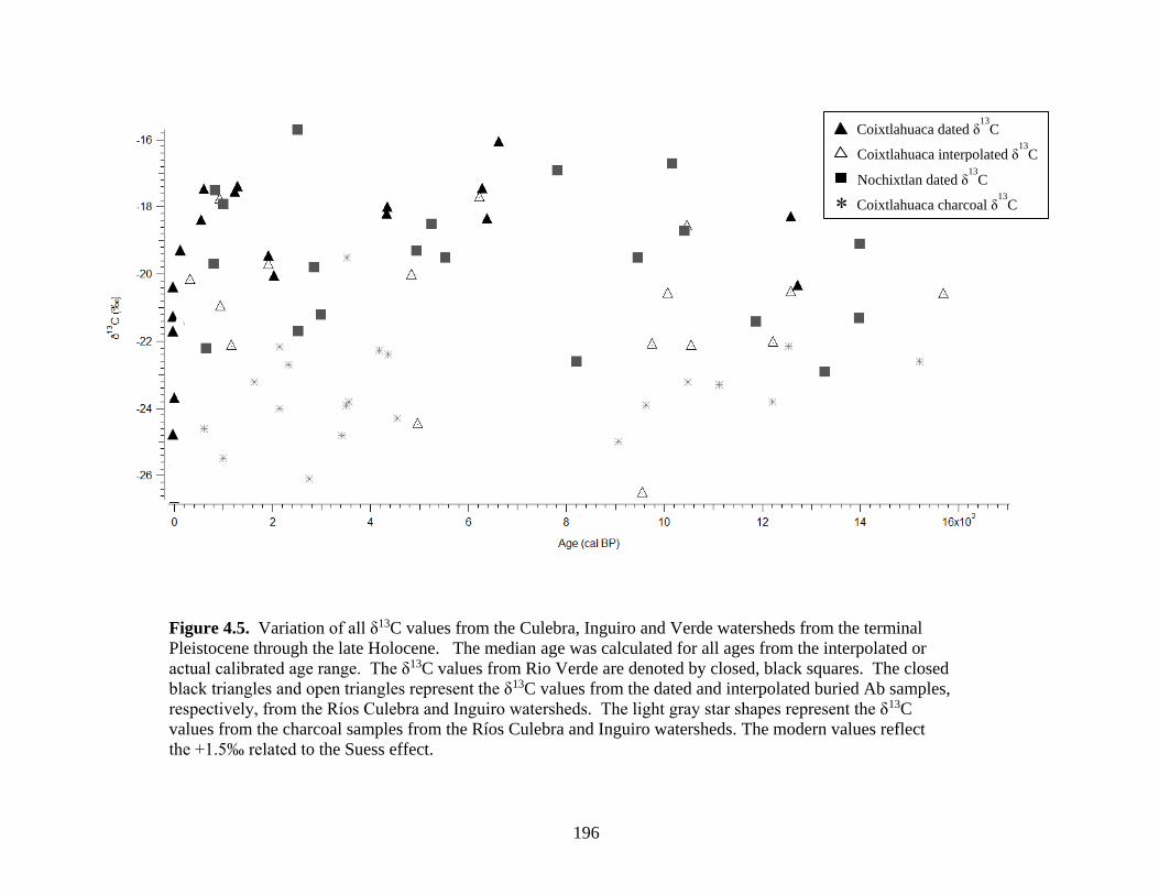
196
Figure 4.5. Variation of all δ13C values from the Culebra, Inguiro and Verde watersheds from the terminal
Pleistocene through the late Holocene. The median age was calculated for all ages from the interpolated or
actual calibrated age range. The δ13C values from Rio Verde are denoted by closed, black squares. The closed
black triangles and open triangles represent the δ13C values from the dated and interpolated buried Ab samples,
respectively, from the Ríos Culebra and Inguiro watersheds. The light gray star shapes represent the δ13C
values from the charcoal samples from the Ríos Culebra and Inguiro watersheds. The modern values reflect
the +1.5‰ related to the Suess effect.
*
Coixtlahuaca dated δ13
C
Coixtlahuaca interpolated δ13
C
Coixtlahuaca charcoal δ13
C
Nochixtlan dated δ13
C

197
Figures 4.6. Local polynomial regression indicating the main trend of all δ13C
values over time. Graph 4.6a excludes the outliers, while graph 4.6b excludes both
outliers and the interpolated δ13C values. Neither of the graphs include the δ13C
values from the charcoal samples. Note two peaks in the data, the first of which is
in the middle Holocene and the second is in the late Holocene, between ~1,250-500
cal BP. The analysis was made in R statistical software (R core team) using the
LOESS function (Cleveland et al 1992). The modern values are averaged and
reflect the +1.5‰ related to the Suess effect.
(b)
(a)
δ1
3C
(‰
)
Age (Cal BP)

198
Figure 4.7. Summary of the climatic data in central and southwestern Mexico for the last 16,000 years.
Age (Cal BP)
199
Note: Caption refers to figure on previous page.
Figure 4.7. Summary of the climate data in central and southwestern Mexico for the last 16,000
years. This information is organized by region (listed on right) and type of proxy data (listed on
left) for the upper portion (top 1/4th) of the figure. Below this regional organization is
information concerning glaciers from central Mexico, %C4 and CAM and paleosol information
from the study area and the Río Verde basin. The second portion of the graph shows the δ18O
signature from stalagmites in Guerrero, Mexico and CO2 information.
Information for figure and in text is summarized from the following articles: 1) Puebla-Tlaxcala (Metcalfe et al.,
2000); 2) Basin of Mexico (from Metcalfe et al., 2000; Lozano-Garcia and Ortega-Guerrero, 1998; Lozano-Garcia
and Vazquez-Selem) 3) Upper Lerma (Metcalfe et al., 2000; Lozano-Garcia et al., 2005; ) ; 4) Lake Patzcuaro,
Lake Zirahuen, Lake Zacapu (Metcalfe et al., 2000; Bradbury, 1989; Bradbury, 2000; Lozano-Garcia et al., 2013);
5) Guanajato and Michoacán (Metcalfe et al., 2000; Park et al., 2010); 6) Glaciers: (Metcalfe et al., 2000; Lozano-
Garcia and Vazquez-Selem, 2005; Vazquez-Selem and Heine, 2011); 7) %C4/CAM (this study, Rio Verde
information from Mueller et al., 2012); 8) paleosol information (Mueller et al., 2012; Chapter 3); 9) δ18O from
Guerreran stalagmites (Bernal et a., 2011; Lachniet et al., 2013); 10) past atmospheric CO2 from the Antarctic ice
cores (Monnin et al 2001; 2004); lake carbonate isotope data (Lozano-Garcia et al., 2010); 11) δ13C data (this
study, includes data from Verde watershed, Mueller et al., 2012); 12) archaeological time periods (Kowalewski et
al., 2009, Kowalewski, pers. com).

200
Figure 4.8. Z-score calculations for selected paleoclimatic datasets.
(a)
(b)
(c)
(d)
(e)
(f)
(g)
(h)
201
Note: Caption refers to figure on previous page.
Figure 4.8. Z-score calculations for selected paleoclimatic datasets. Information for figure and in text is summarized from
the following studies: (a) %Al2O3 from Cuenca Oriental (Bhattacharya et al. 2015); (b) % Sand from El Junco Basin
(Conroy et al., 2008); (c) %Ti from Cariaco Basin (Haug et al., 2001); (d) δ18O (‰)from Guerreran stalagmites (Bernal et
a., 2011; Lachniet et al., 2013); (e) δ18O (‰) from Cuenca Oriental (Bhattacharya et al. 2015); (f) δ13C (‰) from Cuenca
Oriental (Bhattacharya et al. 2015); (g) (d) δ13C (‰) from the Cueva del Diablo (Guerrero) (Bernal et a., 2011); and (h)
δ13C data (this study, includes data from Verde watershed, Mueller et al., 2012).

202
Site Depth (cm) Calibrated Age
(2-sig) Median
δ13C
values
Analysis 11
δ13C
values
Analysis 2
Paleosol
δ13C values
from C14
dating
Charcoa
l δ13C
values
Final
δ13C2
Total
Organic
Carbon3
Apo Forest NA MODERN -26.73 NA NA NA -25.23 1.1
Ast Grassland NA MODERN -22.39 NA NA NA -20.89 1.67
Vic
Mixed
grass/
succulent
NA MODERN -23.34 NA NA NA -21.84 2.44
Vic
Mixed
grass/forest/
succulent
NA MODERN -25.68 NA NA NA -24.18 1.18
C1 395 2060-2300c NA NA NA NA -23.6 -23.6 NA
C1 800 12421-12619c NA NA NA NA -23.7 -23.7 NA
Table 4.1. Results of the δ13
C values analyses. The results include analyses made on dated and
interpolated buried A SOM samples, as well as from charcoal samples from the Culebra and Inguiro
watersheds. The ages from the dated buried A SOM and charcoal samples were calibrated using the
online CALIB software (Stuiver et al., 2015) and the INTCAL2013 calibration curve (Riemer et al.,
2013). The ages of the interpolated buried A SOM samples were estimated using the Classical Age Model
(CLAM) of Blaauw (2010, version 2.2) with R software (R Core Team, 2013).

203
C1 300 NA NA -22.27 NA NA NA -22.27 0.13
C1 950 NA NA -22.14 NA NA NA -22.14 0.4
C2 190 1073-1251* 1162 -22.17 NA NA NA -22.17 0.47
C2 222 1949-2114 2028 NA NA -20.1 NA -20.1 NA
C2 334 4898-5019* 4959 -24.49 NA NA NA -24.49 0.4
C2 490 89999-9133c NA NA NA -25 -25
C2 553 9468-9640* 9554 (-30.17˨) -22.91 NA NA -22.91 0.35
C2 979 12550-12611* 12581 NA -20.57 NA NA -20.57 0.63
C2 997 12684-12750 12717 NA NA -20.38 NA -20.38
C2 1414 15589-15798* 15694 -20.28 -21 NA NA -20.64 0.16
C2 1882 18828-19218* 10553 (-20.18˨) -22.17 NA NA -22.17 0.07
I10
Mixed
grassland/
succulent
*** MODERN NA NA -21.42 NA -19.92 NA
I10 36 NA NA -20.92 -19.29 NA NA -20.11 0.25
I10 226 881-998* 940 -20.58 -21.4 NA NA -20.99 0.14
I10 243 939-1057c NA NA NA NA -25.49 -25.49 NA
I10 473 1855-1987* 1921 -20.21 -19.98 -19.42 NA -19.76 0.2
I10 802 4039-4281c NA NA NA NA -22.26 -22.26 NA
S11 120 NA NA (-19.41˨) -20.95 NA NA -20.95 0.15
S4
Mixed
grassland/
succulent
*** MODERN NA NA -23.75 NA -22.25 NA
S4 60 286-349* 318 -20.1 NA NA NA -20.21 0.13

204
S4 105 531-641c NA NA NA NA -24.6 -24.6 NA
S4 120 881-978* 930 -17.81 NA NA NA -17.81 0.79
S4 398 4256-4425c NA NA NA NA -22.4 -22.4 NA
S4 517 4439-4784c NA NA NA NA -24.3 -24.3 NA
S4 556 6173-6274* 6224 (-28.744) -17.99 -17.5 NA -17.75 0.34
S4 559 6212-6307 6282 NA NA -17.5 NA -17.5 NA
S4 587 6507-6674 6620 NA NA -16.1 NA -16.1 NA
S4 712 11808-11201c NA NA NA NA -23.3 -23.3 NA
S4 750 11986-12444* 12215 -21.24 -22.89 NA NA -22.07 0.29
S4 1140 24852-26488* 25670 -21.06 -22.04 NA NA -21.55 0.1
S5 280 1562-1698c NA NA NA NA -23.2 -23.2 NA
S5 67 518-629 544 NA NA -18.45 NA -18.45 NA
S5 191 1873-1988 1919 NA NA -19.5 NA -19.5 NA
S5 434 2721-2760c NA NA NA NA -26.1 -26.1 NA
S5 1081 3377-3479c NA NA NA NA -24.8 -24.8 NA
S6 109 1266-1309 1291 NA NA -17.44 NA -17.44 NA
S6 228 4249-4419 4348 NA NA -18.05 NA -18.05 NA
S7 137 1181-1278 1233 NA NA -17.6 NA -17.6 NA
S7 330 2048-2303c NA NA NA NA -24 -24 NA
S7 350 2184-2351c NA NA NA NA -22.7 -22.7 NA
S7 522 3453-3565c NA NA NA NA -23.9 -23.9 NA
S7 585 3480-3639c NA NA NA NA -23.8 -23.8 NA
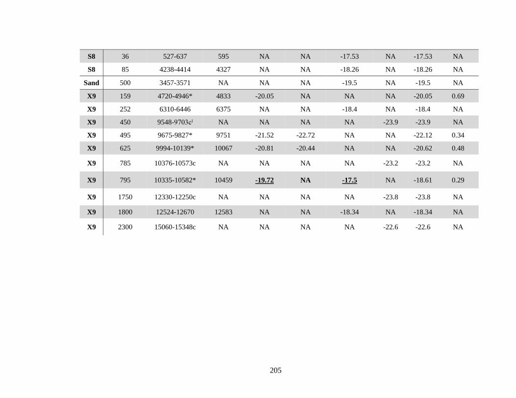
205
S8 36 527-637 595 NA NA -17.53 NA -17.53 NA
S8 85 4238-4414 4327 NA NA -18.26 NA -18.26 NA
Sand 500 3457-3571 NA NA NA -19.5 NA -19.5 NA
X9 159 4720-4946* 4833 -20.05 NA NA NA -20.05 0.69
X9 252 6310-6446 6375 NA NA -18.4 NA -18.4 NA
X9 450 9548-9703cˡ NA NA NA NA -23.9 -23.9 NA
X9 495 9675-9827* 9751 -21.52 -22.72 NA NA -22.12 0.34
X9 625 9994-10139* 10067 -20.81 -20.44 NA NA -20.62 0.48
X9 785 10376-10573c NA NA NA NA -23.2 -23.2 NA
X9 795 10335-10582* 10459 -19.72 NA -17.5 NA -18.61 0.29
X9 1750 12330-12250c NA NA NA NA -23.8 -23.8 NA
X9 1800 12524-12670 12583 NA NA -18.34 NA -18.34 NA
X9 2300 15060-15348c NA NA NA NA -22.6 -22.6 NA

206
Notes: 1The δ
13C values from the interpolated buried A SOM samples are presented in Analysis 1 and 2.
2If more than one δ
13C value was obtained for a corresponding profile and depth, they are averaged and presented
in the Final δ13
C column.3The percentage of the total organic carbon (%TOC) for the interpolated buried A SOM analyses are presented in
this column. These values represent an averaged value if the δ13
C values were averaged.
*δ13
C values with interpolated ages.
“c” = δ13
C values for charcoal ages.
“22.1” = δ13
C values from dated buried A SOM that were re-analyzed to determine their duplicability.4 δ
13C values removed from further analysis.
*** δ13
C values from surface A SOM that were dated to estimate soil residence time.
Table 4.2. The resulting modern δ13
C values after applying correction for the Suess effect. The
italized values represent the final accepted values.
Site Name Vegetation type Raw δ13C Final δ13C
(+1.5‰)
δ13C
(+2.0‰)
Apo Forest -26.73 -25.23 -24.73
Ast Grassland -22.39 -20.89 -20.39
S4 Mixed
grassland/succulent -23.75 -22.25 -21.75
Vic1 Mixed grass/succulent -23.34 -21.84 -21.34
Vic2 Mixed grass/forest/
succulent -25.68 -24.18 -23.68
I10 mixedMixed
grassland/succulent -21.42 -19.92 -19.42
Table 4.3. The modern δ13
C values used in calculating %C4 and CAM. The italized values
represent the final accepted values.
Vegetation Type δ13C Value (+1.5‰) (+2.0‰)
C3 wild -28 -26.5 -26
C3 cultivated -27.3
C4 wild -13.3 -11.8 -11.3
C4 cultivated -12
CAM wild 14.3
CAM cultivated 13.1
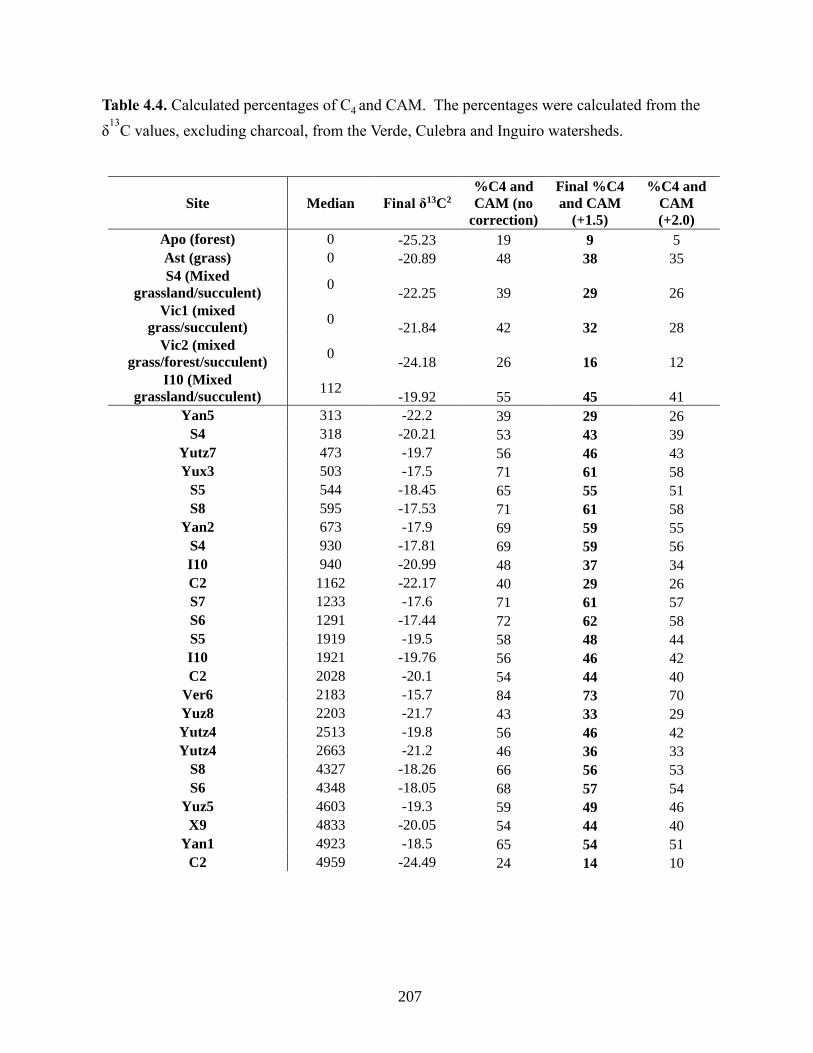
207
Table 4.4. Calculated percentages of C4 and CAM. The percentages were calculated from the
δ13
C values, excluding charcoal, from the Verde, Culebra and Inguiro watersheds.
Site Median Final δ13C2
%C4 and
CAM (no
correction)
Final %C4
and CAM
(+1.5)
%C4 and
CAM
(+2.0)
Apo (forest) 0 -25.23 19 9 5
Ast (grass) 0 -20.89 48 38 35
S4 (Mixed
grassland/succulent) 0
-22.25 39 29 26
Vic1 (mixed
grass/succulent) 0
-21.84 42 32 28
Vic2 (mixed
grass/forest/succulent) 0
-24.18 26 16 12
I10 (Mixed
grassland/succulent) 112
-19.92 55 45 41
Yan5 313 -22.2 39 29 26
S4 318 -20.21 53 43 39
Yutz7 473 -19.7 56 46 43
Yux3 503 -17.5 71 61 58
S5 544 -18.45 65 55 51
S8 595 -17.53 71 61 58
Yan2 673 -17.9 69 59 55
S4 930 -17.81 69 59 56
I10 940 -20.99 48 37 34
C2 1162 -22.17 40 29 26
S7 1233 -17.6 71 61 57
S6 1291 -17.44 72 62 58
S5 1919 -19.5 58 48 44
I10 1921 -19.76 56 46 42
C2 2028 -20.1 54 44 40
Ver6 2183 -15.7 84 73 70
Yuz8 2203 -21.7 43 33 29
Yutz4 2513 -19.8 56 46 42
Yutz4 2663 -21.2 46 36 33
S8 4327 -18.26 66 56 53
S6 4348 -18.05 68 57 54
Yuz5 4603 -19.3 59 49 46
X9 4833 -20.05 54 44 40
Yan1 4923 -18.5 65 54 51
C2 4959 -24.49 24 14 10

208
Yutz4 5193 -19.5 58 48 44
S4 6224 -17.75 70 60 56
S4 6282 -17.5 71 61 58
X9 6375 -18.4 65 55 52
S4 6620 -16.1 81 71 67
Yuz5 7483 -16.9 76 65 62
Yuz9 7873 -22.6 37 27 23
Yutz7 9123 -19.5 58 48 44
C2 9554 -22.91 35 24 21
X9 9751 -22.12 40 30 26
Yan4 9833 -16.7 77 67 63
X9 10067 -20.62 50 40 37
Yan2 10083 -18.7 63 53 50
X9 10458 -18.61 64 54 50
C2 10553 -22.17 40 29 26
Yan8 11543 -21.4 45 35 31
S4 12215 -22.07 40 30 27
C2 12581 -20.57 51 40 37
X9 12583 -18.34 66 56 52
C2 12717 -20.38 52 42 38
Yuz9 12943 -22.9 35 24 21
Yuz12 13643 -21.3 46 35 32
Yutz4 13663 -19.1 61 50 47
C2 15694 -20.64 50 40 36
S4 25670 -21.55 44 34 30

209
CHAPTER 5
CONCLUSION
5.1 Introduction
The incomplete understanding of present and past climatic change and the variability of
hydrological response to climate and land use change in dryland tropical regions is cause for
great concern. The problems of dryland regions in Mexico are no exceptions, with only a few
investigations into the nature and causes of erosion in dryland stream systems (Julio Falfan of
ConAgua, pers. Com., Rafael Arzate Aguirre of the Reserva de la Biosfera, pers. Com., and as
stated in Butzer et al., 2008; Mueller et al., 2012). The state of Oaxaca is home to many
indigenous populations, whose livelihoods depend on their local environment. The highly
degraded landscape of the Mixteca Alta embodies the dilemma of dryland desertification.
Oaxaca is in one of the two poorest states in Mexico, and many people partially rely on
government aid and intervention. The Mixteca Alta is one of the poorest areas in Oaxaca, not
only in terms of financial needs, but also in relation to its impoverished environment. Foraging
and managing of local plants, cultivating, and animal herding provide sustenance and
supplementary income to the rural population of this region. Several national organizations,
including the National Park Service, have worked with local communities to implement
governmentally subsidized conservation measures. However, without more information on the

210
various causes of degradation and the variability of local dryland stream systems, it is difficult
to assess the short and long-term effectiveness of these solutions on a basin-wide scale.
Examination of the late Quaternary environment and geomorphology of the incised,
ephemeral tributaries forming the Río Culebra watershed offered insight about causes of erosion
and hydrological variability of the region. This integrated study confirmed the variable and
intricate nature of semi-arid dryland fluvial systems. Climate change, land use factors, and
innate watershed characteristics (e.g., influential natural factors) have an integrated role in
producing erosion and modifying stream response during the late Holocene. Despite present
conservation efforts, climate change, present land use, and legacy effects from prehistoric and
Colonial land use all impede a straightforward solution to restoring the landscape on a basin
wide scale.
The arroyos of the Río Culebra watershed, and much of the Mixteca Alta, are
particularly complex as they involve both perennial and ephemeral streams, all of which incise
and aggrade on a cyclical timescale (Bull, 1997; Graf, 2002). As such, no stepped terraces are
observed in the valley, meaning more than 15,000 years of alluvial deposits reflecting
hydrologic responses to external drivers are entangled in the valley alluvium. Although the
Culebra watershed only covers 82 km2, the findings shed light onto better understanding the
desertification problem in the entire Mixteca Alta, and other drylands worldwide.
5.2 Climate and Hydrology: Long-Term Variability
The earliest date of cut-and-fill stratigraphy at ~15,000 cal BP demonstrates that at least
since the terminal Pleistocene, arroyo cycles have been a significant feature of the
211
geomorphology of the Mixteca Alta. The easily erodible geology of the Yanhuitlan beds in the
Mixteca Alta makes these areas extremely vulnerable to any climatic and land use changes (as
in McAuliffe and McFadden, 1997).
The semi-arid climate of the Mixteca Alta results from the rain shadow effect of the high
Mexican orography, in particular the Sierra Madre del Sur. Precipitation in the region is
variable and intensity is high. The current rainy season is attributed to the timing and strength of
the North American Monsoon, which are affected by both la Niña and El Niño phases of El
Niño Southern Oscillation (Vera et al., 2006).
The ephemeral tributary arroyos of the Río Culebra have many traits in common with
other sand-gravel dominated headwater dryland streams including rectangular channel form,
lack of armouring, subtle bedforms, and variable but intense scour-and-fill (Hassan et al., 2009;
Billi, 2011; Lucia et al., 2016). The channel morphology comprises a single-threaded main
channel that has some braiding with bars and minor channels. Minimum bedload yield of 17
and 45 t day-1 measured during individual runoff events from Barrancas Sandage and Sauce,
respectively, indicate that the watershed has high bedload yield typical of other semi-arid
environments. Floods in the Culebra watershed are extremely flashy and highly concentrated,
though they are often relatively shallow. High bedload yield and shallow floods in conjunction
with the various traits expressed above support high bedload flux under relatively low shear
stress and equal mobility of particles as observed in other ephemeral streams (e.g., Reid et al.,
1996; Lucia et al., 2016). Examining the alluvium-paleosol chronology of the Culebra, Inguiro,
and Verde (Mueller et al., 2012) watersheds against the high-resolution δ18O signature from
Guerreran stalagmites (Bernal et al., 2011; Lachniet et al., 2013) suggested that incision occured
212
during wetter periods, which corresponds to findings in other studies (Harden et al., 2010). This
comparison also suggested that alluvial deposition and paleosol formation occurred during
transitional wet and dry periods, which correspond to relatively drier periods than those
associated with incision and offers support for the “wet-dry-wet” model of arroyo cycles
(Waters and Haynes, 2001; Hereford, 2002; Huckleberry and Duff, 2008, Harden et al., 2010).
Overarching paleosol characteristics since the latest Pleistocene support the idea that wet and
dry fluctuations are an important component of the climate, and in general, support the idea that
alluvium/paleosol deposition/formation was prevalent during relatively drier, transitional wet
and dry periods. The importance of dry conditions in the area is demonstrated by the
widespread Stage I CaCO3 deposited on ped faces and in root pores in most horizons
(Birkeland, 1984).
The δ13C values obtained from buried soil organic matter exhibit a non-random
distribution through time and reflect overarching climate change from the terminal Pleistocene
to the early Holocene. When compared to various climatic proxies for central Mexico (e.g.,
Lozano-Garica and Ortega-Guerrero, 1998; Metcalfe et al., 2000), as well as to the δ18O from
stalagmites in southwestern Mexico (Bernal et al., 2011; Lachniet et al; 2013), the calculated
percentages of %C4 and CAM reflected both temperature and moisture fluctuations. The
transition of low to moderate percentages of C4 and CAM biomass in the terminal Pleistocene
and early Holocene toward high percentages in the middle Holocene signals the transition from
cool and dry towards warm and dry conditions. The late Holocene stable carbon isotope values
were varied and confounded by land use changes.
213
The variability and polygenetic nature of many paleosols limited their use to reconstruct
past climatic and environmental conditions, though they did provide some insight about past
conditions. Paleosols offered useful information on the paleohydrology associated with arroyo
cycles (as in Aslan and Autin, 1998). Unweathered alluvium and paleosol formation in
alluvium are two end members of alluvial stratigraphy. Paleosols represent relatively stable
surfaces that may be local or widespread, where and/or when aggradation slows or ceases. The
value of alluvial paleosols is how they fit into the range of alluvial deposits, how the variations
in the stratigraphy reflect paleohydrology, and how this provides information about prevailing
environmental conditions. For example, cumulic A horizons form on floodplains when
aggradation is slow enough to allow for pedogenesis. Cumulic A horizons were observed in
both the Culebra and Verde watersheds from the late Pleistocene to the late Holocene, but not
noted in the present-day arroyos, suggesting the prehistoric cumulic A horizons form in less
flashy conditions than that presently.
Observations from present bedload yield, flow characteristics, channel bed morphology,
and stratigraphy offered further insight on interpreting and understanding the Quaternary
alluvial stratigraphy (as in Reid, 2002; Billi, 2008). The nature of sediment characteristics of
flows and bedload yield in present-day systems suggested that similar traits observed in
stratigraphy reflect similar flood regimes in the past. For example, massive, coarse sandy to
fine gravel matrix-supported deposits in some alluvial strata resemble the deposits of present
flash floods. Overall finer deposits, with clear laminations and thin beds are observed in present
patchy floodplain deposits, contrasting with the prevalence of even finer deposits in the alluvial

214
stratigraphy. The overall finer deposits support more extensive floodplain construction during
aggradation phases.
5.3 Anthropogenic Drivers
Past and present land use has impacted sedimentation rates, sediment supply, vegetation
cover and type, and channel form. The Cruz phase (3,500 cal BP to 2,000 cal BP) agricultural
constructions were observed from the headwaters to the basin outlet in Barranca Sandage (~4
km2) (Leigh et al., 2013), and according to an archaeological survey they were continuously
used through the Natividad phase, despite population fluctuations (Kowlewski et al., 2009). In
contrast to the Cruz phase, lama-bordos and terrace walls were observed throughout much of
the Culebra watershed in the Natividad phase, which has an area of 82 km2. Sedimentation
rates behind lama-bordo walls during the late Holocene were more than two times higher than
that in the earlier Holocene and terminal Pleistocene, demonstrating the effectiveness of lama-
bordos as sediment traps. However, it appears that sedimentation rates were not affected on a
widespread scale until the Natividad phase.
Vegetation type, and the present scarcity of vegetation cover, has resulted from natural
and cultural factors. The region’s present biodiversity, including endemic succulent plants,
forestland, grasses, and woody vegetation, is a product of climate change, as well as prehistoric
and recent land use. Prehistoric impact on local vegetation is reflected in the δ13C values from
buried A soil organic matter, showing a significant rise from ~3,500 cal BP until between
1,000-500 cal BP. The increasingly enriched δ13C values in the late Holocene suggest that
intensified maize agriculture and possibly the increased management of succulent plants were

215
becoming very important to the ecological and cultural adaptation of the Mixteca Alta, and that
by the Natividad phase these species dominated parts of the landscape. It is unclear to what
extent deforestation took place in the past. Present agricultural land is not well managed and
vulnerable to erosion, and deforestation has resulted in much soil loss and reduction in biomass.
Various activities such as pumping water downstream and modern constructions on the Culebra
and its tributaries including fords, bridges, and check dams have all resulted in internal channel
adjustments including the formation of knickpoints.
5.4 Epilogue
Comparing the alluvium-paleosol stratigraphy to regional climatic change aided in
connecting paleohydrology to climatic drivers before intensive land use, but there were still
issues of equifinality. The comparison was complicated by the fact that the beginning of
agriculture in the region overlapped with the transition from the influence of the North Atlantic
on the spatio-temporal variability of the North American Monsoon to ENSO as the dominant
influence (Bernal et al., 2011). During the late Holocene, climate appears to have been the
dominant driver until the Natividad phase. Prior to the Natividad phase, land use activities
interacted with climate to produce hydrologic changes at a local scale, whereas during and after
the Natividad phase, widespread land use interacted with climate to affect changes on the
watershed scale. The subsequent abandonment of the lama-bordo system may have affected the
timing and nature (i.e., threshold-crossing event) of the most recent incision event around 1650
AD (Leigh et al., 2013), but did not cause the incision per se. Instead, prehistoric land use
altered sedimentation rates and storage in the landscape, as well as vegetation type and cover,

216
and the arrival of the Spanish resulted in further land use change, all of which interacted with
climate (e.g., precipitation amount and/or intensity) resulting in incision (Perroy et al., 2012).
For the past 15,000 years arroyo cycles have occurred as a result of external climatic
drivers compounded by local internal conditions. It is only during the late Holocene that
arroyos are influenced by human activities, and despite the new variable they persisted.
The present system of Río Culebra appears to be in complex response (as in Schumm, 1979),
adjusting to the long-term and short-term influences of late Holocene climate variation, legacies
of prehistoric land-use change, and modern land use. A forum on erosion and conservation in
the Mixteca Alta brought together local communities and local and national governmental
agencies including the National Park Service and Forest Service. From the presentations and
discussions in this forum, it was clear that local community leaders realize the need to preserve
and manage their environment and that unsustainable land use activities and climate change
cause land degradation. The Mexican government provides subsidies to reduce degradation and
implement conservation measures, however much of it depends on local labor, and available
funding is limited.
Evaluations of conservation measures have produced varying results (e.g., Fox et al.,
2016). Despite the well-conserved headwaters in Barranca Sandage, sediment yield was still
relatively high, suggesting that basin-wide conservation is needed. Interestingly, prehistoric
farmers installed check dams and terraces on a basin-wide scale; on Barranca Sandage earlier
on, and along the Culebra during the Natividad phase. Even so, the high sedimentation rates
and build up of material appeared to have had long-term effects, which emphasizes the need to
consider conservation at various temporal and spatial scales in the future.

217
5.5 References
Arzate Aguirre, Rafael, (per. Com). Coordinator of Conservation for the Biosphere Reserve
Tehuacán-Cuicatlán, National Park Commission, Mexico.
Aslan, A., Autin, W.J., 1998. Holocene flood-plain soil formation in the southern lower
Mississippi Valley: Implications for interpreting alluvial paleosols. Geological Society
of America Bulletin 110, 433-449.
Bernal, J., Lachniet, M., McCulloh, M., Mortimer, G., Morales, P., Cienfuegos, E., 2011. A
Speleothem Record of Holocene Climate Variability from Southwestern Mexico.
Quaternary Research 75, 104-113.
Billi, P., 2008. Bedforms and sediment transport processes in the ephemeral streams of Kobo
basin, Northern Ethiopia. Catena 75, 5-17.
Billi, P., 2011. Flash flood sediment transport in a steep sand-bed ephemeral stream.
International Journal of Sediment Research 26, 193-209.
Birkeland, P.W., 1984. Soils and Geomorphology. Oxford University Press, New York.
Butzer, K.W., Abbott, J.T., Frederick, C.D., Lehman, P.H., Cordova, C.E., Oswald, J.F., 2008.
Soil-geomorphology and "wet" cycles in the Holocene record of North-Central Mexico.
Geomorphology 101, 237-277.
Bull, W.B., 1997. Discontinuous ephemeral streams. Geomorphology 19, 227-276.
Falfan, Julio of ConAgua (pers. Com.). Meterologist at the Nation Comission of Water in
Oaxaca.
Graf, W.L., 2002. Fluvial Processes in Dryland Rivers. The Blackburn Press, Caldwell.
Harden, T., Macklin, M.G., Baker, V.R., 2010. Holocene flood histories in south-western USA.
Earth Surface Processes and Landforms 35, 707-716.
Hassan, M.A., Marren, P.M., Schwartz, U., 2009. Bar structure in an arid ephemeral stream.
Sedimentary Geology 221, 57-70.
Hereford, R., 2002. Valley-fill alluviation during the Little Ice Age (ca. AD 1400-1880), Paria
River basin and southern Colorado Plateau, United States. Geological Society of
America Bulletin 114, 1550-1563.
218
Huckleberry, G., Duff, A.I., 2008. Alluvial cycles, climate, and puebloan settlement shifts near
Zuni Salt Lake, New Mexico, USA. Geoarchaeology-an International Journal 23, 107-
130.
Kowalewski, S.A., Balkansky, A. K., Walsh, L. R. S., Pluckhahn, T. J., Chamblee, J. F.,
Rodriguez, V. P., Espinosa, V. Y. H., Smith, C. A., 2009. Origins of the Nuu:
Archaeology in the Mixteca Alta, Mexico. University Press Colorado, Boulder.
Lachniet, M., Asmerom, Y., Bernal, J., Polyak, V., Vaquez-Selem, L., 2013. Orbital Pacing and
Ocean Circulation-Induced Collapses of the Mesoamerican Monsoon over the past
22,000 yr. Proc Natl. Acad. Sci. U.S.A. 110, 9255-9260.
Leigh, D.S., Kowalewski, S.A., Holdridge, G., 2013. 3400 years of agricultural engineering in
Mesoamerica: lama-bordos of the Mixteca Alta, Oaxaca, Mexico. Journal of
Archaeological Science 40, 4107-4111.
Lozano-Garcia, M.D., Ortega-Guerrero, B., 1998. Late Quaternary environmental changes of
the central part of the Basin of Mexico; Correlation between Texcoco and Chalco basins.
Review of Palaeobotany and Palynology 99, 77-93.
Lucia, A., Recking, A., Martin-Duque, J.F., Storz-Peretz, Y., Laronne, J.B., 2013. Continuous
monitoring of bedload discharge in a small, steep sandy channel. Journal of Hydrology
497, 37-50.
McFadden, L.D., McAuliffe, J.R., 1997. Lithologically influenced geomorphic responses to
Holocene climatic changes in the Southern Colorado Plateau, Arizona: A soil-
geomorphic and ecologic perspective. Geomorphology 19, 303-332.
Metcalfe, S.E., O'Hara, S.L., Caballero, M., Davies, S.J., 2000. Records of Late Pleistocene-
Holocene climatic change in Mexico - a review. Quaternary Science Reviews 19, 699-
721.
Mueller, R.G., Joyce, A.A., Borejsza, A., 2012. Alluvial archives of the Nochixtlan valley,
Oaxaca, Mexico: Age and significance for reconstructions of environmental change.
Palaeogeography Palaeoclimatology Palaeoecology 321, 121-136.
Perroy, R.L., Bookhagen, B., Chadwick, O.A., Howarth, J.T., 2012. Holocene and
Anthropocene Landscape Change: Arroyo Formation on Santa Cruz Island, California.
Annals of the Association of American Geographers 102, 1229-1250.
Poesen, J., Nachtergaele, J., Verstraeten, G., Valentin, C., 2003. Gully erosion and
environmental change: importance and research needs. Catena 50, 91-133.
219
Reid, I., Powell, D.M. and Laronne, J.B., 1996. Prediction of bed-load transport by desert flash
floods. Journal of Hydraulic Engineering-Asce, 122(3): 170-173.
Reid, I., 2002. Sediment Dynamics of Ephemeral Channels, in: Bull, L.J., Kirkby, M.J. (Eds.),
Dryland Rivers: Hydrology and Geomorphology of Semi-Arid Channels. John Wiley &
Sons Ltd., Wests Sussex.
Schumm, S.A., 1974. Geomorphic thresholds and complex response of drainage systems, in
Morisawa, M, ed., Fluvial Geomorphology. State University of New York at
Binghamton, Publications in Geomorphology, pp. 299-310.
Schumm, S.A., 2005. River Variability and Complexity. Cambridge University Press,
Cambridge.
Valentin, C., Poesen, J., Li, Y., 2005. Gully erosion: Impacts, factors and control. Catena 63,
132-153.
Vera, C., Higgins, W., Amador, J., Ambrizzi, T., Garreaud, R., Gochis, D., Gutzler, D.,
Lettenmaier, D., Marengo, J., Mechoso, C.R., Nogues-Paegle, J., Silva Dias, P.L.,
Zhang, C., 2006. Toward a unified view of the American Monsoon Systems. Journal of
Climate 19, 4977-5000.
Waters, M.R., Haynes, C.V., 2001. Late Quaternary arroyo formation and climate change in the
American Southwest. Geology 29, 399-402.
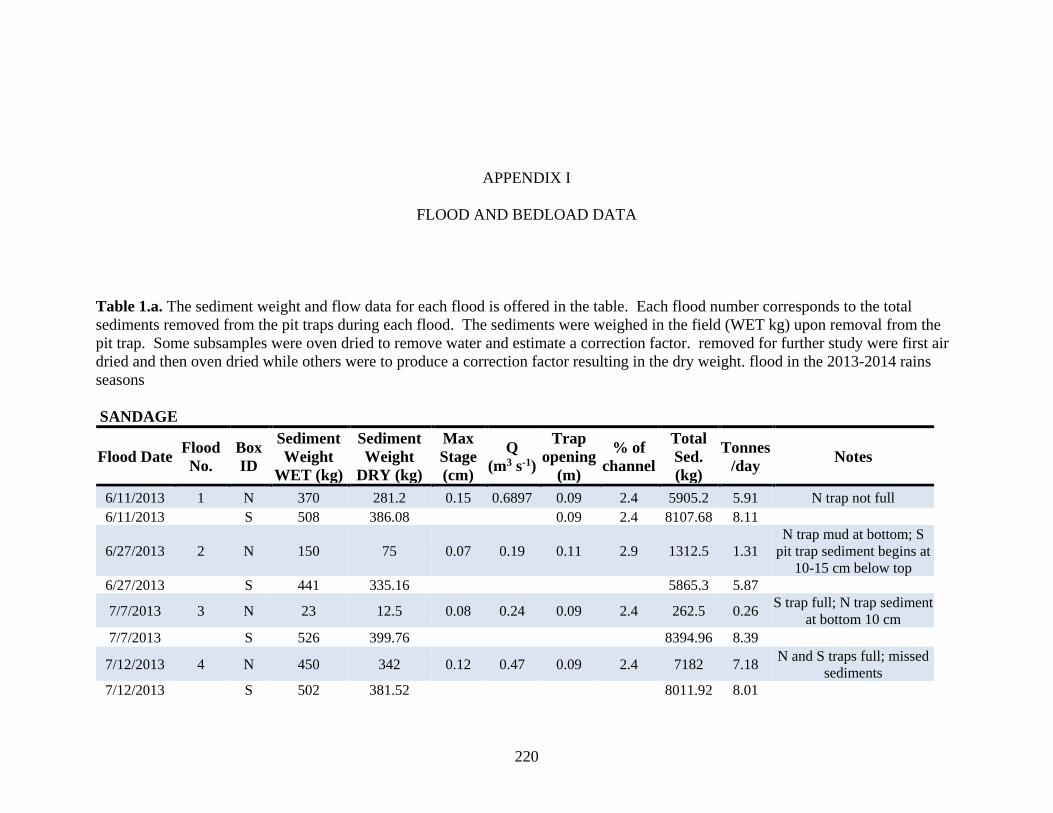
220
APPENDIX I
FLOOD AND BEDLOAD DATA
Table 1.a. The sediment weight and flow data for each flood is offered in the table. Each flood number corresponds to the total
sediments removed from the pit traps during each flood. The sediments were weighed in the field (WET kg) upon removal from the
pit trap. Some subsamples were oven dried to remove water and estimate a correction factor. removed for further study were first air
dried and then oven dried while others were to produce a correction factor resulting in the dry weight. flood in the 2013-2014 rains
seasons
SANDAGE
Flood Date Flood
No.
Box
ID
Sediment
Weight
WET (kg)
Sediment
Weight
DRY (kg)
Max
Stage
(cm)
Q
(m3 s-1)
Trap
opening
(m)
% of
channel
Total
Sed.
(kg)
Tonnes
/day Notes
6/11/2013 1 N 370 281.2 0.15 0.6897 0.09 2.4 5905.2 5.91 N trap not full
6/11/2013 S 508 386.08 0.09 2.4 8107.68 8.11
6/27/2013 2 N 150 75 0.07 0.19 0.11 2.9 1312.5 1.31
N trap mud at bottom; S
pit trap sediment begins at
10-15 cm below top
6/27/2013 S 441 335.16 5865.3 5.87
7/7/2013 3 N 23 12.5 0.08 0.24 0.09 2.4 262.5 0.26 S trap full; N trap sediment
at bottom 10 cm
7/7/2013 S 526 399.76 8394.96 8.39
7/12/2013 4 N 450 342 0.12 0.47 0.09 2.4 7182 7.18 N and S traps full; missed
sediments
7/12/2013 S 502 381.52 8011.92 8.01

221
7/21/2013 5 N 532 404.32 0.39 4.01 0.09 2.4 9501.52 9.50 N and S traps full; missed
sediments
7/21/2013 S 561 426.36 10019.46 10.02
9/2/2013 6 N 540 410.4 0.65 9.66 0.09 2.4 9849.6 9.85 N and S traps full; missed
sediments
9/2/2013 S 507 385.32 9247.68 9.25
9/26/2013 7 N 156 75.24 0.08 0.22 0.025 0.7 5718.24 5.72 S trap full; N trap
sediments at bottom 30 cm
9/26/2013 S 483 367.08 27898.08 27.90
10/1/2013 8 N 51 38.76 0.075 0.16 0.05 1.3 1472.88 1.47 S trap full; N trap
sediments at bottom 30 cm
10/1/2013 S 409 310.84 0.07 1.8 8392.68 8.39
6/18/2014 9 N 484 367.84 1.2 25.02 0.08 2.1 11035.2 11.04 N and S traps full; missed
sediments
6/18/2014 S 486 369.36 0.09 2.4 9603.36 9.60
6/24/2014 10 S 455 345.8 0.09 0.29 0.09 2.4 4841.2 4.84 N and S traps not full; M
trap full
6/24/2014 N 372 282.72 3958.08 3.96
6/24/2014 M 449 341.24 4777.36 4.78
7/4/2014 11 N 312 237.12 0.39 4.31 0.09 2.4 3793.92 3.79 N, S, and M traps full;
missed sediments
7/4/2014 S 473 359.48 5751.68 5.75
7/4/2014 M 442 335.92 5374.72 5.37
7/24/2014 12 N 454 345.04 0.36 3.76 0.09 2.4 5520.64 5.52 N, S, and M traps full;
missed sediments
7/24/2014 S 470 357.2 5715.2 5.72
7/24/2014 M 428 325.28 5204.48 5.20
8/10/2014 13 N 417 316.92 0.67 10.76 0.09 2.4 5387.64 5.39 N, S, and M traps full;
missed sediments
8/10/2014 S 434 329.84 0.09 2.4 5607.28 5.61
8/10/2014 M 442 335.92 0.05 1.1 10077.6 10.08
9/15/2014 14 N 363 275.88 0.15 0.68 0.09 2.4 3862.32 3.86 N, S, and M traps full;
missed sediments
9/15/2014 S 509 386.84 0.09 2.4 5415.76 5.42
9/15/2014 M 532 404.32 0.05 1.1 10108 10.12

222
Table 1.b. The sediment weight and flow data for each flood is offered in the table. Each flood number corresponds to the total
sediments removed from the pit traps during each flood. The sediments were weighed in the field (WET kg) upon removal from the
pit trap. Some subsamples were oven dried to remove water and estimate a correction factor. removed for further study were first air
dried and then oven dried while others were to produce a correction factor resulting in the dry weight. flood in the 2013-2014 rains
seasons
SAUCE
Flood Date Flood
No.
Box
ID
Sediment
Weight
WET (kg)
Sediment
Weight
DRY (kg)
Max
Stage
(cm)
Q
(m3 s-1)
Trap
opening
(m)
% of
channel
Total Sed.
(kg)
Tonnes
/day Notes
6/11/2013 1 1 526 399.76 0.51 20.46 0.05 0.5 16789.92 16.79
All traps full, missed
sediments
6/11/2013 2 521 395.96 0.51 20.46 0.05 0.5 16630.32 16.64
6/11/2013 3 526 399.76 0.51 20.46 0.05 0.5 16789.92 16.79
6/11/2013 4 540 410.4 0.51 20.46 0.05 0.5 17236.8 17.24
6/11/2013 5 533 405.08 0.51 20.46 0.05 0.5 17013.36 17.02
6/24/2013 2 1 526 399.76 0.035 0.19 0.11 1.1 7195.68 7.2
Traps 3, 4, and 5
almost full
6/24/2013 2 468 355.68 0.035 0.19 0.11 1.1 6402.24 6.41
6/24/2013 3 517 392.92 0.035 0.19 0.11 1.1 7072.56 7.08
6/24/2013 4 540 410.4 0.035 0.19 0.11 1.1 7387.2 7.39
6/24/2013 5 493 374.68 0.035 0.19 0.11 1.1 6744.24 6.75
7/12/2013 3 1 7 5.32 0.025 0.11 0.132 1.3 79.8 0.08
All traps contain only
mud and water
7/12/2013 2 4.5 3.42 0.025 0.11 0.11 1.1 61.56 0.07
7/12/2013 3 4.5 3.42 0.025 0.11 0.12 1.2 58.14 0.06
7/12/2013 4 7 5.32 0.025 0.11 0.12 1.2 90.44 0.1
7/12/2013 5 33 25.08 0.025 0.11 0.127 1.3 401.28 0.41
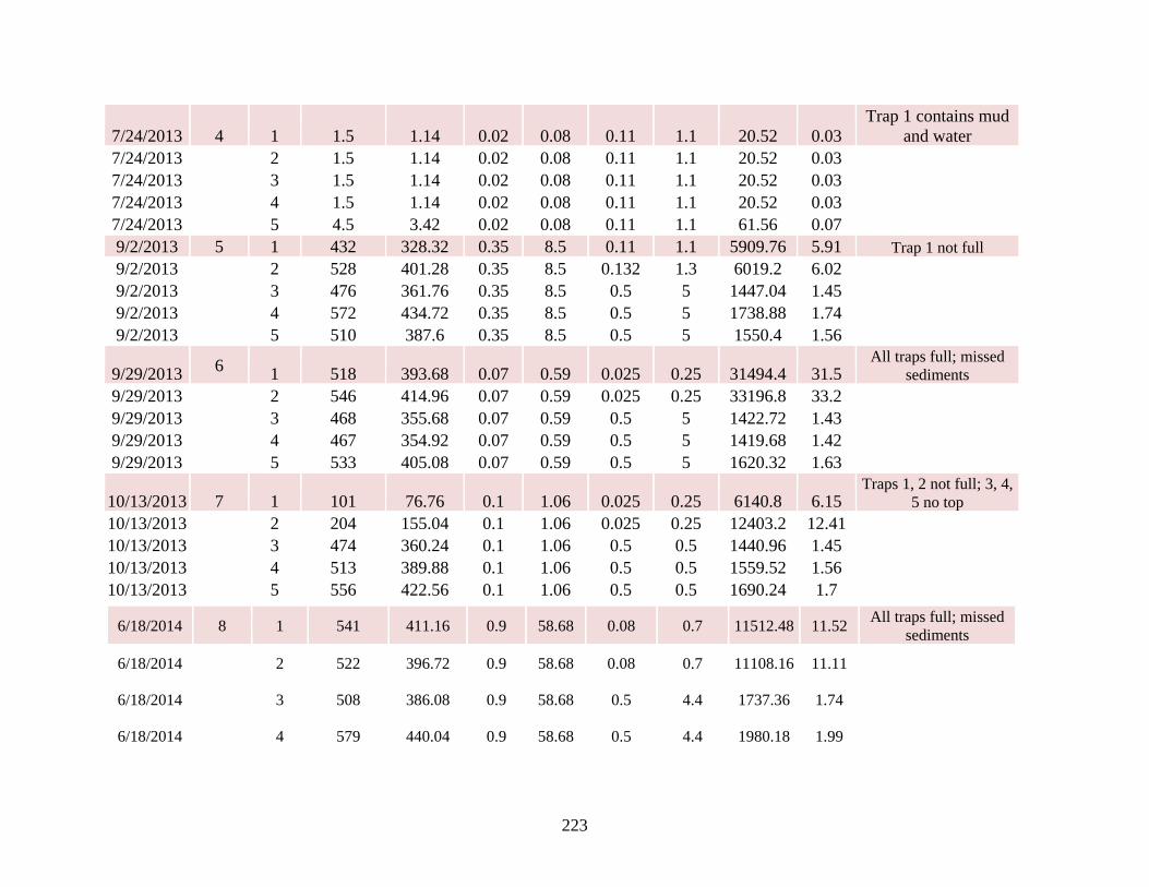
223
7/24/2013 4 1 1.5 1.14 0.02 0.08 0.11 1.1 20.52 0.03
Trap 1 contains mud
and water
7/24/2013 2 1.5 1.14 0.02 0.08 0.11 1.1 20.52 0.03
7/24/2013 3 1.5 1.14 0.02 0.08 0.11 1.1 20.52 0.03
7/24/2013 4 1.5 1.14 0.02 0.08 0.11 1.1 20.52 0.03
7/24/2013 5 4.5 3.42 0.02 0.08 0.11 1.1 61.56 0.07
9/2/2013 5 1 432 328.32 0.35 8.5 0.11 1.1 5909.76 5.91 Trap 1 not full
9/2/2013 2 528 401.28 0.35 8.5 0.132 1.3 6019.2 6.02
9/2/2013 3 476 361.76 0.35 8.5 0.5 5 1447.04 1.45
9/2/2013 4 572 434.72 0.35 8.5 0.5 5 1738.88 1.74
9/2/2013 5 510 387.6 0.35 8.5 0.5 5 1550.4 1.56
9/29/2013 6
1 518 393.68 0.07 0.59 0.025 0.25 31494.4 31.5 All traps full; missed
sediments
9/29/2013 2 546 414.96 0.07 0.59 0.025 0.25 33196.8 33.2
9/29/2013 3 468 355.68 0.07 0.59 0.5 5 1422.72 1.43
9/29/2013 4 467 354.92 0.07 0.59 0.5 5 1419.68 1.42
9/29/2013 5 533 405.08 0.07 0.59 0.5 5 1620.32 1.63
10/13/2013 7 1 101 76.76 0.1 1.06 0.025 0.25 6140.8 6.15 Traps 1, 2 not full; 3, 4,
5 no top
10/13/2013 2 204 155.04 0.1 1.06 0.025 0.25 12403.2 12.41
10/13/2013 3 474 360.24 0.1 1.06 0.5 0.5 1440.96 1.45
10/13/2013 4 513 389.88 0.1 1.06 0.5 0.5 1559.52 1.56
10/13/2013 5 556 422.56 0.1 1.06 0.5 0.5 1690.24 1.7
6/18/2014 8 1 541 411.16 0.9 58.68 0.08 0.7 11512.48 11.52 All traps full; missed
sediments
6/18/2014 2 522 396.72 0.9 58.68 0.08 0.7 11108.16 11.11
6/18/2014 3 508 386.08 0.9 58.68 0.5 4.4 1737.36 1.74
6/18/2014 4 579 440.04 0.9 58.68 0.5 4.4 1980.18 1.99

224
6/18/2014 5 552 419.52 0.9 58.68 0.5 4.4 1887.84 1.89
6/26/2014 9 1 424 322.24 0.05 0.33 0.08 0.8 8056 8.06 Trap 1, 2 almost full; 3,
4, 5 no top
6/26/2014 2 472 358.72 0.05 0.33 0.08 0.8 8968 8.97
6/27/2014 3 440 334.4 0.05 0.33 0.5 5 1337.6 1.34
6/26/2014 4 511 388.36 0.05 0.33 0.5 5 1553.44 1.56
6/27/2014 5 532 404.32 0.05 0.33 0.5 5 1617.28 1.62
7/9/2014 10 1 485 368.6 0.33 7.7 0.08 0.8 9215 9.22 All traps full; missed
sediments
7/9/2014 2 487 370.12 0.33 7.7 0.08 0.8 9253 9.26
7/9/2014 3 455 345.8 0.33 7.7 0.5 5 1383.2 1.39
7/9/2014 4 507 385.32 0.33 7.7 0.5 5 1541.28 1.55
7/9/2014 5 569 432.44 0.33 7.7 0.5 5 1729.76 1.73
7/24/2014 11 1 109 82.84 0.44 13.13 0.08 0.8 2071 2.08 Traps 1 almost full; 3,
4, 5 no top
7/24/2014 2 501 380.76 0.44 13.13 0.08 0.8 9519 9.52
7/24/2014 3 440 334.4 0.44 13.13 0.5 5 1337.6 1.34
7/24/2014 4 511 388.36 0.44 13.13 0.5 5 1553.44 1.56
7/24/2014 5 470 357.2 0.44 13.13 0.5 5 1428.8 1.43
8/10/2014 12 1 0 0 0.11 1.24 0.08 0.8 0 0 Trap 1 mud at bottom
8/10/2014 2 239 181.64 0.11 1.24 0.08 0.8 4541 4.55

225
8/10/2014 3 413 313.88 0.11 1.24 0.5 5 1255.52 1.26
8/10/2014 4 380 288.8 0.11 1.24 0.5 5 1155.2 1.16
8/10/2014 5 356 270.56 0.11 1.24 0.5 5 1082.24 1.09
9/21/2014 13 11 491 373.16 0.55 23.2 0.115 1.1 3358.44 3.36 All traps full; missed
sediments
9/21/2014 12 227 172.52 0.55 23.2 0.05 0.5 3622.92 3.63
9/21/2014 13 380 288.8 0.55 23.2 0.09 0.9 3465.6 3.47
9/21/2014 14 571 433.96 0.55 23.2 0.05 0.5 9113.16 9.12
9/21/2014 15 362 275.12 0.55 23.2 0.09 0.9 3301.44 3.31
9/21/2014 16 387 294.12 0.55 23.2 0.05 0.5 6176.52 6.18
9/21/2014 17 562 427.12 0.55 23.2 0.04 0.4 11105.12 11.11
9/21/2014 18 623 473.48 0.55 23.2 0.11 1 4734.8 4.74
9/21/2014 19 403 306.28 0.55 23.2 0.05 0.5 6431.88 6.44
9/21/2014 20 339 257.64 0.55 23.2 0.05 0.5 5410.44 5.42

226
APPENDIX II
PROFILE DESCRIPTIONS
Table II.a. The table shows the location information of the profiles.
Profile Name Site ID Site # Zone Easting Northing Barranca Field Notes
Sauce C1 SAU004 14Q 677603 1949394 Sauce Several cut and fills in headwater
tributaries of Río Culebra.
Confluence Site C2 435 47Q 322171 1958692 Culebra/Sandage/
Sandaxne
Well represented alluvium-
paleosol sequence at confluence
of tributary and midpart of the
main stem.
Río Culebra
Confluence C3 118 14Q 677933 1959690 Culebra
Well represent alluvium-paleosol
sequence on midpart of main
strem, Río Culebra.
Meander Bend I10 362 14Q 663885 1969963 Tributary to Inguiro
(JIcotlan)
Well represented alluvium-
paleosol sequence associated with
several lama-bordos.
Tusk-Horse S11 564 14Q 678419 1957101 Sandage
Cut-and-fill stratigraphy with part
of fossil mammoth tusk and other
Pleistocene horse jaw with several
teeth. Note highly oxidized C and
Bw horizon.
Magdalena
Culvert S4 122 14Q 678514 1957512 Sandage
Well represented alluvium-
paleosol sequence along
downstream part of tributary
arroyo Sandage.

227
Victor's Lama-
bordo S5 192 14Q 679457 1956286 Sandage
Well represented alluvium-
paleosol sequence associated with
very well-preserved ancient lama-
bordo in upper section of tributary
Sanage. Alluvial incision
associated with allostratigraphy
cuts into endeque and older (?)
paleosol.
Flores Amarillas S6 426 14Q 678905 1956480 Sandage
Well represented alluvium-
paleosol sequence on midstream
tributary of Sandage. Located
upstream from lama-bordo wall.
Thick, older paleosol also
observed in lower strata as in S5.
Island Site S7 68 14Q 678802 1956564 Sandage
Well represented paleosol-alluvial
sequence associated with (2?)
ancient lama-bordo(s) on tributary
of Sandage.
Juniper Site S8 424 14Q 678832 1956368 Sandage
Profile in first order tributary to
Sandage. Connects hillslope
sediments to valley.
Cliff Site X9 436 14Q 677926 1958596 Culebra/Sandage/Sandaxne
Well represented paleosol-alluvial
sequence at lower part of tributary
just before joins main stem;
includes lower cut and fill
Cuganda Sur / 514 14Q 677587 1959131 Inguiteria
Profile on shoulder near summit of
hillslope. Note paleosol beneath
endeque.
Sandaxne Site / 112 14Q 678421 1957945 Sandaxne
Allostraigraphy containing
mammoth bones and teeth in
massive deposits (colluvium?),
stratifraphically below a well-

228
defined paleosol, and above clear
fluvial deposits.
Inguirjo Site / 475 14Q 663822 1970732 Inguiro
Well represent paleosol-alluvial
sequence along mainstem of the
Río Inguiro, Jicotlan.
Two Coyote / Cul029 14Q 675527 1962009 Culebra
Cut-and-fill stratigraphy in the
downstream part of mainstem, Rio
Culebra. Some well-defined
paleosols noted.

229
Table II.b. Juniper Site Profile Description
Depth (cm) Horizon Color
(Dry) Texture Structure Boundary Remarks
C-14
Samples
0-12 C1 10YR 6/2 sil/mgr 3cogr clear much angular Yanhuitlan (moderate gravel)
12-30 C2 10YR 5.5/2 sil 2fgr clear less gravel than C1
30-42 Ab 10YR 5/2 sil 1mgr clear
few gravel clasts of mostly endeque (pottery
sherd) #201 bulk
42-55 C3 10YR 5/2 sil 1mgr clear less gravel than C1 (similar to C2)
55-67 Ab1' 10YR 5/1 sil 2fsbk clear few gravel Yanhuitlan (potsherd)
67-80 Ab2' 10YR 5/2 sil 2msbk clear
moderate amount of Yanhuiltan and endeque
gravel (potsherd)
80-90 2Ab3' 10YR 5/2 sicl 3msbk clear
tells him went from hillslope to Yanhuitlan
beds
#140;
#202 bulk
90-106 2AB 10YR 5/3 sicl 3cosbk gradual
abundant secondary CaCO3 nodules and root
filaments, uncertain whether nodules are
redeposited endeque or in situ ,
106-136 2Bt1bk 10YR 4/2 sicl 3cosbk clear
faint, thin, discontinuous, clay films on ped
faces. Abundant secondary CaCO3 nodules
and root filaments
136-170 2Bt2bk 10YR 6/4 sil 1fsbk gradual
few, thin, discontinuous clay films. CaCO3
as above but with larger nodules
170-190 2Ck 10YR 7/4 sil 1cosbk CaCO3 root filaments (no nodules)

230
Table II.c. Flores Amarillas Profile Description
Depth (cm) Horizon Color
(Dry) Texture Structure Boundary Remarks
C-14
Samples
(A section)
0-21 C cos sg A
21-64 Ab 10YR 4/3 sl 1fsbk C cumulic C14#244
64-71 C2 10YR 5/2 fgr-cos laminated G Endeque and Yanhuitlan clasts. Fining upward
sequences.
71-82 C3 10YR
4/2.5 sil 2msbk A Some root disturbance (krotovina). C14#243
82-104 2Ab 10YR 4/2 sil 1fsbk G Common Yanhuitlan and endeque clasts.
104-129 2Ab2 10YR 4/1 sil 2msbk C C14#160
129-170 2Ab3 10YR 4/1 sicl 3msbk G
170-221 C4 10YR 5/2 sil 2mpr C Common endeque nodules. Few Yanhuitlan
nodules. CaCO3 in root pores. C14#242
221-245 Ab' 10YR 3/2 sicl 3mpr A CaCO3 in root pores and ped faces. Few
Yanhuitlan clasts. C14#161
245-250 C5 10YR 6/2 sil m C fine-medium endeque gravel.
250-296 Ck6 10YR 6/2 sil 1fsbk D
Common endeque nodules. Common, distinct
CaCO3 in root pores. Few faint CaCO3 on ped
faces.
296-348 BC(k) -
AC? 10YR 5/1 sil 3msbk G
Common endeque nodules. Common, distinct
CaCO3 in root pores and on ped faces.
Yanhuitlan clasts.
348-368+ C7 10YR 6/2 sil 1vfsbk
Few, distinct CaCO3 in root pores and on ped
faces. Yanhuitlan and endeque clasts. (Much
less CaCO3 than above).
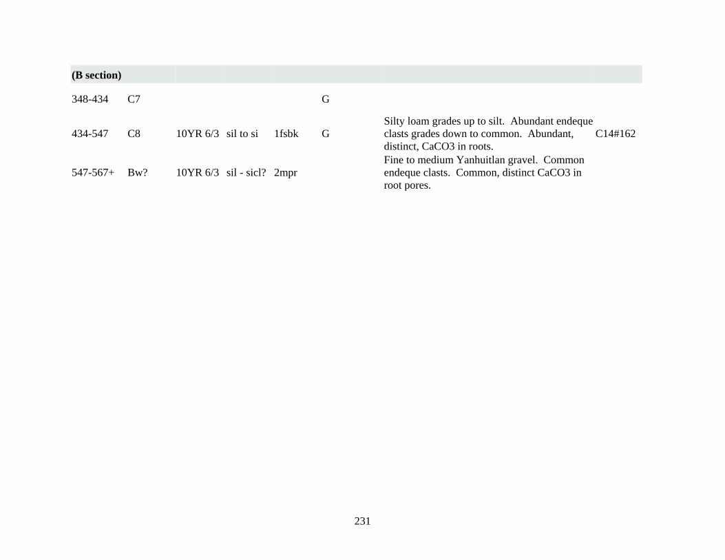
231
(B section)
348-434 C7 G
434-547 C8 10YR 6/3 sil to si 1fsbk G
Silty loam grades up to silt. Abundant endeque
clasts grades down to common. Abundant,
distinct, CaCO3 in roots.
C14#162
547-567+ Bw? 10YR 6/3 sil - sicl? 2mpr
Fine to medium Yanhuitlan gravel. Common
endeque clasts. Common, distinct CaCO3 in
root pores.

232
Table II.d. Island Site Profile Description
Depth (cm) Horizon Color
(Dry) Texture Structure Boundary Remarks
C-14
Samples
(A Section) SE EDGE OF ISLAND
0-35 cm A 7.5YR
5/2 csl
moderate
granular clear
Normally graded coarse sandy loam at base.
Sandy loam at top.
35-76 cm C1 10YR 6/2 (p)sl single
grain abrupt
Thinly bedded, both gravel and sand lenses,
few cobbles. Many endeque clasts. Many
Yanhuitlan clasts.
C14#18
MAIN
PROFILE *All profile has filaments except A and C1.
0-37 cm A 7.5YR 5/2 fsl moderate
granular clear
Normally graded coarse sandy loam at base.
Sandy loam at top.
37-78 cm C1 10YR 6/2 sl massive
(sg?) abrupt
Thinly bedded with few gravel lenses. There
are endeque and Yanhuitlan clasts.
78-111 cm Ab1 10YR 5/1 sil 2msbk gradual
Horizon somewhat transitional to underlying
Ab2. Upper 10 cm slightly darker. Few
medium gravel clasts. Thin humic clay films
coating medium gravel clasts.
111-182 cm Ab2 10YR 3/1 sil 3cgr +
3vcsbk gradual
Common granuals, some of which are endeque.
Few very fine filaments of CaCO3 and root
pores.
C14#15
182-225 cm C2 10YR 7/2 sil 3cpr abrupt Few endeque granuals. Charcoal sample (14C
# 13) at 223-225 cm. C14#13
225-263 cm C3 10YR 7/2 sl/sicl/sil 3cpr abrupt
Many endeque clasts. Stratified beds ranging
from endeque rich sandy loam with gravel to
silty clay loam beds. Includes reworked

233
pottery sherds. Includes 1-2 cm thick charcaol
lens 245-249 cm deep. Charcoal lens is ashy.
263-300 cm C4 10YR 7/2 sil 3mpr clear Very few Yanhuitlan and endeque clasts.
300-335 cm Ab1' 10YR 5/2 sicl 3mpr gradual
Very few Yanhuitlan and endeque clasts.
Charcoal sample (14C # 14) at 324-330 cm.
Few thin granular beds near base, probably
endeque?
C14#14
335-430 cm Ab2' 10YR 4/2 sicl 3cpr diffuse
(ABC) Very few endeque clasts. Pot sherd
recovered. Includes rock cluster 5 m NW of
profile.
430-470 cm Ab3' 10YR 5/3 sil 2msbk clear Very few endeque clasts.
470-484 cm C5 10YR 7/3 sil massive abrupt Common CaCO3 concretions, possibly
transported Yanhuitlan beds.
(B Section) 2.30 m NW of Main Profile
484-610 cm Ab" 10YR 4/2 l 1msbk very abrupt
536-550 cm particularly gravelly zone,
sampled separately. (Pulse of sediment in
swale?) (Horizon paleochannel fills that grade
up to ABC?) Charcoal sample (14C# 17) at
580-590 cm. Weakly stratified with thick and
thin beds. Some beds include abundant
endeque. Gravel, few thin silt lenses. Gravel
beds very poorly sorted within matrix.
C14#16,
#17, #19
610-640 cm C6 10YR 7/3 sil massive massive Suggestive of reworked Yanhuitlan bedrock.
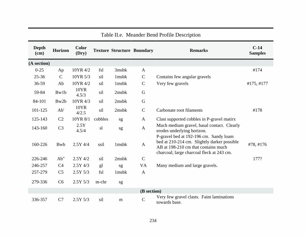
234
Table II.e. Meander Bend Profile Description
Depth
(cm) Horizon
Color
(Dry) Texture Structure Boundary Remarks
C-14
Samples
(A section)
0-25 Ap 10YR 4/2 fsl 3msbk A #174
25-36 C 10YR 5/3 sil 1msbk C Contains few angular gravels
36-59 Ab 10YR 4/2 sil 1msbk C Very few gravels #175, #177
59-84 Bw1b 10YR
4.5/3 sil 2msbk G
84-101 Bw2b 10YR 4/3 sil 2msbk G
101-125 Ab' 10YR
4/2.5 sil 2msbk C Carbonate root filaments #178
125-143 C2 10YR 8/1 cobbles sg A Clast supported cobbles in P-gravel matirx
143-160 C3 2.5Y
4.5/4 sl sg A
Much medium gravel, basal contact. Clearly
erodes underlying horizon.
160-226 Bwb 2.5Y 4/4 ssil 1msbk A
P-gravel bed at 192-196 cm. Sandy loam
bed at 210-214 cm. Slightly darker possible
AB at 198-210 cm that contains much
charcoal; large charcoal fleck at 243 cm.
#78, #176
226-246 Ab" 2.5Y 4/2 sil 2msbk C 177?
246-257 C4 2.5Y 4/3 gl sg VA Many medium and large gravels.
257-279 C5 2.5Y 5/3 fsl 1msbk A
279-336 C6 2.5Y 5/3 m-chr sg
(B section)
336-357 C7 2.5Y 5/3 sil m C Very few gravel clasts. Faint laminations
towards base.

235
357-374 C8 2.5Y
4.5/3 sil m A
Contains many vesicles, as if incipient A
horizon.
374-427 C9 2.5Y 5/3 sil 1msbk C Contains a flood gravel bed at 405-410 cm
depth.
427-473 C10 2.5Y 5/3 s sg VA
Plane bedded rhythmites, gravelly sand
graded up to fine sand (about 5-6 cm),
contains coarse gravel and cobbles elsewhere
on outcrop. Groundwater preculating in zone
under underlying silty loam unit. Erosionally
truncated underlying unit.
#183
473-592 2Ab1 2.5Y 4/2 sicl 2msbk C
Ocassional angular gravels, lens of cobble to
left of main profile. Interpreted as reworked
culural material (little charcoal). Many fine
CaCO3 nodules in upper 30 cm.
#94, #181, #182
592-645 2Ab2 2.5Y 5/2 sicl 3copr A
Abundant, fine-medium gravel, somewhat
bedded. Medium carbonate nodules at 600-
615 cm. Prominent cobble layer at base at
629-645 cm laterally extensive gravelly zone
in zone that interfingers L-B.
#93
645-775 Btb 2.5Y 5/2 sic 3vcpr
Contains Mk films on ped faces. Clay films
which gradually diminish towards base. Lots
of time represented by this horizon. A
prominent L-B structure is upstream (left in
photos) from this profile at 700-750 cm.
#84, #85, #92,
#180
775-850+ C11 2.5Y 5/4 l (sl at
base) m
Abundant charcoal, classic fining upward
sequence. #179

236
Table II.f. Victor’s Lama-Bordo Profile Description
Depth (cm) Horizon Color
(Dry) Texture Structure Boundary Remarks
C-14
Samples
(A Section)
0-65 cm C1 10YR 5/2 grl 3mgr abrupt plowed. Weakly stratified with fine to medium
gravel in lower half.
65-90 cm Ab 10YR 4/2 sil 3cogr gradual (14C#109) bulk C14#109
90-142 cm Bw 10YR
4.5/1 sil 1cosbk diffuse
common, fine gravel throughout. No bedding,
massive. (14C# 110) C14#111
142-188 cm Ab' 10YR 4/1 hsil 3msbk diffuse fine CaCO3 filaments throughout rootlet holes.
(14C# 110) (potsherd, chert flake at 160 cm) C14#110
(B Section)
188-232 cm Bw' 10YR 5/2 sil 3mgr clear CaCO3 in rootlets and faint CaCO3 on ped faces C14#113
232-251 cm C2 10YR 5/1 grl m clear lots of endeque granules. Freguent large gravel
and cobble
251-306 cm C3 10YR 5/2 sil 3copr clear
lots of endeque granules. Freguent large gravel
and cobble. CaCO3 infilling rootlets and ped
faces (as above)
306-336+
cm C4
see C4 in
C section lots of endeque granules (14C# 110) C14#112
(C Section)
306-431 cm C4 10YR 5/2 sil 1copr to m clear CaCO3 infillings of rootlets, NOT ped faces C14#116
431-480 cm Ab' 10YR 4/1 hsil 1fgr to m gradual very few CaCO3 infillings, many endeque
granules
C14#114,
#115,
#117,
#119
(D Section)
480-517 cm C5 10YR 4/2 l m clear abundant endeque granules. Fine, medium
gravel
517-540 cm C6 10YR 5/3 l gravel sg very abrupt

237
540 - see C7
in E section C7 10Yr 6/2 ssi
laminated
and thinly
saturated
few thing beds of reworked endeque C14#118
(E Section)
540-569 cm C7 abrupt
569-590 cm Ab'' 10YR 4/1 sil 2msbk clear
few endeque granules. Few rootlet fillaments of
CaCO3. corresponds to very top of intact of
preserved lama-bordo rocks.
590-700 cm C8
10YR 4/1,
10YR 5/2,
10YR 4/2
si to grsil thinly
stratified see section F
typical 5-15 cm beds of laminated silts to poorly
sorted gravelly silty loam C14#120
(F Section)
700-900 cm C8 diffuse
(cont. from above) and with depth below 8m
(especially below 8m) increasing frequency of
sandy loam beds and sandy gravel beds. * All
planar beds; do not exhibit cross-beds.
C14#121,
#122,
#129
(G Section)
900-1123
cm C9 very abrupt
as above in C8, but with prominent 5- 15cm
thick beds of rounded endeque and Yanhuitlan
gravels. All planar beds. Many, distinct,
normally graded beds. D90 size typically 4-5
cm. Endeque gravel well rounded vs. Yanhuitlan
gravel subangular and angular. Basal bed is
laminated silty sand, 1100-1123 cm. (seperate
bags of gravel, Gravel sample 1: 960-970 cm,
and Gravel sample 2: 1010-1020 cm.) Some
beds are distinctly graded from gravel up to silty
clay and as indeed are rhythmites.
***Absolutely no evidence of human
disturbance in rhythmite beds.
C14#128

238
1123-1164
cm Ab1''
10YR 4/2
and 10YR
6/4
sil 1msbk clear
many inclusions of endeque granules. 10YR 6/4
beds may be krotovina and possibly old plow
zone.
C14#124,
#127
1164-1200
cm Ab2'' 10YR 3/2 sil 1msbk clear
definite 10YR 6/4 krotovina, very few endeque
granules
C14#123,
#125
1200-1230
cm Ab3''k
same as above, but with prominent CaCO3
filaments C14#126

239
Table II.g. Confluence Profile Description
Depth (cm) Horizon Color
(Dry) Texture Structure Boundary Remarks
C-14
Samples
(A Section)
0-19 A 10YR 4/2 sil 2msbk G
19-32 C1 10YR 5/3 sil 1msbk G graded towards sand at base
32-41 C2 10YR 5/4 ls sg A
41-53 Ab 10YR 5/2 sil 2msbk G top 5 cm bulk #148
53-64 C3 10YR
4/5.2 sil m C very faint laminae
64-83 Ab' 10YR 4/2 sil 2msbk C top 5 cm bulk #147
83-93 Bw1 10YR
4/2.5 sil 2msbk C
thin discontinuous CaCO3 on ped faces and root
filaments
93-155 Bw2 10YR
3.5/3 sil 2msbk G
thin discontinuous CaCO3 on ped faces and root
filaments
155-194 BC 10YR 5/3 sil 1cosbk to
m C BC due to color??
194-204 Ab''
(B Section)
194-222 Ab" 10YR 4/2 sil 2vcosbk G
#149,
#150,
#152
222-250 Bwb" 10YR 4/3 sil 2cosbk G
250-273 BCb" 10YR 4/3 sil 1cosbk to
m A
273-287 C4 10YR 6/3 fine sand laminated A faint planar bed laminations #151
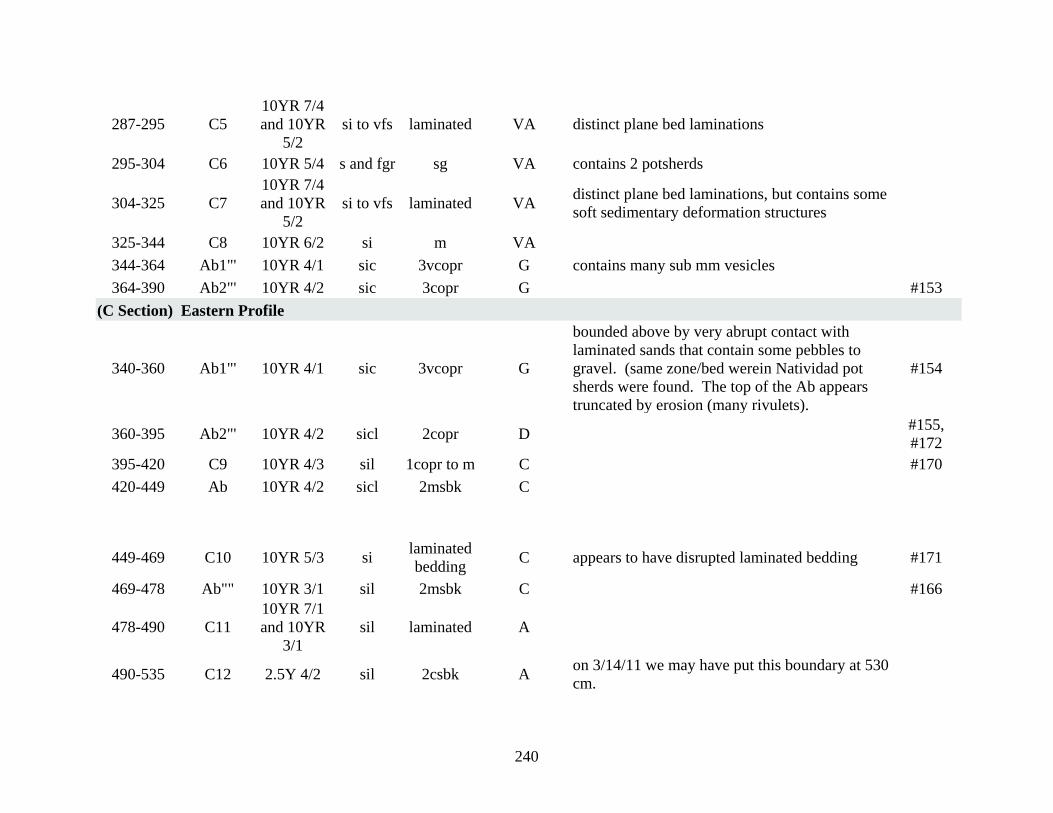
240
287-295 C5
10YR 7/4
and 10YR
5/2
si to vfs laminated VA distinct plane bed laminations
295-304 C6 10YR 5/4 s and fgr sg VA contains 2 potsherds
304-325 C7
10YR 7/4
and 10YR
5/2
si to vfs laminated VA distinct plane bed laminations, but contains some
soft sedimentary deformation structures
325-344 C8 10YR 6/2 si m VA
344-364 Ab1"' 10YR 4/1 sic 3vcopr G contains many sub mm vesicles
364-390 Ab2"' 10YR 4/2 sic 3copr G #153
(C Section) Eastern Profile
340-360 Ab1"' 10YR 4/1 sic 3vcopr G
bounded above by very abrupt contact with
laminated sands that contain some pebbles to
gravel. (same zone/bed werein Natividad pot
sherds were found. The top of the Ab appears
truncated by erosion (many rivulets).
#154
360-395 Ab2"' 10YR 4/2 sicl 2copr D #155,
#172
395-420 C9 10YR 4/3 sil 1copr to m C #170
420-449 Ab 10YR 4/2 sicl 2msbk C
449-469 C10 10YR 5/3 si laminated
bedding C appears to have disrupted laminated bedding #171
469-478 Ab"" 10YR 3/1 sil 2msbk C #166
478-490 C11
10YR 7/1
and 10YR
3/1
sil laminated A
490-535 C12 2.5Y 4/2 sil 2csbk A on 3/14/11 we may have put this boundary at 530
cm.

241
535-570 C13 2.5Y 6/3 ssil laminated VA #156,
#157
570-591 C14 2.5Y 5/3 sil 2msbk G darker topset at 570-573 cm sampled on 3/14/11
for C14
591-612 C15 2.5Y 5/3 ssil
m and
thinly
bedded
C
612-723 C16
2.5Y 7/4
(si) and
2.5Y 5/3
(sil)
si and sil
laminated
and thinly
bedded
G
contains a few beds of distinctly laminated silts
and fine sands, otherwise there is lamination
throughout, but most of it is deformed/disturbed
abundant large pieces of charcoal (collected
some). Few dark beds (10YR 4/2) are present,
but not buried A horizons.
#168,
#169,
#173
723-765 C17 2.5Y 5/3 sil 1msbk to
m C
exhibits faint thin bedding and few organic
lenses #167
765-800 C18 2.5Y 5/3 sl m exhibits faint thin bedding

242
Table II.h. Cuganda Sur Profile Description
Depth (cm) Horizon Color
(Dry) Texture Structure Boundary Remarks
C-14
Samples
0-22 A 10YR 4/2 sil 1fgr VA Endeque. F, d, S-I CaCO3 nodules (2 mm gr
sized). From break up of endeque #234
22-39 Ck 10YR 7/2 sil 1fsbk A small endeque/nodules? Layers/massive-
petrocalcic?
39-58 Ck2 10YR 6/2 sil 2fsbk C very similar to above only more structure
58-77 C 10YR 6/3 sil 1fsbk G f, f-med gr Endeque clasts (YAN beds derived
C)
77-131 C2 10YR 5/4 sil 2msbk C
very similar to above only stronger structure
and more abundant Endeque clasts towards
bottom. C-a, med to co gr Endeque clasts. Vf,
f-med Yanhuitlan clasts.
131-152 C3 10YR 5//2 sil 2msbk VA c, f-m Endeque clasts. Vf, f gr, Yanhuitlan
clasts
152-195 Ab 10YR 4/1 sicl 2mwedge G c, p, CF on PF. F, d, masses, I, CaCO3 on PF. #235
195-273 Ab2 10YR 4/2 sicl 2mpr C
c-a, p, strong CF on PF. C, p, med-co CaCO3
masses I-S on PF. F, d, Mg dep on PF. F, d,
slickenslides. Few, very small charcoal flecks.
#236
273-300 AC 10YR 4/2 sil 2fpr
c, d, CF on PF. F, f, CaCO3 on PF. F, d,
CaCO3 in RP. Organic fill on PF, root
disturbance. F, med Endeque clasts

243
Table II.i. Inguiro Site Profile Description
Depth (cm) Horizon Color
(Dry) Texture Structure Boundary Remarks
C-14
Samples
(A Section)
0-22 A 10YR 5/2 sl 2fgr C gravel-cobble colluvial inclusions
22-39 C 10YR 5/2 vfsl 2cogr A c, f-co Endeque clasts. F-c gravel- cobble
colluvial inclusions
39-65 2Ab 10YR 4/2 sil 3cogr C c,d CaCO3 on ped faces C14#239
65-81 2Ab2 10YR 5/2 sil 3cogr A f, d, Ca CO3 on ped faces. F, gravel - cobble
colluvial inclusions
81-111 C2 10YR 5/3 m 1msbk VA f, d, CaCO3 on root pores. F, f, CaCO3 on some
ped faces. F, coare gravel colluvial inclusions.
111-133 C3 10YR 5/3 si/cogr sg VA
p, yanhuitlan clasts. F, endeque clasts. Biggest
clast is 5 x 5 cm. Silty layer bounded by 2 gravel
layers. The lower gravel layer fines up to the
silty layer.
133-165 C4 2.5Y 5/3 sl m D lenses of cos-coarse gravel in matrix of silt. C14#200
165-190 2Ab' 2.5Y 4/2 sil 1msbk A patches of diffuse boundary 2.2Y 5/3. c,p,
CaCO3 in root pores. F,f Yanhuitlan clasts. C14#238
190-260 2Ab2' 1.5Y 4/2 sil 3mweg C f, p, CaCO3 in root pores. F,f, CaCO3 on some
ped faces. F,f, endeque clasts. C14#237
260-302 2Ab3' 2.5Y 4/2;
2.5Y 6/3 sil 3fp2 A f, f, CaCO3 on root pores
302-359 2Ab4' 2.5Y 4/2;
2.5Y 6/3 sil 2fp2 G
f, p, CaCO3 in root pores. F,vf-f Endeque and
Yanhuitlan clasts.

244
359-403 AC SEE
BELOW
C14#201,
#202
(B Section)
372-412 AC 10YR 4/1 sil 2fp2 C f,d, CaCO3 in root pores
412-424 Ck 10YR 5/2 sil 2vfpr G f, coarse endeque clasts. F, d, I CaCO3 masses.
F, p, CaCO3 in root pores.
424-437 C5 10YR 6/2 sil-fs m VA f, f-med Endeque clasts. F, f, Yanhuitlan clasts
437-442 C6 2.5YR 6/2 fs, f-m gr sg VA lenses of sand-gravel sized Yanhuitlan clasts. F, f
endeque clasts.
442-473 C7 2.5YR 6/3 ls m VA f, d, I, CaCO3 noduels. C, f, endeque and
Yanhuitlan clasts
473-530 C8 10YR 6/3;
2.5YR 6/2 cos; fs-sil
laminated,
fining
upward
seq
VA fluvial beds, bands of beds with few f-co sized
endeque clasts, and common Yanhuitlan clasts
530-548 C9 10YR 6/2 fs- stones sg VA coarsening upward bed. Mixed detrital
548-550+ SEE
BELOW
(C Section)
548-589 Bw 7.5YR 6/3 sil 2fsbk A F,D, CaCO3 in root pores. F,d CaCO3 on ped
faces
589-610 Bk 7.5YR 7/2;
7.5YR 8/1 sil 2fsbk A c,p, CaCO3 on ped faces
610-643 Ck 7.5YR 7/2 sil 1fsbk A f,d, S, CaCO3 nodules
643-716 C10 7.5YR 7.3 s-cos m/1fsbk C fluvial deposits, with coarse sand- gravel sized
endeque and Yanhuitlan clasts
716-759 2Bt 7.5YR 5/3 si-cogr sg,
laminated VA c,p,f-med, I CaCO3 masses
759-792 C11 7.5YR 7/3 sicl 3mpr C (color is moist) c, f, endeque clasts. F, m
Yanhuitlan clasts. C,d, cf on ped faces

245
792-823 C12 7.5YR 7/3 fsl 1msbk A f,f, CaCO3 in root pores. Cf endeque and
Yanhuitlan clasts
823-925 C13
10YR 4/3;
10YR 5/4;
10YR 5/3
cl m/1msbk A
pathy. F, d, f, I CaCO3 masses at 852-853 cm
and 110 lenses of endeque and carbonate
nodules. (coarse rocks are between 2-4 cm)
925-950+ C14 2.5Y 5/3 sic m non-homogenous
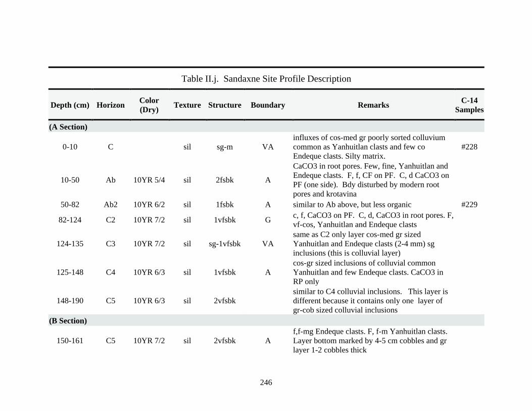
246
Table II.j. Sandaxne Site Profile Description
Depth (cm) Horizon Color
(Dry) Texture Structure Boundary Remarks
C-14
Samples
(A Section)
0-10 C sil sg-m VA
influxes of cos-med gr poorly sorted colluvium
common as Yanhuitlan clasts and few co
Endeque clasts. Silty matrix.
#228
10-50 Ab 10YR 5/4 sil 2fsbk A
CaCO3 in root pores. Few, fine, Yanhuitlan and
Endeque clasts. F, f, CF on PF. C, d CaCO3 on
PF (one side). Bdy disturbed by modern root
pores and krotavina
50-82 Ab2 10YR 6/2 sil 1fsbk A similar to Ab above, but less organic #229
82-124 C2 10YR 7/2 sil 1vfsbk G c, f, CaCO3 on PF. C, d, CaCO3 in root pores. F,
vf-cos, Yanhuitlan and Endeque clasts
124-135 C3 10YR 7/2 sil sg-1vfsbk VA
same as C2 only layer cos-med gr sized
Yanhuitlan and Endeque clasts (2-4 mm) sg
inclusions (this is colluvial layer)
125-148 C4 10YR 6/3 sil 1vfsbk A
cos-gr sized inclusions of colluvial common
Yanhuitlan and few Endeque clasts. CaCO3 in
RP only
148-190 C5 10YR 6/3 sil 2vfsbk
similar to C4 colluvial inclusions. This layer is
different because it contains only one layer of
gr-cob sized colluvial inclusions
(B Section)
150-161 C5 10YR 7/2 sil 2vfsbk A
f,f-mg Endeque clasts. F, f-m Yanhuitlan clasts.
Layer bottom marked by 4-5 cm cobbles and gr
layer 1-2 cobbles thick
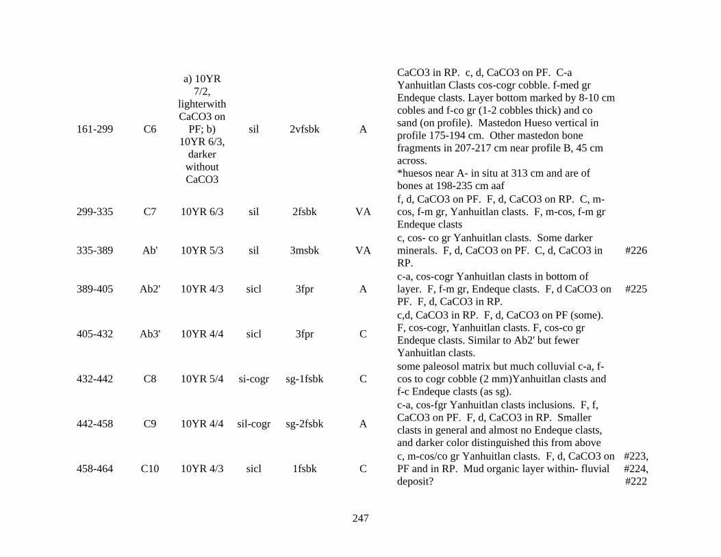
247
161-299 C6
a) 10YR
7/2,
lighterwith
CaCO3 on
PF; b)
10YR 6/3,
darker
without
CaCO3
sil 2vfsbk A
CaCO3 in RP. c, d, CaCO3 on PF. C-a
Yanhuitlan Clasts cos-cogr cobble. f-med gr
Endeque clasts. Layer bottom marked by 8-10 cm
cobles and f-co gr (1-2 cobbles thick) and co
sand (on profile). Mastedon Hueso vertical in
profile 175-194 cm. Other mastedon bone
fragments in 207-217 cm near profile B, 45 cm
across.
*huesos near A- in situ at 313 cm and are of
bones at 198-235 cm aaf
299-335 C7 10YR 6/3 sil 2fsbk VA
f, d, CaCO3 on PF. F, d, CaCO3 on RP. C, m-
cos, f-m gr, Yanhuitlan clasts. F, m-cos, f-m gr
Endeque clasts
335-389 Ab' 10YR 5/3 sil 3msbk VA
c, cos- co gr Yanhuitlan clasts. Some darker
minerals. F, d, CaCO3 on PF. C, d, CaCO3 in
RP.
#226
389-405 Ab2' 10YR 4/3 sicl 3fpr A
c-a, cos-cogr Yanhuitlan clasts in bottom of
layer. F, f-m gr, Endeque clasts. F, d CaCO3 on
PF. F, d, CaCO3 in RP.
#225
405-432 Ab3' 10YR 4/4 sicl 3fpr C
c,d, CaCO3 in RP. F, d, CaCO3 on PF (some).
F, cos-cogr, Yanhuitlan clasts. F, cos-co gr
Endeque clasts. Similar to Ab2' but fewer
Yanhuitlan clasts.
432-442 C8 10YR 5/4 si-cogr sg-1fsbk C
some paleosol matrix but much colluvial c-a, f-
cos to cogr cobble (2 mm)Yanhuitlan clasts and
f-c Endeque clasts (as sg).
442-458 C9 10YR 4/4 sil-cogr sg-2fsbk A
c-a, cos-fgr Yanhuitlan clasts inclusions. F, f,
CaCO3 on PF. F, d, CaCO3 in RP. Smaller
clasts in general and almost no Endeque clasts,
and darker color distinguished this from above
458-464 C10 10YR 4/3 sicl 1fsbk C
c, m-cos/co gr Yanhuitlan clasts. F, d, CaCO3 on
PF and in RP. Mud organic layer within- fluvial
deposit?
#223,
#224,
#222
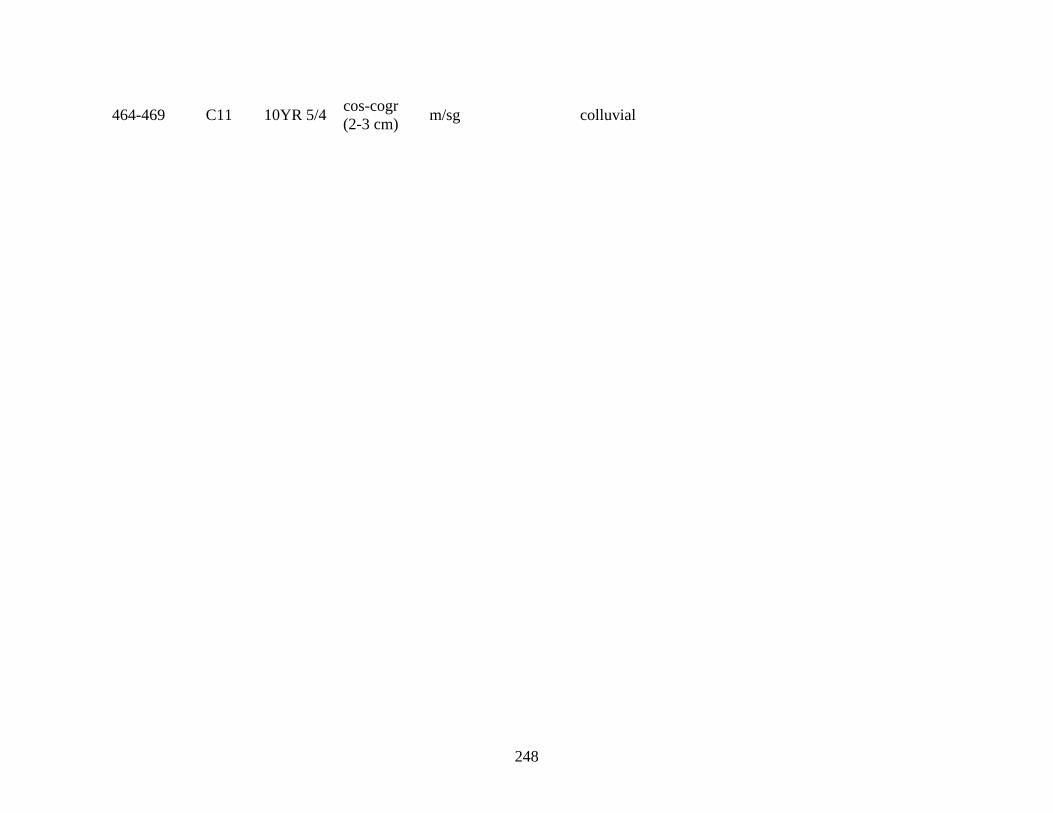
248
464-469 C11 10YR 5/4 cos-cogr
(2-3 cm) m/sg colluvial

249
Table II.k. Sauce Site Profile Description
Depth (cm) Horizon Color
(Dry) Texture Structure Boundary Remarks
C-14
Samples
PROFILE 1
550-552 C1 10YR 5/3 fgr-fsi sg A fining up sequence- here only sampled gravel-
sand but above nail it continues as m-fs and si.
552-580 C2 10YR 5/4 gr (~5
cm)-sil
sg-
massive C
finign upward sequence at bottom mainly
gravel fines up to sil which has more structure
though weak. Sil also has CaCO3 on PF and
RP. ~5 cm band of reddish clay (subsample of
sil). At 2-11 cm some cross trough bedding
noticeable to right.
580-603 C3 10YR 5/2 gr (~10
cm)-fsl
sg-
massive VA
large cut at bottom fining up to fs-sl, followed
by two more fining upward sequences to top
with noteable cross trough bedding. Sl with
structure contains charcoal. More structure in
part of sl; sl also contains CaCO3 on RP and
PF. In the gravel (~2 cm max) to fsl layers the
bedding is very apparent, but only in the
bottom gravel part is the cross trough bedding
clear. These beds contain some clay chunks
603-613 C4 10YR 6/2 fg-sl sg-
massive VA
fining up sequence. No sedimentary structures,
thus plain beds. Towards top in the sl it is
more massive. The sl also contains some
charcoal but it is not noticeable across whole
layer. More structure or more consolidated
than in layers to bottom and top.
613-650 C5 10YR 5/4
gr (~2
cm) - sl
(or sil)
sg/bedding A
Around 5 main fining upward sequences and
some up to sl and others sil. The top cm
consists of sil which is above the sl with
CaCO3 in RP and on PF and more massive
structure (possible 1fsbk). This sub-layer has
#296
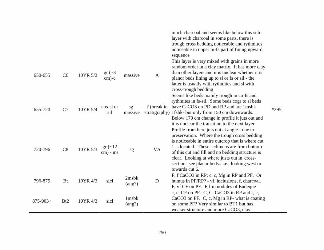
250
much charcoal and seems like below this sub-
layer with charcoal in some parts, there is
trough cross bedding noticeable and rythmites
noticeable in upper m-fs part of fining upward
sequence
650-655 C6 10YR 5/2 gr (~3
cm)-c massive A
This layer is very mixed with grains in more
random order in a clay matrix. It has more clay
than other layers and it is unclear whether it is
planor beds fining up to sl or fs or sil - the
latter is usually with rythmites and sl with
cross-trough bedding
655-720 C7 10YR 5/4 cos-sl or
sil
sg-
massive
? (break in
stratigraphy)
Seems like beds mainly trough in co-fs and
rythmites in fs-sil. Some beds cogr to sl beds
have CaCO3 on PD and RP and are 1msbk-
1fsbk- but only from 150 cm downwards.
Below 170 cm change in profile it juts out and
it is unclear the transition to the next layer.
#295
720-796 C8 10YR 5/3 gr (~12
cm) - ms sg VA
Profile from here juts out at angle - due to
preservation. Where the trough cross bedding
is noticeable in entire outcrop that is where cut
1 is located. These sedimens are from bottom
of this cut and fill and no bedding structure is
clear. Looking at where justs out in 'cross-
section" see planar beds.. i.e., looking west or
towards cut 6.
796-875 Bt 10YR 4/3 sicl 2msbk
(ang?) D
F, f CaCO3 in RP; c, c, Mg in RP and PF. Or
humus in PF/RP? - vf, inclusions, f, charcoal.
F, vf CF on PF. F,f-m nodules of Endeque
875-903+ Bt2 10YR 4/3 sicl 1msbk
(ang?)
c, c, CF on PF. C, C, CaCO3 in RP and f, c,
CaCO3 on PF. C, c, Mg in RP- what is coating
on some PF? Very similar to BT1 but has
weaker structure and more CaCO3, clay
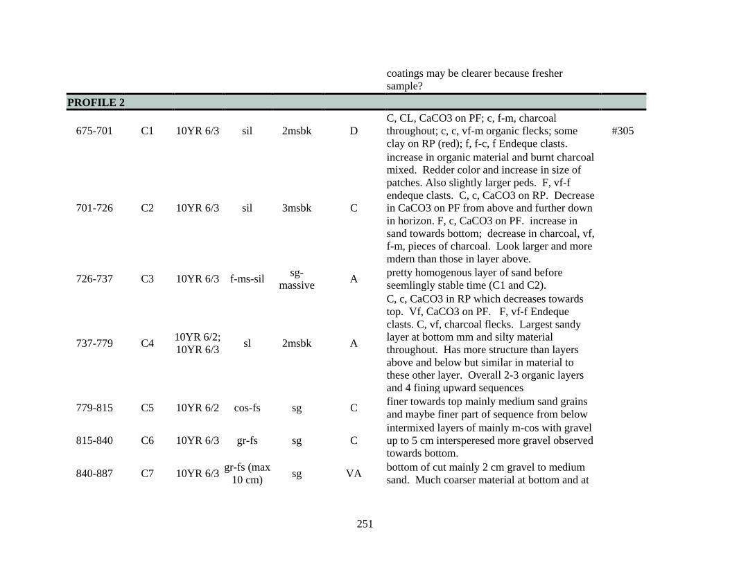
251
coatings may be clearer because fresher
sample?
PROFILE 2
675-701 C1 10YR 6/3 sil 2msbk D
C, CL, CaCO3 on PF; c, f-m, charcoal
throughout; c, c, vf-m organic flecks; some
clay on RP (red); f, f-c, f Endeque clasts.
#305
701-726 C2 10YR 6/3 sil 3msbk C
increase in organic material and burnt charcoal
mixed. Redder color and increase in size of
patches. Also slightly larger peds. F, vf-f
endeque clasts. C, c, CaCO3 on RP. Decrease
in CaCO3 on PF from above and further down
in horizon. F, c, CaCO3 on PF. increase in
sand towards bottom; decrease in charcoal, vf,
f-m, pieces of charcoal. Look larger and more
mdern than those in layer above.
726-737 C3 10YR 6/3 f-ms-sil sg-
massive A
pretty homogenous layer of sand before
seemlingly stable time (C1 and C2).
737-779 C4 10YR 6/2;
10YR 6/3 sl 2msbk A
C, c, CaCO3 in RP which decreases towards
top. Vf, CaCO3 on PF. F, vf-f Endeque
clasts. C, vf, charcoal flecks. Largest sandy
layer at bottom mm and silty material
throughout. Has more structure than layers
above and below but similar in material to
these other layer. Overall 2-3 organic layers
and 4 fining upward sequences
779-815 C5 10YR 6/2 cos-fs sg C finer towards top mainly medium sand grains
and maybe finer part of sequence from below
815-840 C6 10YR 6/3 gr-fs sg C
intermixed layers of mainly m-cos with gravel
up to 5 cm intersperesed more gravel observed
towards bottom.
840-887 C7 10YR 6/3 gr-fs (max
10 cm) sg VA
bottom of cut mainly 2 cm gravel to medium
sand. Much coarser material at bottom and at

252
bottom intermixed with older gravel layer.
Maybe copart of fining up sequence from C8 to
C7
887-892 C8 10YR 6/2 fgr-fs sg VA mainly coarse sand- part of older gr-s layer
which later cut cuts into
892-894 C9 10YR 6/3 ms-si sg VA fining upward sequence and dated ms-silt
894-910 C10 10YR 6/3 sil-fs sg C rythmite beds still noticeable but cemented
mainly silt - very weak strcutre started
910-930 Ab1 10YR 5/1 sl 2mgr D
"organic layer" cumulic A in paleoswale
allowed time to develop weak structure. C, vf-
f Endeque clasts. C, vf flecks of charcoal; f-c,
vf-m Yanhuitlan and volcanic clasts; f clay in
RP- red.
930-989 AC 10YR 5/1 gr-s sg (1fgr) VA
"part of cumulic A" but this layer consists of
mainly gravel to sand with 2-3 intermittent
darker layers- of organic material or well
developed A- (i.e., periods of stability)?
Organic A layers here are weaker than above
and finer with many inclusions. Mainly C12
layers of fs-fgr up to 3 cm max. Around 5 fill
layers of mainly fs and cos.
989-1002 Ab' 10YR 6/2 sl 2mgr VA
part of same cumulic horizon as Ab1 bottom
towards righ combines into 1 (i.e., towards cut
edge or hillslope and tribfurcates towards
center of paleoarroyo
1002-1045 C11 10YR 6/3 si-gr sg C
fining upward sequence from gravel (majority
between 2-5 cm) upper gravel and sand layers
(mainly ms-gr up to 2 cm). Ab at top and
bottom is a silty layer containing C-14
material. Probably antoher set of fining
upward sequences starting from C12.
1045-1089 C12 10YR 6/3 fs-gr sg VA several layers of gr-s at bottom of fill (between
12-20 cm is size range for larger gravel) and

253
mainly m-cos and between 2-5 cm gravel. To
right and left of profile are intermittent with
silty layer and evidence for cross-trough
bedding
1089-1097+ 2Ab 10YR 4/1 sil 2msbk …
c,c, CF on PF; humic (or Mg??) - coatings on
PF. F, f-m Endeque, Yanhuitlan and volcanic
clasts. Cery late color for A - post
pedogenically altered?
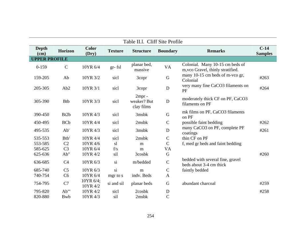
254
Table II.l. Cliff Site Profile
Depth
(cm) Horizon
Color
(Dry) Texture Structure Boundary Remarks
C-14
Samples
UPPER PROFILE
0-159 C 10YR 6/4 gr- fsl planar bed,
massive VA
Colonial. Many 10-15 cm beds of
m,vco Gravel, thinly stratified.
159-205 Ab 10YR 3/2 sicl 3copr G many 10-15 cm beds of m-vco gr,
Colonial #263
205-305 Ab2 10YR 3/1 sicl 3copr D very many fine CaCO3 filaments on
PF #264
305-390 Btb 10YR 3/3 sicl
2mpr -
weaker? But
clay films
D moderately thick CF on PF, CaCO3
filaments on PF
390-450 Bt2b 10YR 4/3 sicl 3msbk G mk films on PF, CaCO3 filaments
on PF
450-495 BCb 10YR 4/4 sicl 2msbk C possible faint bedding #262
495-535 Ab' 10YR 4/3 sicl 3msbk D many CaCO3 on PF, complete PF
coatings #261
535-553 Btb' 10YR 4/4 sicl 2msbk C thin CF on PF
553-585 C2 10YR 4/6 sl m C f, med gr beds and faint bedding
585-625 C3 10YR 6/4 f/s m VA
625-636 Ab" 10YR 4/2 sil 3cosbk G #260
636-685 C4 10YR 6/3 si m/bedded C bedded with several fine, gravel
beds about 3-4 cm thick
685-740 C5 10YR 6/3 si m C faintly bedded
740-754 C6 10YR 6/4 mgr to s indv. Beds A
754-795 C7 10YR 6/4;
10YR 4/2 si and sil planar beds G abundant charcoal #259
795-820 Ab"' 10YR 4/2 sicl 2cosbk D #258
820-880 Bwb 10YR 4/3 sil 2msbk C
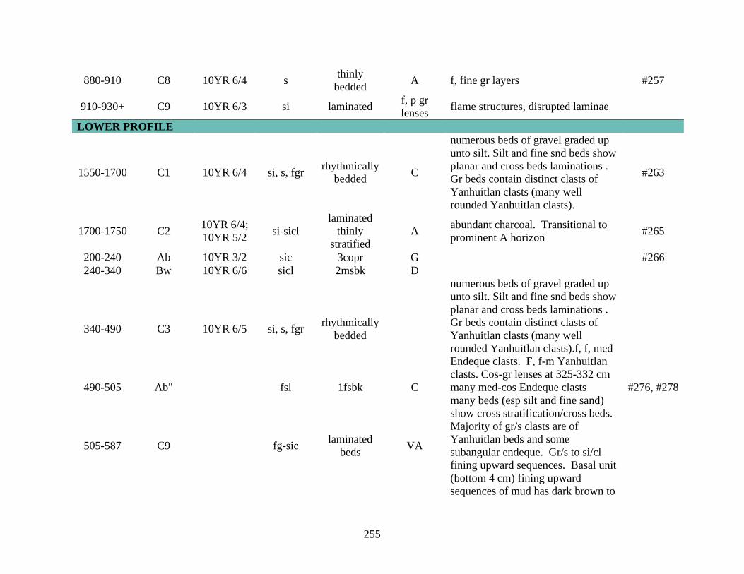
255
880-910 C8 10YR 6/4 s thinly
bedded A f, fine gr layers #257
910-930+ C9 10YR 6/3 si laminated f, p gr
lenses flame structures, disrupted laminae
LOWER PROFILE
1550-1700 C1 10YR 6/4 si, s, fgr rhythmically
bedded C
numerous beds of gravel graded up
unto silt. Silt and fine snd beds show
planar and cross beds laminations .
Gr beds contain distinct clasts of
Yanhuitlan clasts (many well
rounded Yanhuitlan clasts).
#263
1700-1750 C2 10YR 6/4;
10YR 5/2 si-sicl
laminated
thinly
stratified
A abundant charcoal. Transitional to
prominent A horizon #265
200-240 Ab 10YR 3/2 sic 3copr G #266
240-340 Bw 10YR 6/6 sicl 2msbk D
340-490 C3 10YR 6/5 si, s, fgr rhythmically
bedded
numerous beds of gravel graded up
unto silt. Silt and fine snd beds show
planar and cross beds laminations .
Gr beds contain distinct clasts of
Yanhuitlan clasts (many well
rounded Yanhuitlan clasts).f, f, med
Endeque clasts. F, f-m Yanhuitlan
clasts. Cos-gr lenses at 325-332 cm
490-505 Ab" fsl 1fsbk C many med-cos Endeque clasts #276, #278
505-587 C9 fg-sic laminated
beds VA
many beds (esp silt and fine sand)
show cross stratification/cross beds.
Majority of gr/s clasts are of
Yanhuitlan beds and some
subangular endeque. Gr/s to si/cl
fining upward sequences. Basal unit
(bottom 4 cm) fining upward
sequences of mud has dark brown to

256
black. (non silt but sandy clay rich
has reddish color. )
587-602 C10 med-cogr
sic
laminated
beds A
cross trough bedding, gravel (up to 5
cm) to fs-sic fining upward
sequence. Majority are subangular
Yanhuitlan beds clasts and angular
Endeque clasts.
602-672 C11 fgr-fs laminated
beds VA
upper boundary is a muddy (4 cm
thick) layer is overlain by a cos-fs
layer (about 1 cm thick). From
602- 615 cm are fgr- fs cross trough
bedding. Below this, from 615-652
cm are mixed cross and planar beds
of fgr-fs. Bottom 15-20 cm (from
652-672 cm) contains definite cross
cross trough bedding of gravel and
cobbles (diameter 10 cm). Beds
contain Yanhuitlan and Endeque
angular to rounded clasts.
672-742+ C12
mainly
sicl, also
fining
upward(?-
no) fgr-sic
#274, #275

257
Table II.m. Río Culebra Confluence Profile
Depth
(cm) Horizon
Color
(Dry) Texture Structure Boundary Remarks
C-14
Samples
(A Section)
0-15 A 10YR 5/2 sil 1msbk G
f, d, CaCO3 in RP and PF. C, f-
med, Yanhuitlan and endeque clasts.
(part of cumulic horizon or disturbed
due to modern LB.)
15-49 A2 10YR 5/2 sil 1msbk VA
vf, f-med Endeque clasts. F, d
CaCO3 in RP and PF. Common
Yanhuitlan clasts.
#189
49-72 C 10YR 5/2 fs-cogr laminated s,
m VA
3 fining upward sequences of fs-
cogr of mainly Yanhuitlan clasts,
but includes some Endeque clasts.
72-109 Ab' 10YR 6/2 sil 3cogr G
f, f, CaCO3 on PF and RP. F, f,
Yanhuitlan clasts, f, f, endeque
clasts. Much fewer than in Ab and
Ab2.
#188
109-136 C2 10YR 6/3 sil 1cogr C common, fine- medium Yanhuitlan
clasts. F, f-m endeque clasts.
136-149 C3 10YR 6/3 sil-sg 1mgr A
a, f Yanhuitlan clasts, few, fine-
medium Endeque clasts. Separated
from V above due to the abundance
of Yanhuitlan clasts. Fluvial
deposits.
149-173 C4 10YR 6/3 sil 2cogr D few, fine endeque clasts, and no
Yanhuitlan clasts.
173-190 C5 10YR 6/2;
10YR 6/3 sil/sicl 3cogr/1msbk A
patchy due to diffuce boundary.
Redox features BPF, I, I dif, (10YR
6/4). F, d, CaCO3 in RP.
190-224 Ab" 10YR 5/1 sil 2msbk G f, f, Endeque clasts and f, f,
Yanhuitlan clasts. Some oxidation
#187,
#255
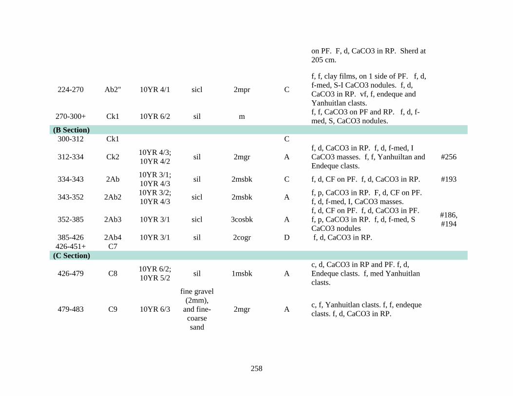
258
on PF. F, d, CaCO3 in RP. Sherd at
205 cm.
224-270 Ab2" 10YR 4/1 sicl 2mpr C
f, f, clay films, on 1 side of PF. f, d,
f-med, S-I CaCO3 nodules. f, d,
CaCO3 in RP. vf, f, endeque and
Yanhuitlan clasts.
270-300+ Ck1 10YR 6/2 sil m f, f, CaCO3 on PF and RP. f, d, f-
med, S, CaCO3 nodules.
(B Section)
300-312 Ck1 C
312-334 Ck2 10YR 4/3;
10YR 4/2 sil 2mgr A
f, d, CaCO3 in RP. f, d, f-med, I
CaCO3 masses. f, f, Yanhuiltan and
Endeque clasts.
#256
334-343 2Ab 10YR 3/1;
10YR 4/3 sil 2msbk C f, d, CF on PF. f, d, CaCO3 in RP. #193
343-352 2Ab2 10YR 3/2;
10YR 4/3 sicl 2msbk A
f, p, CaCO3 in RP. F, d, CF on PF.
f, d, f-med, I, CaCO3 masses.
352-385 2Ab3 10YR 3/1 sicl 3cosbk A
f, d, CF on PF. f, d, CaCO3 in PF.
f, p, CaCO3 in RP. f, d, f-med, S
CaCO3 nodules
#186,
#194
385-426 2Ab4 10YR 3/1 sil 2cogr D f, d, CaCO3 in RP.
426-451+ C7
(C Section)
426-479 C8 10YR 6/2;
10YR 5/2 sil 1msbk A
c, d, CaCO3 in RP and PF. f, d,
Endeque clasts. f, med Yanhuitlan
clasts.
479-483 C9 10YR 6/3
fine gravel
(2mm),
and fine-
coarse
sand
2mgr A c, f, Yanhuitlan clasts. f, f, endeque
clasts. f, d, CaCO3 in RP.

259
483-507 Ck 10YR 6/3;
10YR 6/2
fine to
medium
gravel to
silt
2mgr A
no bedding or laminations. Fining
upward sequences. CaCO3 in root
pores. c, d, f-med, I, CaCO3
masses. c, m, Yanhuitlan clasts. f,
vf, Endeque clasts.
#252
507-516 C10 10YR 6/2 fs-mgr 2mgr A c, f, CaCO3 on PF. f, d CaCO3 in
RP. f, f, Endeque clasts. #253
516-519 C11 10YR 6/3 sil-fs sg C f, p, Yanhuitlan clasts. f, f, endeque
clasts.
519-553 C12 10YR 6/3 fs-fgr 1fgr G
si on bottom coarsesns up and is
overlain by fsl cs- fgr. Above this is
sil and csfs. C, d, CaCO3 in RP.
553-562 2Ab" 10YR 6/3;
10YR 5/3 sil 2fsbk C
f, f, CaCO3 on PF. F, d, CaCO3 in
RP. Silty lenses from 555-557 cm
and from 561-562 cm, which has
1fgr structure. Cumulic A. Color of
CaCO3 in pores is 10YR 7/2.
562-582 2Ab2" 10YR 5/3;
10YR 5/2 sil 1msbk G c, d, CaCO3 in RP and PF. #195
582-598 2Ab3" 10YR 5/3;
10YR 5/2 sil 2msbk G
c, d, CaCO3 in RP and on PF.
Contains silty patches (10YR 6/3).
#196,
#254
598-620 2AB 10YR 4/2 sil 2mpr C
d, f, CF on PF. F, d, CaCO3 in RP
and on PF. At 618-620 cm there are
abundant, med-gravel sized Endeque
clasts.
620-638 Btk 10YR 4/3 sicl 2mpr G
f, d, CF on PF (10YR 3/2). f, d,
fine-medium, S, CaCO3 nodules. f,
d, CaCO3 in RP and on PF.
#197
638-672 Btkss 10YR 4/2 sicl 2mpr C
f, p, med-co, S-I, CaCO3
concentrations. f, d, slickenslides on
PF. c, d, CaCO3 in RP and on PF.

260
672-775 Btkss 10YR 4/2 sicl 3copr G
c, p, slickensides. f, p CaCO3 in
RP. f, f-med, Endeque clasts. f, p,
med-co, I, CaCO3 nodules.
#190
775-820+ Ck 10YR 4/3 sicl- sil 1mpr
f, p, co, I, CaCO3 very cemented
nodules. F, d, CF on PF in upper
gradual boundary to few beneath
where grades down to sil.
(D Section)
810-841 Ck 10YR 5/2 sil 2msbk VA #191
841-881 C13 10YR 6/2 sil 1msbk VA
From 841-842 is layer of abundant
med-co endeque clasts. Throughout
horizon, c, f-med endeque clasts.
881-890 C14 10YR 6/3 fs-mgr VA no obvious bedding. Cut and fill
pinches out to west of horizon
890-934 C15 10YR 6/2 sil 1cogr A f, f, Endeque clasts. #257
934-979 Ck 10YR 6/3 sil 1msbk C c, med-co, I-S, CaCO3 nodules.
979-1019 3Ab 10YR 4/2 sil 2msbk G c, f, Endeque clasts. F, f-med, I,
CaCO3 nodules. #192
1019-
1055+ C16 10YR 6/3 vfsil 2fgr
c, f, Endeque clasts. F, f,
Yanhuiltlan clasts.
(E Section)
1019-1074 C16 C
1074-1095 Ck' 10YR 7/2 sil 1msbk A a, p, CaCO3 on ped faces. F, f-med,
Yanhuitlan clasts.
1095-1119 C17 7.5YR 7/2 sil 1msbk;
2cogr A
c, f-med, Yanhuitlan clasts. A, f,
endeque clasts. F, CaCO3 in RP.
1119-1204 Ck ' 10YR 5/4 sil 2msbk C c, d, f-med, S, CaCO3 nodules. C,
vf, Yanhuitlan clasts.
1204-1212 Ck2' 10YR 6/4 ls 1msbk VA
a, Yanhuitlan clasts. Main
difference between these horizon are
fewer CaCO3 nodules than above
and more abundant Yanhuitlan

261
clasts. There are also few, fine,
Endeque clasts.
1212-1239 C18 10YR 8/2 su m-gr A
(from here down, the tape makes a
20 degree angle with the profile).
Consists of gravel to cobbles in silty
matrix, not well sorted, thus is
remnants of a colluvium?- need to
see. Some stones lie flat in at upper
boundary. Cobbles measure 10-15
cm in diam. Few endeque clasts.
1239-1309 C19 2.5Y 7/3 tuff, ms m A
tuff is deposited the mud/debris flow
underneath. More massive like
between 1269-1309 cm, contains
some roots. From 1269-1309 cm
bedding is obvious, from f-med sand
to silt sized particles. Fining
upwards.
1309-1443 C20 10YR 5/4;
10YR 6/4 f-cos sg
consists of fine pebbles to boulder
sized debris, mixed with sand sized
particles. Very poorly sorted, definit
debris flow. Larger boulders
measure about 25 x 25 x 15cm.
(F Section)
1414-1431 4Ab 10YR
6/2.5 sl 2cogr C
(very weak A), a, vf Endeque clasts.
F, co Endeque clasts. F, f,
Yanhuitlan clasts. A, d, Mg deposits
in RP. F, d, Mg I nodules.
1431-1448 AC 10YR 7/2 fsl 1cogr G f, d, f Mg nodules and in RP. C, f,
Endeque clasts

262
1448-1480 C21 10YR 6/2 fsl 2vcgr C
c, d, f-m Mg nodules and in RP. A,
vf, Endeque clasts. C, co Endeque
clasts
1480-1511 C22 10YR 7/2 sil 1fsbk G a, f-m Endeque clasts. F, f gr
inclusions
1511-1545 C23 10YR 8/2 sil 1msbk G f, m-co Yanhuitlan clasts. A, vf-f
Endeque clasts
1545-1569 C24 10YR 8/1 sil 1msbk G
f, f, Endeque clasts. Seems like
consolidated Endeque, more
massive precipitates
1569-1595 C25 10YR 8/1 sil m/1msbk D c, f-m endeque clasts. Less
'consolidated' than in C4
1595-1661 C26 10YR 7/3 sil 1msbk G f, m-co Yanhuitlan clasts. C, (but
fewer than in C5) f-m endeque clasts
1661-1724 C27 10YR 6/2 sil 2msbk C same as C6
1724-1757 Bwb 10YR 5/3 sicl 2mpr C c,f, CF. c, d, CaCO3 in RP. C, d,
CaCO3 on PF
1757-1804 BC 10YR 6/3 sicl 1mpr C f,f, CF. F, d, CaCO3 in RP and f, f,
CaCO3 on PF
1804-
1815+ C28 10YR 6/2 sil 2cogr
(G Section)
1815-1822 C28 C see Section F
1822-
1848 C29 10YR 7/2 sil 2mpr D
c, d, CaCO3 on PF. F, m-co
Endeque clasts
1848-1882 C30
10YR 7/2;
10YR 8/1;
10YR 5/3
sil; si-sil;
sicl
2mpr;
1msbk;
3cogr
C
mixed layer due to slope or
slopewash? (10YR 8/1 endeque
massive layer. f, f, CF. (flake/chip
included in layer- cultural?). F, d,
CaCO3 on PF. C, d, CaCO3 in RP.
1882-
1920 5Ab 10YR 5/3 sicl
1msbk-
3cogr C?- D
f, d, CF on PF. C, d, CaCO3 in RP.
F, d, CaCO3 on PF

263
1920-1955 Btk 10YR 5/3 sicl 1msbk D
horizon contains parts of both A and
B. Patches of 10YR 6/3 A horizon.
f, vco, 10YR 8/1 CaCO3, I, S,
nodules between peds.
1955-
2023 Btk 10YR 5/3 sicl 2msbk
f, p, CaCO3, I, S, 10YR 8/1, vc-ext-
co, nodules. C, p, CF on PF.
2023-
2143+ C31 sicl massive
porous structure with pebbles and
boulders interdispersed.. Debris
flow/mudflow?

264
Table II.n. Magdalena Culvert Profile
Depth
(cm) Horizon
Color
(Dry) Texture Structure Boundary Remarks
C-14
Samples
MAIN PROFILE
0-81 C1 10YR 5/4 sil 1cosbk clear Few beds of gravelly loam especially at base. Gravel
includes Yanhuitlan and endeque clasts.
81-110 Ab1 10YR 4/2 sil 2msbk diffuse
Many granules of Yanhuitlan and endeque class.
Faint CaCO3 in very fine root pores . Contains
potsherds.
#30, #31
110-140 Ab2 10YR 3/2 sil 3msbk gradual
Many granules of Yanhuitlan and endeque class.
Faint CaCO3 in very fine root pores . Contains
potsherds.
#29
140-164 Ab3 10YR 4/2 sil 3cosbk gradual
Common, distinct CaCO3 in fine root pores.
Yanhuitlan and Endeque clasts included. Includes
pottery.
164-205 Ab4 10YR 3/2 sil 3mpr gradual Abundant CaCO3 in fine root pores. Yanhuitlan
and Endeque clasts included. NO pottery. #28
205-247 ABb 10YR
4/2.5 sil 2msbk diffuse
Common, distinct CaCO3 in fine root pores.
Yanhuitlan and Endeque clasts included. NO
pottery.
#22
247-291 Bwb 10YR 4/3 sil 2msbk diffuse
Common distinct CaCO3 in fine root pores.
Yanhuitlan and Endeque clasts included. NO
pottery. Very fine and medium gravelly zone.

265
291-334 BCb 10YR
4.5/3 sil 2msbk abrupt
Common distinct CaCO3 in fine root pores.
Yanhuitlan and Endeque clasts included. NO
pottery. Very fine and medium gravelly zone; BUT
less gravel than above.
334-364 C2
10YR 4/2
(sil)
10YR 5/4
(gr)
sil
grl lmsbk abrupt
Poorly stratified silty loam and gravel loam. Silt
loam in mist of gravel loam.
364-380 C3
10YR
6/3,
10YR 4/2
si m very
abrupt
Bedded, CaCO3 filamentation remained same since
291 cm. Faint lamination in light silts. Darker beds
in middle, but disturbed.
#23
380-385 C4 10YR 4/4 l m very
abrupt Very poorly sorted with many granules.
385-396 C5 10YR 6/4 si m very
abrupt
Laminated (somewhat distorted). Same CaCO3
filaments as in C4.
396-407 A and C
10YR 4/2
(A)
10YR 4/3
(C )
l (A)
l (C )
m (A)
m (C ) clear Graded bed with organic enrichment in top 3 cm. #26, #27
407-437 C6 10YR 4/3 grsil m
matching
horizon
with
outcrop to
W
*407-554 represents a thick stratum of flood events
with some graded beds and many thick strata.
MAIN PROFILE
407-437 C6 10YR 4/3 grsil m
437-454 C7 10YR 5/3 si m very
abrupt Few granules. CaCO3 as above from 385-399 cm.
454-475 C8 10YR 4/4 grl m very
abrupt
Poorly bedded granules mixed with a little 10YR 6/3
silt.
475-487 C9 10YR 5/3 grsil m very
abrupt
487-491 C10 10YR 4/4 gsl m very
abrupt
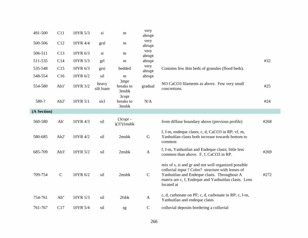
266
491-500 C11 10YR 5/3 si m very
abrupt
500-506 C12 10YR 4/4 grsl m very
abrupt
506-511 C13 10YR 6/3 si m very
abrupt
511-535 C14 10YR 5/3 grl m abrupt #32
535-548 C15 10YR 6/3 grsi bedded very
abrupt Contains few thin beds of granules (flood beds).
548-554 C16 10YR 6/2 sil m abrupt
554-580 Ab1' 10YR 3/2 heavy
silt loam
3mpr
breaks to
3msbk
gradual NO CaCO3 filaments as above. Few very small
concretions. #25
580-? Ab2' 10YR 5/1 sicl
3copr
breaks to
3msbk
N/A #24
(A Section)
560-580 Ab' 10YR 4/3 sil (3copr -
)(3?)1msbk from diffuse boundary above (previous profile) #268
580-685 Ab2' 10YR 4/2 sil 2msbk G
f, f-m, endeque clasts; c, d, CaCO3 in RP; vf, m,
Yanhuitlan clasts both increase towards bottom to
common
685-709 Ab3' 10YR 5/2 sil 2msbk A f, f-m, Yanhuitlan and Endeque clasts; little less
common than above. F, f, CaCO3 in RP. #269
709-754 C 10YR 6/2 sil 2msbk C
mix of s, si and gr and not well organized possible
colluvial input ? Color? structure with lenses of
Yanhuitlan and Endeque clasts. Throughout A
matrix are c, f, Endeque and Yanhuitlan clasts. Lens
located at
#272
754-761 Ab'' 10YR 5/3 sil 2fsbk A c, d, carbonate on PF; c, d, carbonate in RP; c, f-m,
Yanhuitlan and endeque clasts
761-767 C17 10YR 5/4 sil sg C colluvial deposits bordering a colluvial

267
767-783 C18 10YR 6/3 sil massive G
colluvial layer bordered by fluvial lens on bottom
with f, med Endeque clasts. F, f, Yanhuiltan clasts,
different from above and below by increaseing
Endeque and decreasing Yanuitlan clasts
783-788 C19 10YR 5/4 sil; f-cos,
fgr sg-massive C
c, f-m, Yanhuitlan clasts; f, f-m, Endeque clasts;
increase in Endeque clasts; fluvial fining upwards
sequences gr-si.
788-797 C20 darker layer with charcoal (ashy…?)
797-850 C21 10YR 4/4 lsi/ls-fgr laminated C
mainly a, vf-m Yanhuitlan clasts and f, f, Endeque
clasts in laminated planar and possibly cross trough
beds
850-897 C22 10YR 4/4 ls-cogr laminated
planar VA
different from abaove based on particle size. F, f-m
gr endeque clasts; a, f-vco Yanhuitlan clasts
897-913 C23 10YR 5/4 sil-s massive some laminated beds observable. Vf, f, Endeque
clasts; f, f-m, Yanhuitlan clasts
C24
(B Section)
897-937 C25 10YR 5/4 sil-fgr massive-sg VA
a, f-m, Yanhuitlan clasts (as gr and s); f, f-m,
Endeque clasts; same laminations in si-fs and s-gr
beds
#273
937-977 C26 10YR 4/3 sil-fgr massive C
f, f, laminated beds; a few gravel lenses; with
mainly Yanhuitlan and some Endeque clasts. Fining
up sequences
#271
977-1009 C27 10YR 6/3 sil-fgr 2mgr G f-c, f-m, Yanhuitlan and f, f, Endeque inclusions
1009-
1032 C28 10YR 5/3 si/sil
massive-
1fsbk C
c, d, CaCO3 in RP; original fining upward sequence
from s-gr below?
1032-
1056 C29 10YR 6/2 sil-fgr sg-1fgr A
majority endeque f-m gr clasts; f, f, Yanhuitlan
clasts
1056-
1122 C30 10YR 6/3 si-cos
massive/la
minated VA
similar to above, but no structure and smaller clasts;
c, f-m, endeque clasts
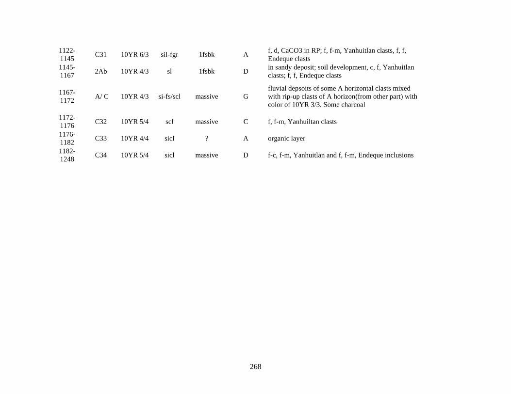
268
1122-
1145 C31 10YR 6/3 sil-fgr 1fsbk A
f, d, CaCO3 in RP; f, f-m, Yanhuitlan clasts, f, f,
Endeque clasts
1145-
1167 2Ab 10YR 4/3 sl 1fsbk D
in sandy deposit; soil development, c, f, Yanhuitlan
clasts; f, f, Endeque clasts
1167-
1172 A/ C 10YR 4/3 si-fs/scl massive G
fluvial depsoits of some A horizontal clasts mixed
with rip-up clasts of A horizon(from other part) with
color of 10YR 3/3. Some charcoal
1172-
1176 C32 10YR 5/4 scl massive C f, f-m, Yanhuiltan clasts
1176-
1182 C33 10YR 4/4 sicl ? A organic layer
1182-
1248 C34 10YR 5/4 sicl massive D f-c, f-m, Yanhuitlan and f, f-m, Endeque inclusions

269

270
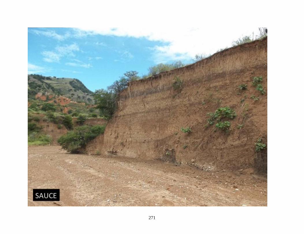
271

272
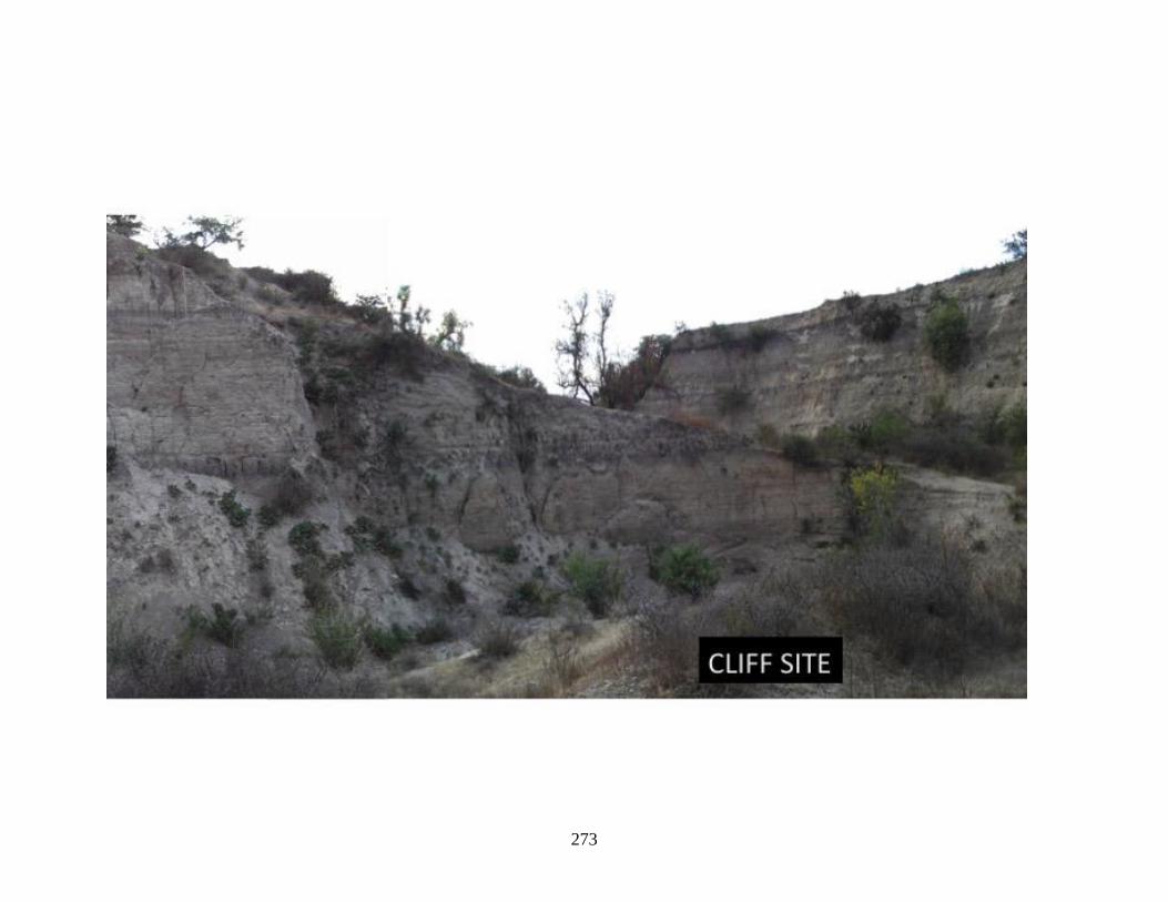
273
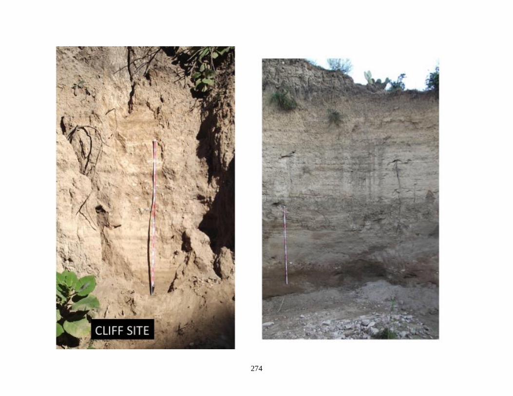
274

275

276

277

278

279

280
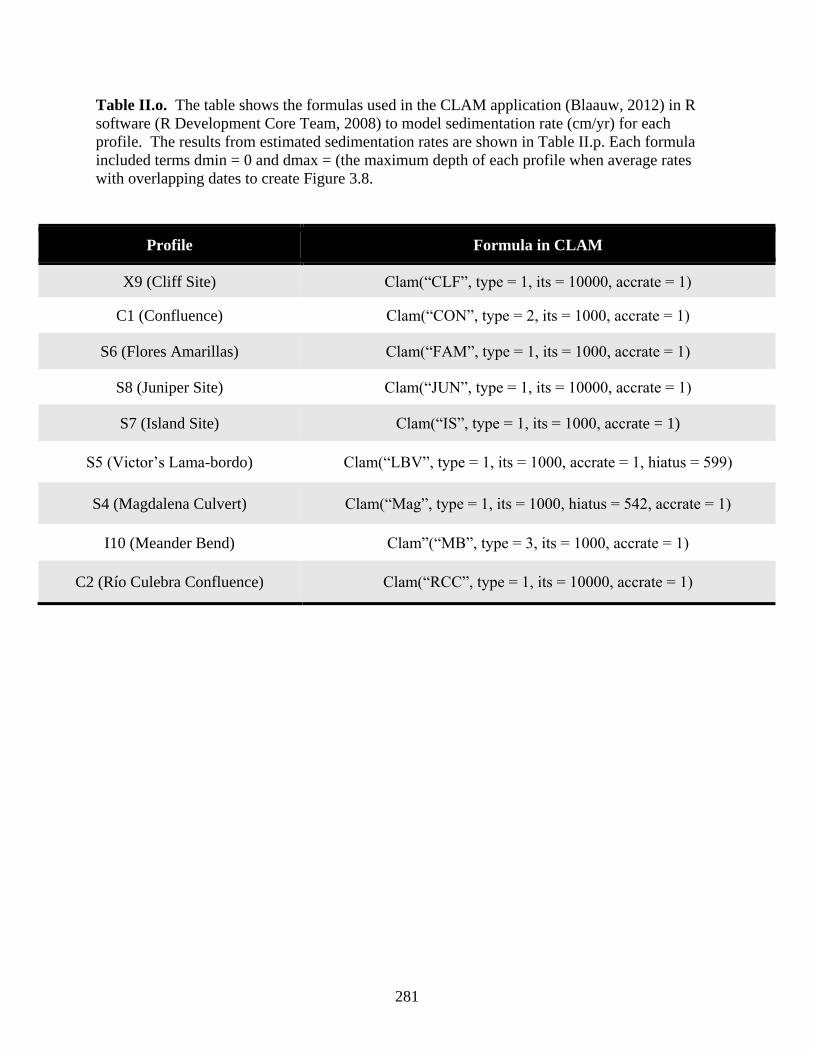
281
Table II.o. The table shows the formulas used in the CLAM application (Blaauw, 2012) in R
software (R Development Core Team, 2008) to model sedimentation rate (cm/yr) for each
profile. The results from estimated sedimentation rates are shown in Table II.p. Each formula
included terms dmin = 0 and dmax = (the maximum depth of each profile when average rates
with overlapping dates to create Figure 3.8.
Profile Formula in CLAM
X9 (Cliff Site) Clam(“CLF”, type = 1, its = 10000, accrate = 1)
C1 (Confluence) Clam(“CON”, type = 2, its = 1000, accrate = 1)
S6 (Flores Amarillas) Clam(“FAM”, type = 1, its = 1000, accrate = 1)
S8 (Juniper Site) Clam(“JUN”, type = 1, its = 10000, accrate = 1)
S7 (Island Site) Clam(“IS”, type = 1, its = 1000, accrate = 1)
S5 (Victor’s Lama-bordo) Clam(“LBV”, type = 1, its = 1000, accrate = 1, hiatus = 599)
S4 (Magdalena Culvert) Clam(“Mag”, type = 1, its = 1000, hiatus = 542, accrate = 1)
I10 (Meander Bend) Clam”(“MB”, type = 3, its = 1000, accrate = 1)
C2 (Río Culebra Confluence) Clam(“RCC”, type = 1, its = 10000, accrate = 1)

282
Table II.p. The table shows the results from estimated sedimentation rates using the formula
and procedures as described in Table II.o.. Only strata that did not contain any major hiatus or
well-developed paleosol formation (excluding cumulic paleosols), and which fell within two
radiocarbon ages (versus modeled ages).
Site ID Depth
(cm)
Age (Median
Cal BP)
Rate
(cm/yr)
S5 119 599 0.98
S5 127 607 0.98
I10 243 996 0.25
C3 767 1065 0.75
S7 137 1223 0.35
S7 280 1626 0.09
I10 470 1913 0.25
S7 330 2143 0.13
S7 351 2329 0.14
S5 191 2746 3.03
S7 522 3511 0.92
S5 1075 3604 4.55
S4 246 3834 0.28
S4 398 4360 0.63
X9 253 6375 0.06
C2 490 9063 0.14
X9 450 9629 0.4
X9 785 10474 0.55
X9 1749 12207* 0.55
X9 1750 12213** 0.14
X9 1799 12583 0.14
X9 1800 12581 0.19
C2 997 12710* 0.14
X9 2289 15201* 0.19
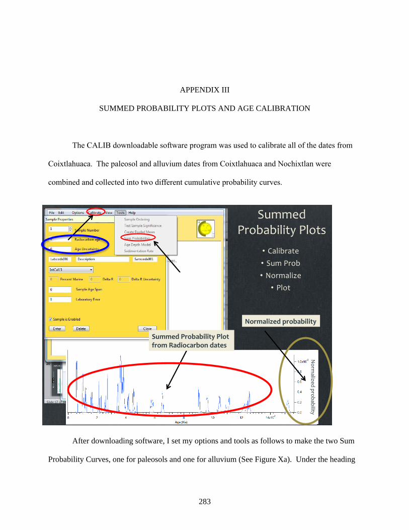
283
APPENDIX III
SUMMED PROBABILITY PLOTS AND AGE CALIBRATION
The CALIB downloadable software program was used to calibrate all of the dates from
Coixtlahuaca. The paleosol and alluvium dates from Coixtlahuaca and Nochixtlan were
combined and collected into two different cumulative probability curves.
After downloading software, I set my options and tools as follows to make the two Sum
Probability Curves, one for paleosols and one for alluvium (See Figure Xa). Under the heading
SummedProbabilityPlots
• Calibrate
• SumProb
• Normalize
• Plot
Norm
alize
dpro
bability
Normalizedprobability
SummedProbabilityPlotfromRadiocarbondates

284
CALIBRATION I defined how I wanted the calibration to be displayed. I checked the 1- and 2-
sigma precisions and calibration in years BP. I also checked “write distribution file”. Then,
under OPTIONS, I chose plot options, and selected Single Sample Cumulative Probability. I
also checked: “Make postscript Plot File”. Next, I clicked on File>Open> New. I entered in the
C-14 Radiocarbon age and the Age Uncertainty for the paleosols, changing the Labcode number
for each successive entry. After I entered all of the dates for the paleosols, I clicked on
CALIBRATE.
To obtain the Summed Probability values, I clicked on TOOLS>Summed Probabilities.
I opened each of the individual calibrated files and the summed probability files located in the
CALIB folder into wordpad, saved as text, and then imported these into EXCEL. I used the
same procedure to make a Sum Probability Curve for the alluvium. The Sum Probability Curves
were plotted in IGOR with the stable oxygen isotope data from the stalagmites from Guerrero
and qualitatively compared (see text for graphs).
In order to conduct the quantitative analysis, I edited the probability curve values in
Excel, so that they matched the dates and corresponding stable oxygen isotope values from the
stalagmites. For example, I only kept the dates and corresponding probability information from
the probability curves that were the same as the dates corresponding to the stalagmite isotope
values. The probability information from the cumulative curves was used to divide the paleosol
or alluvium dates into two further categories: either corresponding to a dated alluvium or
paleosol, or having a value of zero (i.e., no probability of being a date associated with either
one). The result were 2 pairs of data, each having a date and an isotope value, which
corresponded to one of the following 4 categories: isotope values corresponding to dated
paleosols (Category: Paleosol1), isotope information corresponding to dated alluvium Category:

285
Alluvium1), isotope values not corresponding to dated paleosols (Category: Paleosol0), and
isotope data not relating to dated alluvium (Category: Alluvium0). These categories were further
subdivided into those based on age (e.g., early vs. late Holocene) and on overarching climatic
phenomena (e.g., ENSO, North Atlantic). Any significant difference between categories was
detected by conducting t-tests and non-parametric tests (e.g., Mann-Whitney and Wilcoxon
tests). Since there were so few paleosol and no alluvium dates from the late Pleistocene, the
quantitative analysis only incorporated dates since the Terminal Pleistocene (in this study after
~16.0 cal ka BP). A similar procedure was used in filtering the sand data from el Junco, and the
Sum Probability Curves for alluvium and paleosols.
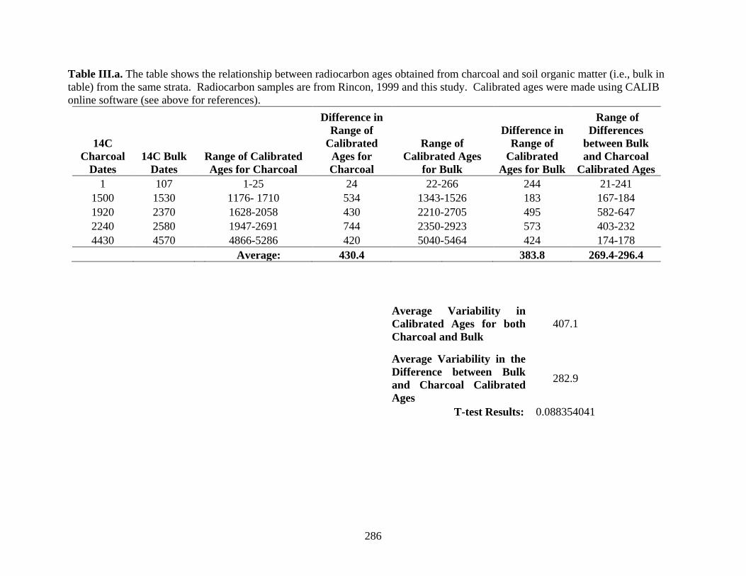
286
Table III.a. The table shows the relationship between radiocarbon ages obtained from charcoal and soil organic matter (i.e., bulk in
table) from the same strata. Radiocarbon samples are from Rincon, 1999 and this study. Calibrated ages were made using CALIB
online software (see above for references).
14C
Charcoal
Dates
14C Bulk
Dates
Range of Calibrated
Ages for Charcoal
Difference in
Range of
Calibrated
Ages for
Charcoal
Range of
Calibrated Ages
for Bulk
Difference in
Range of
Calibrated
Ages for Bulk
Range of
Differences
between Bulk
and Charcoal
Calibrated Ages
1 107 1-25 24 22-266 244 21-241
1500 1530 1176- 1710 534 1343-1526 183 167-184
1920 2370 1628-2058 430 2210-2705 495 582-647
2240 2580 1947-2691 744 2350-2923 573 403-232
4430 4570 4866-5286 420 5040-5464 424 174-178
Average: 430.4 383.8 269.4-296.4
Average Variability in
Calibrated Ages for both
Charcoal and Bulk
407.1
Average Variability in the
Difference between Bulk
and Charcoal Calibrated
Ages
282.9
T-test Results: 0.088354041