last name analysis of mobility, gender imbalance, and ... · and nepotism across academic systems...

Last name analysis of mobility, gender imbalance,and nepotism across academic systemsSupporting InformationJacopo Grillia and Stefano Allesinaa,b,c

aDepartment of Ecology & Evolution, University of Chicago, 1101 E. 57th Chicago, IL 60637, USA.; bComputation Institute, University of Chicago.; cNorthwestern Institute onComplex Systems, Northwestern University.

S1. Data

For our analysis, we collected a large database containing information on university professors working in Italy, France, and theUnited States of America.

Italy The data were downloaded from the website cercauniversita.cineca.it, maintained by the Italian Ministry of Education,University and Research, in September 2016. The website provides data on all Italian university professors from year 2000onward. For the years 2000, 2005, 2010, and 2015, we downloaded data on all the disciplinary fields (Area—a coarse-graineddivision into 14 fields). The number of professors in the database ranged from 52,004 (year 2000) to 60,288 (year 2010). Datainclude the first and last name, the institution, information on the disciplinary field, rank, and gender of all Italian professors.We enriched the data by adding a region and city to every institution. In case of institutions with multiple campuses, wechose the main one. All names were transliterated into ASCII, and made into lowercase, for better handling of accents andapostrophes. Finally, we numbered all last names and first names, and used this anonymized version of the data for our analysis(the same was done for all data sets).

The labels in the figures and tables refer to the following disciplinary fields (Area): Agr, agriculture and veterinary sciences(07 Scienze agrarie e veterinarie); Bio, biological sciences (05 Scienze biologiche); Chem, chemistry and pharmaceutical sciences(03 Scienze chimiche); CivEng, civil engineering and architecture (08 Ingegneria civile e architettura); Econ, economics andstatistics (13 Scienze economiche e statistiche); Geo, geology and Earth sciences (04 Scienze della terra); Hum, philology,literature, archeology (10 Scienze dell’antichità, filologico-letterarie e storico artistiche); IndEng, industrial, electronic, andelectric engineering (09 Ingegneria industriale e dell’informazione); Law, law (12 Scienze giuridiche); Math, mathematicsand computer science (01 Scienze matematiche e informatiche); Med, medical sciences (06 Scienze mediche); Ped, pedagogy,psychology, history, philosophy (11 Scienze storiche, filosofiche, pedagogiche, psicologiche); Phys, physics and astrophysics (02Scienze fisiche); Soc, social and political sciences (14 Scienze politiche e sociali).

France The data were downloaded from the official website of the CNRS web-ast.dsi.cnrs.fr/l3c/owa/annuaire.recherchein September 2016. Queries targeted each and every one of the research units (by specifying a Code unité). The list of personnelof each of the Unité mixte de recherche and Unité propre de recherche was downloaded. Units operating principally outside ofcontinental France and Corse were excluded (e.g., units working in Martinique and Guyane). For each unit, we assigned a fieldby selecting the most represented Groupe(s) de discipline. For example, a unit listing SC - Chimie (70%) and SDE - Sciences del’Environnement (30%) would be assigned to Chemistry. In case of ties, we pick the first listed field. Similarly, for assigning theregion and city to each unit, in case of multiple listings we chose the first city and region. Among the personnel, we extractedthe names of all Chercheurs CNRS as well as Chercheurs non CNRS (i.e., researchers working in a CNRS laboratory, butofficially affiliated with another research institution). Last names are listed in all capitals, while first name(s) are capitalized.We separated the two using regular expressions, and transliterated the strings to ASCII. Maiden names were gathered bymatching the records with those obtained searching the website annuaire.cnrs.fr/l3c/owa/personnel.frame_recherche.

The labels in the figures refer to the following disciplinary fields (Groupe de discipline): Math, Mathematics (MATHMathématiques); Phys, Physics (PHY Physique); HE Phys, High Energy Physics (PNHE - Physique Nucléaire et des HautesEnergies); Chem, Chemistry (SC - Chimie); Env, Environmental Sciences (SDE - Sciences de l’Environnement); Cell, Cell andMolecular Biology (SDV1 - Biologie cellulaire et moléculaire); Neuro, Neuroscience (SDV2 - Biologie intégrative et neurosciences);Genet, Genetics (SDV3 - Génétique); Hum, Humanities and Social Sciences (SHS - Sciences de l’Homme et de la Société); Eng,Engineering (SPI - Sciences pour l’Ingénieur); Geo, Earth Science and Astronomy (SPU - Sciences de la Planète et Univers);Info, Information and Communications Sciences (STIC - Sciences et Technologies de l’Information et de la Communication).

United States For institutions in the US, a ready-made database of all professors does not exist. We therefore took a differentroute, and downloaded data on public salaries. Many states list the salaries of all the state employees, often includinguniversity personnel. We searched for this type of data, privileging the states in which more than one R1 operates (to havemultiple institutions within a region/state). Table S1 lists the institutions, state, and website from which the information wasdownloaded. For each institution, we downloaded the most recent year available (typically, 2015).

1

State Institution(s) Website(s)

CaliforniaUC Berkeley; UC Davis; UC Irvine; UC LosAngeles; UC Riverside; UC San Diego; UCSanta Barbara; UC Santa Cruz

ucannualwage.ucop.edu

Florida F International U; F State U; U Central F; UF floridahasarighttoknow.myflorida.com

GeorgiaG Institute Technology; G State U; UGAthens

open.georgia.gov/sta/search.aud

Illinois UI Chicago; UI Urbana-Champaign salarysearch.ibhe.org/search.aspx

Michigan M State U; UM Ann Arbor; Wayne State Uwww.msusalaries.info (M State U); www.umsalary.info(UM Ann Arbor); www.waynestatesalaries.info (WayneState U)

New YorkCity U NY; State U NY (SUNY) Albany;SUNY Buffalo State College; SUNY StonyBrook

seethroughny.net/payrolls

North Carolina NC State U; UNC Chapel Hillwww.newsobserver.com/news/databases/public-salaries/

TexasT A & M U; U Houston; U North T; UTArlington; UT Austin; UT Dallas

salaries.texastribune.org/agencies/university

Washington UW; W State U fiscal.wa.gov/WaStEmployeeHistSalary.txtWisconsin UW Madison; UW Milwaukee host.madison.com/ (search for University Salaries)

Table S1. List of US R1 Public Universities considered in this study, along of the website from which the list of professors was downloaded.

We then filtered all the data in order to select only Assistant, Associate or Full professors. Adjunct and Visiting professors,as well as research assistants and associates were removed. Note that, contrary to the case of Italy and France, the data doesnot contain a disciplinary field. We therefore attempted matching researchers and fields by searching for their last name, firstname (and when available, middle initials or middle name) in Scopus. For each researcher, a pairing was considered valid if itmatched the institution, the last name, and the first name (initials were also matched when available).

For each researcher, Scopus returns the number of articles published in a given “subject-area”. We took the most representedsubject-area for each researcher and coarse grained into the 12 labels displayed in the figures and tables. In particular, themapping between the Scopus subject-areas∗ and our labels is as follows: Agr, AGRI; Bio, BIOC, ENVI, MULT, NEUR; Chem,CENG, CHEM, ENER; Econ, BUSI, DECI, ECON; Geo, EART; Hum, ARTS; IndEng, ENGI; Math, COMP, MATH; Med, DENT,HEAL, IMMU, MEDI, NURS, PHAR; Ped, PSYC; Phys, MATE, PHYS; Soc, SOCI.

Data availability All the data are available at http://github.com/StefanoAllesina/namepairs for download in anonymizedform: the first and last names have been replaced with numerical identifiers. All the analysis presented in this study have beenperformed on this database.

S2. Isonymous pairs

As explained in the main text, throughout the article we use the number of isonymous pairs (IPs) as our main observable.For a given institution and scientific field, we take the department to be the set of professors working in that institution andfield. For a department d, the number of professors having last name i is nid. The number of isonymous pairs is thereforepd =

∑i

(nid

2

). This quantity can be interpreted as the number of edges in a graph in which the nodes are the researchers

working in the department, and edges connect researchers with the same last name (Figure S1).We chose this observable because it has excellent statistical properties. In particular, take a list of names (for example, all

the researchers working in Sardinia), and randomly extract a sample of k researchers without replacement. Then, the expectednumber of IPs in the set is approximately p

(k2

), where p is the proportion of isonymous pairs in the list of names:

p =∑

i

(ni2

)(∑ini

2

) =∑

ini(ni − 1)(∑

jnj

)(∑jnj − 1

) [S1]

Figure S2 shows that the variance around this expectation is very modest, guaranteeing that we can detect small butsignificant deviations, and that the number of IPs has better statistical properties than other measures—for example thenumber of unique last names in the sample. The choice of measuring IPs in this way differentiates our work from previousattempts at measuring the level of familism in academia. For example, Allesina (1) counted the number of distinct namesin each discipline, while Durante et al. (2) constructed two indices of “homonymy” by counting how many members of adepartment have one (or more) namesakes as colleagues.

∗For a list of all subject-areas, see api.elsevier.com/documentation/search/SCOPUSSearchTips.htm.

PNAS | 2 Grilli et al.

Fig. S1. Number of isonymous pairs as the number of edges in a graph. We can take all the researches in a department (left, University of Bari, Economics, 2005; right,Michigan State University, Industrial Engineering), and connect any two researchers that have the same last name. The total number of edges in the graph is the number of IPs,pd. In the figure, researchers with unique last names are colored in gray.

Fig. S2. Statistical properties of IPs. We took two data sets: the researchers working in Sardegna in 2000 (1580 researchers) and the mathematicians working at the US publicinstitutions we included in the analysis (3259 people). For each sample size k (from 50 to 1500 in steps of 50), we sampled k researchers at random and computed the numberof IPs (red), or the number of unique last names in the sample (blue). We repeated the sampling 100 times for each value of k and data set (the error bars mark the 5th and95th percentile of the distribution). The black line shows the expectation: while the number of IPs scales with

(k2

), the number of unique last names in the sample scales in a

non-trivial, non-linear way with k.

Grilli et al. PNAS | 3

S3. Geographical distance and similarity

As discussed in the main text, Fig. 1 suggests the existence of a clustering by city of Italian last names, which is instead notpresent for US institutions. In this section, we quantify the similarity between the last names distribution of two cities andcorrelate this quantity with their geographical distance. The results support the conclusion of the main text, showing that thesimilarity between the last names of two Italian cities is generally negatively correlated with distance and that this pattern isnot present for cities in the US.

Let nic be the number of people with last name i in city c and nc =∑

inic the number of people in city c. The fraction of

people with last name i in city c is then π(c)i defined as

π(c)i = nic

nc. [S2]

We define the similarity between city c and city c′ as

Sc|c′ =∑

iπ

(c)i π

(c′)i∑

i

(π

(c′)i

)2 . [S3]

This choice is motivated as follows. The numerator is (proportional to) the covariance between π(c)i and π(c′)

i . The covariancebetween these frequency has been used, under the name of kinship, to compare last names of different locations (3). Thecovariance is, on the other hand, strongly influenced by the sample size of the two different cities. Our strategy is to normalizethe covariance to obtain a quantity Sc|c′ that is independent of the sample size of city c′.

Assuming that the last names of city c were sampled from the same distribution of city c′, one would expect to have,on average under this null hypothesis, nic = ncπ

(c′)i . The expected value of the covariance is therefore (proportional to)∑

i

(π

(c′)i

)2. Dividing the covariance by its expected values under the null hypothesis, one obtains Eq. S3. Under this definition,

the similarity Sc|c′ is not symmetric and does not depend on the sample size of city c′ (while it depends on the size of city c).Figures S3, S4 and S5 show, for each city c, the similarity between c and another city c′ vs. the distance between c and c′.

Italian last names S3 are characterized by a strong geographical pattern. For many cities, the similarity clearly decreaseswith distance, indicating a geographical signal of last names in the Italian universities. In France and in the US this pattern isnot present. This could be caused by different factors. One possibility is that the typical length-scale of spatial correlation oflast names is smaller than the resolution at which we are observing the system. Alternatively, the last names of the wholepopulation could lack a geographical signal (i.e., names are not associated to a specific geographical location). Finally, theabsence of a relation between similarity and distance could indicate that the university system is effectively well-mixed andresearcher move within the nation (or that their movement is not determined by geographical distance from their place ofbirth). Immigration from abroad does also play an important role in reducing the geographical signal.

S4. Last names by region and sector

Tables S2, S3 report the results for the three randomizations when summing IPs by field or by region for the Italian data set(2015). Tables S4 and S5 for the CNRS data, and Tables S7 and S6 for the US institutions. The tables correspond to Figures1 and 2 in the main text.

field observed by country by city by fieldAgr 86 27.5 (5.8) p < 0.001 66.8 (9.7) p = 0.033 26.1 (5) p < 0.001Bio 125 42 (7.2) p < 0.001 100.2 (11.8) p = 0.025 43.4 (6.8) p < 0.001

Chem 70 17 (4.4) p < 0.001 43.4 (7.4) p = 0.001 17.3 (4.2) p < 0.001CivEng 104 35.5 (7) p < 0.001 73.7 (11.3) p = 0.011 38.7 (6.6) p < 0.001Econ 91 34.5 (6.5) p < 0.001 70.7 (9.7) p = 0.026 36.8 (6.2) p < 0.001Geo 5 2.2 (1.5) p = 0.075 5.3 (2.4) p = 0.596 2 (1.4) p = 0.054Hum 61 41.4 (7.2) p = 0.007 87.7 (10.6) p = 0.997 34.9 (5.9) p < 0.001

IndEng 205 78.4 (10.9) p < 0.001 153.4 (17.1) p = 0.005 83.8 (10) p < 0.001Law 102 31.1 (6) p < 0.001 76.6 (9.8) p = 0.009 34.2 (5.9) p < 0.001Math 46 17.4 (4.5) p < 0.001 37.6 (6.8) p = 0.125 18.2 (4.3) p < 0.001Med 579 232.9 (20.5) p < 0.001 467.7 (28.8) p < 0.001 249.9 (17.7) p < 0.001Ped 75 34.9 (6.6) p < 0.001 73.3 (9.7) p = 0.437 36.1 (6.2) p < 0.001Phys 25 9.2 (3.2) p < 0.001 20.5 (4.9) p = 0.201 9.1 (3) p < 0.001Soc 12 5.3 (2.4) p = 0.013 11.3 (3.6) p = 0.447 6 (2.5) p = 0.024

Table S2. Observed and expected number of IPs for the dataset Italy, 2015. For each field, we report the observed number of pairs, as wellas the expectation when randomizing last names either within academic system (by country), within regions (by region), etc. The number inparenthesis is the standard deviation. In bold values that have a p−value ≤ 0.05/number of tests.


Bari Bologna Cagliari Caserta Catania

Crotone Firenze Genova Messina Milano

Napoli Padova Palermo Parma Pavia

Perugia Pisa Roma Salerno Torino

0.1

1.0

0.1

1.0

0.01

0.10

1.00

0.1

1.0

0.1

1.0

0.1

1.0

0.1

1.0

0.1

1.0

0.1

1.0 1

0.1

1.0

0.1

1.0

0.1

1.0

0.1

1.0

0.1

1.0

0.1

1.0

0.1

1.0 1

0.1

1.0

0.1

1.0

0 250 500 750 0 200 400 600 800 0 200 400 600 800 0 200 400 600 0 300 600 900

0 250 500 750 1000 0 200 400 600 800 0 250 500 750 0 250 500 750 1000 0 250 500 750 1000

0 200 400 600 0 250 500 750 0 250 500 750 0 250 500 750 0 250 500 750 1000

0 200 400 600 0 200 400 600 800 0 200 400 0 200 400 600 0 250 500 750 1000distance [km]

Nam

e si

mila

rity

Fig. S3. Correlation between similarity of the last names of two cities and their geographical distance for the 20 cities in Italy with the largest number of researchers. Eachfigure shows the similarity Sc|c′ , as defined in Eq. S3, between a city c (indicated in the title of the panel) and all the other cities c′ vs the geographical distance between c andc′. Each city c is compared only to cities c′ with more than 50 researchers. The blue line is the best fitting spline, once removed the point at distance 0 (corresponding to Sc|c,which is equal to 1 by definition).


Aix en provence Dijon Gif sur yvette Grenoble Lyon

Marseille Montpellier Nantes Nice Orsay

Palaiseau Paris Pessac Rennes Strasbourg

Talence Toulouse Vandoeuvre les nancy Villeneuve d ascq Villeurbanne

0.01

0.10

1.00

0.1

1.0

0.1

1.0

0.1

1.0

0.1

1.0

0.1

1.0

0.1

1.0

0.1

1.0

0.01

0.10

1.00

0.01

0.10

1.00

0.01

0.10

1.00 1

0.01

0.10

1.00

0.1

1.0

0.1

1.0

0.01

0.10

1.00

0.1

1.0

0.1

1.0

0.01

0.10

1.00

0.1

1.0

0 250 500 750 0 200 400 600 0 250 500 750 0 250 500 750 0 200 400 600 800

0 250 500 750 1000 0 200 400 600 800 0 250 500 750 1000 0 250 500 750 1000 0 250 500 750

0 250 500 750 0 250 500 750 0 200 400 600 800 0 300 600 900 0 250 500 750

0 200 400 600 800 0 200 400 600 800 0 200 400 600 800 0 250 500 750 1000 0 200 400 600 800distance [km]

Nam

e si

mila

rity

Fig. S4. Same as Figure S3, for the 20 cities in France with the largest number of researchers.

Ann Arbor MI Athens GA Atlanta GA Austin TX Berkeley CA

Buffalo NY Champaign IL Chapel Hill NC Chicago IL College Station TX

Davis CA East Lansing MI Gainesville FL Houston TX Irvine CA

Los Angeles CA Madison WI Raleigh NC San Diego CA Seattle WA

0.1

1.0

0.1

1.0

0.1

1.0

0.1

1.0

0.1

1.0

0.1

1.0

0.1

1.0

0.1

1.0

0.1

1.0

0.1

1.0

0.1

1.0

0.1

1.0

0.1

1.0

0.1

1.0

0.1

1.0

0.1

1.0

0.1

1.0

0.1

1.0

0.1

1.0

0.1

1.0

0 1000 2000 3000 0 1000 2000 3000 0 1000 2000 3000 0 1000 2000 0 1000 2000 3000 4000

0 1000 2000 3000 0 1000 2000 3000 0 1000 2000 3000 4000 0 1000 2000 3000 0 1000 2000 3000

0 1000 2000 3000 4000 0 1000 2000 3000 0 1000 2000 3000 4000 0 1000 2000 3000 0 1000 2000 3000 4000

0 1000 2000 3000 4000 0 1000 2000 0 1000 2000 3000 4000 0 1000 2000 3000 4000 0 1000 2000 3000 4000distance [km]

Nam

e si

mila

rity

Fig. S5. Same as Figure S3, for the 20 cities in the US with the largest number of researchers.


region observed by country by city by fieldAbruzzo 21 7.3 (2.9) p < 0.001 14.7 (3.6) p = 0.062 7.6 (2.9) p < 0.001

Basilicata 4 0.8 (0.9) p = 0.011 1.8 (1.3) p = 0.1 0.8 (0.9) p = 0.01Calabria 33 6.2 (2.6) p < 0.001 31.9 (5.4) p = 0.444 6.4 (2.7) p < 0.001

Campania 241 53.8 (8.4) p < 0.001 177.3 (14.1) p < 0.001 56.3 (8.5) p < 0.001Emilia-Romagna 138 56.6 (8.6) p < 0.001 112.1 (10.4) p = 0.009 58.3 (8.6) p < 0.001

Friuli-Venezia Giulia 7 5.6 (2.5) p = 0.334 5.5 (2.3) p = 0.309 5.7 (2.5) p = 0.343Lazio 209 148.9 (17.3) p = 0.002 180.8 (16.4) p = 0.052 157.1 (16.7) p = 0.003

Liguria 27 11.6 (3.8) p < 0.001 26.1 (5.1) p = 0.447 12.1 (3.8) p = 0.001Lombardia 244 120.9 (13.5) p < 0.001 211.7 (17.7) p = 0.043 127.7 (13.6) p < 0.001

Marche 13 5.2 (2.4) p = 0.005 11.3 (3.1) p = 0.334 5.4 (2.4) p = 0.006Molise 1 0.5 (0.7) p = 0.407 1 (1) p = 0.664 0.5 (0.8) p = 0.418

Piemonte 69 43.6 (7.8) p = 0.003 56.8 (7.5) p = 0.063 45.4 (7.9) p = 0.005Puglia 82 22.1 (5.2) p < 0.001 55.4 (7.2) p < 0.001 22.8 (5.2) p < 0.001

Sardegna 99 9.2 (3.2) p < 0.001 83.6 (9.1) p = 0.056 9.4 (3.2) p < 0.001Sicilia 236 37 (6.8) p < 0.001 181.4 (13.5) p < 0.001 38.7 (6.9) p < 0.001

Toscana 79 33.5 (6.4) p < 0.001 62.5 (7.8) p = 0.024 34.6 (6.4) p < 0.001Trentino-Alto Adige 4 2.6 (1.7) p = 0.261 3.1 (1.7) p = 0.37 2.7 (1.7) p = 0.285

Umbria 26 7.7 (3) p < 0.001 16.7 (4) p = 0.02 7.9 (3) p < 0.001Valle D’Aosta 0 0 (0.2) p = 1 0 (0) − 0 (0.2) p = 1

Veneto 53 36.3 (6.8) p = 0.014 54.4 (7.2) p = 0.595 37.3 (6.8) p = 0.019Table S3. Observed and expected number of IPs for the dataset Italy, 2015. For each region, we report the observed number of pairs, as wellas the expectation when randomizing last names either within academic system (by country), within regions (by region), etc. The number inparenthesis is the standard deviation. In bold values that have a p−value ≤ 0.05/number of tests.

field observed by country by city by fieldCell 13 8.1 (3) p = 0.082 10.3 (3.4) p = 0.244 7.7 (2.8) p = 0.054

Chem 31 15.4 (4.1) p < 0.001 24.2 (4.9) p = 0.104 18.2 (4.3) p = 0.005Eng 27 10.3 (3.4) p < 0.001 22.8 (4) p = 0.172 11.8 (3.5) p < 0.001Env 16 6.9 (2.7) p = 0.004 9.5 (3) p = 0.031 9.4 (3.1) p = 0.031

Genet 7 4.5 (2.3) p = 0.185 5.3 (2.4) p = 0.281 4.4 (2.1) p = 0.153Geo 13 7.7 (2.9) p = 0.058 9.1 (3.2) p = 0.139 8.1 (2.8) p = 0.069

HE Phys 1 1.8 (1.4) p = 0.82 1.8 (1.4) p = 0.824 1.5 (1.2) p = 0.791Hum 56 27.3 (5.4) p < 0.001 40.7 (6.2) p = 0.012 28.3 (5.4) p < 0.001Info 73 42.6 (7.1) p < 0.001 60.4 (7.9) p = 0.066 42.1 (6.5) p < 0.001

Math 32 16.6 (4.4) p = 0.002 21.4 (5.1) p = 0.031 15.9 (4) p < 0.001Neuro 10 5.8 (2.5) p = 0.08 7.1 (2.7) p = 0.178 6 (2.4) p = 0.084Phys 15 8.4 (3.1) p = 0.033 10.4 (3.4) p = 0.12 7.7 (2.8) p = 0.014

Table S4. Observed and expected number of IPs for the dataset France CNRS using maiden names, 2016. For each field, we report theobserved number of pairs, as well as the expectation when randomizing last names either within academic system (by country), withinregions (by region), etc. The number in parenthesis is the standard deviation. In bold values that have a p−value ≤ 0.05/number of tests.


region observed by country by city by fieldAlsace 16 6.5 (2.8) p = 0.004 12.2 (3.1) p = 0.142 6.7 (2.8) p = 0.004

Aquitaine 9 6.9 (2.8) p = 0.267 8.1 (2.6) p = 0.414 7.2 (2.8) p = 0.303Auvergne 4 2.5 (1.7) p = 0.238 2.9 (1.5) p = 0.323 2.6 (1.7) p = 0.253

Basse-Normandie 2 1 (1) p = 0.265 2.1 (1.4) p = 0.633 1 (1) p = 0.267Bourgogne 2 1.7 (1.4) p = 0.507 2.2 (1.4) p = 0.667 1.9 (1.4) p = 0.552Bretagne 32 12.5 (3.9) p < 0.001 26.4 (4.8) p = 0.142 12.9 (3.9) p < 0.001Centre 1 1.6 (1.3) p = 0.787 1.4 (1.1) p = 0.786 1.6 (1.3) p = 0.798

Champagne-Ardenne 1 0.8 (1) p = 0.553 0.4 (0.5) p = 0.355 0.8 (1) p = 0.556Corse 11 0.5 (0.8) p < 0.001 7 (1.9) p = 0.031 0.6 (0.8) p < 0.001

Franche-Comté 8 2.9 (1.9) p = 0.022 5.6 (2) p = 0.177 3.1 (1.9) p = 0.024Haute-Normandie 2 0.7 (0.9) p = 0.152 1.4 (1) p = 0.436 0.8 (0.9) p = 0.171

Ile-de-France 51 40 (6.6) p = 0.062 41.8 (6.1) p = 0.082 40.9 (6.7) p = 0.078Languedoc-Roussillon 15 7.5 (2.9) p = 0.015 11 (3) p = 0.122 8.2 (3) p = 0.029

Limousin 3 1.9 (1.5) p = 0.283 3.2 (1.2) p = 0.715 1.9 (1.5) p = 0.29Lorraine 10 6.2 (2.7) p = 0.11 9.3 (2.8) p = 0.45 6.6 (2.7) p = 0.14

Midi-Pyrénées 23 13.9 (4) p = 0.025 17.3 (4.2) p = 0.109 14.2 (4) p = 0.029Nord-Pas-de-Calais 15 8.4 (3.1) p = 0.037 11.6 (3.1) p = 0.174 8.6 (3.1) p = 0.04

PaysdelaLoire 3 3.3 (1.9) p = 0.637 3.6 (1.8) p = 0.72 3.6 (2) p = 0.692Picardie 0 0.6 (0.8) p = 1 0.6 (0.7) p = 1 0.6 (0.8) p = 1

Poitou-Charentes 11 3.1 (1.9) p = 0.002 11 (2) p = 0.598 3.6 (2.1) p = 0.005Provence-Alpes-Côted’Azur 31 11.8 (3.6) p < 0.001 16.6 (3.9) p = 0.001 12.3 (3.6) p < 0.001

Rhône-Alpes 44 21.2 (4.9) p < 0.001 27.3 (5) p = 0.001 21.5 (4.9) p < 0.001Table S5. Observed and expected number of IPs for the dataset France CNRS using maiden names, 2016. For each region, we report theobserved number of pairs, as well as the expectation when randomizing last names either within academic system (by country), withinregions (by region), etc. The number in parenthesis is the standard deviation. In bold values that have a p−value ≤ 0.05/number of tests.

field observed by country by city by fieldAgr 35 33.8 (7.3) p = 0.434 35.2 (7.1) p = 0.519 37.4 (6.3) p = 0.663Bio 279 215.6 (21.1) p = 0.003 222 (20.2) p = 0.005 258.4 (18.3) p = 0.137

Chem 17 11.1 (3.7) p = 0.079 12.3 (3.9) p = 0.14 20.5 (4.6) p = 0.805Econ 40 26.9 (6) p = 0.025 33.2 (6.7) p = 0.174 32.1 (5.7) p = 0.1Geo 9 5.5 (2.6) p = 0.128 6.2 (2.7) p = 0.189 5.7 (2.4) p = 0.124Hum 44 58.6 (9.3) p = 0.956 62.2 (9.3) p = 0.984 41.2 (6.5) p = 0.346

IndEng 40 25.8 (5.9) p = 0.018 29.6 (6.4) p = 0.067 48.6 (7.4) p = 0.897Math 124 61.5 (9.5) p < 0.001 70.5 (10.2) p < 0.001 103.8 (10.6) p = 0.038Med 634 589.9 (43.3) p = 0.157 597 (37.5) p = 0.165 507.7 (28) p < 0.001Ped 29 10.2 (3.5) p < 0.001 11.8 (3.8) p < 0.001 9.3 (3) p < 0.001Phys 64 26 (5.9) p < 0.001 29 (6.2) p < 0.001 53.6 (7.5) p = 0.097Soc 164 150.1 (15.9) p = 0.196 169.8 (16.7) p = 0.638 129.8 (11.6) p = 0.003

Table S6. Observed and expected number of IPs for the dataset US public research institutions, 2016. For each field, we report the observednumber of pairs, as well as the expectation when randomizing last names either within academic system (by country), within regions (byregion), etc. The number in parenthesis is the standard deviation. In bold values that have a p−value ≤ 0.05/number of tests.

region observed by country by city by fieldCalifornia 203 176.2 (18.3) p = 0.08 167.1 (13.4) p = 0.006 178.4 (17.6) p = 0.089

Florida 199 183.8 (23.7) p = 0.255 183.5 (15.5) p = 0.164 184.1 (22.1) p = 0.245Georgia 86 53.5 (9.3) p = 0.001 67.4 (8.2) p = 0.018 60.7 (10.3) p = 0.014Illinois 104 82.6 (14) p = 0.075 86.3 (10.3) p = 0.055 84.2 (13.3) p = 0.08

Kansas 16 11.3 (3.9) p = 0.14 11.3 (3.2) p = 0.102 12.8 (4.2) p = 0.245Michigan 137 112.8 (14.6) p = 0.059 133.3 (12.6) p = 0.387 121.3 (15.1) p = 0.157New York 77 56.1 (9.4) p = 0.022 67.3 (8.4) p = 0.136 58.4 (9.6) p = 0.037

North Carolina 173 154.9 (21.9) p = 0.201 146.6 (14.8) p = 0.048 154.4 (20.1) p = 0.178Texas 161 104 (12.9) p < 0.001 132.4 (11.4) p = 0.009 120.7 (14.4) p = 0.005

Washington 250 200.1 (28.1) p = 0.049 224.1 (20) p = 0.105 193 (24.8) p = 0.019Wisconsin 73 79.5 (13.4) p = 0.684 59.8 (7.9) p = 0.06 80 (13.1) p = 0.705

Table S7. Observed and expected number of IPs for the dataset US public research institutions, 2016. For each region, we report the observednumber of pairs, as well as the expectation when randomizing last names either within academic system (by country), within regions (byregion), etc. The number in parenthesis is the standard deviation. In bold values that have a p−value ≤ 0.05/number of tests.


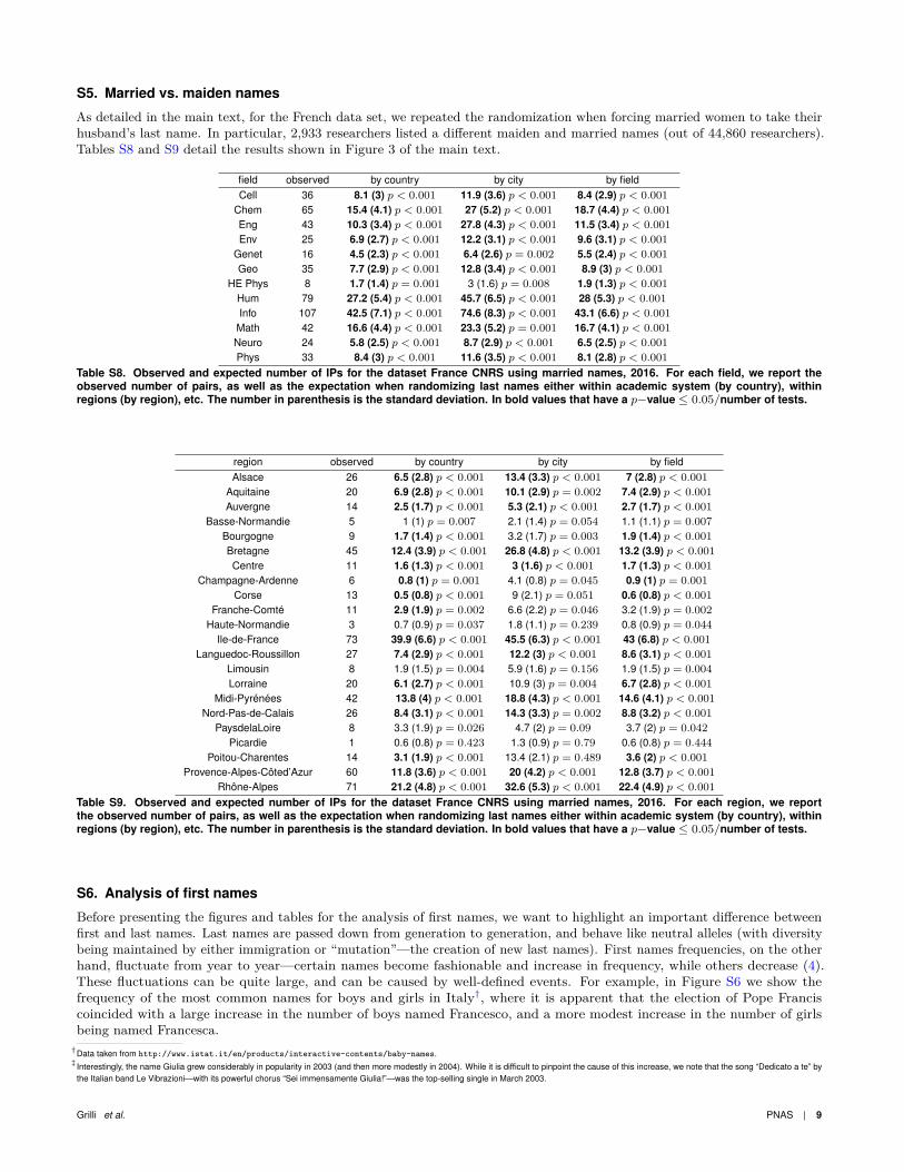
S5. Married vs. maiden names

As detailed in the main text, for the French data set, we repeated the randomization when forcing married women to take theirhusband’s last name. In particular, 2,933 researchers listed a different maiden and married names (out of 44,860 researchers).Tables S8 and S9 detail the results shown in Figure 3 of the main text.

field observed by country by city by fieldCell 36 8.1 (3) p < 0.001 11.9 (3.6) p < 0.001 8.4 (2.9) p < 0.001

Chem 65 15.4 (4.1) p < 0.001 27 (5.2) p < 0.001 18.7 (4.4) p < 0.001Eng 43 10.3 (3.4) p < 0.001 27.8 (4.3) p < 0.001 11.5 (3.4) p < 0.001Env 25 6.9 (2.7) p < 0.001 12.2 (3.1) p < 0.001 9.6 (3.1) p < 0.001

Genet 16 4.5 (2.3) p < 0.001 6.4 (2.6) p = 0.002 5.5 (2.4) p < 0.001Geo 35 7.7 (2.9) p < 0.001 12.8 (3.4) p < 0.001 8.9 (3) p < 0.001

HE Phys 8 1.7 (1.4) p = 0.001 3 (1.6) p = 0.008 1.9 (1.3) p < 0.001Hum 79 27.2 (5.4) p < 0.001 45.7 (6.5) p < 0.001 28 (5.3) p < 0.001Info 107 42.5 (7.1) p < 0.001 74.6 (8.3) p < 0.001 43.1 (6.6) p < 0.001

Math 42 16.6 (4.4) p < 0.001 23.3 (5.2) p = 0.001 16.7 (4.1) p < 0.001Neuro 24 5.8 (2.5) p < 0.001 8.7 (2.9) p < 0.001 6.5 (2.5) p < 0.001Phys 33 8.4 (3) p < 0.001 11.6 (3.5) p < 0.001 8.1 (2.8) p < 0.001

Table S8. Observed and expected number of IPs for the dataset France CNRS using married names, 2016. For each field, we report theobserved number of pairs, as well as the expectation when randomizing last names either within academic system (by country), withinregions (by region), etc. The number in parenthesis is the standard deviation. In bold values that have a p−value ≤ 0.05/number of tests.

region observed by country by city by fieldAlsace 26 6.5 (2.8) p < 0.001 13.4 (3.3) p < 0.001 7 (2.8) p < 0.001

Aquitaine 20 6.9 (2.8) p < 0.001 10.1 (2.9) p = 0.002 7.4 (2.9) p < 0.001Auvergne 14 2.5 (1.7) p < 0.001 5.3 (2.1) p < 0.001 2.7 (1.7) p < 0.001

Basse-Normandie 5 1 (1) p = 0.007 2.1 (1.4) p = 0.054 1.1 (1.1) p = 0.007Bourgogne 9 1.7 (1.4) p < 0.001 3.2 (1.7) p = 0.003 1.9 (1.4) p < 0.001Bretagne 45 12.4 (3.9) p < 0.001 26.8 (4.8) p < 0.001 13.2 (3.9) p < 0.001Centre 11 1.6 (1.3) p < 0.001 3 (1.6) p < 0.001 1.7 (1.3) p < 0.001

Champagne-Ardenne 6 0.8 (1) p = 0.001 4.1 (0.8) p = 0.045 0.9 (1) p = 0.001Corse 13 0.5 (0.8) p < 0.001 9 (2.1) p = 0.051 0.6 (0.8) p < 0.001

Franche-Comté 11 2.9 (1.9) p = 0.002 6.6 (2.2) p = 0.046 3.2 (1.9) p = 0.002Haute-Normandie 3 0.7 (0.9) p = 0.037 1.8 (1.1) p = 0.239 0.8 (0.9) p = 0.044

Ile-de-France 73 39.9 (6.6) p < 0.001 45.5 (6.3) p < 0.001 43 (6.8) p < 0.001Languedoc-Roussillon 27 7.4 (2.9) p < 0.001 12.2 (3) p < 0.001 8.6 (3.1) p < 0.001

Limousin 8 1.9 (1.5) p = 0.004 5.9 (1.6) p = 0.156 1.9 (1.5) p = 0.004Lorraine 20 6.1 (2.7) p < 0.001 10.9 (3) p = 0.004 6.7 (2.8) p < 0.001

Midi-Pyrénées 42 13.8 (4) p < 0.001 18.8 (4.3) p < 0.001 14.6 (4.1) p < 0.001Nord-Pas-de-Calais 26 8.4 (3.1) p < 0.001 14.3 (3.3) p = 0.002 8.8 (3.2) p < 0.001

PaysdelaLoire 8 3.3 (1.9) p = 0.026 4.7 (2) p = 0.09 3.7 (2) p = 0.042Picardie 1 0.6 (0.8) p = 0.423 1.3 (0.9) p = 0.79 0.6 (0.8) p = 0.444

Poitou-Charentes 14 3.1 (1.9) p < 0.001 13.4 (2.1) p = 0.489 3.6 (2) p < 0.001Provence-Alpes-Côted’Azur 60 11.8 (3.6) p < 0.001 20 (4.2) p < 0.001 12.8 (3.7) p < 0.001

Rhône-Alpes 71 21.2 (4.8) p < 0.001 32.6 (5.3) p < 0.001 22.4 (4.9) p < 0.001Table S9. Observed and expected number of IPs for the dataset France CNRS using married names, 2016. For each region, we reportthe observed number of pairs, as well as the expectation when randomizing last names either within academic system (by country), withinregions (by region), etc. The number in parenthesis is the standard deviation. In bold values that have a p−value ≤ 0.05/number of tests.

S6. Analysis of first names

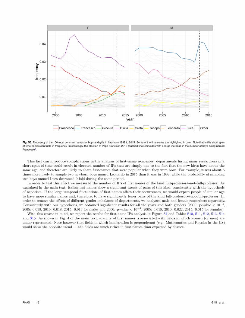
Before presenting the figures and tables for the analysis of first names, we want to highlight an important difference betweenfirst and last names. Last names are passed down from generation to generation, and behave like neutral alleles (with diversitybeing maintained by either immigration or “mutation”—the creation of new last names). First names frequencies, on the otherhand, fluctuate from year to year—certain names become fashionable and increase in frequency, while others decrease (4).These fluctuations can be quite large, and can be caused by well-defined events. For example, in Figure S6 we show thefrequency of the most common names for boys and girls in Italy†, where it is apparent that the election of Pope Franciscoincided with a large increase in the number of boys named Francesco, and a more modest increase in the number of girlsbeing named Francesca.

†Data taken from http://www.istat.it/en/products/interactive-contents/baby-names.‡ Interestingly, the name Giulia grew considerably in popularity in 2003 (and then more modestly in 2004). While it is difficult to pinpoint the cause of this increase, we note that the song “Dedicato a te” by

the Italian band Le Vibrazioni—with its powerful chorus “Sei immensamente Giulia!”—was the top-selling single in March 2003.


F M

0.01

0.02

0.03

0.04

2000 2005 2010 2015 2000 2005 2010 2015year

freq

uenc

y

Francesca Francesco Ginevra Giulia Greta Jacopo Leonardo Luca Other

Fig. S6. Frequency of the 100 most common names for boys and girls in Italy from 1999 to 2015. Some of the time series are highlighted in color. Note that in this short spanof time names can triple in frequency. Interestingly, the election of Pope Francis in 2013 (dashed line) coincides with a large increase in the number of boys being namedFrancesco‡.

This fact can introduce complications in the analysis of first-name isonymies: departments hiring many researchers in ashort span of time could result in elevated number of IPs that are simply due to the fact that the new hires have about thesame age, and therefore are likely to share first-names that were popular when they were born. For example, it was about 6times more likely to sample two newborn boys named Leonardo in 2015 than it was in 1999, while the probability of samplingtwo boys named Luca decreased 9-fold during the same period.

In order to test this effect we measured the number of IPs of first names of the kind full-professor↔not-full-professor. Asexplained in the main text, Italian last names show a significant excess of pairs of this kind, consistently with the hypothesisof nepotism. If the large temporal fluctuations of first names affect their occurrences, we would expect people of similar ageto have more similar names and, therefore, to have significantly fewer pairs of the kind full-professor↔not-full-professor. Inorder to remove the effects of different gender imbalance of departments, we analyzed male and female researchers separately.Consistently with our hypothesis, we obtained significant results for all the years and both genders (2000: p-value < 10−4,2005: 0.018, 2010: 0.018, 2015: 0.019 for males and 2000: p-value < 10−4, 2005: 0.018, 2010: 0.022, 2015: 0.015 for females).

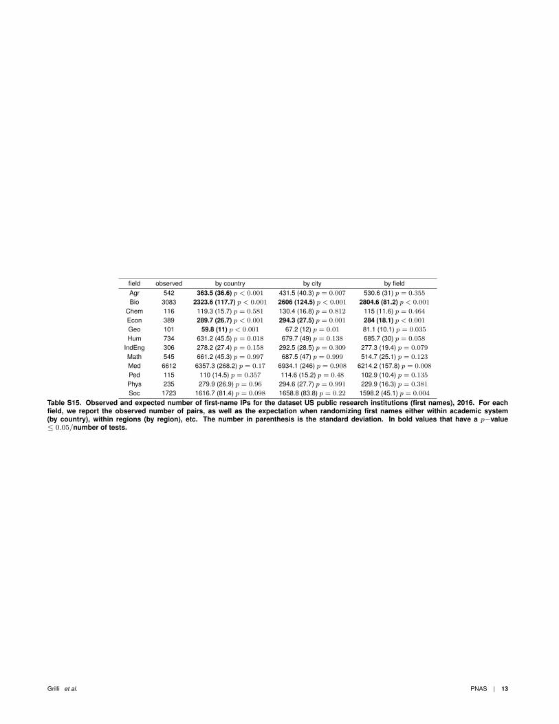
With this caveat in mind, we report the results for first-name IPs analysis in Figure S7 and Tables S10, S11, S12, S13, S14and S15. As shown in Fig. 4 of the main text, scarcity of first names is associated with fields in which women (or men) areunder-represented. Note however that fields in which immigration is preponderant (e.g., Mathematics and Physics in the US)would show the opposite trend — the fields are much richer in first names than expected by chance.


0.0

0.5

1.0

1.5

Agr

Bio

Che

mC

ivEn

g

Econ

Geo

Hum

IndE

ng

Law

Mat

h

Med Ped

Phys

SocObs

erve

d/E

xpec

ted

randomization nation city field

Italy (first names), 2000

0.0

0.5

1.0

1.5

Agr

Bio

Che

mC

ivEn

g

Econ

Geo

Hum

IndE

ng

Law

Mat

h

Med Ped

Phys

SocObs

erve

d/E

xpec

ted



0.0

0.5

1.0

1.5

Agr

Bio

Che

mC

ivEn

g

Econ

Geo

Hum

IndE

ng

Law

Mat

h

Med Ped

Phys

SocObs

erve

d/E

xpec

ted



0.0

0.5

1.0

1.5

Agr

Bio

Che

mC

ivEn

g

Econ

Geo

Hum

IndE

ng

Law

Mat

h

Med Ped

Phys

SocObs

erve

d/E

xpec

ted



0.0

0.5

1.0

Cel

l

Che

m

Eng

Env

Gen

et

Geo

HE

Phys

Hum Info

Mat

h

Neu

ro

PhysObs

erve

d/E

xpec

ted


France CNRS (first names), 2016

0.0

0.5

1.0

1.5

Agr

Bio

Che

m

Econ

Geo

Hum

IndE

ng

Mat

h

Med Ped

Phys

SocObs

erve

d/E

xpec

ted


US public research institutions (first names), 2016

Fig. S7. The same randomizations as in Fig. 1 of the main text, but using first names rather than last names.

field observed by country by city by fieldAgr 1840 1292.4 (70.8) p < 0.001 1471 (80.7) p < 0.001 1552.7 (50.2) p < 0.001Bio 1992 2203.2 (95.9) p = 0.988 2521 (108.9) p = 1 1712.4 (52.1) p < 0.001

Chem 1317 1167.1 (64) p = 0.013 1345.1 (71.4) p = 0.647 1085.3 (40.6) p < 0.001CivEng 2664 2083.5 (107.9) p < 0.001 2312.3 (114.3) p = 0.002 2528.9 (80) p = 0.049Econ 1440 1188.9 (66.2) p < 0.001 1304.4 (69.8) p = 0.032 1288 (48.6) p = 0.002Geo 243 193.8 (19.9) p = 0.01 225.4 (22.5) p = 0.22 209.4 (15.4) p = 0.021Hum 1910 2840.8 (115.2) p = 1 3234.5 (125.2) p = 1 1701 (49.7) p < 0.001

IndEng 4591 2725.1 (125.8) p < 0.001 2942.2 (127.1) p < 0.001 4299.7 (110.3) p = 0.007Law 1600 1360.6 (72) p = 0.001 1603 (83.9) p = 0.5 1494.3 (55.6) p = 0.034Math 934 958.8 (57.1) p = 0.661 1080.2 (61.8) p = 0.993 842.4 (35.6) p = 0.007Med 17983 12061.3 (328.9) p < 0.001 14239.9 (373.4) p < 0.001 15320.8 (261) p < 0.001Ped 1882 2019.7 (97.3) p = 0.923 2286.4 (103.6) p = 1 1667.1 (58.8) p < 0.001Phys 1047 642.6 (43.1) p < 0.001 740.2 (48.7) p < 0.001 859 (36.2) p < 0.001Soc 191 212.8 (22.1) p = 0.844 232.3 (23.1) p = 0.974 194.8 (16.3) p = 0.588

Table S10. Observed and expected number of first-name IPs for the dataset Italy (first names), 2000. For each field, we report the observednumber of pairs, as well as the expectation when randomizing first names either within academic system (by country), within regions (byregion), etc. The number in parenthesis is the standard deviation. In bold values that have a p−value ≤ 0.05/number of tests.

field observed by country by city by fieldAgr 1984 1577.7 (81) p < 0.001 1756 (90.5) p = 0.009 1733.9 (53.9) p < 0.001Bio 2432 2652.6 (107.1) p = 0.986 2986.2 (120.5) p = 1 2073.1 (56.6) p < 0.001

Chem 1249 1141.4 (61) p = 0.044 1309.7 (68.9) p = 0.812 1023.2 (37.8) p < 0.001CivEng 2954 2336.8 (115) p < 0.001 2543.4 (118.5) p < 0.001 2837.7 (91.7) p = 0.105Econ 1811 1531.1 (73) p < 0.001 1713.5 (80.1) p = 0.116 1658.6 (53.4) p = 0.004Geo 215 176.1 (18.2) p = 0.024 203.2 (20.6) p = 0.279 201.6 (15.3) p = 0.197Hum 2139 3079.2 (117) p = 1 3525.4 (129.1) p = 1 1989.1 (53.5) p = 0.004

IndEng 5869 3327.9 (142.7) p < 0.001 3547 (142.5) p < 0.001 5462.4 (136.6) p = 0.003Law 2013 1750.1 (80) p = 0.001 2035.6 (94.4) p = 0.583 1924.7 (58.2) p = 0.07Math 1093 1063.6 (58.3) p = 0.302 1197.6 (64.1) p = 0.954 995.9 (38.1) p = 0.007Med 23755 16770.5 (447.4) p < 0.001 19369.8 (487.8) p < 0.001 20291.7 (385.8) p < 0.001Ped 2143 2285.4 (97.8) p = 0.93 2593.5 (109.5) p = 1 1872.8 (58.9) p < 0.001Phys 1078 659.1 (42) p < 0.001 753.5 (46.9) p < 0.001 896.9 (36.2) p < 0.001Soc 234 269.9 (24.7) p = 0.938 300.6 (26.6) p = 0.998 233.7 (17.5) p = 0.487



field observed by country by city by fieldAgr 1658 1351.3 (70.6) p < 0.001 1509.5 (78) p = 0.034 1395.4 (46.1) p < 0.001Bio 2041 2209.7 (91.2) p = 0.972 2500.8 (105.3) p = 1 1770.4 (49.5) p < 0.001

Chem 1047 896.8 (50.7) p = 0.002 1037.7 (58.4) p = 0.435 813.6 (32.6) p < 0.001CivEng 2320 1979 (104.6) p < 0.001 2123.9 (105.1) p = 0.035 2232.6 (83.2) p = 0.148Econ 1890 1651.2 (72.7) p < 0.001 1822.3 (78.6) p = 0.197 1784.6 (54.3) p = 0.031Geo 162 120 (14) p = 0.003 138.1 (15.9) p = 0.074 143.3 (12.6) p = 0.078Hum 1724 2401.1 (95.1) p = 1 2742 (107.8) p = 1 1635.5 (47.7) p = 0.034

IndEng 6259 3497.6 (147.8) p < 0.001 3730.5 (146.2) p < 0.001 5816.5 (150.1) p = 0.003Law 1864 1659.5 (71.3) p = 0.004 1919.8 (86.2) p = 0.74 1813.7 (53.8) p = 0.177Math 1042 942.2 (50.9) p = 0.029 1058.8 (57.1) p = 0.61 958.6 (36) p = 0.013Med 18336 13694.3 (377.3) p < 0.001 15603.8 (408.8) p < 0.001 15836 (316.6) p < 0.001Ped 2002 2080.2 (91.3) p = 0.807 2365.1 (102.4) p = 1 1735.2 (56.3) p < 0.001Phys 843 501.6 (34.4) p < 0.001 576.2 (38.8) p < 0.001 706.5 (31.5) p < 0.001Soc 253 266.2 (24.2) p = 0.707 301.5 (26.7) p = 0.974 233.7 (17.3) p = 0.137


field observed by country by city by fieldAgr 1467 1227.7 (65) p < 0.001 1384.1 (72.8) p = 0.129 1238.7 (43) p < 0.001Bio 1754 1877.1 (80.6) p = 0.943 2127 (91.8) p = 1 1524.1 (46.4) p < 0.001

Chem 909 760.5 (43.4) p < 0.001 877.2 (51.8) p = 0.254 696.1 (30) p < 0.001CivEng 1794 1580.9 (86.1) p = 0.01 1690 (90.6) p = 0.124 1699.2 (70.6) p = 0.095Econ 1647 1536.5 (69.2) p = 0.064 1698.5 (74) p = 0.748 1589.3 (50.5) p = 0.128Geo 137 97.2 (12.3) p = 0.003 111.7 (13.3) p = 0.04 116.9 (11.6) p = 0.051Hum 1392 1845.4 (78.9) p = 1 2109.1 (89.5) p = 1 1360.4 (43.3) p = 0.228

IndEng 6275 3500.1 (148.9) p < 0.001 3802.5 (149.2) p < 0.001 5695.9 (153.3) p < 0.001Law 1566 1388.5 (62) p = 0.003 1581.7 (72.4) p = 0.58 1525.1 (48.4) p = 0.206Math 935 777.4 (43.9) p < 0.001 876.9 (50.5) p = 0.133 838.7 (33.7) p = 0.002Med 12908 10390.5 (308.9) p < 0.001 11715.8 (331.2) p = 0.001 11283.6 (251.2) p < 0.001Ped 1477 1553.5 (73.5) p = 0.853 1767.7 (82.6) p = 1 1332.2 (46.7) p < 0.001Phys 692 409.8 (29.1) p < 0.001 467.5 (33.7) p < 0.001 585 (27.5) p < 0.001Soc 219 235.1 (21.6) p = 0.772 266.6 (23.7) p = 0.982 203.1 (16) p = 0.165


field observed by country by city by fieldCell 521 444.7 (29.5) p = 0.008 448 (28.4) p = 0.009 447 (23.2) p = 0.001

Chem 1029 844.1 (40.4) p < 0.001 891.9 (38.6) p < 0.001 914.5 (33.8) p < 0.001Eng 624 564.5 (33.4) p = 0.044 607 (27.7) p = 0.265 631.9 (28.7) p = 0.604Env 466 377.7 (25.1) p < 0.001 401.1 (23.7) p = 0.005 425.8 (21.5) p = 0.037

Genet 225 248 (25.8) p = 0.816 257.9 (26.1) p = 0.905 209.5 (17.4) p = 0.196Geo 542 420.7 (27.2) p < 0.001 424.7 (25.9) p < 0.001 516.9 (23.9) p = 0.152

HE Phys 93 95.9 (12.3) p = 0.597 94.6 (11.6) p = 0.563 91.5 (9.5) p = 0.438Hum 1510 1490.3 (50.4) p = 0.344 1485.3 (45.8) p = 0.298 1420.2 (40.6) p = 0.013Info 2875 2327.3 (76.6) p < 0.001 2502.2 (71.7) p < 0.001 2607.5 (61) p < 0.001

Math 955 910 (47.7) p = 0.173 919.2 (45.9) p = 0.218 884.5 (35.3) p = 0.029Neuro 338 317.7 (23.1) p = 0.193 323.1 (22.3) p = 0.261 301.3 (18.1) p = 0.025Phys 479 460.2 (29.5) p = 0.265 472.7 (29.7) p = 0.416 443.8 (23.7) p = 0.074

Table S14. Observed and expected number of first-name IPs for the dataset France CNRS (first names), 2016. For each field, we reportthe observed number of pairs, as well as the expectation when randomizing first names either within academic system (by country), withinregions (by region), etc. The number in parenthesis is the standard deviation. In bold values that have a p−value ≤ 0.05/number of tests.


field observed by country by city by fieldAgr 542 363.5 (36.6) p < 0.001 431.5 (40.3) p = 0.007 530.6 (31) p = 0.355Bio 3083 2323.6 (117.7) p < 0.001 2606 (124.5) p < 0.001 2804.6 (81.2) p < 0.001

Chem 116 119.3 (15.7) p = 0.581 130.4 (16.8) p = 0.812 115 (11.6) p = 0.464Econ 389 289.7 (26.7) p < 0.001 294.3 (27.5) p = 0.001 284 (18.1) p < 0.001Geo 101 59.8 (11) p < 0.001 67.2 (12) p = 0.01 81.1 (10.1) p = 0.035Hum 734 631.2 (45.5) p = 0.018 679.7 (49) p = 0.138 685.7 (30) p = 0.058

IndEng 306 278.2 (27.4) p = 0.158 292.5 (28.5) p = 0.309 277.3 (19.4) p = 0.079Math 545 661.2 (45.3) p = 0.997 687.5 (47) p = 0.999 514.7 (25.1) p = 0.123Med 6612 6357.3 (268.2) p = 0.17 6934.1 (246) p = 0.908 6214.2 (157.8) p = 0.008Ped 115 110 (14.5) p = 0.357 114.6 (15.2) p = 0.48 102.9 (10.4) p = 0.135Phys 235 279.9 (26.9) p = 0.96 294.6 (27.7) p = 0.991 229.9 (16.3) p = 0.381Soc 1723 1616.7 (81.4) p = 0.098 1658.8 (83.8) p = 0.22 1598.2 (45.1) p = 0.004

Table S15. Observed and expected number of first-name IPs for the dataset US public research institutions (first names), 2016. For eachfield, we report the observed number of pairs, as well as the expectation when randomizing first names either within academic system(by country), within regions (by region), etc. The number in parenthesis is the standard deviation. In bold values that have a p−value≤ 0.05/number of tests.


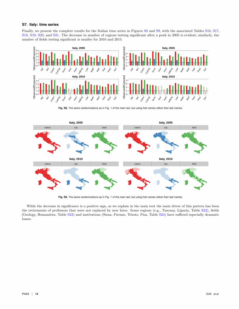
S7. Italy: time series

Finally, we present the complete results for the Italian time series in Figures S8 and S9, with the associated Tables S16, S17,S18, S19, S20, and S21. The decrease in number of regions testing significant after a peak in 2005 is evident; similarly, thenumber of fields testing significant is smaller for 2010 and 2015.

012345

Agr

Bio

Che

m

Civ

Eng

Econ

Geo

Hum

IndE

ng

Law

Mat

h

Med Ped

Phys

SocObs

erve

d/E

xpec

ted


Italy, 2000

01234

Agr

Bio

Che

m

Civ

Eng

Econ

Geo

Hum

IndE

ng

Law

Mat

h

Med Ped

Phys

SocObs

erve

d/E

xpec

ted


Italy, 2005

0

1

2

3

4

Agr

Bio

Che

m

Civ

Eng

Econ

Geo

Hum

IndE

ng

Law

Mat

h

Med Ped

Phys

SocObs

erve

d/E

xpec

ted


Italy, 2010

0

1

2

3

4

Agr

Bio

Che

m

Civ

Eng

Econ

Geo

Hum

IndE

ng

Law

Mat

h

Med Ped

Phys

SocObs

erve

d/E

xpec

ted


Italy, 2015


nation city field

Italy, 2000

nation city field

Italy, 2005

nation city field

Italy, 2010

nation city field

Italy, 2015


While the decrease in significance is a positive sign, as we explain in the main text the main driver of this pattern has beenthe retirements of professors that were not replaced by new hires. Some regions (e.g., Tuscany, Liguria, Table S22), fields(Geology, Humanities, Table S23) and institutions (Siena, Firenze, Trieste, Pisa, Table S24) have suffered especially dramaticlosses.


field observed by country by city by fieldAgr 121 26.6 (5.7) p < 0.001 67.6 (9.6) p < 0.001 28.5 (5.3) p < 0.001Bio 176 45.3 (7.6) p < 0.001 110.9 (12.4) p < 0.001 54.4 (7.6) p < 0.001

Chem 109 24 (5.4) p < 0.001 60.9 (8.9) p < 0.001 26.6 (5.2) p < 0.001CivEng 103 42.9 (7.7) p < 0.001 87.2 (11.5) p = 0.095 45.3 (6.8) p < 0.001Econ 92 24.4 (5.5) p < 0.001 48.1 (7.8) p < 0.001 25.9 (5.2) p < 0.001Geo 19 4 (2.1) p < 0.001 10.7 (3.5) p = 0.023 4.8 (2.2) p < 0.001Hum 103 58.4 (8.7) p < 0.001 125.5 (13.1) p = 0.967 46.6 (6.9) p < 0.001

IndEng 178 56.1 (8.9) p < 0.001 112.2 (13.2) p < 0.001 60.3 (7.9) p < 0.001Law 119 28 (5.8) p < 0.001 68.1 (9.4) p < 0.001 34.3 (6) p < 0.001Math 58 19.7 (4.9) p < 0.001 41.9 (7.3) p = 0.023 21.9 (4.7) p < 0.001Med 832 247.9 (20.3) p < 0.001 620.4 (33.2) p < 0.001 280.7 (17.9) p < 0.001Ped 89 41.5 (7.3) p < 0.001 89.6 (11) p = 0.525 40.2 (6.6) p < 0.001Phys 48 13.2 (3.9) p < 0.001 31 (6.2) p = 0.008 14.8 (3.9) p < 0.001Soc 13 4.4 (2.2) p = 0.002 8.9 (3.2) p = 0.127 4.7 (2.2) p = 0.002


region observed by country by city by fieldAbruzzo 17 5.9 (2.6) p < 0.001 12.2 (3.3) p = 0.103 6.5 (2.7) p = 0.001


Campania 297 62.1 (9.3) p < 0.001 209.1 (15.2) p < 0.001 67.7 (9.6) p < 0.001Emilia-Romagna 192 60.1 (8.9) p < 0.001 135.5 (11.6) p < 0.001 64.2 (9.1) p < 0.001

Friuli-Venezia Giulia 16 8.4 (3.1) p = 0.019 9.7 (3) p = 0.036 8.6 (3.1) p = 0.021Lazio 277 144.4 (16) p < 0.001 189.5 (16.1) p < 0.001 156.9 (16.3) p < 0.001

Liguria 67 20.4 (5.2) p < 0.001 45.3 (6.9) p = 0.003 22.2 (5.3) p < 0.001Lombardia 204 101 (12.3) p < 0.001 165.9 (14.5) p = 0.008 111.2 (12.6) p < 0.001

Marche 13 4.4 (2.2) p = 0.002 10.5 (3.1) p = 0.243 4.7 (2.3) p = 0.003Molise 2 0.3 (0.6) p = 0.046 0.9 (0.9) p = 0.239 0.4 (0.6) p = 0.053

Piemonte 82 41.4 (7.5) p < 0.001 62.8 (8) p = 0.013 44.2 (7.6) p < 0.001Puglia 102 19.5 (4.9) p < 0.001 52.4 (7.1) p < 0.001 20.7 (5) p < 0.001

Sardegna 130 9.8 (3.4) p < 0.001 98.4 (10.2) p = 0.003 10.7 (3.5) p < 0.001Sicilia 425 53.6 (8.5) p < 0.001 304.1 (18.7) p < 0.001 59 (8.8) p < 0.001

Toscana 126 53.2 (8.2) p < 0.001 101.7 (9.8) p = 0.01 56.7 (8.3) p < 0.001Trentino-Alto Adige 3 1.2 (1.1) p = 0.118 1.6 (1.2) p = 0.22 1.3 (1.2) p = 0.134

Umbria 23 8.2 (3.1) p < 0.001 15.2 (3.8) p = 0.035 8.8 (3.2) p < 0.001Veneto 66 38.6 (7.1) p < 0.001 55.2 (7.2) p = 0.081 41 (7.3) p = 0.002

Table S17. Observed and expected number of IPs for the dataset Italy, 2000. For each region, we report the observed number of pairs, as wellas the expectation when randomizing last names either within academic system (by country), within regions (by region), etc. The number inparenthesis is the standard deviation. In bold values that have a p−value ≤ 0.05/number of tests.

field observed by country by city by fieldAgr 146 34.6 (6.6) p < 0.001 88.2 (11.2) p < 0.001 35.6 (6) p < 0.001Bio 209 58.1 (8.6) p < 0.001 143.3 (14.5) p < 0.001 66.9 (8.6) p < 0.001

Chem 109 25 (5.5) p < 0.001 64.4 (9.2) p < 0.001 25.2 (5) p < 0.001CivEng 146 51.2 (8.5) p < 0.001 111.5 (13.4) p = 0.01 58.7 (8) p < 0.001Econ 159 33.6 (6.4) p < 0.001 70.6 (9.5) p < 0.001 35 (6) p < 0.001Geo 17 3.9 (2) p < 0.001 10.6 (3.5) p = 0.056 5.4 (2.3) p < 0.001Hum 134 67.5 (9.3) p < 0.001 152.5 (14.4) p = 0.911 56 (7.6) p < 0.001

IndEng 250 72.9 (10.2) p < 0.001 151.1 (15.8) p < 0.001 81.8 (9.4) p < 0.001Law 179 38.4 (6.8) p < 0.001 96.6 (11.4) p < 0.001 45.4 (6.8) p < 0.001Math 71 23.3 (5.3) p < 0.001 51.4 (8.1) p = 0.015 25.8 (5.1) p < 0.001Med 1093 367.5 (26.8) p < 0.001 851.4 (41.5) p < 0.001 406.5 (22.9) p < 0.001Ped 125 50.1 (8) p < 0.001 114.9 (12.5) p = 0.216 52.7 (7.5) p < 0.001Phys 42 14.4 (4.1) p < 0.001 34.7 (6.6) p = 0.149 14.2 (3.8) p < 0.001Soc 22 5.9 (2.6) p < 0.001 12.5 (3.8) p = 0.016 6.5 (2.6) p < 0.001



region observed by country by city by fieldAbruzzo 26 8.9 (3.2) p < 0.001 17.9 (4) p = 0.036 9.6 (3.3) p < 0.001

Basilicata 6 1 (1) p = 0.002 2 (1.3) p = 0.01 1 (1) p = 0.002Calabria 30 5.4 (2.5) p < 0.001 23.5 (4.5) p = 0.095 5.9 (2.6) p < 0.001

Campania 405 83 (11) p < 0.001 296.9 (19.2) p < 0.001 90.3 (11.2) p < 0.001Emilia-Romagna 213 71.7 (9.8) p < 0.001 152.9 (12.3) p < 0.001 75.8 (9.9) p < 0.001

Friuli-Venezia Giulia 15 9 (3.2) p = 0.05 9.5 (2.9) p = 0.051 9.2 (3.2) p = 0.058Lazio 379 224.9 (22.4) p < 0.001 290.6 (23.2) p = 0.001 245 (21.8) p < 0.001

Liguria 59 19.8 (5.1) p < 0.001 46.1 (6.9) p = 0.043 21.6 (5.2) p < 0.001Lombardia 277 136.8 (14.4) p < 0.001 223.9 (17.2) p = 0.002 150.4 (14.7) p < 0.001

Marche 19 5.8 (2.5) p < 0.001 14.4 (3.6) p = 0.125 6.2 (2.6) p < 0.001Molise 1 0.6 (0.8) p = 0.47 1.3 (1.1) p = 0.743 0.7 (0.9) p = 0.498

Piemonte 110 49 (8.3) p < 0.001 78.8 (9) p = 0.001 52.9 (8.4) p < 0.001Puglia 222 34.7 (6.7) p < 0.001 100 (9.8) p < 0.001 36.9 (6.8) p < 0.001

Sardegna 159 13.4 (4) p < 0.001 124.5 (11.4) p = 0.003 14.5 (4.1) p < 0.001Sicilia 495 65 (9.5) p < 0.001 365.1 (20.2) p < 0.001 70.8 (9.6) p < 0.001

Toscana 166 62.6 (9) p < 0.001 120.5 (10.8) p < 0.001 66.9 (9.1) p < 0.001Trentino-Alto Adige 2 1.9 (1.4) p = 0.557 2 (1.3) p = 0.602 2 (1.5) p = 0.596

Umbria 30 9.2 (3.3) p < 0.001 17.1 (4) p = 0.003 9.8 (3.4) p < 0.001Valle D’Aosta 0 0 (0.2) p = 1 0 (0) − 0 (0.2) p = 1

Veneto 88 43.6 (7.6) p < 0.001 66.7 (8) p = 0.007 46.1 (7.7) p < 0.001Table S19. Observed and expected number of IPs for the dataset Italy, 2005. For each region, we report the observed number of pairs, as wellas the expectation when randomizing last names either within academic system (by country), within regions (by region), etc. The number inparenthesis is the standard deviation. In bold values that have a p−value ≤ 0.05/number of tests.

field observed by country by city by fieldAgr 103 30.9 (6.3) p < 0.001 75.4 (10.2) p = 0.008 29.4 (5.4) p < 0.001Bio 157 50.4 (8.1) p < 0.001 122.3 (13.2) p = 0.008 55.6 (7.7) p < 0.001

Chem 88 20.5 (5) p < 0.001 52.6 (8.2) p < 0.001 20.6 (4.5) p < 0.001CivEng 118 45.2 (8.1) p < 0.001 94.2 (12.3) p = 0.037 51.6 (7.8) p < 0.001Econ 127 37.7 (6.8) p < 0.001 77.9 (10) p < 0.001 38 (6.3) p < 0.001Geo 5 2.7 (1.7) p = 0.148 7 (2.8) p = 0.813 3.1 (1.7) p = 0.191Hum 90 54.8 (8.4) p < 0.001 120.4 (12.6) p = 0.996 47.1 (6.9) p < 0.001

IndEng 227 79.9 (11.1) p < 0.001 157.1 (16.5) p < 0.001 86.3 (10) p < 0.001Law 154 37.9 (6.8) p < 0.001 94.5 (11) p < 0.001 41.7 (6.5) p < 0.001Math 64 21.5 (5.1) p < 0.001 46.7 (7.6) p = 0.019 23.4 (4.9) p < 0.001Med 861 312.7 (24.9) p < 0.001 669.6 (36) p < 0.001 336 (20.9) p < 0.001Ped 109 47.5 (7.9) p < 0.001 100.1 (11.5) p = 0.227 47.7 (7.1) p < 0.001Phys 36 11.5 (3.6) p < 0.001 27.3 (5.8) p = 0.082 12.9 (3.6) p < 0.001Soc 19 6.1 (2.6) p < 0.001 13 (3.8) p = 0.084 7.1 (2.7) p < 0.001



region observed by country by city by fieldAbruzzo 25 9 (3.3) p < 0.001 17.7 (4) p = 0.05 9.5 (3.3) p < 0.001


Campania 317 70 (10) p < 0.001 238.8 (16.9) p < 0.001 74.2 (10) p < 0.001Emilia-Romagna 171 64.4 (9.3) p < 0.001 137.5 (11.6) p = 0.003 66.6 (9.3) p < 0.001

Friuli-Venezia Giulia 12 7 (2.8) p = 0.063 6.4 (2.4) p = 0.025 7.1 (2.8) p = 0.066Lazio 309 200 (21.1) p < 0.001 254.9 (21.2) p = 0.012 212.2 (20.2) p < 0.001

Liguria 41 13.2 (4.1) p < 0.001 33.3 (5.8) p = 0.108 14.1 (4.2) p < 0.001Lombardia 276 140.9 (15) p < 0.001 230.3 (17.8) p = 0.009 150.5 (15) p < 0.001

Marche 21 6.4 (2.7) p < 0.001 15.4 (3.7) p = 0.086 6.6 (2.7) p < 0.001Molise 1 0.7 (0.9) p = 0.509 1.1 (1) p = 0.696 0.7 (0.9) p = 0.522

Piemonte 85 47.2 (8.2) p < 0.001 65.3 (8.1) p = 0.012 49.6 (8.3) p < 0.001Puglia 136 28.1 (6) p < 0.001 73.2 (8.3) p < 0.001 29.1 (6) p < 0.001

Sardegna 141 10.9 (3.6) p < 0.001 108 (10.5) p = 0.002 11.3 (3.6) p < 0.001Sicilia 366 52.2 (8.4) p < 0.001 268.5 (16.7) p < 0.001 55.2 (8.4) p < 0.001

Toscana 119 49 (7.9) p < 0.001 94 (9.6) p = 0.008 51.2 (8) p < 0.001Trentino-Alto Adige 3 2.5 (1.6) p = 0.441 2.4 (1.5) p = 0.43 2.6 (1.7) p = 0.475

Umbria 27 8.9 (3.3) p < 0.001 17.6 (4.1) p = 0.021 9.2 (3.3) p < 0.001Valle D’Aosta 0 0.1 (0.2) p = 1 0 (0) − 0.1 (0.2) p = 1

Veneto 67 41.4 (7.4) p = 0.002 59.1 (7.5) p = 0.162 42.8 (7.4) p = 0.003Table S21. Observed and expected number of IPs for the dataset Italy, 2010. For each region, we report the observed number of pairs, as wellas the expectation when randomizing last names either within academic system (by country), within regions (by region), etc. The number inparenthesis is the standard deviation. In bold values that have a p−value ≤ 0.05/number of tests.

Region 2000 2005 2010 2015 % change (00-05) % change (05-15)Lombardia 6960 8514 8748 8318 22.33 -2.30Lazio 6598 7789 7725 6895 18.05 -11.48Emilia-Romagna 5179 5712 5423 5097 10.29 -10.77Toscana 5019 5439 4850 4087 8.37 -24.86Campania 4593 5559 5524 5074 21.03 -8.72Sicilia 4489 4947 4678 4154 10.20 -16.03Veneto 3386 3694 3622 3446 9.10 -6.71Piemonte 3021 3276 3250 3149 8.44 -3.88Puglia 2388 3317 3095 2826 38.90 -14.80Liguria 1719 1709 1395 1294 -0.58 -24.28Friuli-Venezia Giulia 1624 1724 1535 1398 6.16 -18.91Sardegna 1580 1885 1714 1617 19.30 -14.22Marche 1281 1501 1568 1420 17.17 -5.40Abruzzo 1244 1584 1575 1430 27.33 -9.72Umbria 1157 1251 1231 1174 8.12 -6.16Calabria 863 1177 1372 1330 36.38 13.00Trentino-Alto Adige 417 571 711 775 36.93 35.73Basilicata 322 308 311 305 -4.35 -0.97Molise 164 289 309 263 76.22 -9.00

Table S22. Number of professors by region for the periods considered in the study. The last two columns report the percent change between2000 and 2005 and between 2005 and 2015.

Field 2000 2005 2010 2015 % change (00-05) % change (05-15)Med 9559 11242 10484 9270 17.61 -17.5Hum 5215 5875 5461 4762 12.66 -18.9Bio 4530 5207 4969 4619 14.94 -11.3Hist-Ped-Psi 4164 4954 4859 4248 18.97 -14.2Eng-Ind 4130 4923 5193 5208 19.20 5.8Law 3721 4616 4785 4511 24.05 -2.3Econ 3493 4412 4792 4669 26.31 5.8Eng-Civ 3368 3827 3645 3317 13.63 -13.3Chem 3140 3257 2994 2797 3.73 -14.1Math 2926 3285 3270 2996 12.27 -8.8Agr 2787 3215 3078 2927 15.36 -9.0Phys 2408 2584 2326 2133 7.31 -17.4Soc 1287 1611 1722 1639 25.17 1.7Geo 1276 1280 1114 1006 0.31 -21.4

Table S23. Number of professors by field for the periods considered in the study. The last two columns report the percent change between2000 and 2005 and between 2005 and 2015.


Institution 2000 2005 2010 2015 % change (00-05) % change (05-15)Roma La Sapienza 4246 4656 4230 3574 9.66 -23.2Bologna 2828 3095 2929 2781 9.44 -10.2Napoli Federico II 2673 2983 2683 2359 11.60 -20.9Firenze 2184 2360 2057 1668 8.06 -29.3Padova 2127 2248 2207 2058 5.69 -8.4Milano 1968 2418 2198 1980 22.87 -18.1Torino 1958 2106 2027 1947 7.56 -7.5Pisa 1806 1833 1584 1428 1.50 -22.1Palermo 1795 2018 1797 1554 12.42 -23.0Genova 1719 1709 1395 1294 -0.58 -24.3Bari 1478 1917 1676 1443 29.70 -24.7Catania 1431 1592 1512 1300 11.25 -18.3Cattolica Sacro Cuore 1315 1386 1412 1367 5.40 -1.4Messina 1263 1337 1275 1141 5.86 -14.7Pavia 1119 1132 1029 922 1.16 -18.6Perugia 1117 1199 1172 1116 7.34 -6.9Roma Tor Vergata 1061 1378 1542 1339 29.88 -2.8Politecnico Milano 1014 1264 1360 1316 24.65 4.1Parma 1012 1093 991 915 8.00 -16.3Cagliari 1000 1194 1052 978 19.40 -18.1Trieste 991 945 756 681 -4.64 -27.9Siena 849 1036 943 723 22.03 -30.2Politecnico Torino 785 838 813 804 6.75 -4.1Campania 774 946 1028 959 22.22 1.4Modena e Reggio Emilia 685 846 858 783 23.50 -7.5

Table S24. Number of professors by institutions for the periods considered in the study. The last two columns report the percent changebetween 2000 and 2005 and between 2005 and 2015.


References1. Allesina S (2011) Measuring nepotism through shared last names: the case of Italian academia. PLoS one 6(8):e21160.2. Durante R, Labartino G, Perotti R (2011) Academic dynasties: Decentralization, civic capital and familism in Italian universities. National Bureau of Economic Research, Working paper (No. 17572).3. Zei G, Guglielmino CR, Siri E, Moroni A, Cavalli-Sforza LL (1983) Surnames as neutral alleles: observations in Sardinia. Human Biology pp. 357–365.4. Kessler DA, Maruvka YE, Ouren J, Shnerb NM (2012) You name it–how memory and delay govern first name dynamics. PloS one 7(6):e38790.


last name analysis of mobility, gender imbalance, and ... · and nepotism across academic systems...

Documents