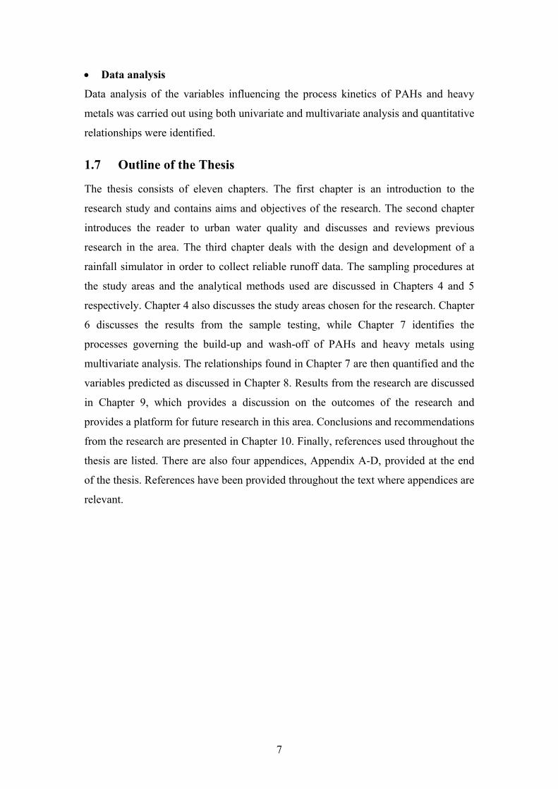
lars herngren phdthesis final - qutfigure 3.7 the rainfall simulator fully mounted on box trailer 53...
TRANSCRIPT
Build-up and wash-off process kinetics of PAHs and
heavy metals on paved surfaces using simulated
rainfall
Lars Herngren MSc Eng. (KTH)
A THESIS SUBMITTED
IN PARTIAL FULFILLMENT OF THE REQUIREMENTS OF
THE DEGREE OF DOCTOR OF PHILOSOPHY
FACULTY OF BUILT ENVIRONMENT AND ENGINEERING
2005

II
Keywords: Urban water quality, Rainfall simulation, Polycyclic Aromatic
Hydrocarbons, Heavy metals, Process kinetics, Build-up, Wash-off.

III
Abstract
The research described in the thesis details the investigation of build-up and wash-off
process kinetics of Polycyclic Aromatic Hydrocarbons (PAHs) and heavy metals in
urban areas. It also discusses the design and development of a rainfall simulator as an
important research tool to ensure homogeneity and reduce the large number of
variables that are usually inherent to urban water quality research. The rainfall
simulator was used to collect runoff samples from three study areas, each with
different land uses. The study areas consisted of sites with typical residential,
industrial and commercial characteristics in the region. Build-up and wash-off
samples were collected at each of the three sites. The collected samples were
analysed for a number of chemical and physico-chemical parameters. In addition to
this, eight heavy metal elements and 16 priority listed PAHs were analysed in five
different particle size fractions of the build-up and wash-off samples. The data
generated from the testing of the samples were evaluated using multivariate analysis,
which reduced the complexity involved in determining the relative importance of a
single parameter in urban water quality. Consequently, variables and processes
influencing loadings and concentrations of PAHs and heavy metals in urban
stormwater runoff from paved surfaces at any given time were identified and
quantified using Principal Component Analysis (PCA). Furthermore, the process
kinetics found were validated using a multivariate modelling approach and Partial
Least Square (PLS) regression, which confirmed the transferability of chemical
processes in urban water quality.
Fine particles were dominant in both the build-up and wash-off samples from the
three sites. This was mirrored in the heavy metal and PAH concentrations at the three
sites, which were significantly higher in particles between 0.45-75μm than in any
other fraction. Thus, the larger surface area and electrostatic charge of fine particles
were favourable in sorbing PAHs and heavy metals. However, factors such as soil
composition, total organic carbon (TOC), the presence of Fe and Mn-oxides and pH
of the stormwater were all found to be important in partitioning of the metals and
PAHs into different fractions. Additionally, PAHs were consistently found in
concentrations above their aqueous solubility, which was attributed to colloidal

IV
organic particles being able to increase the dissolved fraction of PAHs. Hence,
chemical and physico-chemical parameters played a significant role in the
distribution of PAHs and heavy metals in urban stormwater. More importantly, the
research showed the wide range of factors that distribute metals and PAHs in an
urban environment. Furthermore, it indicated the need for monitoring these
parameters in urban areas to ensure that urban stormwater management measures are
effective in improving water quality. The build-up and wash-off process kinetics
identified using PCA at the respective land uses were predicted using PLS and it was
found that the transferability of the governing processes were high even though the
PAHs and metal concentrations and loads were highly influenced by the source
strength at each site. The increased transferability of fundamental concepts in urban
water quality could have significant implications in urban stormwater management.
This is primarily attributed to common urban water quality mitigation strategies
relying on studies based on physical concepts and processes derived from water
quantity studies, which are difficult to transfer between catchments. Hence, a more
holistic approach incorporating chemical processes compared to the current
piecemeal solutions could significantly improve the protection of key environmental
values in a region. Furthermore, urban water quantity mitigation measures are
generally designed to reduce the impacts of high-flow events. This research suggests
that fairly frequent occurring rainfall events, such as 1-year design rainfall events,
could carry significant heavy metal and PAH concentrations in both particulate and
dissolved fractions. Hence, structural measures, designed to decrease quantity and
quality impact on receiving waters during 10 or 20-year Average Recurrence Interval
(ARI) events could be inefficient in removing the majority of PAHs and heavy
metals being washed off during more frequent events.
The understanding of physical and chemical processes in urban stormwater
management could potentially lead to significant improvements in pollutant removal
techniques which in turn could lead to significant socio-economic advantages. This
project can serve as a baseline study for urban water quality investigations in terms
of adopting new methodology and data analysis.

V
List of Publications
Journal Papers
• L. Herngren, A. Goonetilleke, R. Sukpum and D.Y. De Silva (2005) Rainfall
simulation as a tool for urban water quality research. Environmental Engineering
Science, 22 (3), 378-383.
• L. Herngren, A. Goonetilleke and G.A. Ayoko (2005) Understanding heavy
metal and suspended solids relationships in urban stormwater using simulated
rainfall. Journal of Environmental Management, 76 (2), 149-158.
• L. Herngren, A. Goonetilleke and G.A. Ayoko (2004) Multivariate analysis of
heavy metals in road-deposited sediments. Environmetrics. (Under review).
Peer Reviewed International Conference Papers
• L. Herngren, A. Goonetilleke and G.A. Ayoko (2004). Investigation of urban
water quality using artificial rainfall. Watershed 2004, WEF, MWEA, Dearborn,
Michigan, USA, July 2004.
• A.Goonetilleke, E. Thomas, L. Herngren, S. Ginn and D. Gilbert (2004). Urban
water quality: stereotypical solutions may not always be the answer. 2004
International Conference on Water Sensitive Urban Design (WSUD 2004), Cities
as Catchments, IEAust, AWA, Adelaide, Australia, November 2004.
Conference Papers
• L. Herngren, A. Goonetilleke and G.A. Ayoko (2002). Use of rainfall simulation
for urban water quality research. 10th Bi-Annual PIC Postgraduate Conference,
PIC, School of Civil Engineering, QUT, Australia, December 2002.

VI
Table of Contents KEYWORDS II
ABSTRACT III
LIST OF PUBLICATIONS V
ABBREVIATIONS XV
STATEMENT OF ORIGINAL AUTHORSHIP XVII
ACKNOWLEDGEMENTS XVIII
CHAPTER 1 INTRODUCTION 1
1.1 Background 1
1.2 Project Aims and Objectives 2
1.3 Hypotheses 3
1.4 Scope 3
1.5 Justification for the Research 4
1.6 Methodology for the study 5
1.7 Outline of the Thesis 7
CHAPTER 2 URBAN WATER QUALITY 8
2.1 Introduction 8
2.2 Pollutant build-up 9
2.3 Pollutant wash-off 11
2.3.1 First flush phenomenon 12
2.3.2 Influence of rainfall on pollutant wash-off 14
2.4 Common pollutants in an urban environment 18
2.4.1 Pathogens 18
2.4.2 Oxygen demanding wastes 19
2.4.3 Nutrients 20
2.4.4 Suspended solids 21
2.4.5 Heavy metals 24
2.4.6 Polycyclic Aromatic Hydrocarbons 26
2.5 Build-up and wash-off processes of heavy metals 28
2.5.1 Build-up 28

VII
2.5.2 Wash-off 30
2.6 Build-up and wash-off processes of PAHs 34
2.6.1 Build-up 34
2.6.2 Wash-off 35
2.7 Summary 39
CHAPTER 3 DESIGN AND FABRICATION OF A RAINFALL 42
SIMULATOR
3.1 Introduction 42
3.2 Design of a rainfall simulator 43
3.2.1 Re-production of natural rainfall characteristics 44
3.2.2 Structural design 47
3.2.3 Hydraulic System 51
3.2.4 Oscillation Control System 52
3.2.5 Runoff plot and collection 52
3.2.6 Storage and Transport 53
3.3 Performance calibration of the rainfall simulator 53
3.3.1 Nozzle discharge and pattern 54
3.3.2 Rainfall intensities and uniformity of rainfall 56
3.3.3 Calibration of drop size and kinetic energy 62
3.4 Summary 64
CHAPTER 4 STUDY AREAS AND SAMPLING PROCEDURE 66
4.1 Introduction 66
4.2 Study site selection 67
4.3 Project area 67
4.3.1 Residential site 70
4.3.2 Industrial site 71
4.3.3 Commercial site 72
4.4 Vacuum collection system 74
4.4.1 Selection of Vacuum Cleaner 75
4.4.2 Dry collection system efficiency 76
4.4.3 Wet sample collection system 77
4.5 Dry sample collection in the field 81

VIII
4.6 Wet sample collection in the field 82
4.7 Treatment and transport of samples 84
4.8 Summary 84
CHAPTER 5 ANALYTICAL METHODS 86
5.1 Introduction 86
5.2 Sample testing 86
5.2.1 Pre-treatment of samples 86
5.2.2 Particle size distribution 87
5.2.3 Partitioning of samples 89
5.2.4 Chemical and physico-chemical parameters 90
5.3 Summary 97
CHAPTER 6 DISCUSSION OF TEST RESULTS 98
6.1 Introduction 98
6.2 Volume and weight of the collected samples 98
6.3 Particle size distribution 99
6.3.1 Partitioning of build-up and wash-off samples 103
6.4 Chemical parameters 103
6.4.1 pH and EC 103
6.4.2 Organic Carbon 105
6.4.3 Total Suspended Solids 107
6.4.4 Heavy metals 109
6.4.5 Polycyclic Aromatic Hydrocarbons (PAHs) 112
6.5 Summary 117
CHAPTER 7 PATTERN AND PROCESS RECOGNITION 119
USING PCA
7.1 Introduction 119
7.2 Applications of Principal component analysis 119
7.3 Pre-treatment of data 121
7.4 Build-up samples 124
7.4.1 Residential site 124
7.4.2 Industrial site 128

IX
7.4.3 Commercial site 131
7.5 Wash-off samples 134
7.5.1 Residential site 134
7.5.2 Industrial site 144
7.5.3 Commercial site 152
7.6 Summary 159
CHAPTER 8 INVESTIGATING PROCESS KINETICS OF PAHs 163
AND HEAVY METALS USING PCA AND PLS
8.1 Introduction 163
8.2 Application of PCA for prediction of heavy metals and PAHs 164
8.3 Introduction to PLS 172
8.4 Predicting heavy metals and PAHs using PLS1 algorithm 174
8.4.1 Heavy metals in urban stormwater runoff 175
8.4.2 PAHs in urban stormwater runoff 181
8.5 Summary 183
CHAPTER 9 GENERAL DISCUSSION 185
9.1 Rainfall simulation in urban water quality 185
9.2 Chemical processes 186
9.3 Calibration of methodology 187
9.4 Implications of chemical processes found 187
CHAPTER 10 CONCLUSIONS AND RECOMMENDATIONS 189
10.1 Conclusions 189
10.2 Recommendations 192
REFERENCES 194
APPENDIX A RAINFALL SIMULATOR CALIBRATION DATA 217
APPENDIX B TEST RESULTS 235
APPENDIX C CHEMOMETRIC ANALYSIS USING PCA 279
APPENDIX D PREDICTION USING PLS 315

X
List of Figures
Figure 2.1 The effects of urbanisation on hydrological processes 8
Figure 2.2 Hypothetical representation of surface pollutant load over time 12
Figure 2.3 Median drop diameters relationship with rainfall intensity 17
Figure 2.4 Relationship between rainfall intensity and impact energy 17
in South-East Queensland
Figure 3.1 Fan spray pattern nozzle 45
Figure 3.2 Sketch of designed rainfall simulator 48
Figure 3.3 Cross section of the nozzle boom unit 49
Figure 3.4 Catch trays running along the nozzle boom 50
Figure 3.5 Oscillation cycle of the nozzle boom 50
Figure 3.6 Arm and lever system oscillating the nozzle boom 51
Figure 3.7 The rainfall simulator fully mounted on box trailer 53
Figure 3.8 Average discharge values for the twelve Veejet 80100 nozzles 54
(41 kPa pressure)
Figure 3.9 Calibration of spray pattern of the nozzles 55
Figure 3.10 Nozzle spray pattern contours for the chosen nozzles 56
(3, 4 and 12 respectively)
Figure 3.11 Intensity measurements using seven containers 56
Figure 3.12 Container grid pattern used for calculating average rainfall 59
intensity produced by the rainfall simulator
Figure 3.13 Spatial variation of the rainfall intensity using Speed 2, delay 2s 60
Figure 3.14 Pellets obtained by flour pellet method 64
Figure 4.1 Map of Gold Coast region 69
Figure 4.2 Residential research site (Millswyn Crescent) 70
Figure 4.3 Industrial research site (Stevens Street) 72
Figure 4.4 Commercial research site (Centro Nerang) 74
Figure 4.5 Delonghi Aqualand water filter system 76
Figure 4.6 Runoff plot frame used when collecting stormwater samples 79
Figure 4.7 Collection trough with handle to open top for easy sampling 80
using the vacuum cleaner
XI
Figure 4.8 Wet sample collection system showing the connection between 80
25L container and the vacuum cleaner
Figure 4.9 Dry sample collection in the field 81
Figure 4.10 Collection of runoff samples in the field 84
Figure 5.1 Malvern Mastersizer S system used in the project 88
Figure 6.1 Cumulative particle size distribution of the build-up samples 100
collected at the three study sites
Figure 7.1 Scree plot for the determination of number of components to 125
use in exploring residential build-up data
Figure 7.2 Loadings of each variable on PC1 and PC2 obtained from 125
PCA on residential build-up data
Figure 7.3 Loadings of each variable on PC1 and PC2 obtained 129
from PCA on industrial build-up data
Figure 7.4 Loadings of each variable on PC1 and PC2 obtained from 131
PCA on commercial build-up data
Figure 7.5 Loadings of each variable on PC1 and PC2 obtained from 135
PCA on data in the dissolved fraction of wash-off
samples from the residential site
Figure 7.6 Loadings of each variable on PC1 and PC2 obtained from 138
PCA on data in particle size class 0.45-75µm of wash-off
samples from the residential site
Figure 7.7 Loadings of each variable on PC1 and PC2 obtained from 141
PCA on data in particle size class 76-150µm of wash-off
samples from the residential site
Figure 7.8 Loadings of each variable on PC1 and PC2 obtained from 142
PCA on data in particle size class >150µm of wash-off
samples from the residential site
Figure 7.9 Loadings of each variable on PC1 and PC2 obtained from 145
PCA on data in the dissolved fraction of wash-off
samples from the industrial site
Figure 7.10 Loadings of each variable on PC1 and PC2 obtained from 147
PCA on data in particle size class 0.45-75µm of wash-off
samples from the industrial site

XII
Figure 7.11 Loadings of each variable on PC1 and PC2 obtained from 149
PCA on data in particle size class 76-150µm of wash-off
samples from the industrial site
Figure 7.12 Loadings of each variable on PC1 and PC2 obtained from 151
PCA on data in particle size class >150µm of wash-off
samples from the industrial site
Figure 7.13 Loadings of each variable on PC1 and PC2 obtained from 153
PCA on data in the dissolved fraction of wash-off
samples from the commercial site
Figure 7.14 Loadings of each variable on PC1 and PC2 obtained from 155
PCA on data in particle size class 0.45-75µm of wash-off
samples from the commercial site
Figure 7.15 Loadings of each variable on PC1 and PC2 obtained from 157
PCA on data in particle size class 76-150µm of wash-off
samples from the commercial site
Figure 7.16 Loadings of each variable on PC1 and PC2 obtained from 159
PCA on data in particle size class >150µm of wash-off
samples from the commercial site
Figure 8.1 Scores plot of the objects (175 samples) containing heavy 165
metal data subjected to PCA
Figure 8.2 Scores plot of the objects (140 samples) containing PAH data 170
subjected to PCA
Figure 8.3 Cross-validation error (SEV) for Cu showing the number 177
of latent variables to use (2) based on first minimum in plot
Figure 8.4 Plot of observed versus predicted Al concentrations 178
using three latent variables, with an SEP of 0.26
Figure 8.5 Plot of observed versus predicted Al concentrations when 180
Adding additional samples from the commercial site, SEP of 0.56

XIII
List of Tables
Table 2.1 Fraction of pollutants associated with each particle size range, 24
% by weight
Table 2.2 Sources of heavy metals in an urban environment 25
Table 2.3 Priority PAHs as listed by US EPA 27
Table 3.1 Rainfall quality profile obtained in Brisbane, Australia 47
Table 3.2 Calculated average rainfall intensities using seven containers for 57
different speed and delay settings of the control box
Table 3.3 Uniformity coefficients (Cu) for the intensities investigated 61
Table 3.4 Design rainfall events selected 62
Table 4.1 Description of possible residential research sites 70
Table 4.2 Description of possible industrial research sites 72
Table 4.3 Description of possible commercial research sites 73
Table 4.4 Sampling recovery efficiencies 77
Table 4.5 Runoff collection efficiencies 83
Table 5.1 Test methods adopted in the project 91
Table 6.1 Amount of build-up sample collected at each site and respective 98
dry period
Table 6.2 Mass median diameter (d50) in µm of the particles in the 102
simulated runoff events
Table 6.3 pH and EC concentrations of the build-up sample at each site 104
Table 6.4 pH and EC mean concentrations in the EMC-samples for each 105
runoff event
Table 6.5 Total Organic Carbon (TOC) and Inorganic Carbon (IC) 105
recorded in build-up samples from the three study sites
Table 6.6 Mean TOC concentration in wash-off samples 107
Table 6.7 TSS concentrations in the build-up samples 108
Table 6.8 TSS mean concentrations in the wash-off samples 108
Table 6.9 Heavy metal concentrations in each particle size class 110
at the three sites
Table 6.10 Metal concentration ranges observed in particulate and 112
dissolved fractions of wash-off samples from each site

XIV
Table 6.11 PAH concentration (mg/kg) in the build-up samples from each 114
site
Table 6.12 Detection frequencies (%), mean concentrations (mg/kg) and 116
standard deviation of 16 PAHs in wash-off samples from the
residential, industrial and commercial site
Table 7.1 Parameter abbreviation as used in PCA 123
Table 8.1 Variables and objects associated with negative and positive 168
loadings and scores on PC3 (excluding build-up and dissolved)
Table 8.2 Variables to be predicted (Y) and predictor variables (X) 176
Table 8.3 Calibration and validation matrices for prediction of metals 176
Table 8.4 Number of latent variables used for each predicted variable 178
Table 8.5 r2 and SEP values generated from the predictions (metals) 179
Table 8.6 Variables to be predicted (Y) and predictor variables (X) 181
Table 8.7 Number of latent variables used for each predicted variable 182
Table 8.8 r2 and SEP values generated from the predictions (PAHs) 183

XV
Abbreviations
ACE Acenaphthene
ACY Acenaphthylene
Al Aluminium
ANT Anthracene
ARI Average Recurrence Interval
BaA Benzo[a]Anthracene
BaP Benzo[a]Pyrene
BbF Benzo[b]Flouranthene
BgP Benzo[g,h,i]Perylene
BkF Benzo[k]Flouranthene
BOD Biological Oxygen Demand
Cd Cadmium
CHR Chrysene
COD Chemical Oxygen Demand
Com Commercial site
Cr Chromium
Cu Copper
DbA Dibenzo[a,h]Anthracene
DC Dissolved Carbon
DCM DiChloroMethane
DCM:ACE DiChloroMethane: Acetone
DOC Dissolved Organic Carbon
EC Electrical Conductivity
EMC Event Mean Concentration
Fe Iron
FLA Flouranthene
FLU Flourene
GC-MS Gas Chromatograph – Mass Spectrometer
HNO3 Nitric Acid
IC Inorganic Carbon

XVI
ICP-MS Inductively Coupled Plasma – Mass Spectrometer
Ind Industrial site
IND Indeno[1,2,3-cd]Pyrene
Mn Manganese
N2 Nitrogen
NAP Naphthalene
Ni Nickel
PAH Polycyclic Aromatic Hydrocarbon
Pb Lead
PC Particulate Carbon
PCA Principal Component Analysis
PHE Phenanthrene
POC Particulate Organic Carbon
ppm parts per million
PRESS Predicted Residual Error Sum of Squares
PVP Particle Volume Percentage
PYR Pyrene
Res Residential site
SEP Standard Error of Prediction
SEV Standard Error of Validation
TDS Total Dissolved Solids
TOC Total Organic Carbon
TSS Total Suspended Solids
US EPA United States Environmental Protection Agency
Zn Zinc

XVII
Statement of Original Authorship
The work contained in this thesis has not been previously submitted for a degree or
diploma for any other higher education institution to the best of my knowledge and
belief. The thesis contains no material previously published or written by another
person except where due reference is made.
Signed:
Lars Herngren
Date: / /

XVIII
Acknowledgements
I wish to express my sincere appreciation to my Principal Supervisor A/Prof.
Ashantha Goonetilleke for his guidance, support and professional advice during the
study. Special thanks are also given to my Associate Supervisor Dr. Godwin Ade
Ayoko for his guidance and professional support throughout the research. Special
thanks are extended to Åke and Greta Lissheds Stiftelse, J. Gust. Richerts Stiftelse
and the Faculty of Built Environment and Engineering at QUT for financial support
during my candidature.
Appreciation is extended to all staff in the School of Civil Engineering and special
thanks to Mr. Brian Pelin and Mr. Jim Grandy for manufacturing the rainfall
simulator. Appreciation is also extended to Mr. Arthur Powell for electronic controls
of the rainfall simulator. I would like to thank Dr. Serge Kokot for advice on
analytical procedures. Appreciation is also extended to the professional staff of the
School of Physical and Chemical Sciences for technical support in GC-MS and
extraction and digestion procedures of PAHs and heavy metals.
I would also like to thank Adjunct Prof. Evan Thomas of Gold Coast City Council
and Mr. Don Pegler and Mr. Mark Silburn of the Department of Natural Resources,
Toowoomba for invaluable feedback on the design of a rainfall simulator. Also
thanks to Dr. Rob Loch at Landloch for showing rainfall simulator designs.
I wish to express my gratitude and appreciation to my father (Stig-Olof) and mother
(Ulla-Britt) for their unlimited support and love. I would also like to thank my sister
with family and all of my friends for support. Lastly, in acknowledgement of the
loving support and constant encouragement extended to me, I would like to thank my
loving partner Brianna Casey.
1
Chapter 1 Introduction
1.1 Background
Urbanisation is a common phenomenon witnessed in most parts of the world,
transforming natural and rural environments and often dramatically altering local
hydrological conditions. This is primarily attributed to the increase of impervious
surfaces and the rate of transport of pollutants into waterways, which could lead to
significant degradation of the quality of receiving waters. Therefore, it is imperative
that innovative strategies are adopted to ensure the protection of key environmental
values. Consequently, appropriate management of urban stormwater runoff has
significant positive socio-economic and environmental implications.
Multiple variables and processes are involved in the generation and transport of
pollutants in urban environments. The variables involved are highly dependent on a
number of characteristics, which are often subject to uncertainty. The weighting or
relative importance of the characteristics involved is often hard to measure and is
highly variable within the urban environment. This has led to limitations in the
transferability of previous research. Knowledge of these characteristics and variables
is the base for successful mitigation of urban stormwater quality impacts on receiving
waters. This is particularly important for micro-pollutants such as Polycyclic
Aromatic Hydrocarbons (PAHs) and heavy metals due to the toxic nature of these
compounds. Furthermore, PAH and heavy metal pollution has been identified as
leading causes of the degradation of receiving waters (Sansalone and Buchberger
1997; Estebe et al. 1997).
The availability of more reliable methodology in urban stormwater will prove
invaluable in the development of management strategies to protect or improve the
existing quality of receiving waters. Retrofitting of existing urban developments for
stormwater quality improvement and the analysis of ‘what if’ scenarios in the
evaluation of land development alternatives and catchment management strategies
will be greatly enhanced with the availability of more reliable modelling capabilities.
It is in this regard that research methodologies commonly used in other disciplines,
such as agriculture, should be adapted and implemented. The use of small test plots to

2
ensure homogeneity and tools such as artificial rainfall simulators could help to
reduce the large number of variables which are usually inherent to urban water quality
research. The use of artificial rainfall has been a common approach in agricultural
research to overcome the lack of data in infiltration, runoff and erosion studies.
However, the application of artificial rainfall in urban water quality research is rarely
mentioned, even though it can significantly improve the transferability of water
quality studies. Hence, it is imperative to find an equally efficient tool in urban water
quality studies. It is a primary hypothesis of this research that rainfall simulation is
capable of improving the quantification of the factors influencing the process kinetics
of PAHs and heavy metals in urban stormwater.
1.2 Project Aims and Objectives
The major aims of this study were to evaluate the influence of physical and chemical
parameters in the distribution of PAHs and heavy metals in build-up and wash-off
from paved surfaces. In addition, the project aimed at assessing the use of rainfall
simulation in developing a reliable urban runoff water quality database. In summary,
the aims of the study were:
1. to develop a rainfall simulator for applying artificial rainfall on a paved surface;
and
2. to develop an in-depth understanding of the build-up and wash-off process
kinetics of PAHs and heavy metals using a number of simulated rainfall events
and multivariate chemometrics techniques.
The primary objectives of the study were:
1. to confirm the validity of using rainfall simulation in urban water quality research;
2. to evaluate the build-up and wash-off process kinetics of PAHs and heavy metals
on urban paved surfaces for different land uses; and
3. to determine the influence of particle size of suspended solids on urban water
quality in relation to PAHs and heavy metals.
1.3 Hypotheses
• The use of rainfall simulation significantly improves the collection of reliable
urban stormwater samples for the analysis of chemical processes inherent to urban
water quality.

3
• Parameters such as suspended solids and dissolved organic carbon significantly
influence the build-up and wash-off process kinetics of PAHs and heavy metals.
• Fine particles carry a significant load of PAHs and heavy metals in urban runoff.
• The understanding of chemical processes facilitates the transferability of urban
water quality research.
1.4 Scope
The primary focus of this research was the surface runoff generated by rainfall events
where a significant fraction of built-up pollutants is transported to receiving waters.
The research investigated the processes involved in distributing PAHs and heavy
metals in the build-up and wash-off from three different urban areas. The research
undertaken was confined to the Gold Coast City Council area, but the processes and
relationships found are applicable anywhere. The research was confined to paved
surfaces in industrial, residential and commercial areas. Pavement characteristics were
not considered as influencing parameters in the research but were used merely as a
classification of the pavement condition at the respective research sites. This was
based on the hypothesis that chemical processes are independent of parameters such
as pavement roughness, permeability and slope. Consequently, the build-up and wash-
off process kinetics of PAHs and heavy metals were considered unaffected by
pavement parameters. However, it is important to note that the pollutant load reaching
receiving waters could vary depending on the pavement characteristics. Hence, the
concentrations and loads of PAHs and heavy metals found in wash-off from less
permeable and smooth surfaces could be significantly higher than concentrations in
wash-off from permeable rough surfaces.
A rainfall simulator, which was accurately calibrated to reproduce natural rainfall
characteristics in the study area, was used to generate the runoff from the paved
surfaces. Artificial rainfall was applied to a small homogenous plot area, which
reduced the number of physical factors involved in the wash-off process.
The project specifically focused on the wash-off of PAHs and heavy metals from
paved surfaces using artificial rainfall. Natural rainfall and runoff events were not
investigated due to insufficient time to collect a similarly reliable database.
4
Additionally, the performance of urban stormwater management measures was not
investigated.
Three different land uses were selected as representative sites and twelve different
rainfall events were simulated at each site. Only one site per land use was chosen.
This was based on the hypothesis that chemical processes are independent of the
pollutant load in an area. Consequently, the density of industries and the traffic
volume was not considered to be determining factors in build-up and wash-off process
kinetics other than influencing the total load available on a paved surface. Hence, the
chosen sites represented typical industrial, residential and commercial characteristics
in the study region and the process kinetics found was considered applicable to any
area. A build-up sample was also collected at the time of the field study and analysed
accordingly. There is limited knowledge available on processes governing the
distribution of PAHs and heavy metals into different particle size classes. As a result,
the runoff generated from each event was separated into a dissolved and a particulate
phase. The particulate phase was further partitioned into four different particle size
classes and analysed individually for chemical characteristics to fill the gaps in the
understanding of water quality processes.
1.5 Justification for the Research
Urbanisation can dramatically alter environmental conditions in a catchment,
particularly the generation and transport of pollutants such as PAHs and heavy metals
on impervious surfaces, thereby adversely changing the quality of water. Though
limited research has been undertaken on the wash-off of pollutants from paved
surfaces, these investigations have been significantly constrained. This has primarily
been attributed to the limited understanding of interactions between various influential
parameters and the influence of chemical processes on the build-up and wash-off
process kinetics of PAHs and heavy metals. Consequently, the management of water
quality impacts in urban areas has proven to be a difficult task.
Unfortunately, in the past, urban water quality models have been strongly based on
water quantity research. Hence, the extension of concepts and processes from water
quantity studies has been used to predict the pollutant generation, dispersion and
transmission in an urban environment. This has led to the reliance on physical factors

5
and limited recognition of chemical processes underlying the build-up and wash-off of
PAHs and heavy metals. Chemical processes exert a strong influence on the quality
characteristics of urban stormwater. It is this oversight which can be attributed to the
often contradictory results reported in research studies and the strongly location
specific nature of outcomes. Additionally, in past research, the general focus has been
on the build-up and wash-off of pollutants in relatively large heterogeneous areas.
Very little work has been undertaken using small, homogenous catchment areas in
order to fully understand the process kinetics of PAH and heavy metals in urban
stormwater.
Data analysis using multivariate chemometrics methods can significantly enhance the
outcomes of water quality studies. This is attributed to the large number of variables
involved in the build-up and wash-off process kinetics. Consequently, univariate
statistical analysis such as linear regression is useful when two variables are compared
against each other. However, the processes inherent in the generation and transport of
pollutants are many and often complementary. Hence, tools that take more than one
variable into account when analysing the build-up and wash-off process kinetics of
PAHs and heavy metals are preferable and can significantly enhance the
understanding of influential parameters in urban stormwater. This study was
formulated to create an improved methodology for urban water quality studies and to
increase the knowledge of processes governing the distribution of PAHs and heavy
metals in urban build-up and wash-off.
1.6 Methodology for the study
The objectives of the research project were achieved through the following steps:
• Design and development of a rainfall simulator
Rainfall simulation is not new to water research. However, it has essentially been
confined to the agricultural arena. Rainfall simulation provides maximum control over
when and where data is to be collected, plot conditions at test time and rates and
amounts of rainfall to be applied to the test plot. The major challenges transferring
rainfall simulation techniques used in agricultural research to urban water quality
research are:
1. the collection of runoff from paved surfaces; and

6
2. the portability of the rainfall simulator, not only from plot to plot but from site to
site.
The design and development of the rainfall simulator was the basis for the site
selection and broad-scale field investigations to be undertaken.
• Study site selection and selection of rainfall events
The study sites selected were representative of characteristics for typical urban areas
in the region. One site per land use was chosen as below:
1. Light Industrial
2. Commercial
3. Residential
Twelve different rainfall events were chosen to be simulated at each of the sites.
These were based on actual rainfall intensities and durations for South-East
Queensland and consisted of 1, 2, 5 and 10-year ARI design rainfall events. The
rainfall simulator was precisely calibrated for each event simulated.
• Data collection/compilation
Physical, physico-chemical and chemical parameters were measured for the samples
collected from the simulated rainfall events at each site. The parameters were chosen
based on factors influencing the generation and transport of PAHs and heavy metals
in the urban environment.
• Sample testing
Build-up and wash-off samples were tested for water quality parameters according to
methods set out by relevant authorities in order to ensure accuracy in the results.
Quality control was an important measure in the analysis of water quality samples.
Full procedural blanks and spiked samples were used to verify the absence of matrix
interferences as specified by relevant water quality sampling and testing methods.
7
• Data analysis
Data analysis of the variables influencing the process kinetics of PAHs and heavy
metals was carried out using both univariate and multivariate analysis and quantitative
relationships were identified.
1.7 Outline of the Thesis
The thesis consists of eleven chapters. The first chapter is an introduction to the
research study and contains aims and objectives of the research. The second chapter
introduces the reader to urban water quality and discusses and reviews previous
research in the area. The third chapter deals with the design and development of a
rainfall simulator in order to collect reliable runoff data. The sampling procedures at
the study areas and the analytical methods used are discussed in Chapters 4 and 5
respectively. Chapter 4 also discusses the study areas chosen for the research. Chapter
6 discusses the results from the sample testing, while Chapter 7 identifies the
processes governing the build-up and wash-off of PAHs and heavy metals using
multivariate analysis. The relationships found in Chapter 7 are then quantified and the
variables predicted as discussed in Chapter 8. Results from the research are discussed
in Chapter 9, which provides a discussion on the outcomes of the research and
provides a platform for future research in this area. Conclusions and recommendations
from the research are presented in Chapter 10. Finally, references used throughout the
thesis are listed. There are also four appendices, Appendix A-D, provided at the end
of the thesis. References have been provided throughout the text where appendices are
relevant.

8
Chapter 2 Urban Water Quality
2.1 Introduction
Urbanisation in a catchment results in an increased percentage of impervious surfaces
such as roads and roofs. Consequently, during rainfall, this leads to an increase in both
water quantity and water quality impacts as illustrated in Figure 2.1 adapted from Hall
(1984).
FIGURE 2.1 The effects of urbanisation on hydrological processes (adapted
from Hall 1984)
The increased flood frequency of urban areas due to the increased runoff volume and
decreased time to peak has been confirmed by numerous researchers (McPherson
1974; Corbett et al. 1997). However, hydrologic and water quality models used to
predict pollutant generation and transport in urban environments require input
parameters that are not known with certainty (Sohrabi et al. 2002). The relationships
developed are largely physically based and inadequate for describing the chemical
processes that take place. This relates not only to the outcomes of previous studies but
also to the conducting of research. Hence, a multi disciplinary approach to a typical
Urbanisation
Population density increases
Building density increases
Waterborne waste increases
Water demand rises
Impervious area increases
Water resource problems
Drainage system modified
Urban climate changes
Stormwater quality deteriorates
Groundwater recharge reduces
Runoff volume increases
Flow velocity increases
Receiving water quality deteriorates
Baseflow reduces Peak runoff rate increases
Lag time and time base reduce
Pollution control problems
Flood control problems

9
engineering problem could provide complementary information and facilitate
transferability of the processes found.
Chemical processes exert a strong influence on urban stormwater quality
characteristics. However, the common oversight of these processes has led to
contradictory results being reported in research studies and a strong location specific
nature of outcomes. This has led to inadequate knowledge of the processes
influencing the wash-off of micro-pollutants such as PAHs and heavy metals in an
urban catchment. This is of particular concern due to the toxic nature of these
pollutants, which have also been identified as the leading cause of the degradation of
receiving waters (Estebe et al. 1997; Sansalone and Buchberger 1997). Furthermore,
most research studies generally report on the total amount of PAHs or heavy metals
present without regard to their physical or chemical state, such as whether they are
tied up into complex inorganic or organic compounds. As water quality models are
increasingly used to evaluate management issues in catchments, there is an increasing
need to assess the processes taking place during urban stormwater runoff.
Consequently, the management of water quality impacts in urban areas has proven to
be a difficult task and the effectiveness of commonly adopted management and
structural measures is open to question.
While not consisting of a substantial portion in most urban catchments, except in
highly commercial areas, the effects of paved surfaces are important for
understanding the quality of stormwater. Examples are the traffic on roads, which
results in deposition of vehicular related particulates on road surfaces for subsequent
removal by wash-off processes; and the role of paved surfaces in acting as flow paths
for stormwater runoff. Additionally, many small rainfall events result in runoff
occurring only from these paved surfaces (Corbett et al. 1997; McPherson 1974).
This chapter focuses on the processes governing the build-up and wash-off of
pollutants on paved surfaces. Special attention is given to the processes involving
PAHs and heavy metals, which are discussed in Section 2.5 and 2.6 respectively. This
chapter also discusses the common sources of pollutants, and identifies important
physical and chemical variables which influence build-up and wash-off processes.

10
2.2 Pollutant build-up
Build-up is defined as the accumulation of pollutants on catchment surfaces during
antecedent dry periods. Pollutants are generated by a variety of anthropogenic
activities and natural phenomena in an urban environment. The pollutants introduced
are later washed out by rainfall and the runoff transports the pollutants to receiving
waters. As noted by Sartor and Boyd (1972), build-up of pollutants is a dynamic
process in urban areas. Hence, if there is sufficient antecedent time for build-up to
occur, the pollutant availability on a paved surface is likely to remain largely the same
(Duncan 1995). The natural sources vary significantly within catchments and include
water-transported material from surrounding soils, dry and wet atmospheric
deposition and biological inputs from vegetation (Sutherland and Tolosa 2000;
Muschack 1990; Rogge et al. 1993). Significant quantities of particulate matter can be
attributed to anthropogenic sources such as industrial processes, vehicle emissions
and, tyre and road surface wear (Sartor and Boyd 1972; Rogge et al. 1993). In urban
areas, particulates derived from automobiles and local soils have been identified as the
dominant sources of pollutant accumulation on a paved surface (Tai 1991; Shaheen
1975). However, the relative importance of these sources depends significantly on site
characteristics such as the fraction of impervious surfaces and traffic conditions.
Dirt or soil is tracked onto streets, for example, by vehicles leaving unpaved
construction sites or simply by the wind blowing garden soil particles onto the paved
surfaces. Because streets are usually built for vehicles, particulate automobile exhaust,
lubricating oil residues, tyre wear particles, weathered street surface particles, and
brake lining wear are direct contributors to the road dust. Indirectly, via atmospheric
transport and fallout, practically any anthropogenic or natural source can add to the
street dust accumulation on a road surface.
The contribution of soil to the accumulation of particulates can be significant. Hopke
et al. (1980) found that 76% of the total street dust mass originated from soil
materials. Similarly, Tai (1991) found that most of the street surface particles
originated from the erosion of local soils. However, the contribution of local soils to
the build-up component in urban stormwater is highly variable and depends on a
number of factors such as the amount of topsoil present and the fraction of impervious

11
surfaces. Similarly, the contribution from anthropogenic sources to the build-up
component is also highly variable within urban areas due to the amount of physical
and geographical factors removing and re-depositing material. The build-up
component of urban stormwater on paved surfaces from both natural and
anthropogenic sources is dependent on primary factors such as:
• Climate including rainfall and wind
• Land use
• Population density
• Percentage impervious area
• Traffic characteristics
• Antecedent dry period
• Street cleaning practices
• Soil type
(Sartor and Boyd 1972; Ball et al. 1998; Brezonik and Stadelmann 2002)
Though the build-up component is dependent on a number of factors, the degree of
influence that these factors exert is highly variable, which significantly constrains the
relative importance of a single parameter in the build-up process. Additionally, a large
homogenous data set is needed to create reliable and predictive relationships between
parameters. Consequently, build-up studies involving a large number of physical and
geographical parameters can be very site-specific and the outcomes can be hard to
transfer to other areas. Hence, the reduction of the number of statistically significant
physical factors could significantly facilitate transferability of research.
2.3 Pollutant wash-off
Pollutants are incorporated into stormwater runoff via wash-off processes. Pollutant
wash-off is influenced by the amount of pollutants available, which in turn is
determined by the build-up process. Since the build-up process is in dynamic
equilibrium (as noted in Section 2.2), the pollutant availability on the catchment
surface for wash-off is likely to remain largely the same. Hence, pollutant build-up
and wash-off show a strong interaction.

12
Vaze and Chiew (2002) proposed two possible alternative pollutant wash-off models
as illustrated in Figure 2.2. The outcomes from their field study, conducted on an
impervious surface in Melbourne Australia, indicated a relatively quick pollutant
accumulation rate after a rain event. However, the rate slowed down after several days
and stayed fairly constant until a cleansing event occurred, as illustrated in Figure
2.2(b). The alternative view to the pollutant accumulation process is illustrated in
Figure 2.2(a), where the surface pollutant load builds up from zero over the
antecedent dry days. Most of the available load is then washed off during a storm
event. Hence, the build-up of pollutants is based on measurements of pollutant wash-
off only. For example, Ball (2000) found that events with an average intensity greater
than 7mm/hr could be considered as cleansing events. Unfortunately, this alternative
view has been adopted in water quality models even though studies have shown that a
storm event may typically only remove a small proportion of the overall surface
pollutant load (Chiew et al. 1997; Malmquist 1978).
FIGURE 2.2 Hypothetical representations of surface pollutant load over time
(adapted from Vaze and Chiew 2002)
The wash-off load is dependent on parameters such as rainfall duration, texture depth
of the runoff surface and the particle size distribution of the accumulated material
(Andral et al. 1999). Thus, there are a number of physical and chemical factors
preventing the pollutant load on a paved surface from returning to zero.
Similarly, Duncan (1995) proposed that the wash-off pollutant load varies throughout
the rain event as a function of rainfall intensity or runoff velocity and would not in
general demonstrate an exponential or linear relationship with runoff volume, rainfall
intensity or pollutants remaining. Hence, exponential or linear wash-off functions
cannot simulate an increase in pollutant concentration at any time during the storm.
13
This would be a situation where a higher order storm can lead to enhanced pollutant
detachment rather than a proportionate increase.
2.3.1 First flush phenomenon
Numerous researchers have reported the first flush as an important phenomenon, as
this is the runoff component that is the most contaminated during a storm event (Lee
et al. 2002). It is defined as the initial period of stormwater runoff during which the
concentration of pollutants is substantially higher than during other stages. However,
Lee and Bang (2000) found that the pollutant concentration peak followed the flow
peak in watersheds that only had an impervious area less than 50% of the total area.
They also found that the concentration peak may vary for different pollutants during a
storm event. As Duncan (1995) has postulated, there is a significant possibility that
different processes dominate under different conditions or at different scales.
The significance of the first flush stems from the fact that management practices such
as detention and retention basins are often designed for the initial component of urban
stormwater. Hence, economic implications in relation to management and treatment
of urban stormwater are incorporated with the first flush. Although the occurrence of
first flush has been confirmed in most instances, the observations noted are not
consistent. Numerous researchers have reported widely varying behaviour of different
pollutants. Additionally, numerous other researchers have claimed that the
significance of first flush is overrated and not all storms exhibit the first flush
phenomenon (Hall and Ellis 1985; Sonzogni et al. 1980).
Hoffman et al. (1984) found that suspended solids exhibited proportionate peaks
during a runoff event with three flow peaks. This was mirrored by the total particulate
hydrocarbon concentration. However, individual hydrocarbons showed different
peaks, with different species showing peak concentrations throughout the runoff
event. A number of factors have been attributed to this behaviour, such as solubility,
volatility, susceptibility to degradation and differences in particle size distribution of
the solids. Similarly, particulate bound metals have been found to exhibit a first flush
whilst the major fraction of the dissolved fraction is transported during the middle of
the storm event (Hall and Anderson 1986; Sansalone and Buchberger 1997). Harrison

14
and Wilson (1985) noted that the physico-chemical associations in which pollutants
are present exert a strong influence on the first flush effect of various pollutants.
As suggested by Ellis (1991), the concentration peaks of pollutants occur in the first
flush, however the pollutant load of the first flush contributes on average only 30-35%
of the total pollutant load. Instead, high correlations between maximum pollutant load
and peak flow have been observed, even though the pollutant concentration declines
with time (Ball 2000; Herrmann 1981; Morrison et al. 1984). Similarly, Hoffman et
al. (1985) found pollutant load peaks of hydrocarbons, heavy metals and suspended
solids coincide with the runoff peak.
The contribution of the first flush is also dependant on catchment characteristics, in
addition to rainfall intensity and runoff volume. The strength of the first flush has also
been found to be more pronounced in small rather than large catchments (Lee and
Bang 2000; Lee et al. 2002). However, the analysed catchments had a significantly
different percentage of impervious surfaces (Small: 80% impervious; Large: 50%
impervious) questioning the relationship between catchment size and the significance
of the first flush. This is supported by Bertrand-Krajewski et al. (1998) who suggested
that the influence of catchment size on first flush strength was minor. Additionally,
pollutants in a larger catchment would be more susceptible to processes such as
dispersion and diffusion due to the increased number of pollutant obstructions, which
makes the contaminant plume spread out. Hence, as contamination spreads out as it
moves, it does not arrive all at once at a given location downstream.
As the above discussion highlights, the reported results from various studies are
confusing and constrain the development of rational concepts to describe the first
flush, mostly due to the difference in quantifying the first flush in the studies. This is
mirrored in the uncertainty of key assumptions in urban water quality models.
2.3.2 Influence of rainfall on pollutant wash-off
The development of water quality models has been closely linked to water quantity.
Understanding the relationship between water quality and water quantity is important
for two main reasons.

15
Firstly, in most water quality models, pollutant concentration and pollutant load
cannot be estimated without the estimation of flow. The flow factor in urban runoff
pollution has been identified as the driving force in the mobilisation, transport and
deposition of pollutants due to the superimposed effect of an urbanised catchment on
flow characteristics (Ellis 1985). Secondly, procedures to mitigate water quantity and
water quality problems are often complementary. Conversely, the procedures for the
estimation of water quantity and water quality in an urban area differ largely from a
rural area due to the large proportion of impervious areas in an urban environment
(Zoppou 2001).
Influence of rainfall characteristics on the wash-off of pollutants is important due to
two primary processes. Firstly, as rainfall hits the ground, it initially wets the surface
and begins to dissolve water soluble pollutants. The impacting raindrops and
horizontal sheet flow provide the necessary turbulence for dissolving the soluble
fraction. Secondly, the pollutants detach as a result of rainfall impact and are
transported by surface runoff. By undertaking impact energy tests on rainfall on paved
surfaces, Vaze and Chiew (1997) showed that both the turbulence created by falling
raindrops and the shear stress imparted by runoff were important in loosening the
surface particles and suspending them in water. Depending on the intensity and
duration of the storm, part of the available surface pollutant load becomes
disintegrated and/or dissolved (Vaze et al. 1997).
It has also been found that rainfall itself is a significant source of some pollutants,
especially nitrogen species (Ebbert and Wagner 1987; Drapper et al. 2000). Similarly,
Brezonik and Stadelmann (2002) found that rainfall in Eastern Minnesota contributed
up to half the concentration of nitrate and ammonium found in roadway runoff. Low
levels of PAHs have also been detected in rainfall, especially in precipitation
occurring in industrial areas (Polkowska et al. 2000). However, as Herrmann (1981)
has noted, the concentrations of PAHs in rainfall are low compared to the
concentrations of PAHs in urban stormwater runoff.
Higher loads of pollutants reaching receiving waterways have been associated with
higher amounts of rainfall (Bruwer 1982). For example, Lee and Bang (2000) found
that concentration levels of suspended solids and chemical oxygen demand rose

16
significantly with increasing runoff, independent of land use. On the contrary, in an
extensive study of stormwater runoff data from 68 catchments in areas surrounding
Minnesota USA, it was found that rainfall duration was negatively correlated with
pollutant concentrations and loads (Brezonik and Stadelmann 2002). This suggests
that a dilution effect was occurring during the runoff event. Furthermore, Schiff et al.
(2002) found no relationship between rainfall duration and constituent concentrations.
Consequently, the influence of rainfall duration on the pollutant load and
concentrations in urban stormwater runoff is highly variable. As noted by Brezonik
and Stadelmann (2002), rainfall amount and rainfall intensity were the most important
variables in multiple linear regression relationships to predict runoff loads, but
uncertainty was high in the models developed. Hence, the relative importance of
rainfall duration in water quality has been linked with uncertainty. This is attributed to
the in-homogeneity of the data sets used. Consequently, methods to control or remove
the dependency of physical factors such as rainfall duration could increase the
knowledge of chemical and physico-chemical processes inherent to urban water
quality.
Rainfall intensity appears to have a stronger correlation with pollutant concentration
and loading rather than rainfall volume and duration primarily due to the relationships
with drop-size, as illustrated in Figure 2.3, and kinetic energy, as illustrated in Figure
2.4 (Hudson 1963; Laws and Parsons 1943; Salles et al. 2002). Brezonik and
Stadelmann (2002) found that all constituents investigated, except dissolved
phosphorous and nitrogen, were correlated with rainfall intensity. Similar results were
found by Vaze et al. (1997) and Muliss et al. (1996), who found most nutrients and
heavy metals to be associated with the storm of highest intensity.

17
FIGURE 2.3 Median drop diameters relationship with rainfall intensity
(adapted from Hudson 1963)
FIGURE 2.4 Relationship between rainfall intensity and impact energy in
South-East Queensland (adapted from Rosewell 1986)
Drop-size composition and kinetic energy of raindrops are considered important
parameters in detaching sediments from paved surfaces and increasing the transfer of
chemicals from soil solution to surface runoff (Ahuja 1990). While drop size is
generally known to increase up to a certain rainfall intensity and then decrease, as
shown in Figure 2.3 (Hudson 1963), the kinetic energy of a rain drop is more
complex. Rosewell (1986), investigating the relationship between kinetic energy and
Median drop diameter vs rainfall intensity
0
0.5
1
1.5
2
2.5
3
0 50 100 150 200 250Rainfall intensity [mm/hr]
Med
ian
drop
dia
met
er [m
m]

18
rainfall intensity, found that there is a general tendency towards a constant value of
kinetic energy at intensities greater than 100 mm/h, as illustrated in Figure 2.4.
However, Assouline and Mualem (1989) found that the kinetic energy reaches a
maximum value before declining for higher rainfall intensities. This is mirrored in the
decrease in rain drop size during high intensities, as found by Hudson (1963).
Similarly, Salles et al. (2002) found the kinetic energy of rainfall to decrease when a
specific intensity had been reached. In spite of this, much of the variation in kinetic
energy can be due to the different techniques used for drop size measurement and,
more importantly, mathematical expressions of the kinetic energy. Although the drop
size and kinetic energy have an impact on the detachment of particles, the degree of
influence declines with rainfall duration as found by Vaze and Chiew (1997). This is
due to the sheet flow occurring on the surface, which decreases the impact energy of
the falling rain drops. Consequently, the energy of falling raindrops is more important
at the start of a rainfall event, but is less dominant as the surface pollutant availability
decreases and sheet flow depth increases during the event.
2.4 Common pollutants in an urban environment
As urban stormwater runoff has been identified as one of the major causes of
pollution, it is of critical importance to trace the sources of these specific types of
pollutants in an urban watershed. Unlike agricultural areas, where pesticides and
nutrients from fertilizers play a dominant role in the runoff, urban areas generate
pollutants such as heavy metals and hydrocarbons related to land use and traffic
volume in the catchment (Estebe et al. 1997). This section provides a brief description
of important pollutants in an urban area.
2.4.1 Pathogens
Pathogens are disease-causing microorganisms that grow and multiply within the host
until an infection spreads as a result of the growth of the organisms. The diseases
caused by pathogens in water can be classified into four groups:
• Waterborne diseases;
• Water-washed diseases;
• Water-based diseases; and
• Water-related diseases

19
(Masters 1997; Pepper et al. 1996).
The two groups of pathogens most commonly associated with water pollution are
bacteria and viruses, which are responsible for a number of waterborne diseases such
as cholera and hepatitis. Viruses are obligate parasites, meaning that they cannot live
or grow outside the host organism. However, they do not need food for survival,
which makes viruses capable of surviving long periods in an environment. Some
viruses, referred to as enteric viruses, have the ability to replicate themselves within
the host. The existence of bacterial pathogens has been known for more than hundred
years and the major species of concern is salmonella.
Sources of pathogens in the environment include sewage treatment systems and solid
waste. The fate and transport of pathogens in the environment is affected by a number
of environmental factors, with temperature being the most important (Pepper et al.
1996). Pathogens will not be discussed further in this thesis due to the focus being on
PAHs and heavy metals.
2.4.2 Oxygen demanding wastes
One of the most important indicators of water quality is the concentration of dissolved
oxygen present. Oxygen is the lifeline for most of the marine life in the ecosystem and
a decrease in oxygen will have significant implications in an aquatic environment. As
oxygen levels fall, undesirable odours, tastes and colours start to be noticed and the
acceptability of the water as a supply source or recreational resource reduces.
Oxygen-demanding wastes are primarily organic materials that are oxidised by
microorganisms in the water (Ellis 1989).
In addition, the oxidation of certain inorganic compounds may also be a contributor to
oxygen depletion in a water body (Masters 1997). There are three common
measurements of oxygen demand used:
• chemical oxygen demand (COD);
• biochemical oxygen demand (BOD); and
• total organic carbon (TOC)
(Zoppou 2001).

20
COD is an indicator of the amount of oxygen that is needed to chemically oxidise the
wastes. BOD indicates the amount of oxygen consumed as a result of microbial
oxidation of the organic material. TOC, like COD, is an indicator of the total amount
of organic material present in a sample. BOD has traditionally been the most
important measure of the organic pollution (Black 1977; Masters 1997). Common
sources of organic matter in urban street dust have been found to include dead plants
and animals as well as vehicle exhaust, tyre wear and soil (Rogge et al. 1993; DeWitt
et al. 1992). Anthropogenic organic matter such as that originating from vehicle
emissions and tyre wear dominate the finer particulate road dust while vegetative
organic matter dominates the organic content of the coarser fraction of road dust
(Rogge et al.1993).
However, organic matter can have a more serious impact than just giving rise to
biological problems. Colloidal size organic matter, commonly referred to as dissolved
organic carbon (DOC), leads to impacts such as increased solubility of PAHs and
heavy metals. Hamilton et al. (1984) found that dissolved organic carbon plays a
major role in the partition of metals between soluble and particulate fractions in
stormwater. Consequently, interaction between DOC and heavy metals can result in
complexation processes that concentrate the metals in the dissolved phase. This would
ultimately lead to a greater amount of bioavailable pollutants in the environment. The
percentage of DOC has been found to increase with temperature (Wust et al. 1994),
most likely as a result of an increased biological activity. The effect of organic carbon
on PAHs and heavy metals is discussed further in Section 2.5 and 2.6.
2.4.3 Nutrients
Nutrients are compounds that are essential for the growth of living organisms. In
terms of water quality, nutrients are considered as pollutants when the concentration is
high enough to cause excessive growth of vegetation such as algae. Algae blooms are
caused by nutrient enrichment. When the algae eventually die and decompose, they
remove oxygen from the water. The nutrients that play the most important role in the
deterioration of water quality are nitrogen and phosphorous (Carpenter et al. 1998;
Laws 1993; Masters 1997).

21
Most of the nitrogen present in polluted waters is in the form of organic nitrogen. As
time progresses, most organic nitrogen is converted to ammonia nitrogen and further
on, if the conditions are appropriate, to the oxidation of ammonia to nitrates or nitrites
(Sawyer et al. 1994). Municipal and industrial wastewater and septic tanks are
amongst the major point sources of nitrogen in urban areas. However, the highest
concentrations of nitrogen are produced by diffuse sources, mainly originating from
forest runoff, agricultural use and rainfall (Ebbert and Wagner 1987; Zoppou 2001).
There is also a significant amount of nutrients originating from residential areas due to
the use of lawn fertilizer. The inputs from these sources can be significant in an urban
area due to the ability of nitrogen to travel long distances in the atmosphere and later
being washed out by rainfall.
2.4.4 Suspended solids
Sediments originate from both impervious and pervious areas in a catchment. Solids
result in clogging of channels and sewers and smothering of bottom dwelling fauna
and flora in water bodies. However, it is the chemical impact on receiving waters that
is of primary interest. In addition to the obvious water quality impairment caused by
sediments such as high turbidity and reduced photosynthesis, their more serious
impact is insidious. Sediments act as mobile substrates for other pollutants such as
heavy metals (Hunter et al. 1979; Sartor and Boyd 1972). In this regard, the smaller
particles are of more serious concern due to their relatively high surface area, which
leads to an increased adsorption of pollutants (Dong et al. 1984; Liebens 2001). It has
also been found that the anthropogenic sources contribute a higher amount of fine
particles than natural sources in urban environments (Fergusson and Ryan 1984).
Consequently, fine particles play an important role as a pollutant transport tool in
runoff from urban areas.
The adsorption of hydrophobic pollutants such as heavy metals to finer particles is of
particular concern since adsorption to sediment surfaces is important for the growth
and survival of many organisms native to the aquatic environment (Schillinger and
Gannon 1985). Hence, the water quality can be impaired significantly by high
sediment loads. Pechacek (1994) reported that adsorption affinity of a solid particle
varies with the size, structure and physico-chemical properties, such as the electrical
conductivity (EC) of the particle. Most of the eroded material from land surfaces and
22
the material deposited on the ground from anthropogenic sources do not necessarily
reach the receiving waterways as they may be transported only a short distance before
being re-deposited on the land surface. The coarser the material, the quicker it is
deposited. Finer material stays in suspension longer or even forever due to its larger
surface area and electrostatic charge, and is therefore transported a greater distance by
urban runoff (Dong et al. 1983). Hence, the particles reaching the receiving waters
tend to be fine textured. Andral et al. (1999) noted this behavior for particles smaller
than 100μm in diameter which remained in suspension, while particles larger than
100μm were easily separated. It was by Andral et al. (1999) concluded that to treat
runoff, particles smaller than 100μm in diameter, which can represent up to 90% of
the weight of the solids remaining in suspension in runoff, should be removed.
As the specific mass of particles decreases with size, simultaneously the percentage of
organic matter increases (Sartor and Boyd 1972). There are two key reasons why this
occurs. Firstly, as Sartor and Boyd (1972) pointed out using volatile solids as a
surrogate, organic matter has low structural strength and is easily ground into fine
particulates. Secondly, finer particulates provide a larger surface area for non-
particulate organic matter to adhere. Evans et al. (1990) found a high organic carbon
content in sediment fractions larger than 2mm. However, similarly high levels of
organic carbon were found in finer particulates. Fragments of leaf and twig were
found in the larger sediment fraction which explains high levels of organic carbon in
this fraction. Several other researchers have reported that fine particles contain higher
organic carbon content than the coarse sediments (Andral et al. 1999; Warren et al.
2003). Hence, the crucial role played by fine particulates in urban stormwater is not
only due to its ability to stay in suspension, but also due to its organic carbon content.
Nevertheless, the total load of sediments should also be taken into consideration. This
is attributed to pollutant abatement being primarily concerned with the total pollutant
load. Some research has shown that high concentrations of pollutants in sediments
smaller than 50μm is not significant as it only represents a very small fraction of the
total mass of solids in stormwater runoff (Marsalek et al. 1997). However, as Andral
et al. (1999) noted, particles smaller than 50μm can be a significant component in
runoff, contributing to as much as three quarters of the weight of solids. Dong et al.
(1983) found the average composition of suspended sediment to consist of 77% clay

23
particles, while urban street dust and dirt consisted of 5% clay particles and 86% sand
particles. Sartor and Boyd (1972) found that fine material (<43μm) consists only 6%
of the total solids in an urban area but accounts for about one-fourth of the oxygen
demand and one-third to one-half of the nutrients. Ball et al. (1998) found a similar
percentage of fine material in total solids on a suburban road in Sydney, Australia.
These contradictory results underlie the need to consider the site-specific nature of
various phenomena associated with urban stormwater pollution. Data provided by the
United States Environmental Protection Agency (US EPA 1975) on road-deposited
sediments from five US cities confirm the highly variable nature of particle size
distribution. These variations have been attributed to differences in land use, soil and
topographic characteristics.
The importance of fine particles in urban water quality studies has been attributed to
their association with hydrophobic pollutants such as heavy metals and hydrocarbons
(Liebens 2001; Evans et al. 1990). The study by Vaze and Chiew (2002) at the central
business district in Melbourne, Australia supported this conclusion. Their results
indicated that although more than half of the accumulated material was coarser than
300µm, less than 15% of the investigated pollutants were attached to particles coarser
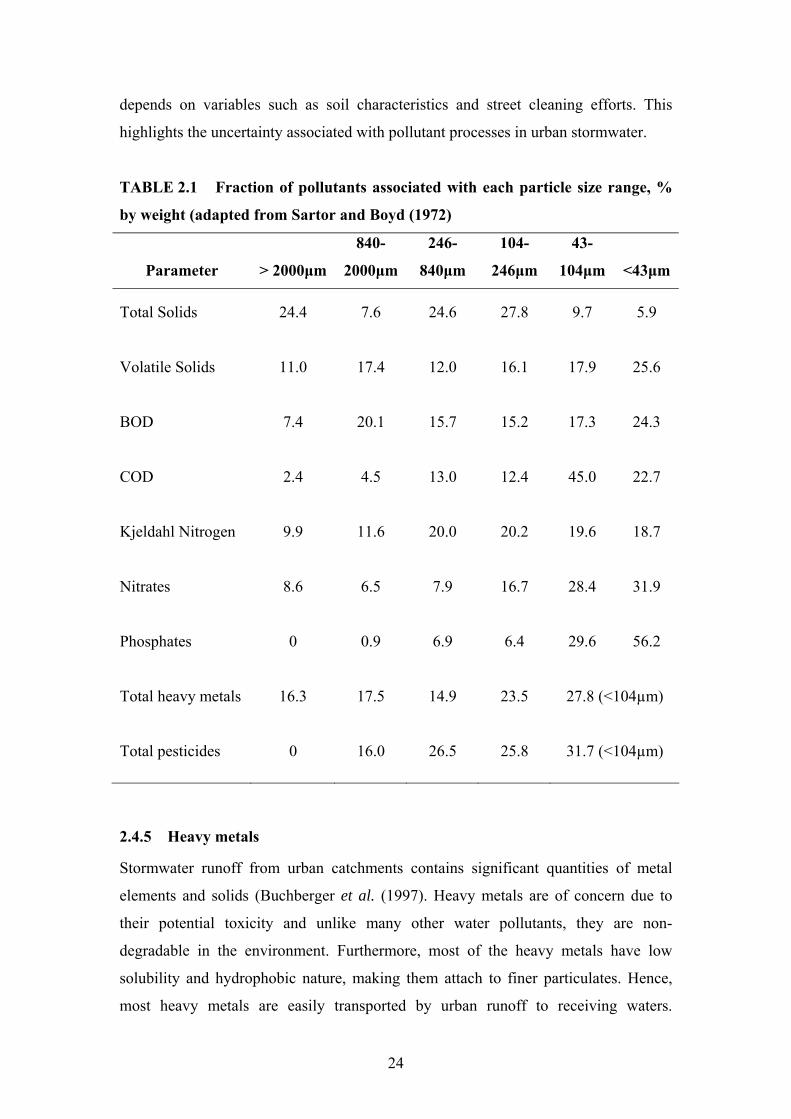
than 300μm. The conclusions by Sartor and Boyd (1972) were similar in terms of the
fraction of pollutants associated with particle sizes below 300μm at different locations
in USA, as shown in Table 2.1 below. These findings are of importance since
sediment removal procedures such as mechanical street sweeping (Bender and
Terstriep 1984) have been found to be inadequate for particles smaller than 250μm.
Gromaire et al. (2000) found that street cleaning procedures in Paris, France have
limited impact on the reduction of street runoff pollution, especially heavy metals.
Contradictory results relating to the particle size distribution of sediment in urban
runoff highlights the site-specific nature of urban stormwater pollution. Liebens
(2001), in confirming the variability of particle size distribution of urban sediments,
attributed this to land use and soil characteristics of the catchment. However, Liebens
(2001) also noted that the differences in particle size distribution between different
land uses were very small and statistically insignificant. This has been attributed to
similar soil erosion processes at the sites chosen by the researcher. Consequently,
finer particles play an important role in the transport of pollutants by runoff to
receiving waters. Nevertheless, the particle size distribution is highly site-specific and
24
depends on variables such as soil characteristics and street cleaning efforts. This
highlights the uncertainty associated with pollutant processes in urban stormwater.
TABLE 2.1 Fraction of pollutants associated with each particle size range, %
by weight (adapted from Sartor and Boyd (1972)
Parameter > 2000μm
840-
2000μm
246-
840μm
104-
246μm
43-
104μm <43μm
Total Solids 24.4 7.6 24.6 27.8 9.7 5.9
Volatile Solids 11.0 17.4 12.0 16.1 17.9 25.6
BOD 7.4 20.1 15.7 15.2 17.3 24.3
COD 2.4 4.5 13.0 12.4 45.0 22.7
Kjeldahl Nitrogen 9.9 11.6 20.0 20.2 19.6 18.7
Nitrates 8.6 6.5 7.9 16.7 28.4 31.9
Phosphates 0 0.9 6.9 6.4 29.6 56.2
Total heavy metals 16.3 17.5 14.9 23.5 27.8 (<104µm)
Total pesticides 0 16.0 26.5 25.8 31.7 (<104µm)
2.4.5 Heavy metals
Stormwater runoff from urban catchments contains significant quantities of metal
elements and solids (Buchberger et al. (1997). Heavy metals are of concern due to
their potential toxicity and unlike many other water pollutants, they are non-
degradable in the environment. Furthermore, most of the heavy metals have low
solubility and hydrophobic nature, making them attach to finer particulates. Hence,
most heavy metals are easily transported by urban runoff to receiving waters.

25
Therefore, understanding the processes governing build-up and wash-off of heavy
metals in an urban environment is of critical importance.
Heavy metals have been primarily recognised as traffic-related pollutants (Dong et al.
1984; Sansalone and Buchberger 1997; Wilber and Hunter 1979). However, a large
number of additional sources have also been listed in the literature. Table 2.2 below
lists some of the most recognised heavy metal sources in urban environments.
TABLE 2.2 Sources of heavy metals in an urban environment (Drapper et al.
2000; Sansalone et al. 1996; Vermette et al. 1991; Fergusson and Ryan 1984;
Ellis et al. 1986)
Source Pb Zn Cd Cu Ni Cr Mn Fe Al
Fuel and exhaust
Tires
Brakes
Engine wear
Vehicular component wear
Paint
Soil
Other sources of heavy metals in urban areas also include corrosion of buildings and
their appurtenances, atmospheric deposition and various industrial activities including
intentional and accidental spills (Christensen and Guinn 1979; Davis et al. 2001).
Several other sources such as fungicides and insecticides (Cu and Cd) and asphalt

26
paving (Ni) have also been found to contribute to the build-up of heavy metals in
urban areas (Ball et al. 1998).
Metals in urban stormwater runoff are partitioned between dissolved and particulate-
bound fractions. The dissolved fraction of urban stormwater runoff is defined as
metals of an un-acidified sample that pass through a 0.45μm membrane filter (APHA
1999). However, most of the heavy metals in urban stormwater runoff have been
found to be attached to suspended solids (Bodo, 1989; Dong et al., 1984). Despite the
strong relationship between heavy metals and suspended solids, the evaluation of the
dissolved fraction of the heavy metal load is important as an indicator of
bioavailability. Furthermore, parameters such as dissolved organic carbon and pH can
significantly enhance desorption of heavy metals from solids. Tai (1991) noted that
the ratio of trace metals released into the dissolved phase at pH 6 against pH 8.1 is
about 180 for Zn, 45 for Pb and 25 for Fe. Sansalone and Buchberger (1997) observed
significantly larger metal element dissolved fractions in events where the rainfall pH
was low and where the average pavement residence time were the highest. Similarly,
DOC plays a major role in partitioning of metals between soluble and particulate
fractions in stormwater (Hamilton et al., 1984). The build-up and wash-off process
kinetics of heavy metals and its influence on urban stormwater are discussed in detail
in Section 2.5.
2.4.6 Polycyclic Aromatic Hydrocarbons (PAHs)
Polycyclic aromatic hydrocarbons (PAHs) or Polynuclear aromatic hydrocarbons are
fused compounds built on benzene rings. Aromatic rings are considered fused when a
pair of carbon atoms is shared. Many PAHs possess high stability due to the benzene-
like properties. The interest in PAHs in environmental studies derives from the fact
that they have been found to give rise to acute lethal and sublethal toxic effects in
freshwater organisms at very low aqueous concentrations (Warren et al. 2003).
However, Warren et al. (2003) noted that toxicity studies have generally been carried
out under controlled conditions in laboratories, often in the absence of sediments and
other factors that might control the actual bioavailability of a compound in water. This
has resulted in limited knowledge on the effect of physico-chemical parameters on the
toxicity of PAHs. The environmentally significant PAHs range from Naphthalene
(C10H8) to Coronene (C24H8). In this range there is a large number of PAHs with

27
varying number, position and eventual chemistry of substituents on the basic aromatic
ring system (Manoli and Samara 1999). It has also been found that physical and
chemical properties, such as solubility of PAHs, vary with molecular weight. The
solubility of PAHs in water is generally low due to their hydrophobic nature. Hence,
PAHs associate mainly with particulate matter.
Due to their adverse impact, PAHs are included in the United States Environmental
Protection Agency (US EPA) and in the European Union priority list of pollutants.
The US EPA has identified 16 unsubstituted PAHs as priority pollutants as listed in
Table 2.5 below, some of which are considered to be possible or probable human
carcinogens. Hence, their distribution in the environment and potential risk to human
health has been the focus of much attention (Manoli and Samara 1999).
TABLE 2.3 Priority PAHs as listed by USEPA (adapted from Manoli and
Samara 1999)
PAH compound Benzene rings Solubility [mg/L] Kow*
Naphthalene, NAP 2 32 2300
Acenaphthene, ACE 3 3.4 21000
Acenaphthylene, ACY 3 3.93 12000
Flourene, FLU 3 1.9 15000
Anthracene, ANT 3 0.05-0.07 28000
Phenanthrene, PHE 3 1.0-1.3 29000
Flouranthene, FLA 4 0.26 340000
Benzo[a]anthracene, BaA 4 0.01 4x10⁵
Benzo[b]flouranthene, BbF 5 - 4x10⁶
Benzo[k]flouranthene, BkF 5 - 7x10⁶
Chrysene, CHR 4 0.002 4x10⁵
Pyrene, PYR 4 0.14 2x10⁵
Benzo[a]pyrene, BaP 5 0.0038 106
Dibenzo[a,h]anthracene, DbA 5 0.0005 106
Benzo[ghi]perylene, BgP 6 0.00026 107
Indeno[1,2,3-cd]pyrene, IND 6 - 5x10⁷ *Kow is an octanol/water partition coefficient

28
The most common carcinogenic PAH is Benzo[a]pyrene, BaP, which contains five
fused benzene rings. However, smaller molecular weight PAHs can undergo
decomposition and react with a number of chemicals in the environment to produce
different derivatives, which can be more toxic than the original compounds (Nicolau
et al. 1984).
Hydrophobic contaminants such as PAHs can exist in a variety of forms in water: a
freely dissolved phase, as a colloidal phase or associated with sedimentary material
(Warren et al. 2003). The distribution of PAHs between the various phases is a central
issue in terms of the fate and effects of PAHs in aquatic environments. It strongly
influences concentrations in the dissolved and particulate phase and therefore has a
strong impact on water quality. In order to understand and predict this distribution, it
is crucial to examine sediments and dissolved organic matter and its influence on the
build-up and wash-off process kinetics of PAHs (Warren et al. 2003). Section 2.6
discusses the important processes determining build-up and wash-off of PAHs in an
urban environment in detail.
2.5 Build-up and wash-off processes of heavy metals
2.5.1 Build-up
Numerous sources of metals are present in an urban environment as outlined in
Section 2.4.5. However, their quantification has been proven to be extremely difficult.
Fluctuations in build-up concentrations of heavy metals have been reported
suggesting that the input and relative importance of these sources will vary in the
urban environment (Sartor and Boyd 1972; Davis et al. 2001). These fluctuations
have been attributed to factors such as antecedent dry periods and land use
characteristics. In addition to this, variability does not appear to be affected by a
single factor but by several interacting factors. For example, Vermette et al. (1991)
noted antecedent dry days and previous street cleaning as well as wind direction
during sampling to affect build-up concentrations of heavy metals. Antecedent dry
period is important due to most heavy metals exhibiting low solubility and metal’s
affinity with sediments (Yuan et al. 2001). Nevertheless, it has been found that
despite an increase in sediment loading over the length of a monitoring period, metal

29
concentrations can stay relatively constant (Ellis et al. 1986). It can be concluded that
the antecedent dry period significantly influences the amount of accumulated particles
available for wash-off. However, the relative importance of the antecedent dry period
is highly variable and questionable in relation to the build-up of heavy metals in an
urban area.
Similarly, land use has been suggested as playing an important role in the build-up of
heavy metals. Brezonik and Stadelmann (2002) found that commercial and industrial
land uses in Minnesota USA contributed a higher amount of heavy metals than a
residential site. Similar results were found by Droppo et al. (1998) in a catchment in
Ontario USA, where total concentrations of Pb, Cu, Cd, Zn and Mn exhibited the
highest concentrations within the industrial part of the catchment. This is not
surprising since Cu, Cd, Zn and Mn have been attributed to increased industrial
industries (Vermette et al. 1991; Yun et al. 2000). For example, Robertson et al.
(2003) noted that Zn compounds were used in the manufacture of alloys, glass, dry
cell batteries and electrical equipment. High metal concentrations in commercial areas
are most likely due to an increased traffic density compared to a residential site. This
is attributed to metals such as Pb and Cr, which have been found to be strongly
dependant on site specific traffic density (Yun et al. 2000). Similarly, Shaheen (1975)
showed that close to 100% of Pb entering receiving waters originated from traffic-
related sources. However, due to the increase in the use of unleaded fuel in the last
two decades, this is questionable and should be interpreted carefully.
Liebens (2001) found that street sweepings from residential areas had higher
concentrations of most of the heavy metals compared to street sweepings from
commercial areas in Florida USA. Sartor and Boyd (1972) found industrial and
residential areas to have a higher loading of heavy metals than commercial areas. The
higher concentrations and loads of metals found in industrial and residential areas
could potentially be attributed to by-products from industrial activities, residential
buildings and garden products, which could explain the higher concentrations reported
in residential and industrial areas (Davis 2001; Ball et al. 1998).
Furthermore, one of the most common sources of Cu and Zn has been found to be
brake pad and tyre wear (Drapper et al. 2000). Hence, commercial or residential areas
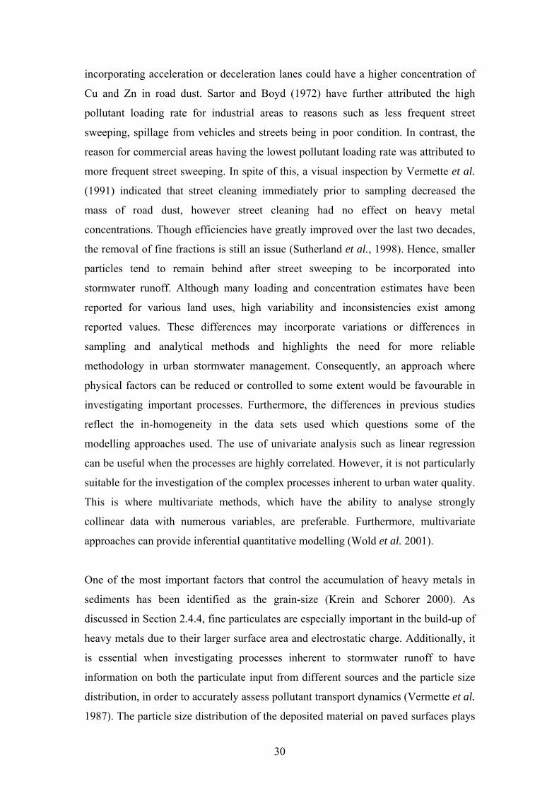
30
incorporating acceleration or deceleration lanes could have a higher concentration of
Cu and Zn in road dust. Sartor and Boyd (1972) have further attributed the high
pollutant loading rate for industrial areas to reasons such as less frequent street
sweeping, spillage from vehicles and streets being in poor condition. In contrast, the
reason for commercial areas having the lowest pollutant loading rate was attributed to
more frequent street sweeping. In spite of this, a visual inspection by Vermette et al.
(1991) indicated that street cleaning immediately prior to sampling decreased the
mass of road dust, however street cleaning had no effect on heavy metal
concentrations. Though efficiencies have greatly improved over the last two decades,
the removal of fine fractions is still an issue (Sutherland et al., 1998). Hence, smaller
particles tend to remain behind after street sweeping to be incorporated into
stormwater runoff. Although many loading and concentration estimates have been
reported for various land uses, high variability and inconsistencies exist among
reported values. These differences may incorporate variations or differences in
sampling and analytical methods and highlights the need for more reliable
methodology in urban stormwater management. Consequently, an approach where
physical factors can be reduced or controlled to some extent would be favourable in
investigating important processes. Furthermore, the differences in previous studies
reflect the in-homogeneity in the data sets used which questions some of the
modelling approaches used. The use of univariate analysis such as linear regression
can be useful when the processes are highly correlated. However, it is not particularly
suitable for the investigation of the complex processes inherent to urban water quality.
This is where multivariate methods, which have the ability to analyse strongly
collinear data with numerous variables, are preferable. Furthermore, multivariate
approaches can provide inferential quantitative modelling (Wold et al. 2001).
One of the most important factors that control the accumulation of heavy metals in
sediments has been identified as the grain-size (Krein and Schorer 2000). As
discussed in Section 2.4.4, fine particulates are especially important in the build-up of
heavy metals due to their larger surface area and electrostatic charge. Additionally, it
is essential when investigating processes inherent to stormwater runoff to have
information on both the particulate input from different sources and the particle size
distribution, in order to accurately assess pollutant transport dynamics (Vermette et al.
1987). The particle size distribution of the deposited material on paved surfaces plays

31
a critical role in urban stormwater management strategies. Larger particles are
relatively easy to monitor and remove. Fine material has the ability, when
incorporated into urban stormwater runoff, to stay in suspension longer and is
therefore transported a greater distance by urban runoff (Deletic et al. 1996). The
influence of fine particulates in heavy metal transport is discussed in detail in Section
2.5.2.
2.5.2 Wash-off
As noted in Section 2.4.5, metals transported by urban stormwater are partitioned into
a dissolved and a particulate fraction. However, the distribution of heavy metals in
urban stormwater is difficult to predict as it depends on a variety of factors associated
with anthropogenic metal input, such as pollution origin, concentration and
characteristics of suspension, colloidal and dissolved ligands and changes in physico-
chemical parameters of the water (Gueguen and Dominik 2003). It has also been
found that the longer the sediments stay in aqueous suspension, the greater the degree
of adsorption and/or desorption of pollutants, and the biological transformations of
degradable components will be more extensive (Dong et al. 1984). Generally, metal
elements in urban environments partition into dissolved and particulate-bound
fractions of runoff as a function of:
• pH
• Metal element solubility
• Solid concentration
• Origin of heavy metal pollution
• Pavement residence time
• Runoff volume
• Antecedent dry period
• Dissolved organic carbon
• Reducing conditions (mainly for Manganese (Mn) which is a redox sensitive
metal
• Chemical form
(Ellis and Revitt 1982; Hamilton et al. 1984; Sansalone and Buchberger 1997;
Sonzogni et al. 1980; Ujevic et al. 2000; Gueguen and Dominik 2003)

32
These factors underline the uncertainties in the literature in relation to different
dissolved metal concentrations and loadings noted by many researchers. For example,
Morrison et al (1984) found high levels of Cu in stormwater solids, which may be due
to the high percentage of particulate organic material recorded. Bubb and Lester
(1993) found Cu and Zn to be primarily particulate bound while Shinya et al. (2000)
found Ni to be mostly associated with the dissolved phase. Legret and Pagotto (1999)
found that Pb usually appears in the particulate form (91%) whereas the other heavy
metals investigated were usually dissolved (60% for Zn, 56% for Cu and 54% for Cd).
The association with the dissolved fraction by metals such as Cu, Zn and Ni is not
surprising since they have been found to be strongly complexed by organic ligands
(Qu and Kellermann 2001). Consequently, they may interact in solution with
dissolved organic matter, which in turn is concentrated by the adsorption to fine
particulates such as clay minerals. The association of Cd with the dissolved phase is
most likely due to its loose binding through cation exchange and easily reducible
phases. Hence, Cd, Cu and Zn are likely to be transported in the dissolved phase in
stormwater runoff and be directly bioavailable, when reaching receiving waters.
However, most of the heavy metals in urban stormwater runoff are strongly attached
to suspended solids due to their low solubility (Shinya et al. 2000; Ujevic et al. 2000).
Different metal elements will distribute differently in urban runoff. Generally, a
partition coefficient (Kp) is used to describe a metal’s affinity for sediment
interactions. Kp is defined as the ratio of the solid phase concentration (Cs) with the
aqueous phase concentration (Caq). A metal element generally has a specific Kp value
due to its specific solubility. However, a metal’s partition coefficient can vary
significantly due to the highly laboratory based studies used to develop Kp. Hence, a
number of processes in urban environments can influence the partition coefficient.
DeWitt et al. (1992) found Kp values to vary within a factor of ten when organic
matter was present in urban stormwater (DeWitt et al. 1992). This is most likely due
to chemical transformations occurring in the sediment organic matter as it is digested
and metabolized by benthic fauna and microflora. Similar results have been found in
urban stormwater in Australia by Ball (2000), where the ratio of particulate load to
total load was not consistent between three catchments investigated. The use of
partition coefficients to describe sediment interactions in field samples is further
restricted by the difficulty in obtaining aqueous samples with representative solids

33
concentration (Sansalone and Buchberger 1997). Consequently, analytical methods to
measure the concentrations of micro-pollutants are more accurate if sufficient solids
are available. Hence, measurements based on a relatively small amount of solids
could contain gross errors and bias the partition coefficient.
Metal concentrations generally increase with decreasing particle size (Liebens 2001;
Ujevic et al. 2000). This is due to the relatively large surface area of fine sediments
and their higher sorption capacity (Dong et al. 1984). The enrichment of metals on
fine particles is a major environmental problem since no efficient removal technique
for fine particles is known. Coarse particles can easily be removed by settling ponds
and street sweeping. Research has shown that street sweeping is only effective for
particles of 250μm size and larger (Bender and Terstriep 1984; Sutherland et al.
1998). Since most metals have a greater affinity for smaller particle sizes,
conventional cleaning programs would have little effect in reducing toxic runoff
levels, as fine suspended particulates are readily transported in stormwater. However,
high concentrations of heavy metals have occasionally been found in the coarse
fraction of urban street dust suggesting that a broad range of particle sizes should be
investigated for accurate results (Dong et al. 1984). Hamilton et al. (1984) suggested
that the partitioning of heavy metals in particles occur in five fractions:
• The exchangeable fraction;
• Carbonate fraction;
• Fe-Mn Oxide fraction;
• Organic fraction; and
• Residual fraction.
The exchangeable fractions are metals specifically surface bound and subject to
sorption-desorption processes due to changing ionic composition of stormwater. The
carbonate fraction, on the other hand, contains metals that are moderately available
for release to runoff but are highly susceptible to a pH change. Iron and manganese
oxides exist in road sediments as cement between particles or as surface coatings on
particles. Furthermore, metals can be irreversibly trapped in the crystal lattice of
primary and secondary minerals (Charlesworth and Lees 1999). Hamilton (1984)
found the organic fraction to play a major role in partitioning of metals in stormwater.

34
This has also been observed by Droppo et al. (1998), who found Cu to be mostly
bound within the organic fraction independent of the land use. Similarly, Ellis et al.
(1986) found increased metal levels in the organic fraction of the sediments. This is of
concern due to the enhanced toxicity that can occur in metal-organic complexation.
More importantly, the relationship between organic carbon and heavy metals could
lead to an enrichment of bioavailable metals due to microbial degradation of the
organic matter subsequently bringing the metal into solution (Ellis and Revitt 1982).
Additionally, as Charlesworth and Lees (1999) have noted, the highest proportion of
each heavy metal is bound to different particle fractions independent of particle size.
Carbonates were found to dominate in the binding of Cd, Zn and Cu while the organic
fraction dominated in binding Ni and Pb. This means that changes in the
environmental conditions could lead to the release of different heavy metals into the
water column.
2.6 Build-up and wash-off processes of PAHs
2.6.1 Build-up
The development and industrialisation over the past half-century has resulted in
organic compounds such as PAHs becoming ubiquitous in the urban environment.
Hence, their distribution and accumulation is of critical importance in urban
stormwater studies.
PAHs originate from both anthropogenic and natural sources. Some of the natural
sources of PAHs have been identified as volcanic eruptions and forest fires (Manoli
and Samara 1999; Bae et al. 2002). Savinov et al. (2000) also found that PAHs were
formed by direct biosynthesis by bacteria, fungi, higher plants and insect pigments.
However, the input from natural sources is low compared to anthropogenic sources in
urban areas. PAHs in urban environments are mainly the by-products of incomplete
combustion or pyrolysis of organic material (Van Metre et al. 2002; Grynkiewicz et
al. 2002). For example, Phenanthrene (PHE), Flouranthene (FLA) and Pyrene (PYR)
are typical by-products of diesel combustion while higher-molecular weight PAHs
such as Indeno[1,2,3-cd]pyrene (IND) and Benzo[ghi]perylene (BgP) are typical
gasoline engine by-products (Bae et al. 2002). Possible sources of PAHs may also be

35
assessed by the concentration ratios of individual PAH compounds as noted by Zhou
and Maskaoui (2003), who found that a ratio of PHE/Anthracene (ANT) smaller than
10 and a ratio of FLA/PYR larger than 1 indicated that the PAH contamination is
from combustion processes. Several other important sources listed in the literature
include:
• Oil residues;
• Sewage outfalls;
• Industrial wastewater;
• Aluminum production;
• Tyre wear; and
• Road-wear
(McCready et al. 2000; Rogge et al. 1993; Zhou and Maskaoui 2003).
Although a number of processes have been identified as major sources of PAHs in
urban areas, the input from a single source is difficult to quantify. In fact, PAHs are
often found in a wide range of concentrations, indicating that they have many
different sources. Despite their anthropogenic origin in urban areas, PAHs can occur
at relatively high concentrations in rural and remote areas due to their ability to be
transported over long distances as gases or aerosols (Manoli and Samara 1999). This
is further supported by higher molecular-weight PAHs’ apparent resistance to
biodegradation (Warren et al. 2003). Furthermore, biodegradation of lower molecular-
weight PAHs have been found to be limited in urban stormwater due to the
insufficient time for build-up of enzymes to degrade these compounds (Gavens et al.
1982).
A study by Yamane et al. (1997) found that the following factors affect the
degradation of PAHs:
• Organic and inorganic nutrient loads;
• Temperature;
• pH;
• Salinity;
• Previous chemical exposure;
• Microbial adaptations; and

36
• Existence of other PAHs.
However, the factors mentioned above are highly site specific and can differ between
ecosystems. In addition to this, due to its stability as a compound, the impact these
degradation processes have on the quality of urban stormwater is minor. Hence, a
significant amount of PAH build-up can be incorporated in urban runoff and
transported to receiving waters.
2.6.2 Wash-off
PAHs in urban runoff have been associated with particulate matter, with up to 90%
occurring in the particulate phase. Only a small fraction of their total load is generally
in the aqueous phase and considered bioavailable (Hoffman et al. 1985). This is
supported by Marsalek et al. (1997) who reported dissolved PAHs’ concentrations to
be less than 11%. However, PAHs have been detected in the dissolved phase at
concentrations above its aqueous solubility (Smith et al. 2000). It has been postulated
that this contradictory finding could be due to either the presence of colloidal-size
particles capable of sorbing PAHs to an appreciable extent, or the presence of an oil-
and-grease micro emulsion, which enhances the solubility of PAHs. Similarly, Warren
et al. (2003) noted that colloidal particles can sorb non-ionic organic pollutants and
enhance their apparent solubility in water, and thereby facilitate pollutant transport in
environmental systems. They have referred to this phenomenon as the ‘solubility
enhancement’ effect. Furthermore, the distribution of PAHs in the dissolved phase has
also been found to be a function of the type of sources available in the urban
environment (Readman et al. 1987). This is most likely due to petrogenic sources of
PAHs, such as point sources of oil and petrochemicals being dominant, which would
increase the water/sediment ratio of PAHs. PAHs originating from pyrogenic sources
such as incomplete combustion are generally attached to particulates.
PAHs are not very soluble in the water phase (Gonzalez et al. 2000; Makepeace et al.
1995; Marsalek et al. 1997; Wang et al. 2001). The solubility of PAHs in water have
been found to decrease with increasing molecular weight of the PAH (Manoli and
Samara 1999). This supports findings by Zhou and Maskaoui (2003) and McCready et
al. (2000) where the composition pattern of PAHs in sediments was mostly dominated
by high molecular-weight PAHs consisting of three or more benzene rings. Wang et

37
al. (2001) found the dominant compounds in all particle size fractions to be those with
three or more rings, accounting for 79-93% of the total PAH concentrations in each
size fraction. Hence it can be concluded that a significant amount of highly toxic, high
molecular-weight PAHs are transported by fine sediments in urban stormwater.
According to studies by Choi and Chen (1976), Zuofeng (1987) and Evans et al.
(1990), PAHs have been found to have a tendency to be associated with the silt and
clay fractions. However, Readman et al. (1984) found a decrease in PAH content of
estuarine sediment with decreasing particle size from sand to clay (100 to 10μm) and
Hoffman et al. (1984) stated that PAHs attached to particulates in stormwater had a
maxima in the 125 to 150μm range and below 45μm particle sizes. As discussed in
Section 2.4.2, organic carbon can influence the concentration and distribution of
pollutants attached to sediments. Positive correlations have been found between PAHs
and sedimentary organic carbon by several researchers. For example, Wang et al.
(2001) found a relationship between PAHs and sedimentary organic carbon in all
sediment size fractions. Based on their results, they also suggested that sedimentary
organic matter has PAH sorption characteristics. A number of studies have clearly
demonstrated the important role that organic matter plays in the adsorption of PAHs
in sediments (Gustafsson et al. 1997; Karickhoff et al. 1979; Kleineidam et al. 1999).
On the other hand, several researchers have suggested that the type and source of
organic matter is more important in the sorption of micro-pollutants than the amount
(Krein and Schorer 2000; Warren et al. 2003). Similarly, Dewitt et al. (1992) found
that the spatial and temporal variation in the bioavailability and sorption of PAHs in
water samples was more a function of the source of the dissolved organic carbon
rather than the concentration.
Simpson et al. (1998) found high PAH concentrations to be associated with large size
fractions (300-1180μm and >1180μm), which contained high particulate organic
matter. Kim et al. (1999) observed a positive correlation between PAHs and
sedimentary organic carbon. However, Maruya et al. (1996) reported high
concentrations to be associated with silt and clay fractions and suggested sedimentary
organic matter to have less effect on the distribution of PAHs in sediment. Macias-
Zamora et al. (2002) found PAH concentrations in surface marine sediments to be
correlated (r2=0.612) with organic matter content. Evans et al. (1990) suggested that

38
there are two optimal particle sizes with which organic matter becomes associated,
one between 40 and 63μm, and the other in the 500μm to 2mm size range due to
fragmentary plant material. Evans et al. (1990) also found a positive linear
relationship between organic matter and PAHs, which was similar for each sediment
size fraction. Other researchers who studied the distribution of PAHs into particles
have also found a correlation between PAHs and the organic fraction of particles
(Catallo and Gambrell 1987; Choi and Chen 1976; Readman et al. 1982).
Nevertheless, different PAH compounds have different relationships with sedimentary
organic matter due to its water solubility and the number of partitioning coefficients
that exist. As noted by Zhou et al. (1999), particle-water interactions were one of the
most important mechanisms controlling the distribution and movement of
hydrophobic organic chemicals such as PAHs in aquatic environments. To accurately
predict the transport and fate of PAHs in water, the partition coefficient Kp and the
organic carbon normalised partition coefficient Koc are widely used. The importance
of the organic carbon normalised partition coefficient Koc has been attributed to the
fact that laboratory experiments have shown that organic matter is the principal
particulate component responsible for the adsorption of hydrophobic organic
compounds such as PAHs (Zhou et al. 1999). The three most widely used coefficients
in the literature are listed below:
• Kow (octanol/water partition coefficent);
• Kp (linear partition coefficient between particles and water); and
• Koc (partition coefficient on an organic carbon basis).
However, large variations in partition coefficient values have been reported for the
same compound. In general, this variation is thought to be attributed to differences in
the nature of the organic matter that affect the partitioning of the compound. These
differences have been attributed to:
• Differences in the source and the extent of weathering of the organic matter;
• The effect of particle mineral type on the adsorption of organic matter; and
• The effect of particle mineral type on the configuration of the sorbed organic
matter
(Karickhoff et al. 1979; Warren et al. 2003).

39
In general, it would appear that less-polar organic matter gives rise to higher Koc
values than higher-polarity organic matter (Warren et al. 2003). This is most likely
due to the better hydrophobic environment in less-polar organic matter.
Differences in partition coefficient values for the same compound has also been
attributed to soot carbon content of the particulate matter (Zhou et al. 1999;
Gustafsson et al. 1997). This suggests that PAHs associated with particles could in
fact be present in the form of soot and soot-like particles and not subject to particle-
water interactions. In other words, the PAHs on soot-like particles are strongly bound
and not influenced by further partitioning between the particles and water. This would
significantly affect the speciation of PAHs. Similarly, parameters such as pH and
temperature have been found to influence the sorption characteristics and solubility of
specific PAH compounds (Warren et al. 2003). Hence, variations in the partition
coefficients of a specific PAH compound are likely to occur in urban stormwater.
Consequently, while total PAH concentration has a positive correlation with organic
carbon, the relationship between a specific PAH compound and organic carbon may
vary.
The concentrations and types of PAHs found in sediments have been shown to reflect
the source characteristics and related physico-chemical properties of individual PAHs
that influence sediment binding, such as the octanol/water partition coefficient Kow
(Kucklick et al. 1997). Herrmann (1981) concluded that the sorption behaviour of
PAHs played an important role in their transport in aqueous systems and suggested
that PAH compounds were transported by means of adsorption to suspended solids,
bedload and solution in films of mineral oil around those sorbents. Krein and Schorer
(2000) concluded that different particle sizes were transported by different hydraulic
conditions where intensity of rainfall was found to be responsible for the wash load,
and the grain size distribution to be controlled by the amount of rainfall.
2.7 Summary
Urban stormwater has been identified as one of the leading causes of the degradation
of receiving waters. Generally, this has been attributed to the generation of pollutants
by anthropogenic activities in urban areas. This has led to increased research activity

40
recent decades. Pollutant sources and pathways have been clearly identified in the
literature.
The primary water pollutants identified in the literature include:
• suspended solids;
• nutrients;
• organic carbon;
• heavy metals; and
• hydrocarbons.
Heavy metals and PAHs are of major concern in urban runoff due to their toxicity and
stability as compounds. In addition, numerous PAHs have been recognised as
carcinogenic and acutely toxic to aquatic organisms. Both PAHs and heavy metals
have been identified as primarily traffic-related pollutants. However, numerous
sources such as industrial activities and atmospheric deposition can contribute an
appreciable amount of PAHs and heavy metals to urban areas. The significance of
suspended solids and organic carbon stems from the fact that PAHs and heavy metals
are influenced by numerous chemical processes inherent to suspended solids and
organic carbon characteristics. This primarily relates to the adsorption of PAHs and
heavy metals to fine particles, due to their increased organic matter content and
relatively larger surface area compared to coarse particles. This could have serious
implications for urban stormwater management strategies due to the increased
difficulty in removing pollutants attached to fine particles. Furthermore, a number of
processes such as microbial degradation of the organic matter and the presence of
colloidal particles can significantly influence the bioavailability of PAHs and heavy
metals in urban stormwater.
The processes underlying the build-up and wash-off processes of pollutants have been
difficult to determine. This has primarily been attributed to the limited understanding
of the interactions between various influential parameters in urban water quality.
Consequently, relationships that have been developed have been far from satisfactory
and have led to limited transferability of the results. Furthermore, the influence of
chemical processes on the build-up and wash-off of pollutants have generally been

41
neglected in previous research due to research methodologies being largely based on
physical factors. Hence, the lack of control of physical factors to determine the
influence of chemical and physico-chemical processes in urban water quality has
significantly constrained the outcomes. Therefore, a multi disciplinary approach is
preferable and techniques and methodologies commonly used in agricultural and
chemical research could be successfully implemented. This is primarily attributed to
control of rainfall characteristics and the use of appropriate statistical tools. Hence, an
approach to urban water quality research using rainfall simulation could significantly
enhance the research outcomes and facilitate transferability of relationships found due
to the increased control of physical factors. Furthermore, common modelling
approaches used in urban water quality studies have been linear regression or similar
univariate techniques. However, as identified in the literature, the processes inherent
to urban water quality are complex. Hence, multivariate methods which can handle
incomplete and noisy data with many variables and observations are a more powerful
approach for the analysis of complicated problems.

42
Chapter 3 Design and Fabrication of a Rainfall Simulator
3.1 Introduction
Chapter 2 clearly identified the difficulties encountered in the use of natural rainfall
events in urban water quality research. This was primarily attributed to high
variability in rainfall intensity, non-uniformity of rainfall associated with the use of
large heterogenous areas and lack of control of physical factors in urban water quality
studies. Moreover, the complexity of the processes involved in urban stormwater
requires a reliable database. As Ahyerre et al. (1998) noted, the processes governing
build-up and wash-off of pollutants in urban areas are very complex, as they concern
many media, space and time scales. Additionally, the random nature of the occurrence
and characteristics of natural rainfall introduces further variables into a research arena
where so little of the inherent processes are known. Therefore, the use of artificial
rainfall can help to eliminate significant constraints such as dependency on natural
rainfall experienced by researchers undertaking rigorous research into urban
stormwater quality. Furthermore, rainfall simulation can significantly enhance the
transferability of the research, due to the reduction and control of physical variables
usually inherent to urban water quality research.
The use of rainfall simulators to produce artificial rainfall to generate databases for
urban water quality research is rarely adopted. Conversely, rainfall simulators have
been seen as important tools in agricultural research, such as erosion and infiltration
studies on runoff plots (Grierson and Oades 1977; Loch et al. 2001; Meyer and
McCune 1958). It was imperative to find an equally efficient tool for urban water
quality research. This chapter identifies the characteristics needed for successful
simulation of rainfall on paved surfaces. It also describes the design criteria used for
the development of a rainfall simulator suitable for the research project and how it
was applied in urban water quality research.
3.2 Design of a rainfall simulator
The function of a rainfall simulator is highly dependant on the desired outcome of the
individual research. As Meyer (1988) noted, rainfall simulators need to be designed
and calibrated accurately for the conditions in which they are to be used. Therefore,

43
characteristics used in the design of previous rainfall simulators needed to be
interpreted carefully and re-assessed to fit the needs of the individual research.
Previous rainfall simulators have primarily focused on agricultural research such as
erosion studies. Thus, the rainfall simulators used have been designed specifically for
this purpose. However, there are a number of rainfall simulator design characteristics
from agricultural research that are applicable to urban water quality studies. Moore et
al. (1983) noted that the general criteria for rainfall simulation, independent of the
focus of the study should be:
• Rainfall characteristics;
• Plot size; and
• Portability and construction/operation cost.
More detailed criteria were as follows:
• Drop-size distribution near to that of natural rainfall;
• Drop impact velocities near to that of natural rainfall;
• Uniform rainfall intensity and drop size distribution over the entire plot;
• Rainfall application nearly continuous over the entire plot;
• Reproducible storm patterns of durations and intensities of interest;
• No efficiency losses when used under field conditions, such as high temperature
and moderate winds;
• Plot area adequate to represent the treatments and conditions being examined;
• Highly portable, including: (a) disassembled portability for easy movement from
site-to-site; and (b) assembled portability for easy movement from plot-to-plot at a
given location; and
• Low cost in construction and operation
(Bubenzer 1979a; Bubenzer 1979b; Hall 1970; Meyer 1979; Meyer and McCune
1958; Moore et al. 1983).
The majority of the criteria mentioned above were applicable to rainfall simulation on
paved surfaces such as the reproduction of physical characteristics of rainfall and
portability of the rainfall simulator. However, many of the previous rainfall simulator

44
studies were not consistent with the focus of this research. Thus, the rainfall simulator
developed for this research was designed to meet the following primary requirements:
• complete portability, easy assembly and operation;
• drop-size distribution, terminal velocity and kinetic energy similar to natural
rainfall in the region;
• ability to reproduce the chemical characteristics of natural rainfall in the region;
• ability to create rainfall intensities suitable for the proposed research study;
• small homogenous plot area to reduce the number of inherent variables;
• ability to apply rainfall uniformly over the plot area; and
• satisfactory system for runoff collection from paved surfaces.
Considerable design and development were necessary to ensure that the rainfall
simulator met the research requirements outlined above. The different stages involved
in the design and development process are discussed below. The system developed for
the collection of wash-off samples is described in Section 4.4. Only an introduction to
the sample collection system will be discussed here.
3.2.1 Re-production of natural rainfall characteristics
One of the most important criteria for the developed rainfall simulator was the ability
to accurately reproduce natural rainfall characteristics, both physical and chemical.
Hence, both the chemical and physical profile of rainfall in the region had to be
studied.
(A) Physical Characteristics
The rainfall simulator developed in this research used three Veejet 80100 nozzles to
reproduce natural rainfall characteristics. A number of different nozzles were
available commercially with different characteristics and spray patterns. However, as
noted by Meyer and McCune (1958), nozzles used for rainfall simulation should have
either square or fan spray pattern, as illustrated in Figure 3.1, in order to obtain
acceptable intensity, drop-size, drop velocity and distribution characteristics.

45
FIGURE 3.1 Fan spray pattern nozzle (adapted from www.spray.com)
Nozzle orifice diameter and the pressure of the water entering the nozzle determine
the characteristics noted above (Assouline et al. 1997). Generally, an increase in
pressure generates a smaller drop size from the nozzle. A high discharge nozzle such
as the Veejet 80100 was therefore preferable to obtain drop-sizes and velocities near
natural rainfall. Furthermore, the Veejet 80100 nozzle was chosen due to its median
drop size of 2 1/8 mm diameter (Meyer and McCune 1958), which was similar to the
median drop size in natural rainfall at intensities lower than 160mm/hr (Hudson
1963). The kinetic energy has been calculated as 29.49J/m2mm on the basis of
measured drop-size and velocity (Loch et al. 2001). Similar kinetic energy was
reported for natural rain in South-East Queensland at intensities above 40mm/hr
(Rosewell 1986). Hence, the Veejet 80100 nozzle satisfied all the physical rainfall
characteristics set out in the research. However, the Veejet 80100 nozzle may not
completely replicate the characteristics of natural rainfall as noted by Morin et al.
(1967). Though better than other known nozzles, it has been found that the nozzle
only provides 80% of the kinetic energy per unit volume of rain. Moreover, rainfall
characteristics have regional differences and while the kinetic energy and drop-size
distribution from a Veejet 80100 nozzle provided the most reliable simulation of
natural rainfall, it is important to note that natural rainfall characteristics were very
difficult to reproduce completely.
The pressure used in this research was 41 kPa which has been commonly applied to
the Veejet nozzle 80100 in past rainfall simulation research (Bubenzer and Meyer
1965; Loch et al. 2001; Meyer and Harmon 1979). This was due to the drop size
distribution, impact velocity and kinetic energy of the simulated rainfall being similar
to natural rainfall with intensities over 25mm/hr at the specific pressure for the Veejet
80100 nozzle.

46
Due to the Veejet 80100 nozzle being a high-discharge nozzle, producing an intensity
of about 580mm/hr when spraying continuously over a plot (Moore et al. 1983), a
technique to lower the intensity had to be adopted. Intermittent rainfall spraying was
therefore employed, which has been used successfully in numerous rainfall simulator
studies (Floyd 1981; Grierson and Oades 1977; Moore et al. 1983). Pulsed rainfall
application, such as intermittent rainfall, did not affect the characteristics obtained
(Loch et al. 2001). In fact, rainfall is highly intermittent by nature. Furthermore, the
fan spray pattern of the Veejet 80100 nozzle demanded it to be moved perpendicular
to the long dimension of the spray pattern to cover a greater area during rainfall
(Meyer and McCune 1958). Hence, an oscillating nozzle boom sweeping the plot area
had to be introduced. Oscillating nozzles have been used extensively in rainfall
simulation (Bubenzer and Meyer 1965; Floyd 1981; Loch et al. 2001).
Oscillation of nozzles has been carried out primarily by oscillation of a boom driven
by a small motor, with the nozzles being fixed to the boom (Foster et al. 1979; Loch
et al. 2001; Moore et al. 1983). A similar system was used for the rainfall simulator
developed in this research, which is described in the hydraulic and control systems
sections (Sections 3.2.3 and 3.2.4 respectively). Rainfall intensity applied to the
designated plot area was varied by changing the cycle time of the oscillating nozzles
as described by Loch et al. (2001). Overspray troughs and return pans were required
to collect excess nozzle discharge when rainfall was not applied to the plot area, and
to limit the spray on the plot to near vertical, which is described in Section 3.2.2. The
choice of angle of spray was determined by the height of the nozzle boom and the size
of the designated runoff plot as discussed in Sections 3.2.2 and 3.2.5 respectively. The
nozzles sprayed an area larger than the runoff plots to ensure that the raindrop splash
was the same into the runoff plot as it was out of the runoff plot, which is further
discussed in Section 3.2.5.
(B) Chemical profile
In order to re-produce natural rainfall characteristics in the area as closely as possible,
the chemical quality of rainfall in the study region was investigated by collecting
natural rainfall. Rainwater collected in tanks was not considered due to the risk of
unwanted pollutants, particularly if obtained from metal roofs. Consequently, 23
rainwater samples were collected over a period of 30 days and a rainfall quality
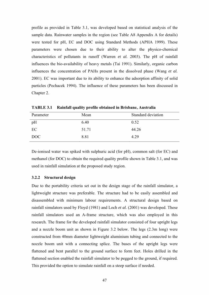
47
profile as provided in Table 3.1, was developed based on statistical analysis of the
sample data. Rainwater samples in the region (see Table A8 Appendix A for details)
were tested for pH, EC and DOC using Standard Methods (APHA 1999). These
parameters were chosen due to their ability to alter the physico-chemical
characteristics of pollutants in runoff (Warren et al. 2003). The pH of rainfall
influences the bio-availability of heavy metals (Tai 1991). Similarly, organic carbon
influences the concentration of PAHs present in the dissolved phase (Wang et al.
2001). EC was important due to its ability to enhance the adsorption affinity of solid
particles (Pechacek 1994). The influence of these parameters has been discussed in
Chapter 2.
TABLE 3.1 Rainfall quality profile obtained in Brisbane, Australia
Parameter Mean Standard deviation
pH 6.40 0.52
EC 51.71 44.26
DOC 8.81 4.29
De-ionised water was spiked with sulphuric acid (for pH), common salt (for EC) and
methanol (for DOC) to obtain the required quality profile shown in Table 3.1, and was
used in rainfall simulation at the proposed study region.
3.2.2 Structural design
Due to the portability criteria set out in the design stage of the rainfall simulator, a
lightweight structure was preferable. The structure had to be easily assembled and
disassembled with minimum labour requirements. A structural design based on
rainfall simulators used by Floyd (1981) and Loch et al. (2001) was developed. These
rainfall simulators used an A-frame structure, which was also employed in this
research. The frame for the developed rainfall simulator consisted of four upright legs
and a nozzle boom unit as shown in Figure 3.2 below. The legs (2.3m long) were
constructed from 40mm diameter lightweight aluminium tubing and connected to the
nozzle boom unit with a connecting splice. The bases of the upright legs were
flattened and bent parallel to the ground surface to form feet. Holes drilled in the
flattened section enabled the rainfall simulator to be pegged to the ground, if required.
This provided the option to simulate rainfall on a steep surface if needed.
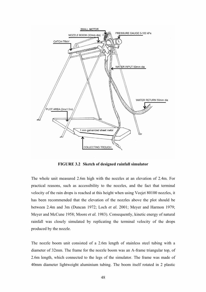
48
FIGURE 3.2 Sketch of designed rainfall simulator
The whole unit measured 2.6m high with the nozzles at an elevation of 2.4m. For
practical reasons, such as accessibility to the nozzles, and the fact that terminal
velocity of the rain drops is reached at this height when using Veejet 80100 nozzles, it
has been recommended that the elevation of the nozzles above the plot should be
between 2.4m and 3m (Duncan 1972; Loch et al. 2001; Meyer and Harmon 1979;
Meyer and McCune 1958; Moore et al. 1983). Consequently, kinetic energy of natural
rainfall was closely simulated by replicating the terminal velocity of the drops
produced by the nozzle.
The nozzle boom unit consisted of a 2.6m length of stainless steel tubing with a
diameter of 32mm. The frame for the nozzle boom was an A-frame triangular top, of
2.6m length, which connected to the legs of the simulator. The frame was made of
40mm diameter lightweight aluminium tubing. The boom itself rotated in 2 plastic

49
bushes, which also prevented lateral movement of the boom. The three Veejet 80100
nozzles were spaced 1m apart on the nozzle boom. A sketch of the nozzle boom is
shown in Figure 3.3 below.
FIGURE 3.3 Cross section of the nozzle boom unit
The water supply inlet was via a 38mm flexible hose attached to the nozzle boom
opposite to the row of nozzles. A pressure gauge (0-100 kPa) was fitted to the water
supply inlet so that the operating pressure could be monitored at nozzle height. A
water pressure of 41 kPa was always present in the nozzle boom during simulation
and the nozzles were producing continuous water flow throughout operation. Flow not
required as rainfall on the test surface was recycled via catch trays made of stainless
steel sheets running on either side of the 2.6m long nozzle boom as shown in Figure
3.4. During operation, the nozzles oscillated through approximately 95o. Of this
travel, the middle 55o applied raindrops onto the runoff plot, while the remaining 40o
was used at either end of the travel for overlap into the catch trays as shown in Figure
3.5. Adjusting the frequency and speed of nozzle oscillation altered the rainfall
intensity of the simulated rainfall. Calibration and performance details of the rainfall
simulator are provided in Section 3.3. The catch trays were connected to the return
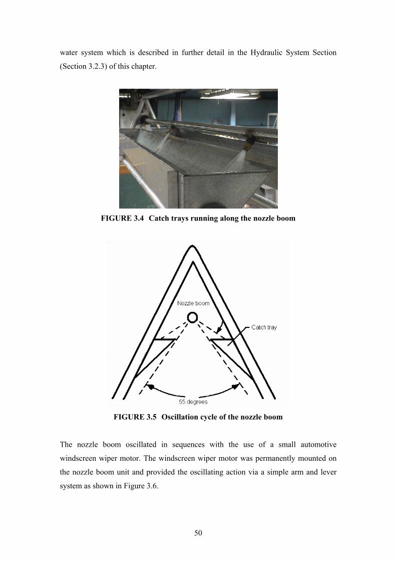
50
water system which is described in further detail in the Hydraulic System Section
(Section 3.2.3) of this chapter.
FIGURE 3.4 Catch trays running along the nozzle boom
FIGURE 3.5 Oscillation cycle of the nozzle boom
The nozzle boom oscillated in sequences with the use of a small automotive
windscreen wiper motor. The windscreen wiper motor was permanently mounted on
the nozzle boom unit and provided the oscillating action via a simple arm and lever
system as shown in Figure 3.6.

51
FIGURE 3.6 Arm and lever system oscillating the nozzle boom
Similar small motor systems have been used successfully in oscillating nozzle booms
on previous rainfall simulators (Floyd 1981, Loch and Foley 1992). Loch et al. (2001)
used a stepper motor for the oscillation of the nozzles. However, the advantages of a
stepper motor compared to a windscreen wiper motor were minimal. The only
advantage was the ability to drive at the same speed in both directions. This would
have minimal impact on simulating natural rainfall characteristics however, since
rainfall is intermittent by nature. Consequently, the oscillation of the nozzle boom
provided by a small windscreen wiper motor was adequate. A control box, which is
further explained in the Oscillation Control System Section (Section 3.2.4), was used
to control the speed and delay of the oscillation.
3.2.3 Hydraulic System
Water was supplied to the rainfall simulator by a general transfer pump (Grundfos
CH2-30) connected to a Honda 12 Ampere petrol generator. The pump transferred
water from a 200L reservoir to the nozzle boom. The pump and reservoir were
connected with a 38mm diameter flexible hose and two 40mm cam-locks at either
end. A mesh filter was fitted between the reservoir and pump which, prevented
clogging in the pump system. The pump-reservoir unit was permanently mounted on a
conventional trailer (1.8x1.2m), which is described in Section 3.2.6. When needed,
the reservoir was topped up from a 1000L reservoir carried to the field.

52
A 40mm cam-lock connected the pump to the water delivery line, which consisted of
a 4m section of 38mm diameter flexible hose. Another 40mm cam-lock connected the
water delivery line to the nozzle boom. The discharge rate was controlled by a gate
valve at the outlet of the pump and measured by the water pressure entering the nozzle
boom, as indicated by the pressure gauge installed at nozzle boom level. Catch trays
on either side of the nozzle boom were used to collect water from the nozzles not
spraying on the runoff plot as shown in Figure 3.4. Water collected in the catch trays
during rainfall simulation was gravity fed via a 50mm flexible hose back to the 200L
reservoir for reuse.
3.2.4 Oscillation Control System
The oscillation control system consisted of a controller box with circuits controlling
the speed and delay of the automotive windscreen wiper motor, which in turn
controlled the oscillation cycle of the nozzle boom. The controller box could be
switched on and off by a toggle switch on the side. By changing the speed and delay
of the nozzles sweeping over the plot, rainfall intensity could be controlled. The speed
was controlled by a variable speed control switch with six speed settings, which
increased and decreased the speed of the windscreen wiper operating the oscillation of
the nozzle boom. Similarly, the delay was controlled by a variable delay switch
increasing and decreasing the time (0-12s) between oscillation cycles. The controller
box was powered by a rechargeable 12V battery. During field operation of the rainfall
simulator, the battery was recharged using the Honda generator providing power to
the general transfer pump. The control system was calibrated as described in Section
3.3, so that specific settings on the speed and delay switches represented specific
rainfall intensities.
3.2.5 Runoff plot and collection
The runoff plot dimensions (2x1.5m) were chosen after the calibration of the
discharge patterns of the nozzles mounted on the nozzle boom as discussed in Section
3.3. The plot was enclosed by a frame sealed to the ground by rubber flaps, tape and
silicone as discussed in Section 4.4. A specially designed collection trough was
attached to the frame at the bottom of the plot, as can be seen in Figure 3.2 and further
evaluated in Section 4.4. The runoff water collected in the trough was vacuumed into
25L drums by a commercially available vacuum cleaner system. The runoff collection

53
system and its calibration is described in Section 4.4 and will not be discussed further
here.
3.2.6 Storage and Transport
A 1.8x1.2m box trailer was used for storing and transporting the rainfall simulator
from site to site. The trailer held a Honda 12 Ampere petrol generator with
rechargeable 12V battery as well as a 200L water reservoir. The reservoir was
connected to the permanently mounted Grundfos general transfer pump on the bed of
the trailer. The legs and the nozzle boom unit of the rainfall simulator were mounted
on trailer racks and secured with elastic straps to the trailer when stored or
transported. The trailer with the rainfall simulator is shown in Figure 3.7 below. An
additional 1000L water reservoir was carried to the field by an additional vehicle,
where it was used to top up the 200L reservoir when needed.
FIGURE 3.7 The rainfall simulator fully mounted on the box trailer
3.3 Performance calibration of the rainfall simulator
The rainfall simulator was carefully designed to reproduce natural rainfall
characteristics as closely as possible. However, the design was based purely on
theory. Hence, it was unknown how well the rainfall simulator would simulate design
rainfall characteristics in the field. Furthermore, a number of control box settings
needed to be calibrated to represent design rainfall intensities in the area prior to the
rainfall simulator being used in field work. Therefore, parameters such as intensity,

54
uniformity of rainfall and drop size distribution needed to be calibrated in order to
accurately replicate the design rainfall characteristics.
3.3.1 Nozzle discharge and pattern
Initially, twelve nozzles of the Veejet 80100 series were obtained for testing for their
suitability for rainfall simulation. However, only three nozzles were to be mounted on
the nozzle boom. The nozzles were therefore chosen based on their performance in
terms of discharge and spray pattern created by an individual nozzle under 41kPa
water pressure. The nozzles with the most similar spray patterns were then chosen.
The discharge rate was measured using a container held under the nozzle for a period
of time, ranging from 10 to 40 seconds. The average discharge in litres per minute
(L/min) was calculated by weighing the collected water. The temperature of the water
used was measured between each run to accurately determine the density to be used in
each discharge rate calculation. The average discharge rates for each nozzle are shown
in Figure 3.8. As can be seen, the nozzles investigated had an average discharge rate
varying between 13.88L/min and 15.11L/min. The mean discharge rate based on all
twelve nozzles was 14.37±0.32L/min. Nozzles 2, 8 and 11 were determined to be
unsuitable to use in rainfall simulation due to their large deviation from the mean
discharge rate.
FIGURE 3.8 Average discharge rates for the twelve Veejet 80100 nozzles (41kPa
pressure)
13.2 13.4 13.6 13.8
14 14.2 14.4 14.6 14.8
15 15.2
Dis
char
ge ra
te [L
/min
]
1 2 3 4 5 6 7 8 9 10 11 12
Nozzle no
Discharge rate for Veejet 80100 nozzles
Mean discharge

55
The spray pattern of the remaining nine nozzles was investigated in order to determine
which nozzles could be incorporated into the rainfall simulator. Thirty two (32)
containers with an opening of 85mm diameter spaced 300mm apart, as illustrated in
Figure 3.9, were placed underneath a nozzle, which was mounted on the nozzle boom
2.4m high. The containers were exposed to nozzle spray for a time period of five
minutes and the collected water was weighed and converted into a volume
measurement.
FIGURE 3.9 Calibration of spray pattern of the nozzles
The contour of each nozzle was then plotted using the spacing of the containers and
the percentage of total water volume collected in each container. Based on the
findings from the spray pattern investigations, nozzles 3, 4 and 12 were chosen to be
used in rainfall simulation. The spray contours of the three chosen nozzles are shown
in Figure 3.10. A higher value indicates a higher percentage of the total rainfall
recorded over the plot.

56
FIGURE 3.10 Nozzle spray pattern contours for the chosen nozzles (3, 4 and 12
respectively)
3.3.2 Rainfall intensities and uniformity of rainfall
Intensity measurements were carried out by using a row of closely placed containers
and measuring the volume accumulated during a known time interval as described by
Lascelles et al. (2000) and Loch et al. (2001). The volume of water collected in the
containers was converted to rainfall depth per hour (mm/hr). In this instance a row of
seven containers was placed underneath the three nozzles, as shown in Figure 3.11,
and was exposed to simulated rainfall for five minutes.
FIGURE 3.11 Intensity measurements using seven containers

57
The oscillation (speed and delay) settings of the control box were varied for each run,
which gave a reasonable replication of the range of rainfall intensities that could be
simulated. Initial intensity measurements served as platforms in choosing a number of
speed and delay settings suitable for rainfall simulation. Three different speed settings
and eight different delay settings were initially investigated as shown in Table 3.2
below.
TABLE 3.2 Calculated average rainfall intensities using seven containers for
different speed and delay settings of the control box
Speed setting number Delay [s] Average rainfall intensity [mm/hr]
4 1 184
4 2 149
4 5 82
4 6 65
4 8 57
4 10 45
3 1 148
3 2 108
3 3 79
3 5 59
3 6 52
3 8 41
3 10 36
3 12 32
2 1 159
2 2 107
2 3 75
2 5 52
2 6 47
2 8 41
2 10 35
2 12 28

58
The calculated rainfall intensities for the different settings were in the range of 28-
184mm/hr. Due to a number of control box settings not being investigated, the
complete range of rainfall intensities produced by the rainfall simulator is unknown.
However it is postulated, from calibration results, that rainfall intensities as low as 10-
15mm/hr and as high as 220mm/hr can be simulated using the rainfall simulator.
Nevertheless, the rainfall intensities obtained from the initial calibration using seven
containers is highly overestimated for the plot area to be investigated due to end
effects. In fact, a much larger area of containers had to be investigated to be able to
find average intensities for each setting. Therefore, six settings were chosen (intensity
range 47-148mm/hr) for further investigation. The settings investigated were:
• Speed setting 2, delay 2s (Initial intensity 107mm/hr);
• Speed setting 2, delay 3s (Initial intensity 75mm/hr);
• Speed setting 2, delay 6s (Initial intensity 47mm/hr);
• Speed setting 3, delay 1s (Initial intensity 148mm/hr);
• Speed setting 3, delay 1.5s (No initial intensity measured); and
• Speed setting 3, delay 5s (Initial intensity 59mm/hr).
The average intensity of the settings was measured by placing 77 containers in a grid
pattern (7x11) under the nozzles, as shown in Figure 3.12. The spacing between each
container was 230mm in both directions across the plot, making up a grid of
containers 1465mm wide and 2385mm long.

59
FIGURE 3.12 Container grid pattern used for calculating average rainfall
intensity produced by the rainfall simulator
The containers were exposed to five minutes of simulated rainfall for each of the six
settings. The volume of water in each container was then recorded (data provided in
Table A1-A6 Appendix A) and average rainfall intensity over the plot was calculated.
It was found that the initial calculation of rainfall intensities for the different settings
was overestimated due to rainfall depth at the ends of the plot being lower compared
to the rainfall depth at the middle of the plot. Hence, a new set of intensities were
calculated for the different settings. These were:
• Speed setting 2, delay 2s (Average intensity 86mm/hr);
• Speed setting 2, delay 3s (Average intensity 65mm/hr);
• Speed setting 2, delay 6s (Average intensity 43mm/hr);
• Speed setting 3, delay 1s (Average intensity 133mm/hr);
• Speed setting 3, delay 1.5s (Average intensity 115mm/hr); and
• Speed setting 3, delay 5s (Average intensity 54mm/hr);
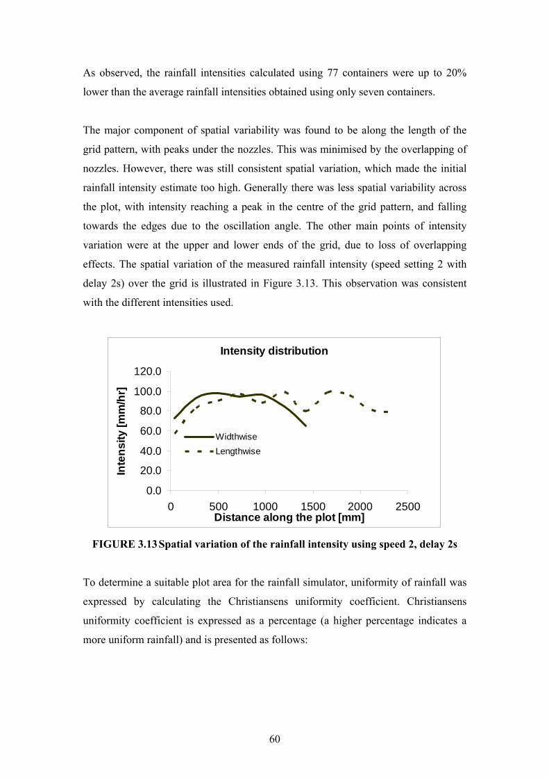
60
As observed, the rainfall intensities calculated using 77 containers were up to 20%
lower than the average rainfall intensities obtained using only seven containers.
The major component of spatial variability was found to be along the length of the
grid pattern, with peaks under the nozzles. This was minimised by the overlapping of
nozzles. However, there was still consistent spatial variation, which made the initial
rainfall intensity estimate too high. Generally there was less spatial variability across
the plot, with intensity reaching a peak in the centre of the grid pattern, and falling
towards the edges due to the oscillation angle. The other main points of intensity
variation were at the upper and lower ends of the grid, due to loss of overlapping
effects. The spatial variation of the measured rainfall intensity (speed setting 2 with
delay 2s) over the grid is illustrated in Figure 3.13. This observation was consistent
with the different intensities used.
Intensity distribution
0.0
20.0
40.0
60.0
80.0
100.0
120.0
0 500 1000 1500 2000 2500Distance along the plot [mm]
Inte
nsity
[mm
/hr]
WidthwiseLengthwise
FIGURE 3.13 Spatial variation of the rainfall intensity using speed 2, delay 2s
To determine a suitable plot area for the rainfall simulator, uniformity of rainfall was
expressed by calculating the Christiansens uniformity coefficient. Christiansens
uniformity coefficient is expressed as a percentage (a higher percentage indicates a
more uniform rainfall) and is presented as follows:
61
)1(100nmx
Cu ×−×= ∑ (Christiansen 1942)
Where: Cu = uniformity coefficient
m = mean value
n = number of observations
x = deviation of individual observation from mean
A uniformity coefficient of above 80% is considered to be sufficient in successful
rainfall simulation (Loch et al. 2001). However, uniformity coefficients up to 95%
have been reported by researchers when end rows of the runoff plot are excluded
(Lascelles et al. 2000).
Uniformity coefficients (Cu) were calculated for the entire grid pattern used,
(1465x2385mm) as well as when the end longitudinal rows were excluded, which
made the dimensions of the plot 1465x1925mm, in order to determine the best
possible plot area. The uniformity coefficients calculated for the different intensities
are shown in Table 3.3.
TABLE 3.3 Uniformity Coefficients (Cu) for the intensities investigated
Cu [%]
Intensity [mm/hr]
Total grid
(1465x2385mm)
End longitudinal rows
excluded (1465x1925mm)
43 82.6 86.3
54 82.6 86.8
65 82.3 86.6
86 83.1 89.1
115 83.0 87.0
133 83.4 87.5
As expected, the uniformity coefficients increased when the end longitudinal rows
were excluded from the calculation due to the decreased rainfall depth recorded in the

62
end rows. Hence, the plot area chosen was 1500x2000mm due to the improved
rainfall uniformity. No significant pattern in Cu could be observed when the intensity
was changed, which suggests that changing the speed and delay settings of the rainfall
simulator had limited effect on the uniformity of rainfall.
The final intensities obtained, as shown in Table 3.3, were matched with a number of
design rainfall (ARI) events to be simulated in the field. Twelve events based on four
different intensities were selected from design rainfall for Brisbane using the
methodology given in Australian Rainfall and Runoff (Institution of Engineers 2001).
Hence, four of the six intensities calibrated were adequate to satisfy the number of
rainfall intensities to be used in the research project. The design rainfall events chosen
are shown in Table 3.4.
TABLE 3.4 Design rainfall events selected
Event Intensity [mm/hr] Duration [min]
1 year ARI 65 20
1 year ARI 86 10
1 year ARI 115 5
2 year ARI 65 35
2 year ARI 86 20
2 year ARI 115 10
2 year ARI 133 7
5 year ARI 133 13
10 year ARI 65 65
10 year ARI 86 40
10 year ARI 115 25
10 year ARI 133 17
3.3.3 Calibration of drop size and kinetic energy
The final calibration step used to determine the characteristics of simulated rainfall
and compare it to natural rainfall characteristics in the area was the measurement of
the median drop size and the approximate kinetic energy of the simulated rainfall.
Due to the water pressure reaching the nozzles being constant, the ARI events listed in

63
Table 3.4 had the same drop size distribution over the plot. Similarly, due to drop size
distribution being constant, the kinetic energy of the twelve ARI events was identical.
The two most widely used methods for the direct measurement of the diameter of
water drops are to cause the individual drops to form stains on an absorbent material
such as blotting paper, or to form pellets when collected in a powder material such as
flour or cement (Hudson 1963; Assouline et al. 1997). The method chosen to
determine the median drop size of the rainfall simulator at a water pressure of 41kPa
was the flour pellet method developed by Hudson (1963). This was primarily due to
technical difficulties of the stain method, such as establishing the relationship between
the size of the drop and size of stain and the variations in this relation due to different
degrees of splashing by large and small drops and variations in absorbency of the
sampling medium. However, it is important to note that the flour pellet method was
influenced by several factors, including the degree of compaction of the flour and the
height of fall. The method developed by Hudson (1963), and later used by Lascelles
(2000), was followed as closely as possible in order to accurately determine the
median drop size of the rainfall simulator.
A tray (diameter 240mm) of uncompacted flour was exposed to simulated rainfall for
a period of two seconds. Following exposure, the flour was dried for 12 hours at 105o
C and the pellets formed were passed through a nest of sieves as shown in Figure
3.14. The sizes of the sieves were:
• 4.75mm;
• 3.35mm;
• 2.36mm;
• 1.18mm;
• 0.6mm; and
• 0.5mm.
The mass of each pellet represented a mass ratio (drop mass/pellet mass) such that
every pellet could be converted to a corresponding rain drop according to the data
provided by Hudson (1963). The calculated median raindrop size (d50) was 2.1mm,
which was similar to values obtained by several previous researchers using 41kPa
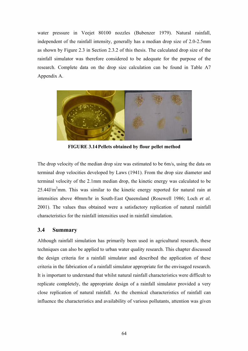
64
water pressure in Veejet 80100 nozzles (Bubenzer 1979). Natural rainfall,
independent of the rainfall intensity, generally has a median drop size of 2.0-2.5mm
as shown by Figure 2.3 in Section 2.3.2 of this thesis. The calculated drop size of the
rainfall simulator was therefore considered to be adequate for the purpose of the
research. Complete data on the drop size calculation can be found in Table A7
Appendix A.
FIGURE 3.14 Pellets obtained by flour pellet method
The drop velocity of the median drop size was estimated to be 6m/s, using the data on
terminal drop velocities developed by Laws (1941). From the drop size diameter and
terminal velocity of the 2.1mm median drop, the kinetic energy was calculated to be
25.44J/m2mm. This was similar to the kinetic energy reported for natural rain at
intensities above 40mm/hr in South-East Queensland (Rosewell 1986; Loch et al.
2001). The values thus obtained were a satisfactory replication of natural rainfall
characteristics for the rainfall intensities used in rainfall simulation.
3.4 Summary
Although rainfall simulation has primarily been used in agricultural research, these
techniques can also be applied to urban water quality research. This chapter discussed
the design criteria for a rainfall simulator and described the application of these
criteria in the fabrication of a rainfall simulator appropriate for the envisaged research.
It is important to understand that whilst natural rainfall characteristics were difficult to
replicate completely, the appropriate design of a rainfall simulator provided a very
close replication of natural rainfall. As the chemical characteristics of rainfall can
influence the characteristics and availability of various pollutants, attention was given

65
to reproduce both the physical and chemical quality of rainfall in the study region as
closely as possible.

66
Chapter 4 Study Areas and Sampling Procedure
4.1 Introduction
The build-up and wash-off process kinetics of PAHs and heavy metals were
investigated for three different land uses in the Gold Coast region in Queensland,
Australia. The influence of land use characteristics and the related anthropogenic
activities on pollutant loadings and concentrations have been investigated by
numerous researchers (for example Sartor and Boyd 1972; Liebens 2001; Hoffman et
al. 1984). However, the outcomes reported are sometimes conflicting and have
limited reliability. As Brezonik and Stadelmann (2002) found when developing
multiple linear regression models on stormwater data from 15 different studies
encompassing 68 different catchments, the most accurate predictions were found to be
where sites were grouped according to land use. On the other hand, Lopes et al.
(1995) observed no statistically significant relationship between land use and
pollutant concentrations for a study in Arizona, USA. Hence, the relationships
developed have been site specific due to the heterogeneity of large catchments and the
dependency on numerous physical factors.
The rainfall simulator described in Chapter 3 used a homogenous area in order to
decrease the number of variables that could influence pollutant concentrations. Thus,
more reliable relationships could be created based on chemical processes, instead of
being influenced by physical factors. Furthermore, chemical processes influencing
pollutant build-up and wash-off were considered to be similar at different land uses,
which would increase the transferability of quantitative relationships developed
through this research. Three different land uses, namely residential, industrial and
commercial were chosen as study sites in order to confirm this hypothesis. The study
involved collecting build-up and wash-off samples in the field using the rainfall
simulator and the analysis of the samples collected. This chapter describes the study
sites chosen and the key attributes for choosing these sites. The sampling techniques
developed for dry and wet sampling in the field and the transport and treatment of the
samples collected from the study areas are also discussed.

67
4.2 Study site selection
Pollutant concentrations have been found to vary significantly between commercial,
industrial and residential areas (Sartor and Boyd 1972; Droppo et al. 1998). However,
it is hypothesised that build-up and wash-off process kinetics are relatively unaffected
by the pollutant concentration available. Consequently, the land use characteristics of
each site was not considered a governing factor in the build-up and wash-off process
kinetics of PAHs and heavy metals, but rather the different land uses would determine
the types of pollutants present of paved surfaces. Hence, sites incorporating typical
characteristics for these land uses were chosen to investigate the build-up and wash-
off process kinetics of PAHs and heavy metals in order to develop reliable and
predictive relationships.
Prior to selecting the study sites, criteria were developed in order to identify the most
appropriate sites for investigation. These were:
• Fair to good street surface condition;
• Good accessibility for the use of rainfall simulation;
• Minimal disturbance to local traffic; and
• Sufficient slope for gravity flow of runoff generated from simulated rainfall.
Furthermore, for the purpose of this research, the residential site had to be in a typical
suburban area incorporating detached family houses with small gardens. The
industrial site had to have a wide range of industries and the commercial site, a
reasonably high commercial activity and vehicle movements.
4.3 Project area
The Gold Coast region is located just south of Brisbane, which is the capital city of
Queensland, Australia. The region is a popular tourist destination, with an estimated
12% of the population being visitors. The beaches, in particular, are a major tourist
attraction. Gold Coast is Australia’s sixth largest City Council with a population of
approximately 455 000 people. The Gold Coast region has a sub-tropical climate with
the majority of its precipitation occurring during the summer months December-
February. The region is 5490 km2 in extent and encompasses three major rivers, the
Pimpama, Coomera and Nerang Rivers, all flowing into the Gold Coast Broadwater as

68
shown in Figure 4.1. There are also numerous other waterways in the catchment that
together cover 7% of the total land area. Natural vegetation occupies a large
percentage of the region. However, high density urban areas are located on the east
coast of the region offering water-side living for residents. This intensive urban
development on waterways provides a direct route for urban runoff that can include a
variety of pollutants. The popularity of the area is reflected in its rapid population
growth, which is one of the highest in the state of Queensland.

69
FIGURE 4.1 Map of Gold Coast region (Not to scale)

70
4.3.1 Residential site
A number of possible research sites with residential characteristics were investigated
prior to the selection of a specific site. All of the investigated residential sites were in
the Nerang area (see Figure 4.1). Descriptions of the different sites are listed in Table
4.1 below.
TABLE 4.1 Description of possible residential research sites
Name of site Characteristics
Travis Lane Steep slope, surface in good condition, access road, no
vegetation, small width of road, medium block size
Millswyn Crescent Steep to mild slope, surface in good condition, fair
vegetation, well established area, medium block size
Woolmere Street Fair slope and surface, close to highway, frequent traffic, not
much vegetation, small width of road, large blocks
Piccadilly Lane Steep slope, fair surface, no vegetation, large blocks, high
traffic flows, access poor, space for simulation poor
Lancaster Court Mild slope, surface fair to rough, small blocks, far from
highway, poor access for simulation, noise concerns
The residential site chosen was based on the criteria listed in Section 4.2. The site was
on an access road (Millswyn Crescent shown in Figure 4.2 below) located in a typical
suburban residential area (Residential A) with detached family houses with an
approximate block size of 700 m2.
FIGURE 4.2 Residential research site (Millswyn Crescent)

71
Millswyn Crescent was chosen due to its typical suburban characteristics and the fact
that rainfall simulation could be successfully carried out without disturbing the traffic
operating at the site. The slope of the road surface (2.5% or 25m/km) was sufficient
for gravity flow of the runoff created by the rainfall simulator. Additionally, the width
of the road (approximately 7m) was sufficient to close off one lane while field studies
were undertaken. Hence, the residents of the site were minimally disturbed by the
field work. The road system is primarily used by the residents for access, which was
reflected in the relatively satisfactory condition of the street surface.
The texture depth of the street surface was measured to be 0.27mm (fine texture),
using the sand patch test described by Waters (1993) where a quantity of glass beads
was pre-weighed in the laboratory before application to the road surface. The road
surface was cleaned with a firm bristled brush in order to remove all loose material
before application of the glass beads. The beads were spread using a ruler in a radial
fashion to form a circle. The diameter of the circle was then measured and related
back to the texture depth of the surface. The diameter was measured at four places to
produce a mean diameter. The texture depth of the paved surface was used only as a
classification and identified the potential for the scouring of particles accumulated on
the surface.
An early investigation of the households at Millswyn Crescent suggested that various
chemicals were used as fertilizers or for other uses and therefore could be
incorporated into the wash-off from the area. It was also found that street sweepers
operate in the area every six weeks, which may influence the availability of pollutants
on the road surface at certain times.
4.3.2 Industrial site
Similar to the residential site, a number of possible sites were investigated prior to the
selection of the selected site (Stevens Street). The sites and their characteristics are
listed in Table 4.2.

72
TABLE 4.2 Description of possible industrial research sites
Name of site Characteristics
O’Shea Drive Timber and sheet metal industries, light slope, medium to rough
surface, good access, close to highway, dust from timber
industry high
Lawson Road Not many industries, steep slope, fair surface, bushland close,
highway close, disturbance to traffic with simulation
Palings Court Medium slope, fencing, furnishing, welding, coating, rough
surface, close to highway, traffic problem, vegetation
Stevens Street Painter, furniture, sheet metal, welding, boat builder, steep slope,
rough surface, good access, disturbance minimal
As outlined in Section 4.2, there was a need for a wide range of industries at the site,
which narrowed the search down to two possible sites (Stevens Street and Palings
Court). Stevens Street was chosen due to the minimal disturbance and better
accessibility when compared to the Palings Court site. Additionally, Stevens Street
had a sufficient slope for gravity flow of wash-off from rainfall simulation and a road
width of approximately 10m, which meant that only one lane of the road needed to be
closed during rainfall simulation. Consequently, the disturbance by the presence of the
field equipment was minimal in the area. The Stevens Street site, shown in Figure 4.3,
was on an access road to a light industrial area. A wide range of industries are located
along the road, which had an average slope of 3% (30m/km).
FIGURE 4.3 Industrial research site (Stevens Street)
The street surface condition compared to the residential site was significantly
degraded, which indicated that heavy traffic regularly operate at the site. The road

73
surface had a texture depth of 0.53mm (medium texture). It is postulated that a higher
amount of pollutants could be embedded in the surface voids at the industrial site
compared to the residential site due to the coarse texture. Hence, the rainfall intensity
could be important in loosening particles from the surface. Similar to the residential
site, street sweepers operate in the area every six weeks, which would release particles
embedded in the voids, making them available for wash-off at the next rainfall event.
4.3.3 Commercial site
A shopping centre in the region was selected as a suitable site representing a
commercial land use. This was primarily attributed to the frequent vehicle movement.
Early investigations showed that field work on access roads to shopping centres
would significantly disturb the traffic. Therefore, it was decided that rainfall
simulation would be performed in the parking lot of the shopping centre. The criteria
set out in Section 4.2 still applied to the selection of an appropriate research site. The
commercial sites considered for the study are listed in Table 4.3.
TABLE 4.3 Description of possible commercial research sites
Name of shopping
centre Characteristics
Robina Town Centre Large car park area, hard to get close to shops without
disturbing traffic, mild slope, even distribution of pollutants
questionable, very good access
Centro Nerang Fair slope, rough surface, car park, close to highway, good
access, busy parking lot
Highland Park
Centre
Mild slope, light commercial, fair surface, light traffic, poor
access
Helensvale Shopping
Centre
Poor access, parking lot, light commercial, fair traffic, medium
rough surface, medium to mild slope
The commercial research site, selected on the basis of the criteria outlined in Section
4.2 was the Centro Nerang (shown in Figure 4.4), located in very close proximity to a
major motorway, suggesting that vehicular pollutants from the traffic on the highway
could contribute to the pollutant concentrations at the site. It was noted that Centro
Nerang is located in close proximity to the Nerang River, which could potentially

74
influence the pH and EC of the soil surrounding the site due to the saline nature of the
river. Hence, particles eroded from local soils at the site could have an increased or
decreased adsorption affinity for hydrophobic pollutants. As noted by Tai (1991) a
change in the pH of stormwater could significantly influence the amount of heavy
metals in the dissolved phase.
FIGURE 4.4 Commercial research site (Centro Nerang)
Centro Nerang had 570 parking spaces and is considered to be one of the busiest
shopping centres in the region, with 45 specialty retailers in the complex. The parking
lot spaces were approximately 3x3m and were on a slope to the shopping centre itself.
Average slope of the study area was 4% (40m/km), which was sufficient for runoff
simulation. It was unknown how frequently the parking lot was cleaned using street
sweepers or similar equipment. The condition of the parking lot surface was found to
be good, but with a coarse texture, having a texture depth of 0.92mm. The coarse
texture suggested that large numbers of particles would be embedded within the voids.
Hence, the efficiency of street cleaning efforts could be significantly degraded
compared to the industrial and residential sites.
4.4 Vacuum collection system
In water quality research projects, collection of street deposit material is commonly
carried out using one of two different methods or a combination of the techniques.
These techniques are:
• Brushing/Sweeping; and
• Vacuuming
(Robertson et al. 2003; Bris et al. 1999).

75
Brushing or carefully sweeping the road surface for street deposit material has
generally been carried out when fine particulates are less important for the study.
Robertson et al. (2003) noted that sweeping or brushing the road surface is preferable
when coarser particulate sizes are favoured. Similarly, the technique used by Mahler
et al. (2004), where street deposit material was collected by scraping the surface with
a metal paint scraper, would bias coarser particle collection. As Bris et al. (1999)
noted, due to the uneven distribution between fine and coarse particulate collection
using sweeping and brushing techniques, sampling using a vacuum cleaner is
preferable. This is particularly important in urban stormwater studies since the
majority of micro-pollutants such as PAH and heavy metals are distributed in the fine
fraction of the particulates (Andral et al. 1999; Sartor and Boyd 1972). Consequently,
a vacuum system was preferable for the research undertaken and was used in the
collection of build-up samples at the study sites.
4.4.1 Selection of Vacuum Cleaner
Both industrial and domestic type vacuum cleaners have been used successfully in
previous research. Tai (1991) suggested that domestic vacuum cleaners were more
efficient in capturing fine particulates due to a finer exhaust filter when compared to a
heavy duty industrial type vacuum cleaner. Tai (1991) found that the domestic
vacuum cleaner he used recovered 96.4% of the street dirt smaller than 74μm. On the
other hand, Shaheen (1975) used an industrial type vacuum cleaner for collecting
street dust and dirt and the recovery rate was 95.3% for particles less than 45μm.
These contradictory findings suggest that the type of vacuum cleaner might be less
important than the model of the vacuum cleaner. Hence, the selection of vacuum
cleaner for this research project was based on particle collection and retention
efficiency as well as portability and power requirements of the model.
The vacuum cleaner selected was a Delonghi Aqualand model (for specifications see
Figure A1 Appendix A), which incorporated a water filtration technique as well as a
High Efficiency Particulate Air (HEPA) filter to ensure minimal escape of fine
particles through the exhaust system. The vacuum cleaner could also be powered in
the field by a generator, as described in Chapter 3. In addition, the vacuum cleaner
could be easily stored during transport to and from the study sites, which made it

76
highly portable. The water filter technique used by the vacuum cleaner is illustrated in
Figure 4.5 below.
FIGURE 4.5 Delonghi Aqualand water filter system
The water filter captured the dust, thus preventing it from being released back into the
air. As no dust-bag was used, the appliance always functioned to its maximum suction
power (1500W) which made it reliable in the field. Due to the particles retained being
suspended once vacuumed, the sample had to be separated prior to further analysis,
which is described further in Chapter 5. However, the performance of a water filter
system was deemed superior, compared to a conventional exhaust filter system, due to
its excellent retention efficiency of sub-micron particles (99.9% of particles less than
0.3μm) as per the manufacturer’s technical specifications (refer to Figure A1
Appendix A).
To further enhance particle collection, a brush-head was fitted at the end of the hose
of the vacuum cleaner. This enabled the finer fraction of street dust and dirt to be
removed from the asphalt surface during the vacuum sweeps, which enhanced the
collection of finer particles. Similar techniques have been used successfully in
previous research by Butler et al. (1992) and Bris et al. (1999). As noted by Bris et al.
(1999), the finer fraction of street dust and dirt can be more strongly bound to the
asphalt surface than the coarser fraction. Therefore, a combination of brushing and
vacuuming would introduce less bias in sampling and collect a representative urban
street dust sample.
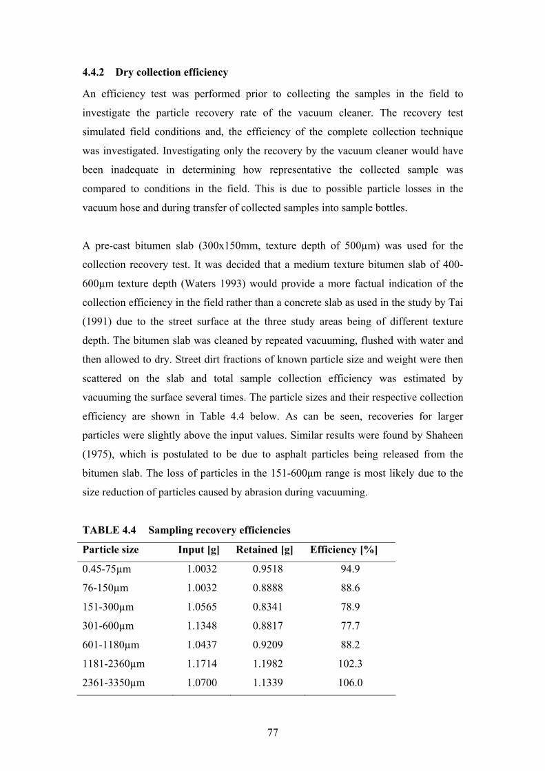
77
4.4.2 Dry collection efficiency
An efficiency test was performed prior to collecting the samples in the field to
investigate the particle recovery rate of the vacuum cleaner. The recovery test
simulated field conditions and, the efficiency of the complete collection technique
was investigated. Investigating only the recovery by the vacuum cleaner would have
been inadequate in determining how representative the collected sample was
compared to conditions in the field. This is due to possible particle losses in the
vacuum hose and during transfer of collected samples into sample bottles.
A pre-cast bitumen slab (300x150mm, texture depth of 500µm) was used for the
collection recovery test. It was decided that a medium texture bitumen slab of 400-
600µm texture depth (Waters 1993) would provide a more factual indication of the
collection efficiency in the field rather than a concrete slab as used in the study by Tai
(1991) due to the street surface at the three study areas being of different texture
depth. The bitumen slab was cleaned by repeated vacuuming, flushed with water and
then allowed to dry. Street dirt fractions of known particle size and weight were then
scattered on the slab and total sample collection efficiency was estimated by
vacuuming the surface several times. The particle sizes and their respective collection
efficiency are shown in Table 4.4 below. As can be seen, recoveries for larger
particles were slightly above the input values. Similar results were found by Shaheen
(1975), which is postulated to be due to asphalt particles being released from the
bitumen slab. The loss of particles in the 151-600μm range is most likely due to the
size reduction of particles caused by abrasion during vacuuming.
TABLE 4.4 Sampling recovery efficiencies
Particle size Input [g] Retained [g] Efficiency [%]
0.45-75µm 1.0032 0.9518 94.9
76-150µm 1.0032 0.8888 88.6
151-300µm 1.0565 0.8341 78.9
301-600µm 1.1348 0.8817 77.7
601-1180µm 1.0437 0.9209 88.2
1181-2360µm 1.1714 1.1982 102.3
2361-3350µm 1.0700 1.1339 106.0
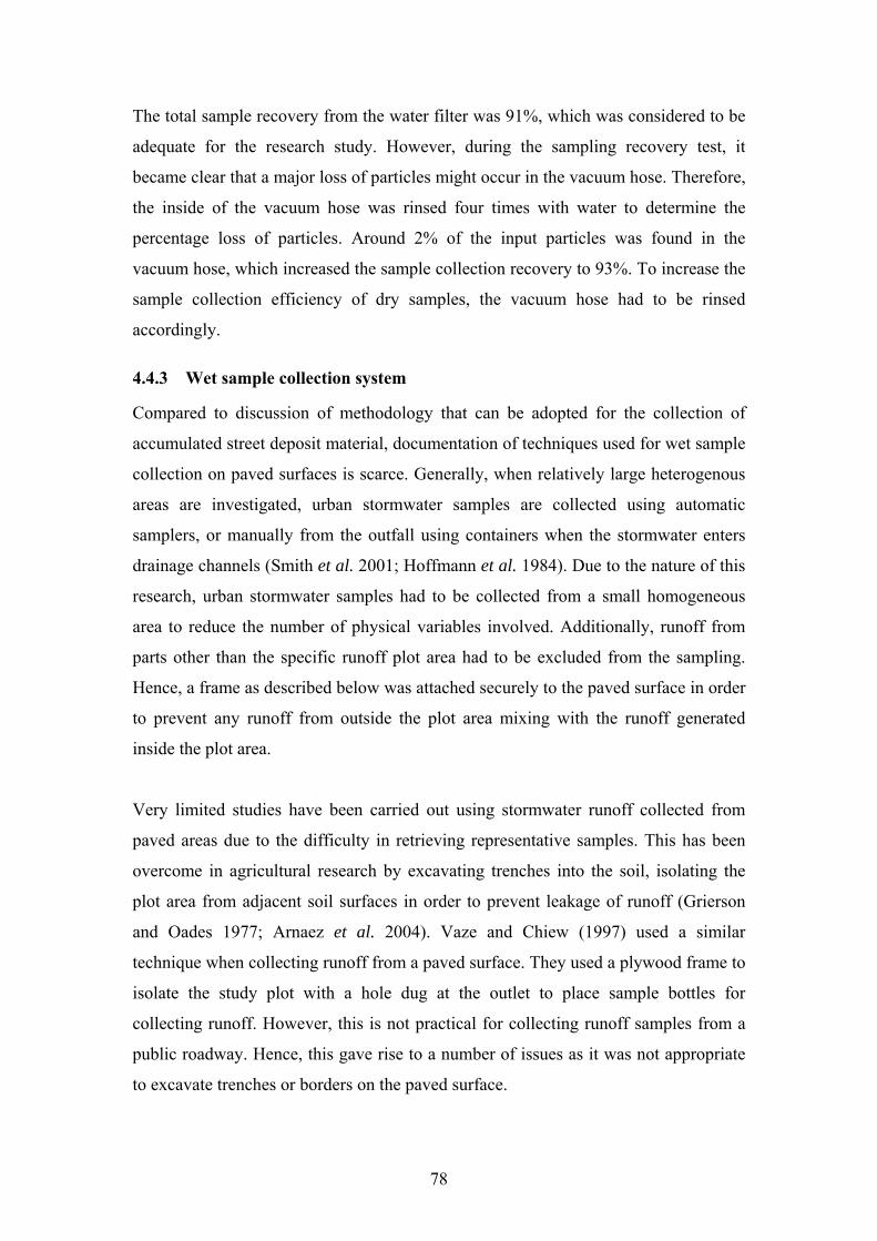
78
The total sample recovery from the water filter was 91%, which was considered to be
adequate for the research study. However, during the sampling recovery test, it
became clear that a major loss of particles might occur in the vacuum hose. Therefore,
the inside of the vacuum hose was rinsed four times with water to determine the
percentage loss of particles. Around 2% of the input particles was found in the
vacuum hose, which increased the sample collection recovery to 93%. To increase the
sample collection efficiency of dry samples, the vacuum hose had to be rinsed
accordingly.
4.4.3 Wet sample collection system
Compared to discussion of methodology that can be adopted for the collection of
accumulated street deposit material, documentation of techniques used for wet sample
collection on paved surfaces is scarce. Generally, when relatively large heterogenous
areas are investigated, urban stormwater samples are collected using automatic
samplers, or manually from the outfall using containers when the stormwater enters
drainage channels (Smith et al. 2001; Hoffmann et al. 1984). Due to the nature of this
research, urban stormwater samples had to be collected from a small homogeneous
area to reduce the number of physical variables involved. Additionally, runoff from
parts other than the specific runoff plot area had to be excluded from the sampling.
Hence, a frame as described below was attached securely to the paved surface in order
to prevent any runoff from outside the plot area mixing with the runoff generated
inside the plot area.
Very limited studies have been carried out using stormwater runoff collected from
paved areas due to the difficulty in retrieving representative samples. This has been
overcome in agricultural research by excavating trenches into the soil, isolating the
plot area from adjacent soil surfaces in order to prevent leakage of runoff (Grierson
and Oades 1977; Arnaez et al. 2004). Vaze and Chiew (1997) used a similar
technique when collecting runoff from a paved surface. They used a plywood frame to
isolate the study plot with a hole dug at the outlet to place sample bottles for
collecting runoff. However, this is not practical for collecting runoff samples from a
public roadway. Hence, this gave rise to a number of issues as it was not appropriate
to excavate trenches or borders on the paved surface.

79
The rainfall simulator applied artificial rainfall to an approximate area of 4x3m. In
spite of this, the highest uniformity of distribution was within an approximate area of
2x1.5m directly underneath the nozzles as shown in Chapter 3. Hence, the runoff plot
was defined accordingly. Furthermore, it was assumed that any escape of water due to
splash from rain drops hitting the paved surface inside a 2x1.5m runoff plot was equal
to any water entering the runoff plot due to splash outside the designated plot. A PVC
frame of 2x1.5m and 50mm high was chosen as a plot border. Rubber flaps were fixed
to the bottom of the frame to prevent water from entering or escaping the runoff plot.
The runoff plot frame with rubber flaps is shown in Figure 4.6 below.
FIGURE 4.6 Runoff plot frame used when collecting stormwater samples
The frame was attached to a specially designed collection trough from where the
runoff water was sampled. The collection trough was made out of 1mm thick
galvanised sheet metal and was placed at the outlet of the runoff plot. The collection
trough had an opening 1.5m wide so that it fitted perfectly to the width of the plot
frame. The collection trough could hold 30L of runoff water at any given time. Figure
4.6 shows the frame connected to the runoff trough. The top of the collection trough
was equipped with a handle that opened the half of the collection trough enabling the
user to collect runoff as shown in Figure 4.7 below. The runoff entering the collection
trough was collected using the same vacuum cleaner described above.
Rubber flaps

80
FIGURE 4.7 Collection trough with handle to open top for easy sampling using
the vacuum cleaner
However, some modifications had to be made to the wet vacuum system due to the
limited amount of runoff water that could be collected in the vacuum cleaner tank. A
25L high-density container was mounted between the vacuum cleaner and the suction
head. Hence, the vacuum cleaner provided the required suction, whilst the runoff was
collected separately. Thus, the runoff was collected continuously throughout an event.
Additional containers were used for large volume events. The sampling system
fabricated for wash-off is shown in Figure 4.8 below.
FIGURE 4.8 Wet sample collection system showing the connection between the
25L container and the vacuum cleaner
Prior to the collection of wash-off samples at the three sites, the wet collection system
efficiency had to be determined. An initial investigation was undertaken using only

81
the rubber flaps to enclose the runoff plot frame and the collection trough to the
ground. By visual inspection it was found that the runoff collection efficiency was
fairly low due to the amount of water leaking between the frame and the paved
surface. Hence, additional measures were necessary to enhance collection efficiency.
It was found that the corners connecting the runoff plot frame to the collection trough
were critical points of water escaping the plot. Therefore, cloth tape and a small
amount of silicone sealant was applied to the corners and let dry for an hour before
any water was applied to the plot. Cloth tape was also applied between the rubber
flaps and the ground surface all around the runoff plot frame. The combined
application of cloth tape and silicone sealant was found to be effective in preventing
leakage.
4.5 Dry sample collection in the field
Accumulated material on paved surfaces was collected using the vacuum cleaner at
the three study sites described in Section 4.4. Small asphalt surface test plots (2x1.5m)
were chosen at each of the three sites. At the residential and industrial sites, the plots
were located in the centre between the kerb and the middle strip of the road. At the
commercial site, the test plot was placed in the exact middle of a parking space. Prior
to collection, the vacuum cleaner was carefully cleaned using de-ionized water and
physical characteristics such as slope of the paved surface and length of antecedent
dry period or the last street cleaning event prior to sampling were recorded. The test
plots were then vacuumed using the vacuum cleaner as shown in Figure 4.9.
FIGURE 4.9 Dry sample collection in the field

82
The asphalt surface was vacuumed four times and the built-up material was collected
in the water filter. De-ionized water was used in the water filter of the vacuum cleaner
in order to minimise any chemical reactions with the collected particles.
Following vacuuming of the street surfaces, suspended build-up material was
transferred from the water filter and vacuum hose to sample bottles. Care was taken to
ensure that the loss of material during transfer was minimal. According to Standard
Methods for Water and Wastewater (APHA 1999), sample bottles have to be chosen
carefully, depending on the chemical analysis to be undertaken. The guidelines
provided by APHA (1999) were followed and polyethylene and amber glass bottles
were used for sample storage. Glass amber bottles were used for samples to be
investigated for PAHs, while polyethylene bottles were used for all other chemical
and physical analysis of the samples as specified by APHA (1999).
4.6 Wet sample collection in the field
Four different runoff plots were selected at each site using the same procedure as for
the selection of the build-up sampling plots. The slope of each plot was measured
using a theodolite prior to rainfall application. Although past research has shown that
a large fraction of the sediments is located near the kerb (Sartor and Boyd 1972), the
percentage distribution of heavy metals and PAHs in different particle sizes was
assumed to be the same throughout the width of the road. At the commercial site, four
parking spaces were chosen as runoff plots. The spacing between each runoff plot was
kept to a minimum without any interference occurring between the plots. Due to only
one build-up sample being collected at each site, the amount of street-deposited
pollutants was assumed to be the same for all four individual plots at each site. Hence,
the pollutant availability was considered to be identical for the rainfall events
simulated at the study sites.
Collection efficiencies of the wash-off sampling system were calculated whilst
sampling at the three study sites. The amount of rainfall sprayed on the surface was
determined from the pre set intensities and durations discussed in Chapter 3. The
volume of runoff was also recorded for each rainfall event. Hence, the volume

83
collected divided by the volume of rainfall applied to the plot became the collection
efficiency. The collection efficiencies at each site are shown in Table 4.5.
The low collection efficiency for a number of events at the commercial site was due to
a small natural rainfall event wetting the surface at the time. Even though every effort
was made to ensure the paved surface was dry, the moisture on the surface combined
with the coarse texture depth observed at the site, made it difficult to seal the interface
between the collection trough and the road surface. However, as the decrease in
collected runoff would only affect the pollutant load, it was assumed that the pollutant
concentrations would not be significantly influenced by the volume of runoff
collected. It was also assumed that some water was lost due to infiltration and
evaporation. Nevertheless, the impact of these phenomena was considered to be
minimal. As can be seen in Table 4.5, three events at the residential site and one event
at the industrial site could not be simulated due to unforeseen problems.
TABLE 4.5 Runoff collection efficiencies
Event
ARI/duration
Residential site
[%]
Industrial site
[%]
Commercial site
[%]
1yr/5min 76.9 88.0 38.3
1yr/10min 96.5 90.0 93.0
1yr/20min No data 85.4 36.9
2yr/7min 60.7 94.2 96.7
2yr/10min 72.9 87.3 40.0
2yr/20min 97.0 93.8 90.7
2yr/35min No data 85.6 35.1
5yr/13min 62.6 96.8 100
10yr/17min 75.1 97.3 100
10yr/20min 92.9 No data 33.4
10yr/40min 97.0 91.1 84.3
10yr/65min No data 82.5 34.6
Figure 4.10 shows the use of the rainfall simulator and collection of runoff samples in
the field.
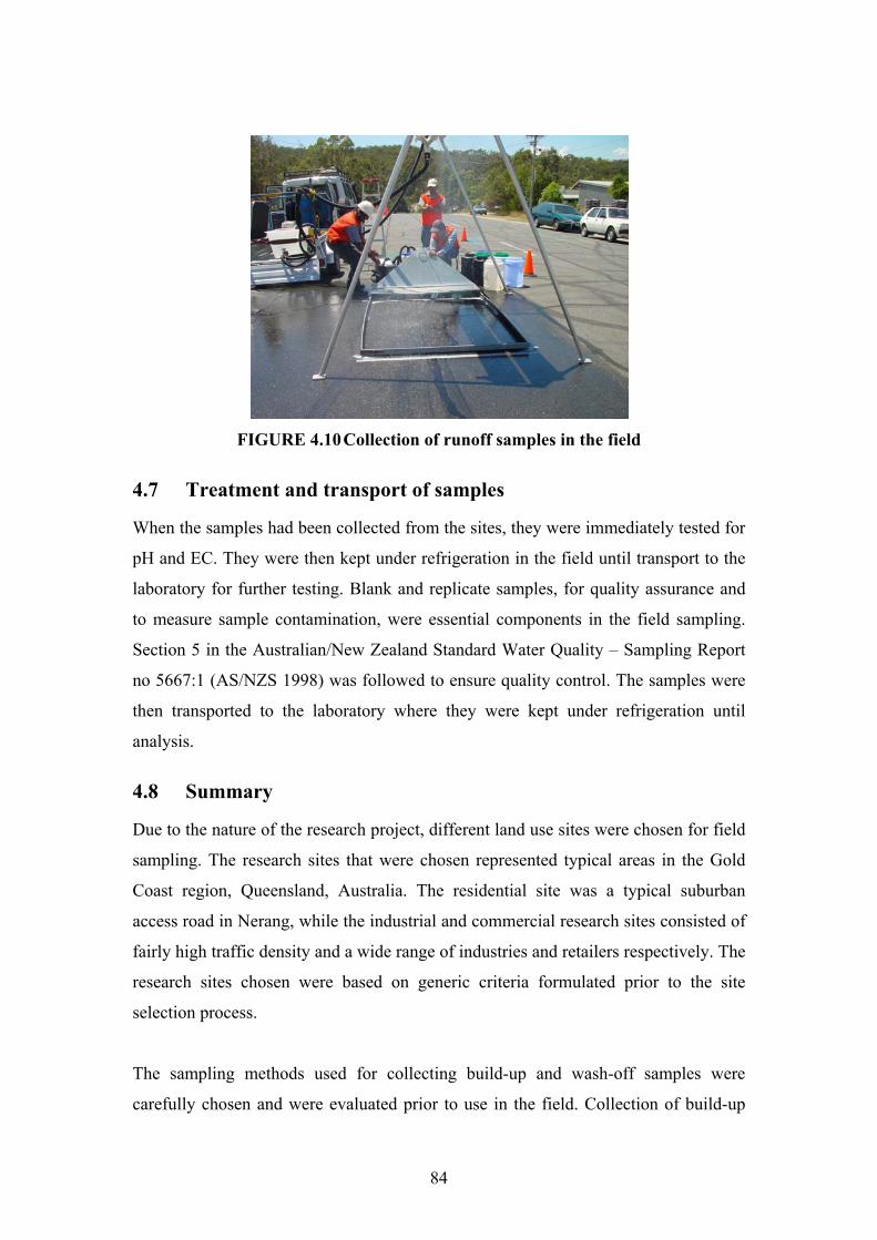
84
FIGURE 4.10 Collection of runoff samples in the field
4.7 Treatment and transport of samples
When the samples had been collected from the sites, they were immediately tested for
pH and EC. They were then kept under refrigeration in the field until transport to the
laboratory for further testing. Blank and replicate samples, for quality assurance and
to measure sample contamination, were essential components in the field sampling.
Section 5 in the Australian/New Zealand Standard Water Quality – Sampling Report
no 5667:1 (AS/NZS 1998) was followed to ensure quality control. The samples were
then transported to the laboratory where they were kept under refrigeration until
analysis.
4.8 Summary
Due to the nature of the research project, different land use sites were chosen for field
sampling. The research sites that were chosen represented typical areas in the Gold
Coast region, Queensland, Australia. The residential site was a typical suburban
access road in Nerang, while the industrial and commercial research sites consisted of
fairly high traffic density and a wide range of industries and retailers respectively. The
research sites chosen were based on generic criteria formulated prior to the site
selection process.
The sampling methods used for collecting build-up and wash-off samples were
carefully chosen and were evaluated prior to use in the field. Collection of build-up

85
material on the road surfaces was done by vacuuming a plot 2x1.5m wide. The
vacuum used was highly efficient in collecting and retaining finer particulates and
used a water filter to ensure a minimum amount of particles escaped from the tank.
Wash-off samples were collected using a specially designed runoff collection system
that was connected to a vacuum system suitable for picking up fine particles. Wash-
off was vacuumed continuously throughout the design rainfall event into 25L
containers, which were transported to the laboratory for analysis.
86
Chapter 5 Analytical Methods
5.1 Introduction
Current approaches adopted to mitigate the impacts of urban runoff on receiving
waters include the use of structural and/or regulatory measures such as detention
basins, gross pollutant traps and restrictive zoning. However, for these measures to be
effective, an in-depth understanding of the processes involved in urban runoff is
essential. Therefore it is imperative to understand the relationships between PAHs and
heavy metals and important parameters such as particle size, pH and organic carbon
content. Consequently, adequate sample testing methods had to be selected and
implemented to accurately measure these parameters. This chapter defines the
methodology adopted for testing these parameters. It also discusses the partitioning of
the samples into different particle size ranges and the use of Event Mean
Concentration (EMC) samples in the analysis.
5.2 Sample testing
The development of appropriate methodology for sample testing was crucial to the
research due to the relatively low concentrations of PAHs and heavy metals expected
at the study sites. Furthermore, in order to understand the wash-off process of PAHs
and heavy metals, the analysis of the build-up processes was considered important due
to wash-off being influenced by the quantum and characteristics of pollutants
available on paved surfaces. Hence, adopting a sound testing methodology was
equally important for the build-up samples as well as for the wash-off samples.
5.2.1 Pre-treatment of samples
Prior to any analysis, the weight and volume of the build-up and wash-off samples
had to be determined. This was necessary in order to determine the quantity of
particles available for chemical analysis and to determine the quantity of accumulated
particulates available for wash-off by a simulated rainfall event. Additionally, the
volume of wash-off was used to determine an Event Mean Concentration (EMC) for
each rainfall event simulated at the study sites. As noted by Lee et al. (2002), the use
of EMC is appropriate for evaluating the effects of stormwater runoff on receiving
waters and was therefore adopted for this project. Furthermore, receiving water bodies

87
respond relatively slowly to storm inflows compared to the rate at which constituent
concentrations change during a storm event. Thus, EMC is an important analytical
parameter. The EMC represents a flow weighted average concentration computed on
the total pollutant mass divided by the runoff volume for a rainfall event of specific
duration. Hence, the volume of runoff water in each 25L container collected at the
study sites was recorded and EMC samples of the twelve rainfall events were obtained
prior to any chemical analysis.
As an example, sub-samples were collected at 20, 35, 60 and 65 minutes at the
commercial site during an event with intensity of 65mm/hr. To create an EMC sample
representing a 10 year event with 65mm/hr intensity (see Table 3.4 Chapter 3), the
percentage of the total runoff each sub-sample represented had to be determined. In
this case, it was found that the sub-sample collected at 20 minutes represented 33%,
the sub-sample collected at 35 represented 22%, the sub-sample collected at 60
minutes represented 34% and the sub-sample collected at 65 minutes represented 11%
of the total runoff. Hence, a one litre EMC sample of a 10 year ARI storm with
intensity 65mm/hr and duration 65 minutes would consist of:
• 330mL of sub-sample taken at 20 minutes;
• 220mL of sub-sample taken at 35 minutes;
• 340mL of sub-sample taken at 60 minutes; and
• 110mL of sub-sample taken at 65 minutes.
An EMC sample for each rainfall event at the study sites was created and analysed
accordingly.
5.2.2 Particle size distribution
Due to the importance of fine particles in the transport of pollutants, the particle size
distribution of the EMC samples and the build-up samples from each site were
measured prior to any chemical analysis. A Malvern Mastersizer S was used for this
purpose. The Malvern Mastersizer S uses a laser to record the scatter pattern from a
field of particles in the size range of 0.05-3500µm depending on the lens used. An
analytical procedure was then used to determine the size of particles that created the
scatter pattern. The specific analyser used in this project had a reverse Fourier lens of
300mm diameter and was able to analyse particles in the range of 0.05-900µm. In this

88
range, the manufacturer has specified a reading accuracy of ±2% of the volume
median diameter.
The Malvern Mastersizer S used in this project is shown in Figure 5.1 below. The
components consisted of a sample dispersion unit connected by two flow cells to the
optical unit. The results obtained from the optical unit were analysed using specialised
software supplied by the manufacturer.
FIGURE 5.1 Malvern Mastersizer S system used in the project
To interpret the results obtained from the instrument, there are a number of
fundamental concepts that need to be understood. It is important to note that the
fundamental size distribution derived from a laser diffraction instrument is volume-
based. The software used also allowed the results to be converted to other distribution
forms such as number distribution. However, due to the initial measurement being
volume-based, such conversions are liable to introduce systematic errors. This can be
explained by the example of a sample that consists of only two sizes of particles, 50%
by number with a diameter of 1µm and 50% by number with a diameter of 10µm. The
volume of each of the larger particles is 1000 times the volume of the smaller ones.
Thus, as a volume distribution, the larger particles represent 99.9% of the total
distribution.

89
The second concept used by the Malvern Mastersizer S in interpreting results is that
the particles are considered to be perfect spheres. In practice they are very rarely so.
The method used by the instrument is known as equivalent spheres, which means that
the size of the particle is related to its volume. As the measurement is volume-based,
it will calculate the diameter of an imaginary particle that is equivalent in volume.
Taking these concepts into consideration, particle size distribution was primarily
measured to identify the particle volume distribution of the build-up and wash-off
EMC samples. It also determined the particle sizes that would be important in the
subsequent analysis.
Particle size distribution measurement using the Malvern Mastersizer S was a non-
destructive test. The samples were well mixed prior to analysis by gently rolling the
sample containers. A tap water sample, which was assumed to contain no particles
was used as a background measurement. Analysis of the build-up and wash-off
samples was then undertaken by measuring the scatter of each sample, including the
blank rainwater sample, and comparing it to the background profile generated by the
tap water sample.
For the results of the measurements to be correctly interpreted, the Malvern software
uses different presentations depending on the refractive index of the dispersant and
the absorption value of the sample. Hence, the refractive index and absorption value
have to be determined in order to interpret the results of the analysis. The validity of
the results is depicted by a residual which is an indication of how well the
presentation data fits to the measurement data and is given as a percentage. A final
residual of less than 1% shows a good fit. Consequently, if an incorrect refractive
index or absorption value is chosen for the sample investigated, the residual is likely
to be above 1%. (Malvern Instrument Ltd. 1997).
5.2.3 Partitioning of samples
Based on the particle size distribution results, the build-up and wash-off EMC
samples were separated into a number of different particle size ranges in order to
investigate the affinity for pollutant interaction in different size ranges. Due to both
the build-up samples and wash-off samples being dispersed in water, partitioning of
samples was made using a wet sieving process. A volume of 1L was passed through a
90
selected sieve size and retained particles were transferred to a cellulose nitrate filter.
The filters were then kept isolated at -18oC temperature until analysis. The above
procedure was repeated with different sieve sizes. Prior to chemical analysis, the
retained material on the filters were divided into two equal portions assumed to have
an identical concentration of solid material. The two segments were then extracted or
digested as appropriate for further analysis.
5.2.4 Chemical and physico-chemical parameters
The build-up and wash-off samples were analysed for a range of physico-chemical
parameters, which were chosen based on important variables governing the
distribution of PAHs and heavy metals in urban stormwater as identified in Chapter 2.
Methods adopted for the analysis were either from Standard Methods for Water and
Wastewater (APHA 1999) or methods developed by the United States Environmental
Protection Agency (US EPA 1986, 1991). Table 5.1 summarises the chemical
parameters analysed and the analytical methods adopted.

91
TABLE 5.1 Test methods adopted in the project
Parameter Method no Comments
pH 4500H (APHA 1999) Combined pH/EC-meter was used
Electrical
Conductivity (EC)
2520B (APHA 1999) Combined pH/EC-meter was used
Organic Carbon
(TOC) / Inorganic
Carbon (IC)
5310B (APHA 1999) A Shimadzu TOC-5000A Total
Organic Carbon analyser was used.
Total Suspended
Solids (TSS)
2540D and 2540C
(APHA 1999)
Samples were filtered using a 0.45μm
nitrocellulose filter. Filtrate was used
to measure Total Dissolved Solids
Heavy metals 3030E, 3120B (APHA
1999)
Digestion with nitric acid. Analysis
by Inductively Coupled Plasma –
Mass Spectroscopy (ICP-MS). Eight
elements (Zn, Fe, Al, Cr, Cd, Mn, Cu, Polycyclic
Aromatic
Hydrocarbons
(PAHs)
6440B (APHA. 1999),
EPA 610 (US EPA
1991), EPA 3550 (US
EPA 1986)
16 species. Particulate matter was
extracted using sonication. Analysis
by Gas Chromatograph – Mass
Spectrometer (GC-MS).
(A) pH and EC
The importance of pH and EC stems from the increased adsorption and desorption
that can occur with a change of any of these parameters in stormwater. Pechacek
(1994) noted that an increased EC led to an increase in pollutants being sorbed to
solid particles in urban runoff. Similarly, Tai (1991) found the pH to significantly
influence the sorption characteristics of heavy metals in urban stormwater. He found
that a decrease in pH led to an increase in the bioavailability of certain heavy metals.
The pH and EC of the build-up and wash-off samples were measured in the field
using a combined pH/EC-meter.
92
(B) Organic Carbon
Organic carbon is an important parameter in urban stormwater. Several researchers
have identified the increased sorption of hydrophobic pollutants to the organic
fraction of particles (Roger et al. 1998; Wang et al. 2001). Furthermore, organic
carbon in the dissolved fraction of runoff has been found to bring about a solubility
enhancement effect that decreases the sediment to water ratio of pollutants (Warren et
al. 2003). Consequently, it is important to analyse the different fractions of organic
carbon in urban water quality studies.
Organic carbon content of the build-up and wash-off samples was measured using a
Shimadzu TOC-5000A Total Organic Carbon Analyzer. Generally, there are three
fractions of organic carbon in a sample, which are defined as:
• Inorganic Carbon (IC);
• Particulate Organic Carbon (POC); and
• Dissolved Organic Carbon (DOC)
(APHA 1999).
POC refers to the non-dissolved organic carbon fraction, meaning the fraction of
organic carbon retained by a 0.45µm filter. The DOC is the organic carbon passing
the same filter. Generally, the IC fraction has to be removed prior to analysis of POC
or DOC. However, the TOC analyser used allowed separate measurements of
particulate or dissolved carbon (PC and DC respectively) and IC. The POC was
therefore defined as the difference between PC and IC. Similarly, DOC was defined
as the difference between the DC and IC measurements.
(C) Total Suspended Solids
Total Suspended Solids (TSS) have physical and chemical impacts on the quality of
receiving waters. However, it is the chemical impact that is accentuated in this
research. PAHs and heavy metals are heavily adsorbed by particulates (Andral et al.
1999; Sartor and Boyd 1972; Roger et al. 1998). Hence, measuring the suspended
solids concentrations is imperative in urban water quality studies.

93
TSS was measured by filtering the build-up and wash-off sample through a 0.45µm
filter. The retained particles were then oven-dried to a constant weight at 103oC
overnight. The increase in weight of the filter represented the TSS concentration of
the specific sample. The particles passing the 0.45µm filter was evaporated to dryness
in a pre-weighed dish and oven-dried to constant weight at 180oC temperature. The
concentration of particles below 0.45µm is referred to as the Total Dissolved Solids
(TDS) according to APHA (1999).
(D) Heavy Metals
Heavy metals were one of the primary pollutant groups investigated in this project.
Eight metal elements were chosen to be analysed due to their frequent detection in
urban areas and their potential toxicity as observed by previous researchers
(Makepeace et al. 1995; Marsalek et al. 1997). These were:
• Iron (Fe);
• Aluminium (Al);
• Lead (Pb);
• Zinc (Zn);
• Cadmium (Cd);
• Chromium (Cr);
• Manganese (Mn); and
• Copper (Cu).
Most of the metal elements investigated are strongly bound to particles in urban
stormwater runoff (Shinya et al. 2000; Ujevic et al. 2000). However, trace levels of
the metal elements have also been found in the dissolved phase of the runoff and are
important as an indicator of bioavailability (Sansalone and Buchberger 1997).
Additionally, the land uses chosen as study areas, especially the residential site
chosen, were not expected to generate high concentrations of heavy metals.
Particulate metals were digested using nitric acid (HNO3) according to Standard
Method 3030E. 5mL of concentrated HNO3 (Ajax) were added to a 250mL
Erlenmeyer flask together with the particles retained on half a 0.45µm filter, 50mL of
de-ionized water and a number of glass beads. The mixture was brought to a slow boil

94
and was left to evaporate on a hot plate to the lowest volume possible before
precipitation occurred. HNO3 was then added in 5mL increments as necessary until
digestion was complete, as shown by a light-coloured clear solution. The solution was
filtered if necessary, transferred to an acid-washed sample bottle and refrigerated until
analysis. Dissolved samples were preserved using HNO3 and refrigerated until
analysis.
A Perkin Elmer Elan 6100DRC Inductively Coupled Plasma – Mass Spectrometer
(ICP-MS) was used in the detection of metal concentrations of the digested and
preserved samples. ICP-MS was chosen due to its ability to detect lower
concentrations (detection limit ranged from 0.001 to 0.005mg/L depending on
element) of the metal elements investigated, compared to instruments such as
Standard Flame Absorption Spectrophotometers (Harris 2002; APHA 1999). The
calibration of the ICP-MS was undertaken using high purity standards bought from
Choice Analytical P/L. For quality control, AccuTrace Reference Standard
“Laboratory Performance Check Standard” ICP Multi-element StandardL-PCS-01-1
was used. Duplicate samples and standards used in the analysis had recoveries ranging
from 80-116%. According to the testing laboratory, acceptable recoveries were in the
range of 75-120%. Lower limits of reporting were 0.005mg/L for Al and Fe and
0.001mg/L for Zn, Pb, Cd, Cr, Cu and Mn. Particulate metal concentrations were
converted to mg/kg as described in Standard Methods for Water and Wastewater
Method 3030 (APHA 1999).
(E) Polycyclic Aromatic Hydrocarbons (PAHs)
PAHs were the other primary group of pollutant investigated in the project. The PAHs
tested in the build-up and wash-off samples from each site have been listed by US
EPA as priority pollutants (Manoli and Samara 1999) and are summarised in Table
2.3 in Chapter 2. Similar to heavy metals, PAHs are primarily particulate bound in
urban stormwater (Hoffman et al. 1985; Marsalek et al. 1997). However, parameters
such as pH and DOC have been found to enhance the solubility of PAHs (Smith et al.
2000; Warren et al. 2003). Consequently, to fully understand the processes governing
the distribution of PAHs in urban stormwater, the dissolved and particulate phase of
stormwater has to be investigated separately. Hence, methods for detecting PAHs in
dissolved and particulate samples had to be employed in the analysis. Furthermore,
95
individual PAHs were considered to be present in very low concentrations, which
demanded efficient extraction techniques, pre-concentration and sufficient extraction
clean-up to remove interferences in the analysis.
The dissolved fraction of the PAHs was extracted using the liquid-liquid extraction
method (US EPA method 610) as described by the US EPA (1991). A 100mL sample
was poured into a 250mL separatory funnel. 60mL of analytical reagent grade
Dichloromethane (DCM) (Australian Chemical Reagents) was then added to the
sample. The funnel was shaken for two minutes with periodic venting to release
excess pressure. The organic layer was separated from the water phase by letting the
funnel stand for a minimum of ten minutes. The DCM was then transferred into a
glass beaker. A second 60mL volume of DCM was then added to the separatory
funnel and the extraction procedure was repeated a second time. A third extraction
was then performed in the same manner. The combined extracts (180mL) were then
dried using anhydrous sodium sulphate (Na2SO4) (Chem-Supply), filtered through
glass wool, and concentrated to circa 5mL using rotary evaporation at 35oC
temperature under vacuum conditions. The remaining DCM extract was further
evaporated to 0.5mL under a gentle stream of pure nitrogen (N2) prior to analysis.
The particulate PAHs were extracted using ultrasonication. Ultrasonication was
preferable due to the reduced extraction time compared to methods such as Soxhlet
extraction (Guerin 1999). The technique used is outlined in US EPA method 3550
(US EPA 1986). However, the method described by US EPA (1986) does not specify
the preferable solvent nor the length of time required for extraction. Guerin (1999)
found that using a mixture of DCM and Acetone (ACE) as solvent provided the most
efficient extraction of the 16 priority PAHs listed by US EPA (Manoli and Samara
1999). He also found that an extraction time of 1 hour was sufficient for extracting 2-
and 3-ring PAHs. Following this time period, their recoveries began to decrease,
indicating that they were being lost by volatilisation. Zhou and Maskaoui (2003)
successfully extracted the 16 priority PAHs using two 30 minute ultrasonication
intervals. Similarly, Nielsen (1996) found that separating the extraction to 20 or 30
minute intervals was preferable for the extraction of the 16 priority PAHs. Therefore,
a DCM:ACE (3:1) mixture was used as the solvent and an extraction time of three 20
minute intervals were chosen.

96
12mL of DCM:ACE (3:1) was used in each extraction interval. Following the 20
minute interval, the extract was transferred to a 100mL glass beaker. This procedure
was repeated twice until extraction was complete. The extracted solution was filtrated
into a 50mL glass beaker using a GF/C glass micro fibre filter (Whatman), which was
purified by column chromatography using activated silica gel and sodium sulphate
(Na2SO4), both from Chem-Supply. The silica gel and Na2SO4 was activated in a
furnace at 100oC for 24 hours and were allowed to cool to room temperature in a
vacuum desiccator prior to use. This clean-up process removed any interfering
compounds so as to obtain as accurate results as possible. Following purification, the
PAH extract was concentrated under vacuum to less than 5mL using a rotary
evaporator (35oC temperature) and further concentrated to approximately 0.5mL using
a gentle stream of N2. The samples were then analysed using a HP5972 Gas
Chromatograph – Mass Spectrometer (GC-MS) which was calibrated using a standard
obtained from Chemservice Sigma-Aldrich for the 16 priority PAHs. Deuterated PAH
standard was added prior to extraction to a number of samples in order to determine
extraction recovery for the specific PAHs. The recovery values of specific PAHs
ranged from 52-95% with the recovery of lower molecular weight PAHs being the
most effective. The decreased recovery of higher molecular weight PAHs was due to
short extraction times. However, it is postulated that low-molecular weight PAHs are
detected more frequently in urban areas. This is supported by Smith et al. (2000) who
found 2- and 3-ring PAHs to be detected most frequently in urban stormwater runoff.
Similar results were found by McCready et al. (2000) in particles originating carried
by urban runoff into Sydney Harbour, NSW, Australia. Consequently, the recovery
values were considered acceptable for the research.
Regular field and laboratory blanks were also analysed and found to be satisfactory,
meaning that individual PAH concentrations in all blanks were less than 5% of PAH
concentrations in build-up and wash-off samples from the study sites. The limit of
reporting for the analysis was 0.01mg/L in a 1mL extract. Any PAHs detected below
the limit of reporting were considered to be noise interferences.

97
Particulate PAH concentrations were reported in mg/kg calculated as given below:
PAH concentration mg/kg C
BA×=
Where:
A = concentration of PAH in extracted solution, [mg/L]
B = final volume of extracted solution, [mL]
C = weight of sample, [g]
5.3 Summary
Due to the low concentrations of PAHs and heavy metals expected in build-up and
wash-off samples from the three study areas, appropriate testing methods needed to be
adopted. Consequently, standard methods described by APHA (1999) and various
methods recommended by the US EPA (US EPA 1986, 1991) were applied to the
dissolved and particulate fractions of the collected samples. This ensured that a high
accuracy was always obtained during the testing regime. Consequently, the results
obtained from the analysis undertaken were reliable and sufficient for urban water
quality investigations. Chapter 6 discusses the results from the tests undertaken.

98
Chapter 6 Discussion of Test Results
6.1 Introduction
Investigating the build-up and wash-off process kinetics of PAHs and heavy metals
was the primary focus of the research. Consequently, the results from the chemical
and physico-chemical analysis of the build-up and wash-off samples need to be
discussed. The results from the tests led to a number of important conclusions and
provided guidelines for the application of univariate and multivariate methods. It also
gave an early indication of possible pollutant sources in the study areas and
differences in concentration of important parameters between the three study areas.
Hence, it was possible to identify the pollutant strength at the respective study sites.
Furthermore, it highlighted the complementary information that multivariate analysis
could provide. The results from the tests described in Chapter 5 are discussed in this
Chapter and limitations with univariate analysis are highlighted.
6.2 Volume and weight of the collected samples
The weight of the built-up particles from each site was measured as shown in Table
6.1. Information on the number of antecedent dry days prior to sampling was also
obtained.
TABLE 6.1 Amount of build-up sample collected at each site and respective dry
period
Research site Weight of particles [g] Dry days
Residential 2.449 2
Industrial 6.876 7
Commercial 15.882 1
The largest quantity of particles was collected at the commercial site, which in turn
had the lowest amount of dry days before collection. This indicated a relatively rapid
accumulation of particles following a rainfall event at the site. However, it could also
be attributed to the relatively coarse texture of the paved surface at the site, which
would embed a larger number of particles compared to fine textured surfaces such as
the street surface at the residential site. Furthermore, it is postulated that a large

99
number of particles at the commercial site could be attributed to vehicle and surface
wear due to the amount of accelerating and decelerating vehicles at the site.
Additionally, a high amount of leaf debris was observed at the time of sampling at the
commercial site.
EMC samples were prepared for the twelve rainfall events simulated at the sites using
the volume of wash-off collected and the time of collection as discussed in Section
5.2.1. The volume of wash-off collected can be found in the raw data tables, Table
B1-B3 Appendix B (Residential, Industrial and Commercial respectively).
6.3 Particle size distribution
The importance of particle size distribution in urban water quality studies stems from
the increased adsorption of hydrophobic pollutants to finer particles (Schillinger and
Gannon 1985). Finer material stays in suspension longer and is therefore transported a
greater distance by urban runoff. Similarly, the effectiveness of many urban
stormwater mitigation measures is dependant on the particle size distribution. Hence,
particle size distribution could significantly influence the management of stormwater
in an urban area. The investigation of the particle size distribution of the build-up and
wash-off samples using the Malvern Mastersizer S gave an indication of the
importance of finer particles in runoff. Furthermore, comparing build-up and wash-off
particle size distribution provided information on the influence of rainfall intensity
and duration, in scouring of particles from a paved surface.
As the particles in build-up and wash-off samples were dispersed in water, the
refractive index chosen for the particle size distribution analysis was 1.33 (Malvern
Instrument Ltd. 1997). The refractive index for the particles was chosen accordingly
(0.1) and represented silt and clay particles in water (Malvern Instrument Ltd. 1997).
The absorption value for clay and silt particles was 1.569. Using these values, a
residual below 1% was achieved for the majority of build-up and wash-off samples.
The refractive indices and absorption value chosen showed a good fit for 88% of the
samples, which was considered satisfactory. Hence, the majority of particles displayed
silt and clay characteristics. In order to assess the higher residual achieved in 12% of
the samples, different refractive indices were tested. However, the residuals remained
above 1% independent of the refractive index chosen for the specific samples. It was

100
concluded that the higher residuals were due to formation of bubbles during mixing of
samples, which biased the reading.
For each build-up sample collected, a particle volume distribution curve was plotted
as shown by Figures B1-B3 Appendix B (Residential, Industrial and Commercial
respectively). Furthermore, a cumulative particle volume distribution curve was
plotted as shown in Figure 6.1.
0
20
40
60
80
100
0.1 1 10 100 1000
Particle size [μm]
Cum
ulat
ive
perc
enta
ge [%
]
CommercialIndustrialResidential
FIGURE 6.1 Cumulative particle size distributions of the build-up samples
collected at the three study sites
As seen in Figure 6.1 and Figure B1-B3 Appendix B, the particle volume distributions
at the three study sites displayed a clear pattern. Up to 90% of the particles were
below 150µm independent of land use characteristics. Similar results have been found
by Andral et al. (1999) suggesting that particles below 150µm are important in
developing effective urban stormwater management systems. In addition, particle
removal techniques such as street sweeping have been found to efficiently remove
only relatively large particles (Bender and Terstriep 1984; Sutherland et al. 1998).
The results from the particle size distribution test indicated that pollutants attached to
particles below 150µm could be detrimental to the quality of receiving waters in the
study area, if transported by wash-off.
Additionally, the residential and commercial sites had a higher percentage of particles
below 50µm compared to the industrial site, as can be seen in Figure 6.1. This could

101
be due to a number of reasons. Firstly, Sartor and Boyd (1972) attributed the higher
volume of larger particles at industrial sites to less frequent street cleaning practices.
However, it was found that the industrial and residential streets had an identical street
cleaning cycle, being swept every six weeks. Hence, other processes had to be
responsible for the higher volume of larger particles at the industrial site. It is
postulated that dispersion of smaller particles due to turbulence caused by infrequent
heavy vehicle traffic operating in the area was the primary reason. Nevertheless,
particles originating from industrial processes in the study area were also likely to
contribute to the higher volume of larger particles. Consequently, the residential and
commercial sites have the potential to introduce a higher load of pollutants through
wash-off to receiving waters compared to the industrial site, due to the higher volume
of fine particles available for wash-off.
In spite of this, by comparing the difference in particle size distribution in the wash-
off samples from the three study sites as shown by the distribution and cumulative
percentage curves in Figures B4-B15 Appendix B, a random distribution was found.
This is further supported by calculating the mass median diameter (d50) of the
particles, which is defined as the size of particle at which 50% of the distribution is
smaller and 50% is larger. As can be seen in Table 6.2, the d50 of the wash-off
samples differed significantly from site to site for the same rainfall event. The trend
was the longer duration, the larger d50. However, d50 reached maximum at a point in
time during the rainfall event and decreased after this point if the rainfall continued.
This suggests that finer particles were more likely to have a fairly even distribution
during a rainfall event, while the volume distribution of coarser particles quickly
reached a maximum and decreased as the rainfall continued. This was independent of
rainfall intensity. This implies that the concentrations of hydrophobic pollutants
stayed reasonably constant during a runoff event due to their affinity with finer
particles (Andral et al. 1999).
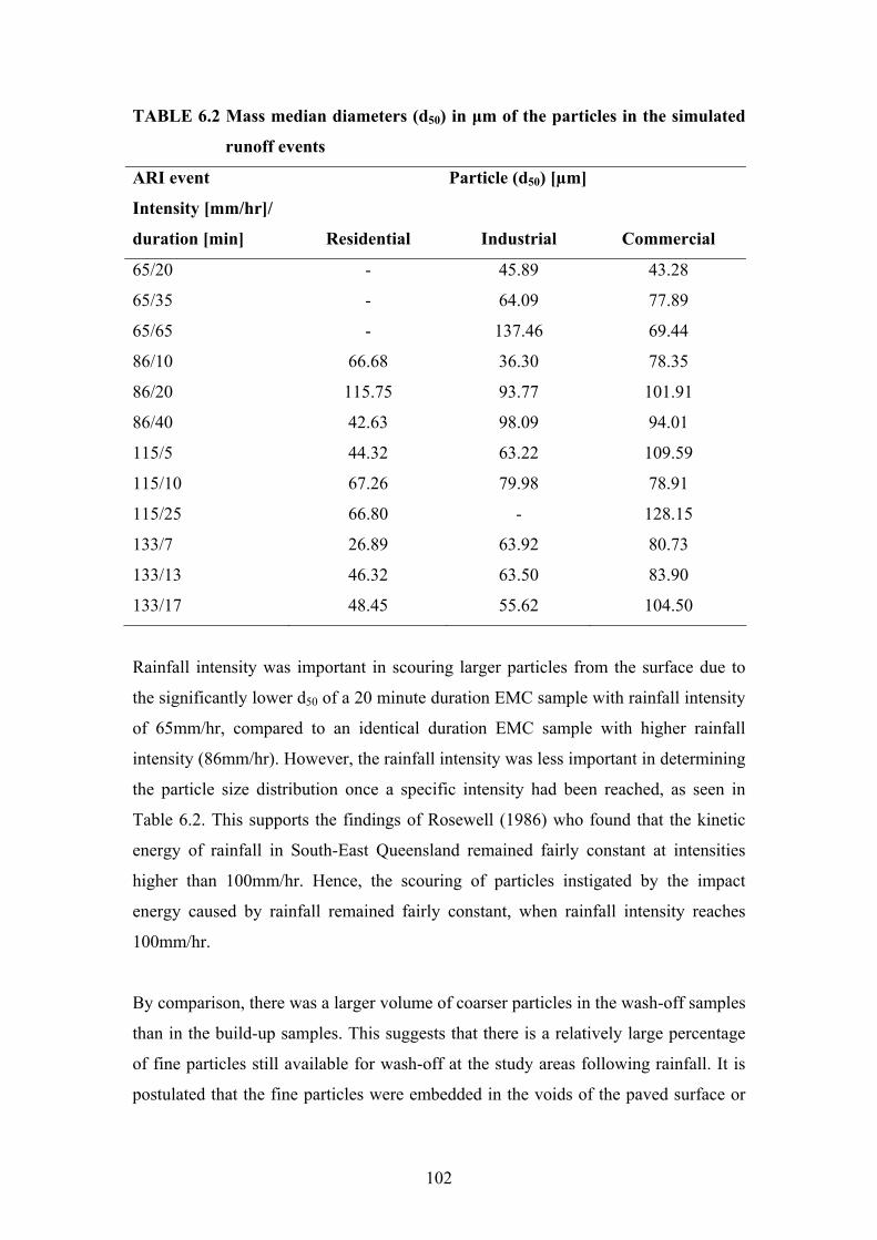
102
TABLE 6.2 Mass median diameters (d50) in μm of the particles in the simulated
runoff events
Particle (d50) [µm] ARI event
Intensity [mm/hr]/
duration [min] Residential Industrial Commercial
65/20 - 45.89 43.28
65/35 - 64.09 77.89
65/65 - 137.46 69.44
86/10 66.68 36.30 78.35
86/20 115.75 93.77 101.91
86/40 42.63 98.09 94.01
115/5 44.32 63.22 109.59
115/10 67.26 79.98 78.91
115/25 66.80 - 128.15
133/7 26.89 63.92 80.73
133/13 46.32 63.50 83.90
133/17 48.45 55.62 104.50
Rainfall intensity was important in scouring larger particles from the surface due to
the significantly lower d50 of a 20 minute duration EMC sample with rainfall intensity
of 65mm/hr, compared to an identical duration EMC sample with higher rainfall
intensity (86mm/hr). However, the rainfall intensity was less important in determining
the particle size distribution once a specific intensity had been reached, as seen in
Table 6.2. This supports the findings of Rosewell (1986) who found that the kinetic
energy of rainfall in South-East Queensland remained fairly constant at intensities
higher than 100mm/hr. Hence, the scouring of particles instigated by the impact
energy caused by rainfall remained fairly constant, when rainfall intensity reaches
100mm/hr.
By comparison, there was a larger volume of coarser particles in the wash-off samples
than in the build-up samples. This suggests that there is a relatively large percentage
of fine particles still available for wash-off at the study areas following rainfall. It is
postulated that the fine particles were embedded in the voids of the paved surface or

103
were re-deposited during the wash-off event at a point further downstream. Hence, the
wash-off of particles at the study sites was transport-limited instead of source-limited.
Thus, a relatively large pollutant load was available for wash-off independent of
antecedent dry period.
6.3.1 Partitioning of build-up and wash-off samples
The particle size distribution analysis revealed that the largest volume of particles in
the build-up samples were below 150µm, independent of land use characteristics.
More than 50% of the particles by volume were below 150µm in the wash-off
samples as shown in Table 6.2, independent of land use and rainfall characteristics.
Hence, it was decided to partition the build-up and wash-off samples for chemical
analysis based on these findings. This approach was supported by the findings of
Warren et al. (2003), who suggested that measuring ‘whole water’ (unfiltered)
concentrations of pollutants does not give an accurate indication of the processes
underlying the distribution of these pollutants. Furthermore, to effectively implement
stormwater management practices, knowledge of the distribution of pollutants in
different fractions are fundamental (Smith et al. 2000). Consequently, the dispersed
build-up and wash-off samples were separated into five particle size ranges by wet
sieving as described in Section 5.2.3. The five particle size ranges chosen were:
• Particles passing a 0.45µm filter (<0.45µm);
• Particles passing a 75µm sieve but not a 0.45µm filter (0.45-75µm);
• Particles passing a 150µm sieve but not a 75µm sieve (76-150µm);
• Particles passing a 300µm sieve but not a 150µm sieve (151-300µm); and
• Particles retained on a 300µm sieve (>300µm).
6.4 Chemical parameters
6.4.1 pH and EC
The Australian Laboratory Handbook of Soil and Water Chemical Methods (Rayment
and Higginson 1992) has specified methods for the measurement of pH and EC in soil
sediment (method 4A1 and 3A1 respectively). However, the methods described are
based on a 1:5 soil/water suspension and to get accurate results, a dry weight of 10g is
recommended. Therefore, pH and EC could not be measured accurately in the specific

104
particle sizes. Hence, pH and EC were only measured of the total build-up and wash-
off samples.
TABLE 6.3 pH and EC concentrations of the build-up sample at each site
Research site pH EC [μS/cm]
Residential 6.20 21.82
Industrial 6.43 25.10
Commercial 6.23 82.10
As can be seen in Table 6.3, the pH of the build-up samples showed no significant
change between the study sites. This is attributed to the prevalent soil conditions in
the study areas, which were of similar characteristics. This is supported by the small
difference in EC between the residential and industrial site as shown in Table 6.3.
However, the build-up sample from the commercial site had a significantly higher EC
than the other sites. This can be attributed to a number of reasons. Firstly, leakage and
spills of various fluids from parked vehicles will most likely have contributed to a
higher EC. In addition to this, the car park is surrounded by vegetation that it was
postulated, would be treated with fertiliser. Factors such as ocean salt transported by
vehicles and spills from various activities at the shopping centre could also have
contributed to the elevated EC. However, the largest contribution of salts was most
likely from the Nerang River, which flows just behind the shopping centre. The river
is affected by tidal flow at this location. Hence, soils around the river potentially
would have a higher EC than soils at the residential and industrial sites.
Similar to the build-up samples, the pH was relatively constant during the wash-off
events, independent of rainfall or land use characteristics, as shown in Table 6.4. This
is supported by the mean and standard deviation of the values measured in the wash-
off samples. For pH and EC measurements of individual samples from the residential,
industrial and commercial sites, refer to Tables B1-B3 Appendix B respectively.
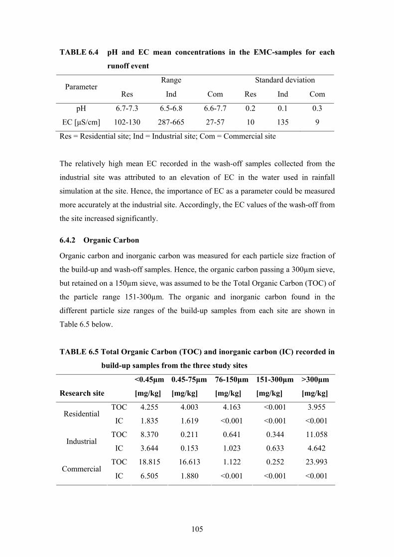
105
TABLE 6.4 pH and EC mean concentrations in the EMC-samples for each
runoff event
Range Standard deviation Parameter
Res Ind Com Res Ind Com
pH 6.7-7.3 6.5-6.8 6.6-7.7 0.2 0.1 0.3
EC [μS/cm] 102-130 287-665 27-57 10 135 9
Res = Residential site; Ind = Industrial site; Com = Commercial site
The relatively high mean EC recorded in the wash-off samples collected from the
industrial site was attributed to an elevation of EC in the water used in rainfall
simulation at the site. Hence, the importance of EC as a parameter could be measured
more accurately at the industrial site. Accordingly, the EC values of the wash-off from
the site increased significantly.
6.4.2 Organic Carbon
Organic carbon and inorganic carbon was measured for each particle size fraction of
the build-up and wash-off samples. Hence, the organic carbon passing a 300µm sieve,
but retained on a 150µm sieve, was assumed to be the Total Organic Carbon (TOC) of
the particle range 151-300µm. The organic and inorganic carbon found in the
different particle size ranges of the build-up samples from each site are shown in
Table 6.5 below.
TABLE 6.5 Total Organic Carbon (TOC) and inorganic carbon (IC) recorded in
build-up samples from the three study sites
Research site
<0.45μm
[mg/kg]
0.45-75μm
[mg/kg]
76-150μm
[mg/kg]
151-300μm
[mg/kg]
>300μm
[mg/kg]
TOC 4.255 4.003 4.163 <0.001 3.955 Residential
IC 1.835 1.619 <0.001 <0.001 <0.001
TOC 8.370 0.211 0.641 0.344 11.058 Industrial
IC 3.644 0.153 1.023 0.633 4.642
TOC 18.815 16.613 1.122 0.252 23.993 Commercial
IC 6.505 1.880 <0.001 <0.001 <0.001

106
TOC was always high in the largest particle size range (>300µm) independent of the
site. This could be attributed to the presence of twig and leaf fragments at all the sites.
At the commercial site there would also be a significant amount of organic carbon in
this particle size range originating from vehicle exhaust, so called soot particles
(Warren et al. 2003). However, a significant amount of TOC is distributed in particles
below 75µm. Sartor and Boyd (1972) found a similar distribution and hypothesised
that this could be due to the low structural strength of organic matter and that they can
be easily ground into fine particles. Another possible reason for a higher TOC in fine
particles could have been the relatively larger surface area of the particles. Hence,
non-particulate organic matter could adhere to the surface of fine particles as noted by
Warren et al. (2003). This in turn could have implications with respect to the transport
of heavy metals and PAHs to receiving waters in the region, as TOC has been found
to attract hydrophobic pollutants (Roger et al. 1998).
The inorganic carbon content of the build-up samples was very low and only detected
in particles below 75µm, except at the industrial site where IC was frequently detected
in the different particle size ranges. Whilst the presence of IC at the residential site
was postulated to be due to sand and dust-type materials, the presence of IC at the
industrial site was attributed to minerals originating from industrial activities. These
minerals could contain irreversibly trapped metals (Charlesworth and Lees 1999).
Consequently, mineral-like particles could transport a significant amount of metals to
receiving waters if incorporated into runoff. TOC was found primarily in dissolved
form (<0.45µm) in the wash-off samples independent of land use characteristics as
can be seen in Table 6.6, where mean TOC concentrations for each particle size at the
three sites are reported. This is most likely due to the presence of colloidal organic
matter at the sites.
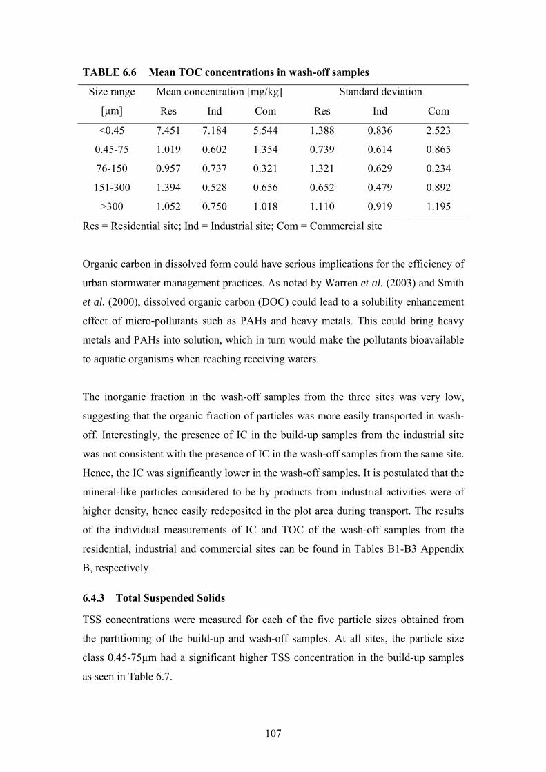
107
TABLE 6.6 Mean TOC concentrations in wash-off samples
Mean concentration [mg/kg] Standard deviation Size range
[μm] Res Ind Com Res Ind Com
<0.45 7.451 7.184 5.544 1.388 0.836 2.523
0.45-75 1.019 0.602 1.354 0.739 0.614 0.865
76-150 0.957 0.737 0.321 1.321 0.629 0.234
151-300 1.394 0.528 0.656 0.652 0.479 0.892
>300 1.052 0.750 1.018 1.110 0.919 1.195
Res = Residential site; Ind = Industrial site; Com = Commercial site
Organic carbon in dissolved form could have serious implications for the efficiency of
urban stormwater management practices. As noted by Warren et al. (2003) and Smith
et al. (2000), dissolved organic carbon (DOC) could lead to a solubility enhancement
effect of micro-pollutants such as PAHs and heavy metals. This could bring heavy
metals and PAHs into solution, which in turn would make the pollutants bioavailable
to aquatic organisms when reaching receiving waters.
The inorganic fraction in the wash-off samples from the three sites was very low,
suggesting that the organic fraction of particles was more easily transported in wash-
off. Interestingly, the presence of IC in the build-up samples from the industrial site
was not consistent with the presence of IC in the wash-off samples from the same site.
Hence, the IC was significantly lower in the wash-off samples. It is postulated that the
mineral-like particles considered to be by products from industrial activities were of
higher density, hence easily redeposited in the plot area during transport. The results
of the individual measurements of IC and TOC of the wash-off samples from the
residential, industrial and commercial sites can be found in Tables B1-B3 Appendix
B, respectively.
6.4.3 Total Suspended Solids
TSS concentrations were measured for each of the five particle sizes obtained from
the partitioning of the build-up and wash-off samples. At all sites, the particle size
class 0.45-75µm had a significant higher TSS concentration in the build-up samples
as seen in Table 6.7.
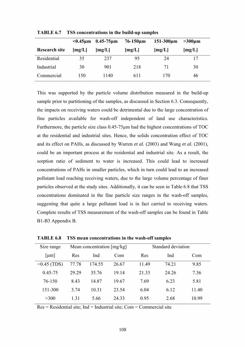
108
TABLE 6.7 TSS concentrations in the build-up samples
Research site
<0.45μm
[mg/L]
0.45-75μm
[mg/L]
76-150μm
[mg/L]
151-300μm
[mg/L]
>300μm
[mg/L]
Residential 35 237 95 24 17
Industrial 30 901 218 71 30
Commercial 150 1140 611 170 46
This was supported by the particle volume distribution measured in the build-up
sample prior to partitioning of the samples, as discussed in Section 6.3. Consequently,
the impacts on receiving waters could be detrimental due to the large concentration of
fine particles available for wash-off independent of land use characteristics.
Furthermore, the particle size class 0.45-75µm had the highest concentrations of TOC
at the residential and industrial sites. Hence, the solids concentration effect of TOC
and its effect on PAHs, as discussed by Warren et al. (2003) and Wang et al. (2001),
could be an important process at the residential and industrial site. As a result, the
sorption ratio of sediment to water is increased. This could lead to increased
concentrations of PAHs in smaller particles, which in turn could lead to an increased
pollutant load reaching receiving waters, due to the large volume percentage of finer
particles observed at the study sites. Additionally, it can be seen in Table 6.8 that TSS
concentrations dominated in the fine particle size ranges in the wash-off samples,
suggesting that quite a large pollutant load is in fact carried to receiving waters.
Complete results of TSS measurement of the wash-off samples can be found in Table
B1-B3 Appendix B.
TABLE 6.8 TSS mean concentrations in the wash-off samples
Mean concentration [mg/kg] Standard deviation Size range
[μm] Res Ind Com Res Ind Com
<0.45 (TDS) 77.78 174.55 26.67 11.49 74.21 9.85
0.45-75 29.29 35.76 19.14 21.33 24.26 7.36
76-150 8.43 14.87 19.67 7.69 6.23 5.81
151-300 3.74 10.31 23.54 6.04 6.12 11.40
>300 1.31 5.66 24.33 0.95 2.68 10.99
Res = Residential site; Ind = Industrial site; Com = Commercial site

109
However, it can also be seen that a higher concentration of solids was carried by the
dissolved fraction in wash-off, as indicated by the relatively high TDS concentrations
(particles <0.45µm) found in the wash-off samples compared to the build-up samples.
This is most likely due to colloidal organic particles transported in the dissolved
fraction, suggested by the amount of dissolved organic carbon (DOC) found at the
sites. This supports the finding by Sartor and Boyd (1972) who noted the low
structural strength of organic matter, which is easily ground into finer particles.
The TSS concentrations of the different particle size classes of the wash-off samples
collected at the commercial site showed a slightly different distribution to the other
study areas. The TSS concentrations were fairly evenly distributed between the
particle size classes, which was attributed to the coarse texture depth recorded at the
parking lot. Hence, fine particulates could be trapped in the voids of the paved surface
and not incorporated into runoff. However, frequent traffic at the site and street
sweeping has the potential to release a significant amount of these particles from the
voids, which could lead to higher concentrations of fine particles available for wash-
off at the next event. Furthermore, at the time of sampling at the commercial site,
there was a very light natural rainfall event occurring. Consequently, fine particles
could have been transported by the runoff generated from this natural rainfall event,
leaving coarser particles behind that were incorporated into the wash-off from the
simulated rainfall.
6.4.4 Heavy metals
Metal concentrations were measured in each particle size class of the build-up and
wash-off samples. The highest metal concentrations were consistently found in the
0.45-75µm of the build-up samples, followed by the 76-150µm size range as shown in
Table 6.9, which coincided with highest concentrations of TSS. As a result, the
highest heavy metal load at the three study sites was consistently found in fine
particles, which further strengthens the importance of removing fine particles in urban
stormwater quality management.

110
TABLE 6.9 Heavy metal concentrations in each particle size at the three sites
Metal
<0.45μm
[mg/kg]
0.45-75μm
[mg/kg]
76-150μm
[mg/kg]
151-300μm
[mg/kg]
>300μm
[mg/kg]
Fe 0.007 13.997 12.799 3.480 1.480
Zn 0.390 1.800 0.720 0.288 0.136
Al 0.008 8.800 8.800 2.640 1.240
Pb <0.001 0.044 0.034 0.010 0.005
Cu 0.082 0.560 0.480 0.680 0.344
Cd <0.001 0.002 0.002 0.001 0.001
Cr <0.001 0.018 0.014 0.008 0.006
Res
iden
tial
Mn 0.008 0.228 0.200 0.056 0.028
Fe <0.005 43.960 2.160 0.616 1.360
Zn 0.180 2.318 0.112 0.039 0.080
Al 0.009 13.588 0.632 0.240 0.464
Pb 0.002 0.959 0.035 0.010 0.019
Cu 0.007 0.959 0.037 0.040 0.043
Cd <0.001 <0.001 <0.001 <0.001 <0.001
Cr <0.001 0.063 0.003 0.002 0.013
Indu
stria
l
Mn 0.022 0.512 0.022 0.008 0.014
Fe 0.960 16.781 9.594 4.719 3.840
Zn 0.830 0.424 0.296 0.112 0.060
Al 0.069 5.514 3.518 1.760 1.280
Pb 0.014 0.344 0.192 0.088 0.051
Cu 0.120 0.264 0.240 0.528 0.224
Cd 0.003 0.002 0.008 <0.001 <0.001
Cr <0.001 0.026 0.015 0.008 0.006
Com
mer
cial
Mn 0.270 0.224 0.160 0.072 0.057
The least detected heavy metals in the build-up samples were Cd followed by Cr.
These metals have been linked with brakes and tyres of vehicles (Sansalone and
Buchberger 1997). Hence, the larger traffic volume observed at the residential and
commercial site, compared to the infrequent high vehicle traffic observed at the
industrial site, is postulated to have influenced the presence of these metals in the

111
environment. However, this is a typical example where pattern recognition using
multivariate analysis was useful in analysing sources and processes in relation to the
pollutants. PCA helped identifying the sources of these metals at the sites, which is
further discussed in Chapter 7. The most frequently detected metals at each site were
Al and Fe. These metals have been attributed to common minerals present in soils
(Pierson and Brachaczek 1983).
The highest concentration of Zn in the build-up samples occurred in colloidal size
particles (<0.45µm). It is postulated that the presence of Zn is affected by the DOC
available in this particle size class. Similar correlations between Zn and organic
carbon content have been found by several researchers (Ellis et al. 1987; Morrison et
al. 1984), which suggests that metal-organic complexation was occurring in the build-
up samples. Consequently, the increased bioavailability of Zn due to metal-organic
complexation highlights the importance of understanding fundamental processes in
urban stormwater. Furthermore, organic carbon was also found in relatively high
concentrations in the largest particle size class of the build-up samples analysed in the
three sites. In spite of this, the TOC content had a lesser effect on the distribution of
heavy metals in this size class. This could be due to the lesser sorption capacity of
larger particles (Dong et al. 1984; Ujevic et al. 2000). Another reason could be the
difference in the type and nature of sediment, which can be attributed to the source of
the organic matter present (Warren et al. 2003). This in turn could influence the
interaction between heavy metals and particles.
Similar to the build-up samples, the highest metal concentrations were found in the
particle size class 0.45-75µm of the wash-off samples independent of land use and
rainfall characteristics. It was found that the rainfall intensity had little or no effect on
the distribution of heavy metals. However, the metal concentrations in the EMC
samples generally decreased with duration, suggesting that a dilution effect was
occurring. Table 6.10 shows the concentration range of each metal in the wash-off
samples from each site independent of particle size class. Complete results of the
metal analysis can be found in the raw data tables for each site, Table B1-B3
Appendix B (Residential, Industrial and Commercial respectively).

112
TABLE 6.10 Metal concentration ranges observed in particulate and dissolved
fractions of wash-off samples from each site [ppm]
Range [ppm] Standard deviation
Res Ind Com Res Ind Com
Zn <0.001-3.6 <0.001-0.5 <0.001-0.7 0.7 0.1 0.2
Cu <0.001-0.4 <0.001-0.04 <0.001-0.1 0.08 0.007 0.03
Pb <0.001-0.02 <0.001-0.03 <0.001-0.01 0.002 0.005 0.002
Al <0.001-0.6 <0.001-0.4 <0.001-0.3 0.2 0.09 0.05
Fe <0.001-0.7 <0.001-0.9 <0.001-0.7 0.2 0.2 0.1
Cd <0.001-0.3 <0.001-0.001 <0.001 0.05 0.0002 <0.001
Cr <0.001-0.007 <0.001-0.02 <0.001-0.003 0.002 0.003 0.001
Mn <0.001-0.01 <0.001-0.02 <0.001-0.01 0.003 0.004 0.003
Res = Residential site; Ind = Industrial site; Com = Commercial site
Interestingly, the highest concentration of a number of the metals analysed were
observed at the residential site, primarily Cu and Zn. This was attributed to the fact
that most of the particles available on the paved surface were incorporated into wash-
off at the residential site due to the fine texture of the surface. Hence, the coarser
street texture recorded at the industrial and commercial site restrained metals attached
to particles from being incorporated into wash-off. Therefore, it could be more
important to implement efficient urban stormwater management measures in a
residential area. However, this would depend largely on the street surface texture.
Additionally, frequent rainfall events with a lower intensity could significantly
influence the amount of particles scoured from the surface due to lower impact
energy. This issue was not investigated in this research.
The industrial site had the highest concentrations of Pb, Fe, Mn and Cr, which were
postulated to be attributed to the metal-based industries at the site. This is further
discussed in Chapter 7.
6.4.5 Polycyclic Aromatic Hydrocarbons (PAHs)
The initial results of the analysis undertaken indicated that it was only necessary to
investigate the PAH concentrations in four different particle size classes. It was found

113
that PAH concentrations in particles larger than 300µm were low compared to the
remaining particle sizes. Less than 15% of the individual PAH concentrations were
found in particles above 300µm. Consequently, it was decided that the particle size
classes 151-300µm and >300µm could be combined without losing vital information.
The particle size classes that were analysed for PAHs therefore were:
• <0.45µm;
• 0.45-75µm;
• 76-150µm; and
• >150µm.
Similar to the heavy metal concentrations, PAH concentrations dominated in particle
sizes below 150µm, independent of study site as shown in Table 6.11, which reports
PAH concentrations in each particle size class of the build-up samples. This is
attributed to the higher adsorption affinity of finer particles due to their relatively
larger surface area and electrostatic charge (Andral et al.1999; Roger et al. 1998).

114
TABLE 6.11 PAH concentrations [mg/kg] in the build-up samples from each site
Particle size range [μm] NAP ACY ACE FLU PHE ANT FLA PYR BaA CHR BbF* BaP IND DbA BgP
<0.45 0.08 0.02 <0.01 <0.01 <0.01 <0.01 0.01 <0.01 <0.01 <0.01 <0.01 <0.01 <0.01 <0.01 <0.01
0.45-75 1.16 0.12 0.17 0.11 0.21 0.13 0.28 0.38 0.27 <0.01 0.15 0.22 <0.01 <0.01 <0.01
76-150 1.26 0.16 0.11 0.14 0.21 0.15 0.25 0.30 0.30 <0.01 <0.01 0.24 <0.01 <0.01 <0.01
Res
iden
tial
>150 0.92 0.06 0.03 <0.01 <0.01 0.03 0.05 0.54 0.21 <0.01 <0.01 0.15 <0.01 <0.01 <0.01
<0.45 0.06 0.02 0.02 <0.01 <0.01 <0.01 0.02 <0.01 <0.01 <0.01 <0.01 <0.01 <0.01 <0.01 <0.01
0.45-75 2.50 0.28 0.34 0.17 0.15 0.11 0.27 0.32 0.17 0.31 0.14 0.18 0.05 <0.01 0.03
76-150 2.15 0.35 0.40 0.12 0.13 0.10 0.10 0.15 0.16 0.31 0.11 0.16 <0.01 <0.01 0.02
Indu
stria
l
>150 1.48 0.28 0.10 0.06 0.08 <0.01 0.14 0.17 0.13 0.17 0.11 0.27 <0.01 <0.01 <0.01
<0.45 0.89 0.09 0.05 0.02 0.02 <0.01 0.03 0.01 0.03 <0.01 <0.01 0.12 <0.01 <0.01 <0.01
0.45-75 15.32 1.77 1.45 0.86 1.85 0.21 0.87 0.87 0.76 0.56 0.56 0.90 0.31 0.17 0.06
76-150 4.88 1.24 0.76 0.65 1.53 0.19 0.68 0.56 0.65 0.65 0.37 0.66 0.21 0.05 0.05
Com
mer
cial
>150 2.53 0.65 0.26 0.15 0.17 0.05 0.53 0.45 0.13 0.08 0.21 0.15 <0.01 0.01 <0.01
* Benzo[b]flouranthene (BbF) and Benzo[k]flouranthene (BkF) were measured as one parameter

115
PAH concentrations were always low in colloidal size particles in the build-up
samples. This is attributed to the low solubility of PAHs, which decreases with
increasing molecular weight (Manoli and Samara 1999). It was no surprise that the
most detected PAH in colloidal particles was NAP, which is a two-ring PAH.
PAHs were detected frequently in the build-up samples as shown in Table 6.11.
However, higher molecular weight PAHs such as IND were not detected at the
residential and industrial site. The commercial site had low concentrations of high
molecular weight, which could be attributed to the traffic volume at the site. Bae et
al. (2002) found IND to be a typical by-product of petrol engines, which supports the
higher presence of this PAH at the commercial site. This is further assessed using
multivariate methods in the recognition of sources and processes in Chapter 7.
Among the 16 individual PAHs analysed, the two-ring PAH, NAP was the most
frequently detected element in wash-off samples independent of particle size class
followed by the three-ring PAH, ACY, as shown in Table 6.12. Mean concentrations
of PAHs in each particle size range can be found in Tables B4-B6 Appendix B, for the
residential, industrial and commercial sites respectively. The commercial site had the
highest mean PAH concentrations of the three study sites including the highly
carcinogenic BaP. The frequent detection of high molecular-weight PAHs in wash-off
from the commercial site can be attributed to the higher availability of PAHs observed
in the build-up samples. Similar to the heavy metal concentrations observed at the
residential site, the PAH concentrations in wash-off from the site was frequently
higher than in wash-off from the industrial site. This was attributed to the finer texture
of the paved surface observed at the residential site. However, it could also be
attributed to higher source strength of PAHs in the residential area compared to the
industrial area. It is postulated that the lifestyle in the residential area could generate a
significant amount of PAHs through frequent car washing or application of gardening
chemicals. Furthermore, PAHs at the residential site were found above their aqueous
solubility, which could be due to petrogenic sources such as oil spills and petrol spills.
Hence, oil and grease emulsions could have been formed. This is supported by Smith
et al. (2000) who noted PAH concentrations above aqueous solubility to be due to oil
and grease emulsions passing a 0.45μm filter. Similar to this, PAHs were found above
their aqueous concentrations in wash-off samples from the commercial site, which

116
could be attributed to oil and petrol leakage from parked cars as noted by Readman et
al. (1987). In addition to this, the aqueous concentrations of PAHs observed could
also be due to the presence of organic colloidal particles as indicated by the DOC
reported in the wash-off samples. Consequently, the presence of DOC in the wash-off
samples could enhance the solubility of PAHs, which in turn could increase their
bioavailability (Warren et al. 2003; Smith et al. 2000).
TABLE 6.12 Detection frequencies (%), mean concentration (mg/kg) and
standard deviation of 16 PAHs in wash-off samples from the
residential, industrial and commercial sites
Residential Industrial Commercial
PAH DF Mean SD DF Mean SD DF Mean SD
NAP 97 0.80 0.43 100 1.11 0.81 98 2.01 2.21
ACY 53 0.11 0.07 82 0.14 0.10 85 0.33 0.26
ACE 22 0.06 0.03 77 0.17 0.13 77 0.12 0.12
FLU 14 0.09 0.04 57 0.05 0.04 67 0.16 0.18
PHE 22 0.14 0.07 57 0.08 0.06 60 0.30 0.34
ANT 31 0.12 0.06 43 0.06 0.03 54 0.07 0.05
FLA 44 0.18 0.10 82 0.09 0.07 79 0.19 0.19
PYR 44 0.14 0.09 61 0.12 0.08 69 0.18 0.14
BaA 31 0.13 0.07 70 0.08 0.05 71 0.20 0.16
CHR 6 0.13 0.03 52 0.14 0.09 60 0.13 0.11
BbF* 11 0.11 0.04 52 0.04 0.03 58 0.23 0.18
BaP 42 0.13 0.08 75 0.08 0.05 85 0.14 0.11
IND 0 <0.01 <0.01 20 0.02 0.01 31 0.08 0.05
DbA 0 <0.01 <0.01 0 <0.01 <0.01 19 0.04 0.02
BgP 0 <0.01 <0.01 34 0.02 0.01 33 0.04 0.02
DF = Detection Frequency; SD = Standard deviation from mean;
* Benzo[b]flouranthene (BbF) and Benzo[k]flouranthene (BkF) were measured as one
parameter
However, the vast majority of PAHs were associated with the particulate phase of
runoff independent of land use and rainfall characteristics, as can be seen in Table
117
6.12. This can be attributed to the primary source being pyrogenic sources such as the
incomplete combustion of fossil fuels. Potential sources of the PAHs present at the
study areas and identification of PAH distribution processes were assessed using PCA
as described in Chapter 7.
6.5 Summary
Prior to chemical analysis, particle size distribution of the build-up and wash-off
samples collected at each site were investigated. The results indicate that as much as
90% of the volume of particles in the build-up and wash-off samples was smaller than
150µm. Consequently, in order to develop an in-depth understanding of the
distribution processes occurring in build-up and wash-off from the three study sites,
the samples were fractionated into different particle size classes. Samples investigated
for heavy metal concentrations were partitioned into five particle size classes, while
samples investigated for PAH concentrations were partitioned into four different
particle size classes, due to initial analysis undertaken indicating that the majority of
PAHs were attached to particles less than 150μm.
Heavy metal and PAH concentrations were highest in the 0.45-75µm particle size
class of the build-up and wash-off samples, independent of land use and rainfall
characteristics. This coincided with the highest TSS concentrations reported.
However, individual metals and PAHs were affected by the DOC present, which
increased the concentration of PAHs and metals in the dissolved phase of runoff.
PAHs were often found in concentrations above their aqueous solubility, which was
attributed to source characteristics such as oil and petrol spills, and the presence of
colloidal organic particles introducing a solubility enhancement effect on PAHs. The
transport of PAHs and heavy metals in the dissolved phase of wash-off could have a
significant effect on aquatic organisms in receiving waters, due to their increased
bioavailability. Furthermore, a significant amount of PAHs and heavy metals are
transported by fine particles in wash-off, which could have implications on urban
stormwater measures such as street sweeping and detention basins due to their
inability in removing finer particles.
More importantly, the mean concentrations and standard deviations reported in this
chapter highlighted the need for multivariate methods in analysing complex data

118
matrices. Complimentary information such as source recognition and pattern
distribution could be identified using common chemometrics methods such as
Principal Component Analysis (PCA), which reduces the number of components
involved to a set of principal components. Furthermore, the relationships between
parameters that can be identified can also be validated using a multivariate
chemometrics approach such as Partial Least Square (PLS) regression. This in turn
could lead to an increased transferability of fundamental concepts relating to urban
water quality which is an essential problem in urban stormwater and its management.
Consequently, the advantages with a multivariate approach to urban water quality
studies can be many and are highlighted in Chapter 7 and 8.

119
Chapter 7 Pattern and Process Recognition using PCA
7.1 Introduction
Multivariate analytical methods were found to be preferable to understand the
processes governing the build-up and wash-off of PAH and heavy metals in urban
areas. The relative importance of the variables involved in distribution processes of
these pollutants was difficult to quantify using univariate analysis. Hence,
multivariate chemometrics approaches to urban water quality studies were necessary
to fully understand relationships between parameters and the processes underlying the
distribution of micro-pollutants.
Univariate analysis can only be used to compare two parameters against each other.
However, the heavy metal concentrations were most likely affected by a number of
parameters and the relative importance of each parameter was difficult to investigate
using univariate methods. Similarly, PAH concentrations could be influenced by
different physico-chemical parameters as well as the source characteristics depending
on the PAH (Kucklick et al. 1997). Therefore, multivariate analysis was preferred,
since a large data volume can be processed in order to explore and understand
relationships between variables and objects (Kokot et al. 1998).
This chapter will focus on the results obtained from the Principal Component
Analysis (PCA). PCA was employed on the data set to identify correlations between
parameters and the possible sources of pollutants at the respective study sites. PCA
was also employed to identify processes that were important in the distribution of
PAHs and heavy metals in build-up and wash-off at the three sites.
7.2 Applications of Principal Component Analysis
The most common pattern recognition method used in multivariate analysis is
Principal Component Analysis (PCA). PCA has been successfully applied to a range
of different data sets in previous research, such as process identification in river water
quality data (Petersen et al. 2001) and to identify parameter relationships of lake-
polluted sediments (De Bartolomeo et al. 2004). In spite of this, as noted by Kokot et
al. (1998), though multivariate analysis can provide complementary information and

120
often produce solutions unobtainable by conventional data interpretation, the
experimental possibilities of chemometrics applications are quite poorly understood.
This is primarily attributed to the difficulty with multidimensional thinking and the
different approaches used in multivariate analysis compared to conventional statistical
approaches. However, multivariate analysis can contribute to significant
improvements in the interpretation of urban water quality data, if applied correctly.
This commonly entails significant pre-treatment of data prior to chemometrics
methods being applied. Nevertheless, chemometrics cannot rectify poor sampling or
analytical laboratory techniques.
PCA is one of the most important techniques employed in chemometrics (Kokot et al.
1998). The central idea behind PCA is to reduce a set of data consisting of a large
number of variables to a much smaller number of orthogonal components that retain
as much as possible of the information available in the original data (Massart et al.
1990). The new variables are linear and called principal components and are estimated
from the eigenvectors of the covariance matrix of the original variables. The PCA
method is described mathematically in Appendix C page 279. The number of
principal components to be used is then determined using the scree plot method
described by Cattell (1966), or by setting the number of principal components to the
number of eigenvalues, generated by PCA, greater than 1 (Kaiser 1960). The scree
plot method, which plots the eigenvalue extracted for each principal component, was
implemented in this research. It is usually shaped like a cliff with a scree slope at the
bottom, an initially sharp descending gradient, as the most important factors are
extracted, which is followed by a gentler gradient corresponding to minor factors.
Finally, the graph flattens out completely as the point of diminishing returns is
reached. Further factors contribute little to the analysis, and may be considered to be
artifacts. PCA was especially useful in this research due to the ability to substantially
reduce the dimensionality of the original data which contained a number of physico-
chemical variables as well as eight metal elements and 16 PAHs.
To apply PCA to a data set, the original data must be arranged into a matrix with
selected variables defining the columns and the rows referred to as sample
measurements or objects. PCA can be applied to this ‘raw’ data set, or it can be pre-
treated to reduce data heterogeneity and reduce irrelevant sources of variation or

121
noise. Normal pre-treatment options include log-transformation of the original data
and column standardisation (Kokot et al. 1998; Kettaneh et al. 2005). Column
standardisation of the data means that each cell in a given column is divided by the
standard deviation of that particular column. Hence, each variable is equally weighted
with a standard deviation of one.
The application of PCA to a data matrix generates a loading for each variable and a
score for each object (build-up and wash-off samples in the case of this research) on
the principal components. Consequently, the data can be presented diagrammatically
by plotting the scores of each object on selected principal components (referred to as a
scores plot), or the loading or importance of each variable on the selected principal
components (referred to as a loadings plot). The relationships between objects and
variables can also be displayed using a biplot, which is a combination of the scores
and loadings plots. A vector drawn from the origin to a set of loadings coordinates on
the biplot represents the size of the loadings of the variables on the respective
principal components. Additionally, it indicates the likely objects (samples) with
which the specific variable is particularly associated.
The software used in this research to undertake PCA was MatLab. The PCA
algorithms used in the research were adopted from Kramer (1993) and are
summarised in Appendix C page 280.
7.3 Pre-treatment of data
Prior to analysis, the concentration data reported for each variable in the build-up and
wash-off samples (refer to Chapter 6) was log transformed to remove large variations
without interfering with the variance of the data set. As an example, TSS could vary
from 10-1000mg/L, while TOC concentration could vary between 1-8mg/L in the
build-up samples. Hence, log transforming the data removed the skewness of the data.
Similarly, the data was mean-centred in order to compensate for different units of
measurement or scale. All data below detection limit of the analytical instrument used
for determining the parameters was set to half the detection limit value in the PCA
(Guo et al. 2004). Parameters not detected were excluded from the data set when
necessary. For example, three PAHs (IND, DbA and BgP) were not detected in any
fraction of the build-up and wash-off samples from the residential site. These PAHs

122
could not be included in the analysis of the specific land use and were therefore
excluded from the residential data set prior to PCA application.
PCA was undertaken on each individual particle size class (wash-off samples only) as
well as bulk samples (build-up samples only) in order to determine trends and patterns
that might be dependent or independent of particle size. Consequently, it was
postulated that processes governing the partition of heavy metals and PAHs between a
dissolved and particulate fraction in wash-off samples could be different to
distribution processes of the pollutants in different particle size classes. The
parameters included in the PCA were given an abbreviation as listed in Table 7.1.
Particle volume percentage (PVP) of the build-up and wash-off samples was
considered an important parameter due to the increased load that can be attributed to
any pollutant associated with PVP. As Pitt (1979) noted, the shock pollutant load that
can result from a stormwater runoff event can have a detrimental impact on the
quality of receiving waters. Similarly, increases in total PAH concentrations have
been found to be mirrored by an increase in TSS concentration (Hoffman et al. 1984).
However, Hoffman et al. (1984) found individual PAHs to differ from this behaviour,
which the authors attributed primarily to difference in solubility and particle size
distribution. Hence, it is important to investigate PVP as well as TSS of urban runoff.
This could lead to significant improvements in stormwater management such as the
knowledge of which pollutants and particle sizes to target to efficiently reduce
impacts on receiving waters. Organic carbon content (TOC, DOC dependent of the
fraction) was also included in the analysis due to its ability to enhance the solubility of
PAHs and increase solid binding affinity when in particulate form (Warren et al.
2003). The influence of organic carbon on stormwater has been extensively discussed
in Chapter 2.
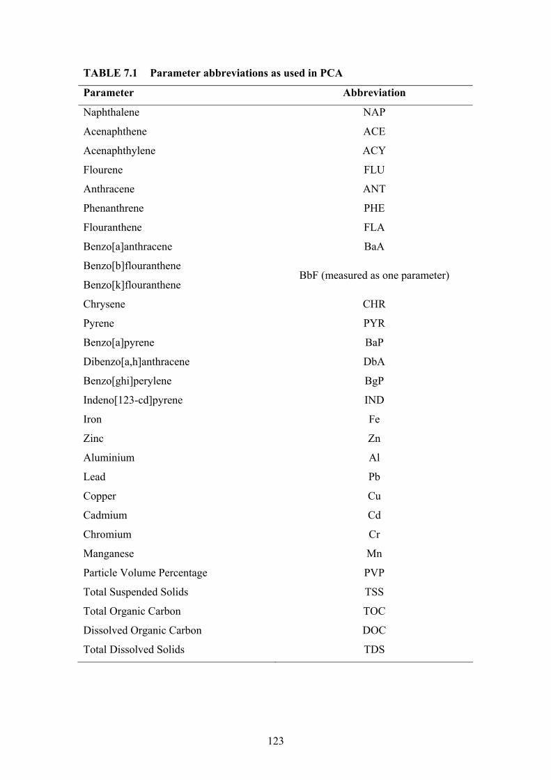
123
TABLE 7.1 Parameter abbreviations as used in PCA
Parameter Abbreviation
Naphthalene NAP
Acenaphthene ACE
Acenaphthylene ACY
Flourene FLU
Anthracene ANT
Phenanthrene PHE
Flouranthene FLA
Benzo[a]anthracene BaA
Benzo[b]flouranthene
Benzo[k]flouranthene BbF (measured as one parameter)
Chrysene CHR
Pyrene PYR
Benzo[a]pyrene BaP
Dibenzo[a,h]anthracene DbA
Benzo[ghi]perylene BgP
Indeno[123-cd]pyrene IND
Iron Fe
Zinc Zn
Aluminium Al
Lead Pb
Copper Cu
Cadmium Cd
Chromium Cr
Manganese Mn
Particle Volume Percentage PVP
Total Suspended Solids TSS
Total Organic Carbon TOC
Dissolved Organic Carbon DOC
Total Dissolved Solids TDS
124
7.4 Build-up samples
Only one build-up sample was collected at each site as it was considered adequate to
determine the characteristics of the pollutants available on the paved surface. This was
based on an implicit assumption that the pollutant build-up similar over the paved
surface. This was attributed to the small distance between the build-up and wash-off
plots used for the experiment. The spatial variation was considered minimal in such a
small area. As discussed in Chapter 6, the samples obtained were separated based on
the particle size distribution and pollutants investigated. The large variance observed
in the data set, together with the large number of variables investigated, made it
difficult to draw any conclusions from univariate analysis, even though only five
objects at each site were investigated. PCA was undertaken on build-up data from the
three study areas separately. Consequently, processes that were responsible for the
distribution of PAHs and heavy metals in accumulated particles on the street surfaces
could be identified and compared for each site. It was decided to undertake PCA on
the separate build-up samples due to pollutant concentrations being different at the
three sites, which could skew the PCA. Moreover, the detection of PAHs was very
site-specific in the build-up samples as shown in Chapter 6, which could further bias
the results from PCA.
7.4.1 Residential site
The scree plot method developed by Cattell (1966) was adopted to determine the
number of principal components to use in describing the PCA results of the residential
data. The number of principal components was determined as two by identifying the
position of the elbow or steep reduction in slope in the scree plot as shown in Figure
7.1. PC1 and PC2 contained 94.1% (81.4% and 12.7% respectively) of the total
variance in the build-up data at the residential site.

125
FIGURE 7.1 Scree plot for the determination of number of components to use in
exploring residential build-up data
The loading of each variable on PC1 and PC2 is shown by the loadings plot in Figure
7.2.
FIGURE 7.2 Loadings of each variable on PC1 and PC2 obtained from PCA on
residential build-up data
ELBOW
FLU, TSS, BbF, Zn, PHE
Cd, BaA, Cr, NAP, BaP, Al, Fe
Quadrant 1
Quadrant 2

126
Since variables in general agreement are orientated in the same direction in the
loadings plot (Kokot et al. 1998), it can be seen that a number of metals and PAHs
were inter-related. Furthermore, two quadrants of the loadings plot contained all the
metal and PAH data. These were:
• Quadrant 1 - Variables with a positive loading on both PC1 and PC2; and
• Quadrant 2 - Variables with positive loading on PC1 but negative loading on PC2.
The majority of PAHs were associated with Quadrant 2, while the majority of metals
are associated with Quadrant 1. However, most of the data variance was explained in
PC1 (81.4%). The positive loading of all heavy metals and PAHs on PC1 indicated
that a majority of PAHs and metals originated from a similar source. It is postulated
that the primary input of the metals and PAHs was traffic-related. Similar results
have been found by numerous researchers (Bomboi and Hernandez 1991; Harrison et
al. 2003; Manoli et al. 2000). The PAHs were separated by the loadings on PC2
depending on their molecular weight. As can be seen in Figure 7.2, PAHs with 3- and
4-rings were associated with Quadrant 1 and 4- or higher ring PAHs were associated
with Quadrant 1. This suggests that additional sources were responsible for some of
the PAHs present at the residential site. It is postulated that atmospheric deposition
and the lifestyle of the area could have been responsible for an appreciable amount of
PAHs being deposited on the road. This is supported by Bae et al. (2002) who
suggested that higher molecular weight PAHs were mainly associated with air-borne
particles. Nevertheless, atmospheric particulate bound PAHs are mostly deposited
regionally while PAHs in the gas phase (2- to 3-ring PAHs) can be transported longer
distances (Bucheli et al. 2004). Therefore, the PAHs associated with Quadrant 2 in
Figure 7.2 were most likely introduced by neighbouring industrial activities or
particles originating from vehicle exhaust in the area, while an appreciable amount of
the low molecular-weight NAP (Quadrant 1) could have been transported over a long
range.
Bomboi and Hernandez (1991) found the presence of PAHs at residential and
landscaped areas to be derived from gardening products and higher vascular plants,
especially NAP. Consequently, NAP could have originated from numerous sources,
127
both locally and long-range transported. However, the importance of PAHs in
Quadrant 1 in urban stormwater management is debatable. This is due to the
correlation between PAHs in Quadrant 2 and PVP and TSS. As a result, PAHs in
Quadrant 2 could potentially have a lower concentration than PAHs in Quadrant 1,
but carry a higher load of PAHs to receiving waters due to the affinity with TSS and
PVP. This finding is of significant importance in developing best management
practices for residential areas. Hence, removing the particle size range with the
highest TSS concentration and PVP percentage could significantly reduce the amount
of PAHs being incorporated into runoff. Additionally, PAHs and heavy metals in
Quadrant 2 were associated with particles between 0.45-150µm as can be seen by its
score in the scores plot in Figure C1 Appendix C. This suggests that current street
sweeping measures in the residential area could be inefficient in removing PAHs and
heavy metals from the paved surface due to limitations in street sweeping techniques,
as observed by previous researchers (Bender and Terstriep 1984; Sutherland et al.
1998).
Similar to the PAHs, the heavy metals were separated by the loadings on PC2 into
Quadrant 1 and Quadrant 2. The majority of the metals were associated with Quadrant
1 except Zn which was associated with Quadrant 2. It is postulated that an additional
source to traffic, such as the corrosion of galvanised roofs in the residential area is
responsible for this separation on PC2. Furthermore, it is postulated that an
appreciable amount of metals would originate from the local soils. This is
strengthened by the correlation between Al and Fe in Quadrant 1 in Figure 7.2.
Previous research has shown that soil dust can account for over 60% of the Al and Fe
load (Pierson and Brachaczek 1983), confirming that the deposition of eroded soil
particles is an important pollutant source at the residential site. Pb and Mn are
primarily traffic-related metals, which are shown by their low loading on PC2. Cu is
separated from the other metals in Quadrant 1 suggesting an additional source could
be contributing to the street deposited sediments. Ball et al. (1998) attributed the
presence of Cu in residential areas to by-products from garden refuse. In addition to
this, Makepeace et al. (1995) suggested that Cu is present in a number of insecticides
used in residential areas. Hence, it is postulated that an appreciable amount of Cu
originated from gardens in the area.

128
No correlation was found between TOC and heavy metals and PAHs in the build-up
at the residential site. This is contradictory to previous research findings (Gustafsson
et al. 1997; Hamilton 1984), where organic matter has been found to play a major role
in the distribution of PAHs and heavy metals in sediments. However, TOC has a
negative loading on PC1, suggesting that TOC is mainly derived from natural sources
such as leaf and twig fragments in the residential area. Furthermore, grass clippings
could contribute to the TOC present on the paved surface. This in turn could affect
interactions between particulate organic carbon and micro-pollutants. As Warren et al.
(2003) noted, differences in the nature of the organic matter, such as the source, could
significantly reduce or increase the effect (if any) TOC has on the partitioning of
PAHs and heavy metals. Additionally, Kucklick et al. (1997) observed variations in
PAH concentrations that could be attributed to the proximity of sampling location to
sources. Moreover, TOC content was associated with the smallest size fraction of the
build-up sample at the residential site, as can be seen in the scores plot Figure C1
Appendix C, where the <0.45µm fraction of the build-up samples has a negative score
on both PC1 and PC2. PAH and heavy metal concentrations recorded in this particle
size range were low, which could explain the lack of correlation found with TOC.
7.4.2 Industrial site
Similar to the residential site, most of the data variance in street sediments collected at
the industrial site could be explained by the first two principal components (75.9%
and 16.2% respectively) as shown by the elbow in the scree plot Figure C2 Appendix
C. 14 of the 15 PAHs analysed (BbF and BkF measured as one PAH) were detected
in sediments collected at the industrial site. The only PAH not detected were DbA,
which is a high-molecular weight compound. PAHs not detected were not included in
the PCA.
Identical to the residential site, all the metals and PAHs detected in build-up samples
from the industrial site were associated with two quadrants in the loadings plot, as
seen in Figure 7.3. These were:
• Quadrant 1 - Variables with a positive loading on both PC1 and PC2; and
• Quadrant 2 - Variables with positive loading on PC1 but negative loading on PC2.

129
Most of the PAHs and heavy metals were separated only by the loading on PC2 as
seen in Figure 7.3. Consequently, a positive loading on PC1 indicated common
sources in the industrial environment. This is attributed to vehicle emissions and
industrial activities at the site. Sharma et al. (1997) suggested similar source
contributions in an industrial land use. However, the relative contribution from
industrial activities would depend largely on the industrial processes at the site.
FIGURE 7.3 Loadings of each variable on PC1 and PC2 obtained from PCA on
industrial build-up data
Eleven of 14 detected PAHs were associated with Quadrant 2 as shown in Figure 7.3.
PAHs in Quadrant 2 were closely clustered suggesting that many of the PAHs
originated from a source other than vehicle emissions, most likely steel production at
the site (Sharma et al. 1997). IND and BgP were associated with Quadrant 1 in Figure
7.3. This is attributed to heavy vehicle emissions since IND and BgP are typical by-
products of diesel combustion (Bae et al. 2002). Therefore, the primary source of
PAHs at the industrial site was traffic related while other sources responsible for the
different loadings observed on PC2 are suggested to be industrial activities (Quadrant
2, negative loading on PC2) and by-products from diesel engines (PAHs in Quadrant
1, positive loading on PC2).
ACE, ACY, BaP, FLA, FLU, PHE, NAP, PYR, BaA, CHR, BbF
Zn, Pb, Cu, Al, Mn
Quadrant 1
Quadrant 2

130
Pb, Cu and Cr were closely correlated and associated with PC1 at the industrial site
which suggested that vehicular emissions, combined with wear from vehicles and the
street surface were major contributors of these heavy metals to the build-up. This is
supported by Sansalone et al. (1996). Pb, Cu and Cr were also closely correlated to
TSS, which suggests that high loads of these metals were available for wash-off.
Similar findings have been found by several researchers (Drapper et al. 2000;
Vermette et al. 1991). An appreciable amount of Pb and Cu could be attributed to
various industrial processes at the site (Droppo et al. 1998). This is supported by the
positive loading on PC2. Additionally, Zn and Mn were associated with Quadrant 1,
which has been attributed to industrial activities. Yun et al. (2000) found Zn and Mn
to be attributed to the increase in metal industries, which supports this hypothesis. Al
and Fe are postulated to be primarily related to soil conditions at the site (Pierson and
Brachaczek 1983). The low loading of both Al and Fe on PC2 suggests that additional
sources contribute very little compared to the local soil.
Similar to the residential site, TOC showed no relationship to the distribution of PAHs
or heavy metals. This is attributed to the highest concentration of TOC being found in
the particle size <0.45μm (as discussed in Chapter 6), which was poor in PAHs and
heavy metals. The industrial area was also surrounded by vegetation suggesting that
the majority of TOC could be attributed to broken down leaf and twig fragments.
As can be seen in the scores plot, Figure C3 Appendix C, Quadrant 1 is associated
with particles between 0.45 and 75µm while Quadrant 2 is associated with particles
between 76 and 150µm. PAHs and heavy metals at the industrial site were
predominantly attached to particles below 150μm. This is attributed to the larger
surface area and electrostatic charge of fine particles (Evans et al. 1990). However,
PAHs were primarily associated with particles in the range 76-150µm, while metals
were associated with particles in the range 0.45-75µm. This was attributed to PAHs
being tightly bound to particles and unlikely to undergo any post-depositional changes
(Readman et al. 1987; Simpson et al. 1996; McCready et al. 2000). Consequently,
metals could be more susceptible to sorption processes due to the larger surface area
of fine particles than PAHs. However, this would depend largely on the source
characteristics at the site, as metals have been found to be irreversibly trapped in

131
particles as well (Charlesworth and Lees 1999). As noted at the residential site, PAHs
and heavy metals were both associated with 0.45-75µm particles, which were
attributed to an appreciable amount of PAHs being deposited from the atmosphere.
However, the deposited PAHs in fine particles at the industrial site could have been
dispersed by heavy vehicle traffic and deposited elsewhere. Furthermore, it is likely
that by-products from the industrial processes in the area could have generated PAHs
irreversibly bound to particles in the size range 76-150µm due to the strong
correlation between PAHs and the specific particle size.
7.4.3 Commercial site
All PAHs and heavy metals investigated were detected at the commercial site,
suggesting a wide range of sources and inputs. Similar to the residential and industrial
data analysis, the first two principal components contained the majority of the data
variance (73.4% and 18.5% respectively), as seen in the scree plot, Figure C4
Appendix C.
FIGURE 7.4 Loadings of each variable on PC1 and PC2 obtained from PCA on
commercial build-up data
As can be seen in the loadings plot, in Figure 7.4, the PAH and heavy metal
distribution was slightly different compared to the industrial and residential areas.
PC1 (73.4%)
PC2
(18.
5%)
PAHs with positive loading on PC1
PAHs with negative loading on PC1
132
However, all PAHs were associated with a positive score on PC1, suggesting that a
similar source was responsible for the presence of PAHs in street-deposited sediments
at the commercial site. This was attributed to the high vehicular traffic observed at the
site. A similar PAH distribution due to high vehicle traffic was suggested by Mahler
et al. (2004) in simulated runoff from parking lots in Austin, USA. Conversely, the
different loadings on PC2 of the PAHs suggest an additional source of PAHs. This
was attributed to petrogenic sources such as accidental spills and atmospheric
deposition, which has been found to contribute significantly to the PAH concentration
in urban areas (Bucheli et al. 2004; Mahler et al. 2004). In addition, the presence of
petrogenic sources such as oil and grease is strengthened by the PAH concentrations
found in particles less than 0.45µm. PAHs were frequently found in concentrations
above their aqueous solubility, which could be attributed to micro-emulsions of oil
and grease increasing the apparent solubility of PAHs (Smith et al. 2000). It is likely
that PAHs with a negative score on PC2 are related to accidental oil and grease spills
in addition to vehicle emissions. Furthermore, PAHs related with TSS (positive score
on PC2) are likely to have an appreciable contribution from atmospheric deposition,
as well as local traffic emissions.
The heavy metals detected in the build-up sample from the commercial site were
widely scattered in the loadings plot as shown in Figure 7.4. Additionally, Zn and Mn
had negative loadings on PC1, which suggests that the primary contribution of these
metals could have been due to sources additional to vehicle emissions. It is postulated
that vehicle component wear and brake linings are an appreciable source of these
metals at the commercial site. This is supported by Vermette et al. (1991) who found
the presence of Zn and Mn could be attributed to brake linings and tyre wear. It is
likely that the frequent acceleration and deceleration of vehicles at the commercial
site significantly influenced the presence of Zn and Mn. Furthermore, Zn and Mn
were found in high concentrations in particles smaller than 0.45µm, as can be seen in
the scores plot, Figure C5 Appendix C, where particles <0.45µm has a negative score
on PC1 and positive score on PC2. Hence, Zn and Mn were associated with dissolved
solids. This is supported by Makepeace et al. (1995) who suggested that these metals
are primarily associated with dissolved solids, especially Zn. The association between
Zn, Mn and dissolved solids could be attributed to two primary factors. Firstly, Zn
and Mn could have been irreversibly trapped in tyre wear particles and broken up into

133
smaller particles by the frequent vehicle traffic at the site. Secondly, Zn and Mn could
have been sorbed by colloidal organic particles at the site. As discussed in Chapter 6,
the highest concentration of TOC was found in particles less than 0.45µm at the
commercial site. This could have led to complexation of Zn and Mn and consequently
enhanced their bioavailability when incorporated into wash-off (Westerhoff and
Annning 2000). More importantly, this could have implications on urban stormwater
management measures at the site. Hence, removing particles could reduce a relatively
high load of metals and PAHs as seen in Figure 7.4 where most of the PAHs and
heavy metals are associated with TSS and PVP.
Similar to the residential and industrial sites, Fe and Al were closely correlated and
had low loadings on PC2, suggesting that one primary source was responsible for the
presence of these metals in road deposited particles. This is attributed to the soil
conditions at the site, which were similar to the residential and industrial sites.
However, it is postulated that an appreciable amount of Fe could be derived from
vehicle wear at the site. Similarly, in reviewing stormwater concentration data from
140 projects, Makepeace et al. (1995) suggested that the corrosion of vehicular bodies
could be a significant source of Fe.
Cd was found in low concentrations at the commercial site as shown in Chapter 6.
Nevertheless, as can be seen in the loadings plot Figure 7.4, Cd is closely correlated
with PVP. Hence, Cd could impose a significant threat to water quality due to the
higher loads that are associated with PVP. In addition to this, Cd is highly toxic and is
associated with dissolved solids or colloidal material in stormwater runoff
(Makepeace et al. 1995). This is supported by the loadings plot, Figure 7.4, and the
scores plot, Figure C5 Appendix C, where Cd and particle size classes <0.45µm and
0.45-75µm have high loadings and scores on PC2 respectively.
TOC at the commercial site, similar to the residential and industrial sites, does not
show any visible correlation with PAHs or heavy metals in the build-up sample as
shown in Figure 7.4. This is attributed to the highest concentrations of TOC being
recorded in particles less than 0.45µm and particles above 150µm as discussed in
Chapter 6. These particle size classes were poor in PAHs and heavy metals with the
exception of Zn and Mn in particles below 0.45µm. However, TOC in colloidal

134
particles could potentially have influenced the wash-off of PAHs and heavy metals
which is discussed in Section 7.3. This is due to the solubility enhancement effect
observed by Warren et al. (2003) and Smith et al. (2000) where organic matter in
particles dissolved into solution and increased the ratio of PAHs and metals in the
dissolved phase.
7.5 Wash-off samples
Twelve different rainfall events were simulated using the rainfall simulator at each
site. However, no runoff was collected for three events at the residential site and one
event at the industrial site due to water shortage occurring at the time of sampling.
Additionally, the particulate fraction was separated into four different particle sizes
and tested for PAH and heavy metal concentrations individually. Consequently, 9 to
12 objects in each particle size were analysed using PCA for PAHs and heavy metals
depending on the site. Refer to Table 7.1 for parameters included in PCA of the wash-
off data.
7.5.1 Residential site
Nine runoff events were generated by the rainfall simulator at the residential site.
Accordingly, nine data objects for each fraction of the wash-off sample were analysed
using PCA.
Dissolved fraction (Particles <0.45µm)
Only three PAHs (ACY, NAP and BaP) were detected in the dissolved fraction of
runoff at the residential site. This is attributed to the low solubility of PAHs (Manoli
and Samara 1999). Consequently, a large number of PAHs were not included in PCA
of the dissolved data. Three of eight metals analysed (Pb, Cr and Cd) were not found
in the dissolved fraction and were excluded from PCA. The number of principal
components to use in the analysis was again determined using the scree plot test
developed by Cattell (1966). As can be seen in the scree plot, Figure C6 Appendix C,
the elbow or sudden inflexion in the plot occurred at the third principal component.
Hence, the scree plot suggested that three principal components were needed to
visually explore the data. The three principal components contained 36.2%, 30.4%
and 12.7% of the total data variance respectively. Nevertheless, by visually exploring
the two- and three-dimensional loading plots, Figure 7.5 and Figure C7 Appendix C

135
respectively, adding a third principal component did not provide any additional
information to that already visible in the two-dimensional loadings plot (Figure 7.5).
Hence, PC1 and PC2 provided the majority of the useful information relating to the
dissolved PAH and heavy metal data.
FIGURE 7.5 Loadings of each variable on PC1 and PC2 obtained from PCA on
data in the dissolved fraction of wash-off samples from the residential site
As seen in Figure 7.5, the metals and PAHs are spread out on both PC1 and PC2. This
suggests that a number of different processes were governing the distribution of PAHs
and metals in the dissolved fraction at the residential site. BaP was only detected in
one of the nine wash-off samples in the dissolved fraction. However, when detected, it
had a concentration above its aqueous solubility. Furthermore, the detection of BaP
coincided with the highest pH recorded of the wash-off samples. Hence, the increase
in pH could potentially have led to desorption of BaP from its strong particulate
binding observed by many researchers (for example Hoffman et al. 1985 and Wang et
al. 2001). Potentially, this could lead to significant degradation of the quality of
receiving waters due to the increased bioavailability and mobility of PAHs in the
dissolved phase (Westerhoff and Anning 2000). Nevertheless, the low detection of
BaP in the dissolved fraction made it difficult to establish a reliable relationship with

136
pH. In addition to this, previous researchers have suggested low molecular weight
PAHs to be more susceptible to a pH change than higher molecular weight PAHs
(Gao et al. 1998; Warren et al. 2003). No substantial conclusion can be made on the
relationship between dissolved BaP and pH as a result of this research.
The two remaining PAHs were frequently detected in the dissolved fraction of runoff
from the residential site. As can be seen in Figure 7.5, they were both correlated with
the particle volume percentage of the dissolved fraction. Hence, NAP and ACY
exhibited peak concentrations in the dissolved fraction when the volume of colloidal
size particles was high. Consequently, the above solubility concentrations of PAHs
were attributed to the technique used in separating the dissolved fraction from the
particulate fraction. However, the formation of oil and grease emulsions could have
contributed to the aqueous solubility observed (Smith et al. 2000).
Cu and Zn exhibited the highest concentrations of metals in the dissolved fraction. As
can be seen in Figure 7.5, they were both correlated with the EC of the stormwater.
This is attributed to the enhanced sorption affinity of dissolved solids occurring when
the EC is changed as observed by Pechacek (1994). This in turn could have led to an
increase of Zn and Cu in the dissolved fraction of runoff. This is strengthened by the
correlation between TDS and EC in Figure 7.5. In spite of this, the relative importance
of TDS concentrations compared to EC on the distribution of metals and PAHs can be
questioned due to the small loading of TDS on both PC1 and PC2. Hence, as Kokot et
al. (1998) noted, low loadings reflect unimportant variables.
None of the detected metals in the dissolved fraction of wash-off were correlated with
pH. However, the PCA loadings plot shown in Figure 7.5 could still provide
information on the importance of a pH change in runoff and its effect on metals. This
is attributed to the fact that non-correlated parameters could potentially have an
inverse relationship with each other if the angle between the variables in the loadings
plot is close to 180o. This suggests that a decrease in pH could potentially increase the
concentration of metals in the dissolved fraction. A similar relationship was proposed
by Tai (1991), who found that the water/sediment ratio of Zn increased with a
decrease in pH. Hence, pH could significantly influence the bioavailability of metals
in runoff from the residential site.

137
Al, Fe and Mn were correlated with the organic carbon available in the dissolved
phase (DOC) as seen in Figure 7.5. These metals were all attributed to the local soil.
Hence, their correlation with the organic fraction of the colloidal particles could be
attributed to a large percentage of the dissolved organic carbon originating from the
soil at the site. However, their relationship with DOC could have serious
consequences for aquatic organisms due to the microbial degradation of organic
carbon. Thus, the metals could be released into the water column and be readily
bioavailable if bacterial levels are high enough. High bacterial levels in street surface
runoff has been found by Charlesworth and Lees (1999) and Ellis and Revitt (1982).
Furthermore, as seen by comparing the score of each rainfall event in Figure C8
Appendix C and the loading of each variable on PC1 and PC2 shown in Figure 7.5,
the majority of metals and PAHs detected in the dissolved fraction had an affinity to
be washed off during 1- and 2-year ARI events. This suggests that fairly frequent
occurring rainfall events, such as 1-year ARIs, could carry significant heavy metal
concentrations in the dissolved phase. Hence, structural measures designed to
decrease the impact on receiving waters during 10- or 20-year ARI events could be
inefficient in removing the majority of PAHs and heavy metals being washed off
during more frequent events.
Particle size class 0.45-75µm
The detected metals and PAHs at the residential site exhibited the highest
concentrations in particles between 0.45µm and 75µm. This coincided with the
highest TSS concentrations recorded. Hence, identifying processes governing the
distribution of PAHs and heavy metals in this particles size class could lead to
fundamental knowledge on the mitigation of urban stormwater impacts due to the
high pollutant load that could be carried by this particle size class to receiving waters.
Most of the variance in the data set could be explained by the first three principal
components as shown by the scree plot in Figure C9 Appendix C. The first three
principal components, PC1, PC2 and PC3 accounted for 39.4%, 22.3% and 10.3% of
the data variance respectively. Nevertheless, the three-dimensional loadings plot,
shown in Figure C10 Appendix C, revealed similar relationships that could be

138
identified in the two-dimensional loadings plot, Figure 7.6. Consequently, the two-
dimensional loadings plot was used for pattern and process recognition and
interpretation.
FIGURE 7.6 Loadings of each variable on PC1 and PC2 obtained from PCA on
data in particle size class 0.45-75µm from the residential site
The PAHs and heavy metals were widely scattered in the loadings plot (Figure 7.6).
However, a number of patterns can be identified. Firstly, the majority of the analysed
heavy metals (Cr, Pb, Cu, Zn and Mn) have a positive loading on both PC1 and PC2.
This is mirrored by the organic carbon content (TOC). As noted by Qu and
Kelderman (2001), most heavy metals have a good correlation with TOC. As a result,
metals interact with organic matter leading to chelation or complexation processes,
which concentrates the metals by adsorbing them onto finer particles. More
importantly, high bacterial levels in street surface runoff could lead to subsequent
mobilisation of metals from particles leading to an enrichment of metals in the soluble
phase (Charlesworth and Lees 1999). Consequently, urban stormwater management
measures such as retention basins, where particles are allowed to settle, could be
inefficient in removing heavy metals if bacterial levels are high and metals are bound
PHE, FLU, PVP
ACY, FLA, PYR, BaA, CHR

139
to the organic matter, due to the increased metal concentrations in the dissolved
fraction this would instigate.
Furthermore, none of the metals were correlated with pH, which suggests that an
increased adsorption of metals occurred when the pH of the runoff water decreased. A
similar observation was found for the dissolved fraction at the residential site, which
is supported by Tai (1991). Hence, a decrease in the pH of urban stormwater led to
increased metal interactions independent of the fraction of runoff. Moreover, Cd was
correlated with EC of the wash-off as seen in Figure 7.6, which supports the increased
adsorption affinity of particles attributed to an increase in EC, noted by Pechacek
(1994). However, Cd was only detected in a few of the samples at the residential site,
making it difficult to establish any relationship it had with physico-chemical
parameters. Al and Fe were closely correlated, which is attributed to the wash-off of
particles originating from the soil at the site (Pierson and Brachaczek (1983).
The majority of PAHs found in wash-off particles at the residential site were highly
inter-related and had a negative load on both PC1 and PC2, as seen in Figure 7.6.
Furthermore, a close correlation between IC and PAHs was found. A similar
relationship was found by De Bartolomeo et al. (2004) when investigating particles
deposited by urban stormwater in an Italian lake. Yet, major differences were reported
based on sampling periods. De Bartolomeo et al. (2004) found that PAHs were mainly
associated with IC during the winter months. Although the rainfall simulation at the
residential site was undertaken in wintertime, the differences in climate between
South-East Australia and Italy are immense. Hence, similarities between the studies
would be difficult to determine. It is not clear why IC is closely correlated with PAH
at the residential site. However, petroleum contamination such as oil spills in the
street could increase the levels of both IC and TOC (LaRiviere et al. 2003). Therefore,
particles already deposited on the road surface prior to the oil or petrol spill could
potentially have adsorbed a significant amount of PAH already bound to inorganic
carbon.
More importantly, PHE, FLU and BbF were correlated with both PVP and TSS in
particles 0.45-75µm. This suggests that a significant load of these PAHs could be
transported by finer particles to receiving waters. Hence, it is important to prevent

140
these PAHs reaching receiving waters due to their association with TSS and PVP and
the shock load that could be introduced. Additionally, PHE, FLU and BbF were
associated with more frequent rainfall events than other PAHs, which is attributed to
the positive score of 1- and 2-year ARIs on PC1, as shown in the scores plot in Figure
C11 Appendix C. Similarly, the majority of the heavy metals were associated with
more frequent events.
Particle size class 76-150µm
As can be seen in the scree plot, shown in Figure C12 Appendix C, the number of
principal components potentially containing important information on the processes
governing the distribution of PAHs and heavy metals was five. However, interpreting
the information retained in five principal components was extremely difficult. Hence,
the number of principal components to use had to be reduced. Therefore, the method
developed by Kaiser (1960) was used to reduce the number of principal components
to three by only including components containing more than 10% of the total
variance. PC1, PC2 and PC3 contained 31.2%, 23.2% and 17.7% of the total variance
respectively and were chosen to diagrammatically investigate PAH and heavy metal
wash-off processes. Nevertheless, by visually comparing the three-dimensional
loadings plot (Figure C13 Appendix C) and the PC1 versus PC2 loadings plot (Figure
7.7), it was found that only using PC1 and PC2 were sufficient in determining patterns
and relationships between the variables. Hence, adding a third principal component
(PC3) contributed little to the information that could be extracted from the loadings
plots. However, the relationships between variables observed in the PC1 vs. PC2
loadings plot should be interpreted with care due to PC1 and PC2 only containing
54.4% of the total variance of the data.
As can be seen in Figure 7.7, heavy metals and PAHs are once again spread out in the
loadings plot. This is attributed to the negative loadings of PAHs on PC1 (with
exception of ACY and ACE) while metals had positive loadings on PC1 (with
exception of Cd). Hence, different processes are governing their distribution in the
specific particle size class. Primarily two different processes are separating the metals
and PAHs in the loadings plot (Figure 7.7). Firstly, the majority of PAHs are
correlated with TOC. This can be explained by the increased adsorption affinity of
hydrophobic pollutants onto particles attributed to TOC (Roger et al. 1998). Secondly,
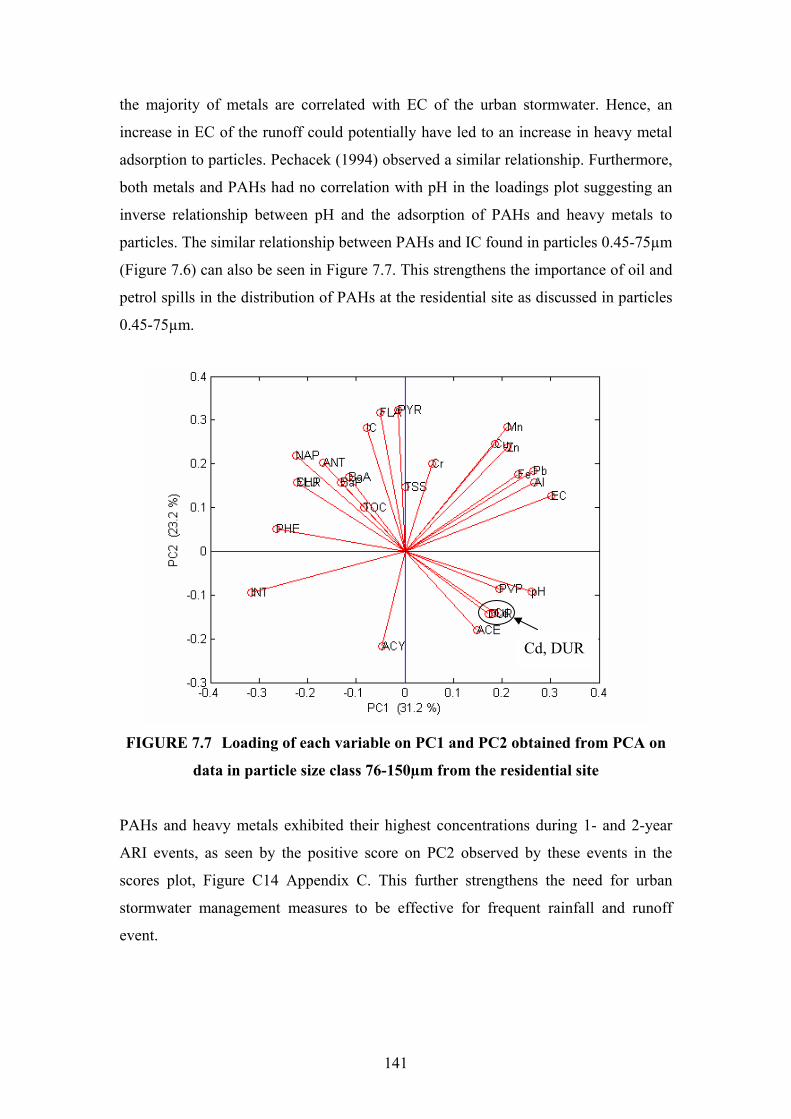
141
the majority of metals are correlated with EC of the urban stormwater. Hence, an
increase in EC of the runoff could potentially have led to an increase in heavy metal
adsorption to particles. Pechacek (1994) observed a similar relationship. Furthermore,
both metals and PAHs had no correlation with pH in the loadings plot suggesting an
inverse relationship between pH and the adsorption of PAHs and heavy metals to
particles. The similar relationship between PAHs and IC found in particles 0.45-75µm
(Figure 7.6) can also be seen in Figure 7.7. This strengthens the importance of oil and
petrol spills in the distribution of PAHs at the residential site as discussed in particles
0.45-75µm.
FIGURE 7.7 Loading of each variable on PC1 and PC2 obtained from PCA on
data in particle size class 76-150µm from the residential site
PAHs and heavy metals exhibited their highest concentrations during 1- and 2-year
ARI events, as seen by the positive score on PC2 observed by these events in the
scores plot, Figure C14 Appendix C. This further strengthens the need for urban
stormwater management measures to be effective for frequent rainfall and runoff
event.
Cd, DUR

142
Particle size class >150µm
Heavy metals and PAHs were less frequently detected in particles above 150µm
compared to finer particle size classes. This has been attributed to the relatively large
surface area of fine particles compared to coarse particles (Andral et al. 1999; Sartor
and Boyd 1972). Only eight of the 16 analysed PAHs were detected in this particle
size. The scree plot (Figure C15 Appendix C) revealed that three principal
components contained most of the data variance. However, adding a third component
to the loadings plot (refer to Figure C16 Appendix C) did not contribute to the
identification of processes responsible for the distribution of PAHs and heavy metals
in washed-off particles above 150µm.
FIGURE 7.8 Loading of each variable on PC1 and PC2 obtained from PCA on
data in particle size class >150µm from the residential site
Similar to the fine particle size classes at the residential site, the PAHs and heavy
metals are separated by negative (PAHs) and positive (heavy metals) loadings on
PC1, as can be seen in Figure 7.8. In spite of this, the processes governing the
distribution of PAHs and heavy metals in particles above 150µm are slightly different
to the finer particles. This is attributed to TOC being correlated with heavy metals in
particles above 150µm. This is contradictory to the results obtained for particles 76-

143
150µm, where the TOC was correlated with most of the PAHs. Hence, the PAHs and
heavy metals differ in sorption behaviour depending on particle size. This can be
attributed to a number of reasons. Firstly, there could be differences in the source of
the organic matter (DeWitt et al. 1992). Secondly, PAHs have been found to be
irreversibly bound to soot carbon content, which could have influenced the
relationship found between PAHs and TOC in particles 76-150µm (Gustafsson et al.
1997). Thirdly, variations in PAH binding to organic carbon have been found to be a
function of pH and temperature (Warren et al. 2003). Furthermore, TOC is correlated
to the EC of the stormwater as can be seen in Figure 7.8, which could adversely
influence the adsorption of PAHs. Warren et al. (2003) noted that less-polar organic
matter gives rise to a better environment for the sorption of PAHs. More importantly,
microbial degradation of the organic matter could lead to the release of metals into the
water column, which in turn could impose a significant threat to aquatic organisms
due to the increased bioavailability.
Similar to finer particles, the adsorption of heavy metals to particles above 150µm at
the residential site is dependent on the EC of the runoff water. Hence, a rise in EC of
the stormwater led to an increased amount of heavy metals adsorbing to particles
independent of its size. Additionally, pH displayed an inverse relationship with the
adsorption of PAHs and heavy metals to particles at the residential site. This is
contradictory to the results obtained by Tai (1991) who found that a rise in pH
favoured the adsorption of metals to particulates. However, the small changes in pH
observed at the residential site due to the fairly constant pH in the rainfall used for
simulating runoff makes it difficult to fully evaluate the influence of pH on the
sorption of pollutants.
The majority of PAHs detected in the specific particle size class were inter-related as
can be seen in Figure 7.8. PAHs were correlated with TSS concentrations suggesting
that they were strongly bound to particles in the specific size class. Consequently, the
PAHs in the specific particle size class were less susceptible to chemical distribution
processes. This is attributed to the characteristics of the sources available (Latimer et
al. 1990; Larkin and Hall 1998). The percentage of natural sources of PAHs could be
higher in residential areas due to the proximity to parklands and forests. More
importantly, urban stormwater management measures based on gravity settling have

144
the potential to remove a large percentage of the PAHs absorbed to particles above
150µm. Conversely, when compared to the concentrations and loads of PAHs that
could be introduced by particles below 150µm, only a small fraction of the total load
could be removed by gravity settling.
The intensity and duration of the rainfall had an insignificant effect on the wash-off of
PAHs and heavy metals adsorbed to particles above 150µm. Similar to fine particles
at the residential site, the more frequent events such as 1- and 2-year ARI events were
more important in the wash-off of PAHs and heavy metals. This is shown by the
positive score of 1- and 2-year events on PC2 as seen in the scores plot, in Figure C17
Appendix C.
7.5.2 Industrial site
Eleven runoff events were generated by the rainfall simulator at the industrial site.
Thus, eleven data objects for each fraction of the wash-off sample were analysed
using PCA.
Dissolved fraction (Particles <0.45µm)
Similar to the dissolved fraction of runoff at the residential site, PAHs were rarely
detected. Only six of the 16 analysed PAHs were detected. Three (Cr, Cd and Fe) of
the eight metal elements analysed were below detection limit in the dissolved fraction.
As shown by the scree plot, in Figure C18 Appendix C, three principal components
were preferred to interpret the results from the PCA. The three principal components
contained 78.2% of the data variance (46.3%, 21.2% and 10.7% respectively).
However, the three dimensional loadings plot (Figure C19 Appendix C) did not reveal
any additional information to the two-dimensional loadings plot (Figure 7.9). Hence, a
two-dimensional loadings plot of PC1 and PC2 was sufficient to visually explore the
results from the PCA.

145
FIGURE 7.9 Loadings of each variable on PC1 and PC2 obtained from PCA on
the dissolved fraction of wash-off from the industrial site
As can be seen in Figure 7.9, the PAHs and heavy metals were associated with
positive loadings on PC1, which suggests that similar processes were governing their
distribution in the dissolved fraction of runoff at the industrial site. These processes
were attributed to:
• Organic complexation;
• Increased adsorption affinity due to an increase in EC; and
• Inverse relationship with pH.
The primary process distributing the PAHs and heavy metals in the dissolved fraction
at the industrial site was the relationship with DOC. As can be seen in Figure 7.9, six
of seven detected PAHs (BaP, BgP, NAP, BaA, ACY and ACE) and two of the five
detected metals (Zn and Pb) in the dissolved fraction were correlated with DOC.
Furthermore, BaP, BgP and BaA were detected above their aqueous solubility during
the rainfall events. This is attributed to their correlation with DOC. Warren et al.
(2003) noted the solubility enhancement effect of PAHs when bound to dissolved
organic carbon. However, as Smith et al. (2000) noted, the excess concentrations of
PAHs in the dissolved phase can also be attributed to the common definition of the
ACE, ACY
BgP, NAP, Pb, Zn, DOC

146
aqueous phase. Consequently, sub-micron (<1μm) particles passing through a 0.45µm
filter could be responsible for the above aqueous PAH concentrations observed. In
spite of this, no correlation with dissolved solids (TDS) was found for the PAHs,
(except FLA) suggesting that the PAHs were in fact available in a ‘freely’ dissolved
phase and readily bioavailable. It is postulated that the colloidal organic matter has in
fact degraded through various biological activities and hence has brought the PAHs
into solution. Ellis and Revitt (1982) confirmed that biological activity could
decompose colloidal organic matter. However, PAHs in the dissolved phase are also
more susceptible to biodegradation processes such as photo oxidation (McGroddy et
al. 1996). Hence, a detention basin could potentially remove PAHs in the dissolved
phase if the stormwater is stored long enough.
A correlation between DOC and Zn has been found by several researchers (Qu and
Kelderman 2001; Sansalone and Buchberger 1997). This was attributed to the
removal of ionic Zn by organic complexation (Ellis et al. 1987). Additionally, the
majority of PAHs and heavy metals in the dissolved phase showed an inverse
relationship with the pH of the runoff. This was similar to the residential site and is
supported by findings by Tai (1991).
No correlation between PAHs, heavy metals and rainfall intensity could be observed
in the dissolved fraction at the industrial site. Independent of the rainfall intensity, the
positive loadings on PC1 coincided with positive scores on PC1 obtained by 1- and 2-
year design rainfall events with short durations as seen in the scores plot, Figure C20
Appendix C. Thus, higher pollutant concentrations were observed in frequent rainfall
events. It is also important to note that the pollutant load could potentially be higher in
a less frequent rainfall event due to the increased volume of runoff. Hence, measures
taken to improve or protect existing water quality should not be influenced by rainfall
characteristics such as rainfall volume, as often is the case when water quantity and
quality measures are combined.
Particle size class 0.45-75µm
Only one of the 16 priority PAHs was not detected in particle size 0.45-75µm at the
industrial site. The heavy metal concentrations detected in this particle size class were
the highest observed, which corresponded with the highest volume of particles.

147
Consequently, from an urban stormwater management perspective, this was the most
important particle size class at the site.
Most of the data variance could be explained by using two principal components, as
shown by the elbow occurring at PC2 in the scree plot, in Figure C21 Appendix C.
PC1 and PC2 contained 40.2% and 16.6% of the data variance respectively. As can be
seen in the loadings plot (Figure 7.10), Mn, Zn, Pb, Fe, Al and Cu were all correlated
to pH suggesting that an increase of the pH in the stormwater would increase the
metal concentrations. Hence, it is likely that an equivalent decrease in pH of the
stormwater could increase desorption of metals and bring them into solution
(<0.45µm). Similar results were found by Tai (1991). Hence, the relationship found
between pH and heavy metals in the 0.45-75μm particle size range could have serious
implications for the bioavailability of heavy metals reaching receiving waters.
Furthermore, the majority of metals were associated with TSS and PVP of the
particles. Hence, a significant metal load was carried by surface runoff from the
industrial site.
FIGURE 7.10 Loadings of each variable on PC1 and PC2 obtained from PCA on
particles 0.45-75µm in wash-off from the industrial site
PC1 (40.2%)
PC2
(16.
6%)
PHE, ACE
Zn, Mn, Fe, Pb
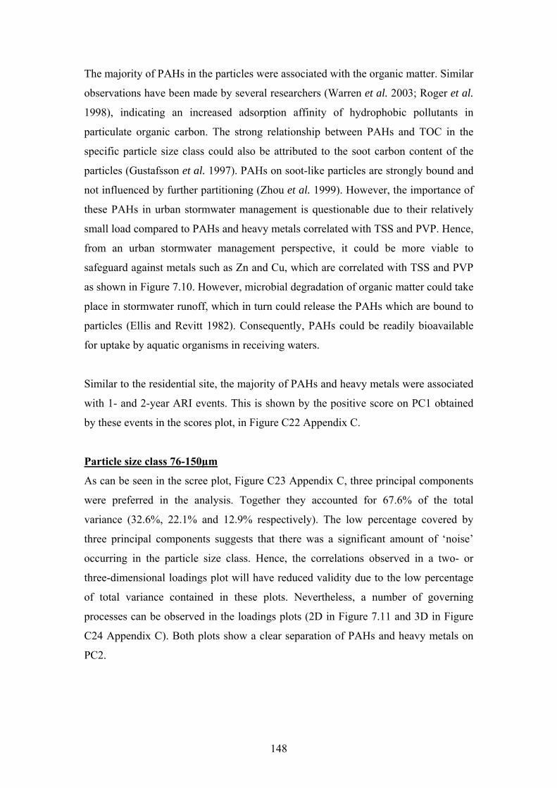
148
The majority of PAHs in the particles were associated with the organic matter. Similar
observations have been made by several researchers (Warren et al. 2003; Roger et al.
1998), indicating an increased adsorption affinity of hydrophobic pollutants in
particulate organic carbon. The strong relationship between PAHs and TOC in the
specific particle size class could also be attributed to the soot carbon content of the
particles (Gustafsson et al. 1997). PAHs on soot-like particles are strongly bound and
not influenced by further partitioning (Zhou et al. 1999). However, the importance of
these PAHs in urban stormwater management is questionable due to their relatively
small load compared to PAHs and heavy metals correlated with TSS and PVP. Hence,
from an urban stormwater management perspective, it could be more viable to
safeguard against metals such as Zn and Cu, which are correlated with TSS and PVP
as shown in Figure 7.10. However, microbial degradation of organic matter could take
place in stormwater runoff, which in turn could release the PAHs which are bound to
particles (Ellis and Revitt 1982). Consequently, PAHs could be readily bioavailable
for uptake by aquatic organisms in receiving waters.
Similar to the residential site, the majority of PAHs and heavy metals were associated
with 1- and 2-year ARI events. This is shown by the positive score on PC1 obtained
by these events in the scores plot, in Figure C22 Appendix C.
Particle size class 76-150µm
As can be seen in the scree plot, Figure C23 Appendix C, three principal components
were preferred in the analysis. Together they accounted for 67.6% of the total
variance (32.6%, 22.1% and 12.9% respectively). The low percentage covered by
three principal components suggests that there was a significant amount of ‘noise’
occurring in the particle size class. Hence, the correlations observed in a two- or
three-dimensional loadings plot will have reduced validity due to the low percentage
of total variance contained in these plots. Nevertheless, a number of governing
processes can be observed in the loadings plots (2D in Figure 7.11 and 3D in Figure
C24 Appendix C). Both plots show a clear separation of PAHs and heavy metals on
PC2.
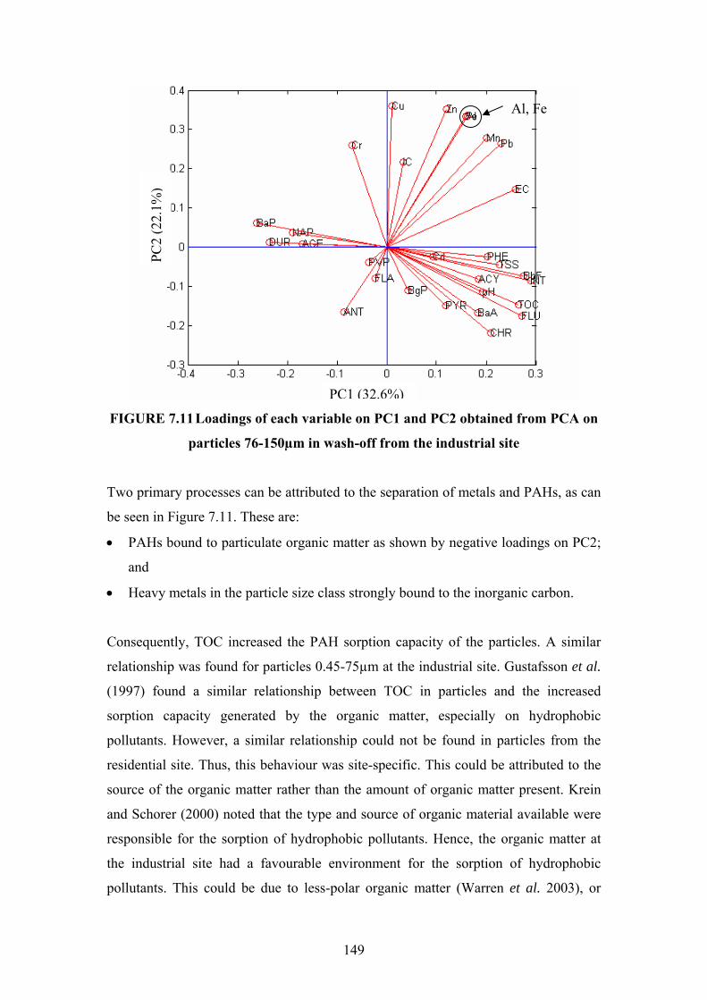
149
FIGURE 7.11 Loadings of each variable on PC1 and PC2 obtained from PCA on
particles 76-150µm in wash-off from the industrial site
Two primary processes can be attributed to the separation of metals and PAHs, as can
be seen in Figure 7.11. These are:
• PAHs bound to particulate organic matter as shown by negative loadings on PC2;
and
• Heavy metals in the particle size class strongly bound to the inorganic carbon.
Consequently, TOC increased the PAH sorption capacity of the particles. A similar
relationship was found for particles 0.45-75µm at the industrial site. Gustafsson et al.
(1997) found a similar relationship between TOC in particles and the increased
sorption capacity generated by the organic matter, especially on hydrophobic
pollutants. However, a similar relationship could not be found in particles from the
residential site. Thus, this behaviour was site-specific. This could be attributed to the
source of the organic matter rather than the amount of organic matter present. Krein
and Schorer (2000) noted that the type and source of organic material available were
responsible for the sorption of hydrophobic pollutants. Hence, the organic matter at
the industrial site had a favourable environment for the sorption of hydrophobic
pollutants. This could be due to less-polar organic matter (Warren et al. 2003), or
PC1 (32.6%)
PC2
(22.
1%)
Al, Fe

150
PAHs being irreversibly trapped in soot-like carbon particles that are not subject to
further interaction (Zhou et al. 1999). In spite of this, it is important to note that a
number of individual PAHs did not show any correlation with TOC. These were
primarily 2- and 3-ring PAHs correlated with PVP. Hence, the total load of 2- and 3-
ring PAHs could potentially be higher in urban stormwater. Nevertheless, the
increased bioavailability of PAHs that can occur if the organic matter is decomposed
can have serious implications for the water quality.
It is hypothesised that minerals used in sheet metal production at the site, containing
metals such as Zn, Pb and Mn, were responsible for the association of metals with IC
in particles between 76-150μm at the industrial site as seen in Figure 7.11. Similar
results were found by Bertin and Bourg (1995) who suggested that metals were
attached to particles with inorganic support. However, this is contradictory to findings
by Ellis et al. (1986) and Droppo et al. (1998) who suggested that the organic fraction
plays a major role in partitioning of metals in stormwater. Furthermore, it is unlikely
that metals associated with sheet metal production should be distributed into a specific
particle size class. It is unclear why the metals were associated with IC in the specific
particle size class.
The heavy metals and PAHs in the loadings plot, in Figure 7.11 were also separated
by rainfall events. As can be seen in the scores plot, Figure C25 Appendix C, a
slightly negative score on PC2 is attributed to high intensity rainfall, which coincides
with the slightly negative load of INT in the loadings plot (Figure 7.11). This is
mirrored in the TSS concentration. A positive loading on PC2 is attributed to frequent
rainfall events such as 1- and 2-year events.
Particle size class >150µm
At the industrial site PAHs, were detected more frequently in particles above 150μm
compared to the residential site. Consequently, the reliability of observed
relationships between PAHs and other parameters was higher. Heavy metals were
frequently detected in the particles. As can be seen in the scree plot, in Figure C26
Appendix C, two principal components contained most of the data variance (35.6%
and 17% respectively).
151
The loadings plot (Figure 7.12) revealed several processes involved in distributing the
PAHs and heavy metals. The most prominent was the correlation between pH, EC and
a number of PAHs. Thus, an increase in pH and EC of the runoff increased the
adsorption affinity of particles above 150µm. Pechacek (1994) attributed the increase
in EC to the increase in the adsorption affinity of a particle. More importantly, a
decrease in pH or EC could potentially lead to an increased desorption of PAHs into
the water column. This would lead to an increased bioavailability of PAHs. However,
desorption of PAHs from particles would depend on factors such as the solubility of
the specific PAH and dissolved organic carbon present (Zhou et al. 1999).
FIGURE 7.12 Loadings of each variable on PC1 and PC2 obtained from PCA on
particles >150µm in wash-off from the industrial site
Cu and Cr are correlated with the IC of the particles, which is attributed to their
source specific input at the industrial site. Hence, Cu and Cr could be irreversibly
trapped in the crystal lattice of primary and secondary minerals (Charlesworth and
Lees 1999). However, metals such as Al and Fe are correlated with TSS and INT. It is
postulated that an appreciable amount of these metals is from eroded local soils,
which has been found to be a major contributor of Al and Fe in urban areas (Hopke et
al. 1980).
PC1 (35.6%)
PC2
(22.
1%)
EC, pH, ACY, BaA, BaP, CHR

152
7.5.3 Commercial site
At the commercial site, all 12 design rainfall events were simulated. The highest PAH
concentrations were recorded at this site, which was attributed to the land use
characteristics. Consequently, the higher source strength of PAHs at the commercial
site, due to the relatively high traffic volume, significantly influenced the PAH
concentrations.
Dissolved fraction (Particles <0.45µm)
Fifteen of the 16 PAHs listed by the US EPA (Manoli and Samara 1999) were
detected in the dissolved phase at the commercial site. This was attributed to
petrogenic sources such as oil and petrol spills. Moreover, the concentrations were
often well above the aqueous solubility of the PAHs. This was attributed to the
presence of oil and grease emulsions and colloidal size particles (Smith et al. 2000).
Nevertheless, the detection frequency was low for many PAHs, especially high-
molecular weight PAHs, making it difficult to investigate any PAH distribution
processes in the dissolved phase. Metals were detected in relatively low
concentrations in the dissolved phase. Cd and Cr were not detected in the dissolved
fraction.
As seen by the elbow in the scree plot Figure C28 Appendix C, most of the data
variance was contained in the three first principal components (44.3%, 19% and 9.6%
respectively). However, the third principal component contained less than 10% of the
total data variance. Hence, the use of two principal components was sufficient in the
analysis (Kaiser 1960). Furthermore, the three-dimensional loadings plot (Figure C29
Appendix C) contributed very little to the information that could be extracted from the
two-dimensional loadings plot (Figure 7.13).

153
FIGURE 7.13 Loadings of each variable on PC1 and PC2 obtained from PCA on
data in the dissolved fraction wash-off samples from the commercial site
As can be seen in the loadings plot, Figure 7.13, the solubility concentrations
observed for many of the PAHs are attributed to the correlation with DOC and TDS.
Hence, the presence of colloidal organic material enhanced the solubility of PAHs at
the commercial site (Warren et al. 2003). This relationship was strongest at the
commercial site, which corresponded with the highest concentrations of DOC
recorded for all the sites. Consequently, the amount of DOC available increased the
particulate/water interactions of PAHs. In spite of this, as Krein and Schorer (2000)
observed, the association between DOC and PAHs could also have been attributed to
the type and source of the organic matter. Additionally, Warren et al. (2003) noted
that the temperature of water could significantly increase the solubility of PAHs.
However, this was not investigated.
In conclusion, a number of factors were contributing to the elevated concentrations of
PAHs in the dissolved fraction at the commercial site. In addition, elevated
concentrations were associated with 1- and 2-year design rainfall events as seen by the
negative score of these events on PC2 in the scores plot Figure C30 Appendix C.
BaP, ACE, ACY, FLU, PHE, FLA, CHR, DOC, ANT
PYR, BgP, NAP

154
The dissolved metals at the commercial site did not show any correlation with
chemical parameters measured as seen in the loadings plot (Figure 7.13). However, an
inverse relationship with pH could be identified due to large angle between metal
elements and pH in the loadings plot. Due to small variations in pH of the runoff
water, it was difficult to validate the relationship with metals in the dissolved phase at
the commercial site.
The heavy metals in the dissolved fraction were associated with the lowest rainfall
intensity events simulated, as shown by the positive score of these events in the scores
plot, Figure C30 Appendix C. Due to the drop size and terminal velocity of the
different rainfall intensities being identical in the simulations, the sheet flow created
by the lowest rainfall intensity on the coarse textured surface at the commercial site
had to be insufficient to release particles embedded in the voids. Consequently, higher
rainfall intensities had a higher sediment/water concentration ratio of heavy metals.
Hence, dissolved metals were associated with the lowest rainfall intensity, which is
attributed to the coarse asphalt texture at the commercial site.
Particle size class 0.45-75µm
All 16 priority PAHs were frequently detected in particles at the commercial site.
Furthermore, all metals except Cd were detected in their highest concentrations in the
wash-off. Thus, the importance of safeguarding against this particle size class at the
commercial site is significant. As can be seen by the elbow or inflexion point in the
scree plot, Figure C31 Appendix C, three principal components were preferred to
investigate correlations and patterns. The three first principal components contained
34.7%, 26.0% and 9.2% respectively of the total data variance. As proposed by Kaiser
(1960), a component containing less than 10% of the total data variance contributes
very little to the reliability of the information that can be extracted from PCA. Hence,
it was decided to use two-dimensional plots in PCA interpretation. As seen by the
loadings plot, Figure 7.14, the majority of metals and PAHs have a positive loading
on PC1. However, they are quite clearly separated by PC2, where metals were
associated with positive and PAHs with negative loading. In addition to this, a number
of PAHs had a negative loading on PC1. The primary reason for the negative loading
on PC1 attributed to FLA, PHE and ANT was the correlation with IC. This
strengthens the hypothesis made from the residential data that petrogenic PAHs

155
containing inorganic carbon could have adsorbed to particles due to accidental spills.
Similar findings were noted by LaRiviere et al. (2003).
FIGURE 7.14 Loadings of each variable on PC1 and PC2 obtained from PCA on
particles 0.45-75µm in wash-off from the commercial site
The remaining PAHs are correlated with the TOC content of the particles,
strengthening the increased PAH adsorption affinity observed in organic particles by
Gustafsson et al. (1997) and Kleineidam et al. (1999). Consequently, a significant
amount of PAHs were transported by fine particles due to their affinity with TOC.
The metals attached to 0.45-75µm particles were not correlated with any chemical
processes at the commercial site, as seen in Figure 7.14. However, the correlation
between the majority of metals and Fe and Mn observed in Figure 7.14 could indicate
that the metals are bound to Fe and Mn oxides in particles, as found by Hamilton et al.
1984. This in turn would mean that the metals associated with Fe and Mn oxides were
scarcely available for release but could be susceptible to interactions by a pH change
(Charlesworth and Lees 1999).
IC, EC, pH, ANT, PHE
Mn, Zn, Pb, Al

156
Particle size class 76-150µm
As can be seen in the scree plot, in Figure C33 Appendix C, the reduction in the
gradient of the curve occurred at the fourth principal component. Hence, according to
Catell (1966), four principal components should be used to explore the data. However,
Kaiser (1960) recommended the use of the principal components containing more
than 10% of the total data variance for reliable interpretation of PCA. Consequently,
three principal components were used, which contained 31%, 24.7% and 15.8% of the
total variance respectively.
In spite of this, a visual comparison between the two- and three dimensional loadings
plots indicated that the three-dimensional plot (Figure C34 Appendix C) added very
little to the information that could be retained using a two-dimensional loadings plot.
Hence, the first two principal components were used to visually explore the scores
and loadings of the objects and variables respectively. As can be seen in the loadings
plot, Figure 7.15, most of the metals were inter-related. This is attributed to the strong
particulate bound Fe and Mn oxides occurring in the particles. Furthermore, similar
observations were found in particles 0.45-75µm, which suggests that binding to Fe
and Mn oxides is the dominant process amongst metals at the commercial site. It is
likely that the elevated EC found in the build-up sample at the site is partly
responsible for this behaviour due to the increased adsorption affinity attributed to a
rise in the EC (Pechacek 1994). However, sequential extraction of metals is needed to
further establish metals’ affinity with Fe and Mn oxides (Al-Chalabi and Hawker
1996). Similar to the finer particles at the site, the wash-off of metals from the street
surface is highest during the lowest intensity rainfalls investigated, as shown by the
positive score on both PC1 and PC2 obtained by 65 and 86mm/hr rainfall events
(refer to Figure C35 Appendix C). This is again attributed to the coarse surface texture
of the parking lot, which would embed an appreciable amount of fine particles in the
voids.

157
FIGURE 7.15 Loadings of each variable on PC1 and PC2 obtained from PCA on
particles 76-150µm in wash-off from the commercial site
PAHs in the specific particle size class showed somewhat different processes to PAHs
in particles 0.45-75μm. Only a few of the PAHs were correlated to TOC (FLA, FLU,
PHE). However, TOC concentrations were very low in the specific particle size and
on several occasions no organic carbon was detected at all, making it difficult to
evaluate the influence of TOC on heavy metals and PAHs. On the other hand, PAH
concentrations were highly affected by the pH and EC of the stormwater as seen in
Figure 7.15. Warren et al. (2003) has attributed this to the increase in electrostatic
charges on particle surfaces caused by an increase in EC and pH. They also noted that
these factors are much less significant than organic carbon content in determining the
distribution of PAHs. Consequently, the lack of organic carbon in the specific particle
size class could have led to the distribution of PAHs into particles occurring due to a
change in pH and EC. This highlights the number of chemical processes able to
govern the distribution of PAHs in urban runoff. Moreover, it highlights the need to
frequently monitor the chemical characteristics of urban stormwater in order to
efficiently mitigate the negative impacts on receiving waters these pollutants could
impose.
BbF, EC, pH, IND, PYR, ACE, ACY, BaA, BgP, BaP
Fe, Mn, Pb, Zn, Cu, Al
158
Particle size class >150µm
Similar to the particle size 76-150µm, the inflexion point of the scree plot occurred at
the fourth principal component suggesting the use of four principal components in
interpreting the PCA (Cattell 1966). However, only the three first principal
components contained more than 10% of the total variance. Hence, it was decided that
three principal components were sufficient to explore the PCA. The three first
principal component contained 38.0%, 20.0% and 13.2% of the total data variance
respectively.
The three-dimensional loadings plot can be found in Figure C37 Appendix C. Similar
correlations between variables were found in a two-dimensional loadings plot (Figure
7.16). Hence, the first two principal components contained much of the reliable
information. Similar correlations can be found in particles above 150µm, as was
found in finer particles. Hence, PAHs are correlated with TOC while the majority of
metals are strongly bound to Fe and Mn oxides. Consequently, the PAHs and metals
distributed in different particle sizes at the commercial site show similar distribution
processes independent of particle size.
However, the metals in the specific particle size class were also correlated with the pH
of the stormwater. Charlesworth and Lees (1999) noted that the carbonate fraction of
metals is susceptible to a change in pH. Hence, the metals could also have existed in
the carbonate fraction. This is supported by Al-Chalabi and Hawker (1996) who found
the carbonate fraction of metals to dominate in street dust in Brisbane, Australia. This
was attributed to street dust primarily consisting of soil materials. Consequently, an
appreciable amount of washed-off particles above 150µm could have originated from
the soil surrounding the site.

159
FIGURE 7.16 Loadings of each variable on PC1 and PC2 obtained from PCA on
particles >150µm in wash-off from the commercial site
As can be seen in Figure 7.16, INT and DUR were less important in the wash-off of
PAHs and metals in the specific particle size. Instead, more frequent rainfall events
such as 1- and 2-year events were associated with the wash-off of PAHs and heavy
metals. This observation is further strengthened by the positive score on PC1 obtained
by 1- and 2-year design rainfall events as shown in the scores plot, Figure C38
Appendix C.
7.6 Summary
The build-up and wash-off process kinetics of PAHs and heavy metals were
investigated using principal component analysis (PCA). Multivariate methods were
preferred due to the number of variables that could be analysed in order to understand
relationships between variables and objects. PCA was undertaken on the build-up and
wash-off samples separately. Furthermore, each particle size class was investigated to
determine the influence of particle size on chemical processes.
The results of the PCA of the build-up samples suggested a number of possible PAH
and metal sources and processes at the three study sites. It was found that vehicle
DbA, IND CHR, PYR, ACY
Zn, Al

160
traffic was a major contributor to the deposited material at all three sites. However, its
relative contribution was dependent on the site characteristics. Other sources included
gardening products and atmospheric deposition at the residential site, industrial
activities at the industrial site and accidental oil and grease spills at the commercial
site. The distribution of PAHs and heavy metals into particle size classes was similar
at the three sites, with the particle size class 0.45-75µm dominating. This was
consistently mirrored by the highest particle volume percentage (PVP) and total
suspended solids (TSS) concentrations being found in this size class. Consequently,
the PAHs and heavy metals found in the fine particles could have an adverse impact
on the water quality of receiving waters if incorporated into runoff. Therefore, urban
stormwater management measures should safeguard against fine particles independent
of land use characteristics.
No correlation was found between PAHs, metals and TOC in the build-up samples.
TOC was consistently found in relatively high concentrations in particles less than
0.45µm and particles above 150µm. These particle size classes were always low in
PAHs and heavy metals which made it difficult to investigate the influence of TOC on
PAHs and heavy metals in street deposited material. However, PAHs at the
commercial site were consistently found in concentrations above aqueous solubility in
particles below 0.45µm (referred to as the dissolved fraction) which was attributed to
two primary reasons. Firstly, a large number of oil and grease spills were observed
during sampling. Hence, PAHs absorbed to oil and grease emulsions could have led to
increased solubilities. Secondly, organic colloidal particles could have been
responsible for the solubilities recorded due to the increased adsorption affinity
observed in organic particles (Warren et al. 2003).
Mainly three different processes were governing the distribution of PAHs and heavy
metals. These were:
• Increased adsorption due to correlation with TOC;
• The association with IC; and
• Sediment binding on Fe and Mn oxides.
161
At the commercial and industrial sites, PAHs in the specific particle size class were
strongly bound to particles by the organic fraction. Nevertheless, at the residential site
and to some extent the commercial site, PAHs were primarily associated with
particles with an inorganic carbon support. This was attributed to the presence of
petrogenic sources at the residential and commercial sites. The PAHs bound to the
inorganic fraction were less susceptible to microbial degradation compared to the
organic fraction. However, the inorganic fraction was more susceptible to a change in
pH (Charlesworth and Lees 1999). Hence, processes such as acidic rainfall could
release the PAHs into the water column.
Processes governing the presence of metals in particles 0.45-75µm size class were
highly site specific. Factors such as soil composition, the presence of Fe and Mn-
oxides and pH of the stormwater were all important in partitioning the metals. More
importantly, it showed the wide range of factors that could partition metals in an
urban environment. Furthermore, it indicated the need for monitoring these
parameters in an urban area to ensure that urban stormwater management measures
are efficient in improving water quality.
In particles 76-150µm size, from the wash-off at the three sites, TOC and IC were
again dominating the distribution of PAHs and heavy metals. In spite of this, the
degree of influence differed between the sites. At the residential and commercial sites,
PAHs were correlated with TOC and to an extent IC, while at the industrial site PAHs
were strongly bound to the organic fraction of the particles. Similar to finer particles
at the commercial site, the metals were correlated with Fe and Mn, which was
attributed to the presence of Fe and Mn-oxides at the site.
Metals in particles above 150µm at the commercial site showed a similar distribution
to metals in the finer particles. Fe and Mn-oxides were governing the distribution of
metals independently into particle size classes in the wash-off from the commercial
site. At the industrial site, the presence of Cu and Cr in particles above 150μm was
attributed to industrial processes, due to their association with IC. At the residential
site, TOC was correlated with the majority of metals and the relationship was further
strengthened by an increase in pH. PAHs at the three sites were found in relatively
low concentrations in particles above 150µm size, especially at the industrial and
162
residential sites. However, when detected, they were correlated with an increase in the
pH or EC of the stormwater.
At all three sites, 1- and 2-year design rainfall events were the most important in
transporting PAHs and heavy metals. Consequently, relatively frequent events could
transport a significant pollutant load to receiving waters. Hence, combined water
quantity and quality measures could be inefficient in removing a large percentage of
the PAHs and heavy metals in urban runoff. Additionally, this highlights the
limitation of water quality approaches that has been based on water quantity research
undertaken in the past. Thus, the extension of such concepts and processes is not
satisfactory in urban water quality due to the strong reliance on physical factors and
the limited recognition of chemical processes.
The processes found in the respective size fractions in urban stormwater at the three
sites were considered transferable between the sites due to the reduced number of
physical factors involved in the runoff. However, to fully assess the transferability of
the processes and parameter relationships found, an approach needed to be undertaken
where the data set and processes could be calibrated and validated. According to
Wold et al. (2001), the flexibility of a PLS-approach and its ability to handle
incomplete and noisy data with many variables, makes it a simple but powerful
approach for the analysis of complicated problems. Hence, the use of PLS in urban
water quality studies could significantly enhance the outcomes of the research, which
is discussed in Chapter 8.

163
Chapter 8 Investigating Process Kinetics of PAHs and heavy
metals using PCA and PLS
8.1 Introduction
Chapter 7 highlighted a number of processes common for the distribution of micro-
pollutants, which were independent of site characteristics. For example, PAHs were
found to be strongly bound to the organic fraction of particles at the three sites
depending on particle size. Furthermore, changes to the pH and EC of the stormwater
influenced the bioavailability of metals at the three sites. Knowledge of these
processes and the variables involved are the basis for urban stormwater management
for impact mitigation on receiving waters, and could be detrimental in the
development of more efficient strategies. A key issue in urban stormwater has been
the transferability of fundamental urban water quality concepts and relationships to
other areas. In addition to this, chemical processes are often neglected when build-up
and wash-off of PAHs and heavy metals are studied. Consequently, it became
important to validate the transferability of the chemical processes, by excluding
physical factors and land use characteristics. This was made using a predictive
modelling approach of the chemical processes. Multivariate regression techniques
were used to predict PAHs and heavy metals based on variables such as TOC and Fe
and Mn oxides at the three sites. The performance of the predictive relationships then
determined the transferability of relationships found between sites. However, it is
important to realise that the modelling approach was used to validate the parameter
relationships found and their transferability, not specifically model and predict the
parameter concentrations for determining urban water quality impacts.
During the PCA analysis discussed in Chapter 7, it became apparent that the build-up
process kinetics of PAHs and heavy metals was highly site-specific and reflected the
sources available in the urban environment. Due to the number of build-up samples
collected from each site and the highly site-specific processes identified, it was
decided that the prediction of process kinetics in the build-up samples separately was
inadequate. However, similar processes were found to govern the wash-off kinetics of
heavy metals and PAHs from each site. Hence, the wash-off process kinetics of PAH

164
and heavy metals were found to be less dependent on source strength and could be
predicted independent of site characteristics. Furthermore, it was decided that
including build-up samples in developing predictive relationships based on the
chemical and physico-chemical processes influencing PAHs and heavy metals,
despite their strong source dependency, could identify possible processes and
common distribution characteristics previously unidentified in the separate analysis of
the build-up samples.
Consequently, the multivariate analytical methods PCA and PLS was employed to
investigate if chemical processes, physico-chemical processes and parameters could
explain the distribution of PAHs and heavy metals in build-up and wash-off,
independent of land use and particle size class. Similar to Chapter 7, PCA was applied
to the samples collected from the rainfall simulation. However, the PCA described in
Chapter 7 identified processes by particle size and site characteristics. In the PCA
performed in this Chapter, the complete set of data from the three sites was used as
one single data matrix. Hence, no particle sizes or study sites were biased in the
analysis.
8.2 Application of PCA for prediction of heavy metals and PAHs
In order to establish and validate reliable relationships between variables, outliers in
the data had to be identified and removed. Thus, PCA (refer to Appendix C page 280
for algorithm) was applied to the complete set of data incorporating build-up and
wash-off sample results from each site and particle size class. The pollutant data was
separated into matrices as follows:
• Matrix A containing 175 objects (samples) and 15 variables (8 heavy metal
elements and 7 physico-chemical parameters); and
• Matrix B containing 140 objects (samples) and 22 variables (15 PAH compounds
and 7 physico-chemical parameters).
The objects (samples) in each matrix were numbered prior to applying PCA due to
visual aspects of scores and loadings plots. The object lists containing the
abbreviations for each object used in the analysis can be found in Appendix D Table
D1 (Matrix A) and Table D2 (Matrix B) respectively.

165
Matrix A – Heavy metal data
Most of the variance (73.6%) of the 175 objects containing heavy metal data
subjected to PCA was contained in the first three principal components (41.1%,
21.3% and 11.2% respectively), as shown by the elbow at the third principal
component in the scree plot, in Figure D1 Appendix D.
-8 -6 -4 -2 0 2 4 6-4
-2
0
2
4
6
8
001
002
003004
005
006
007008009
010
011012013014
015
016017
018
019
020
021
022023
024025
026027
028029
030
031032033034
035
036037038
039040
041
042043
044045
046047048
049
050
051
052
053
054
055
056057058
059060
061
062063 064
065
066
067
068069
070
071072
073074075
076077
078
079080
081082
083084085
086087
088089
090
091092
093094
095
096097
098
099100
101102
103
104105
106107108
109110
111112
113114115
116
117118119
120
121
122123124
125
126
127128129
130
131132133
134
135
136137138139
140
141142
143144
145
146147148149
150
151152
153154
155
156157158159
160
161162
163164
165
166167
168169
170
171172
173
174
175
PC1 (41.1 %)
PC
2 (2
1.3
%)
FIGURE 8.1 Scores plot of the objects (175 samples) containing heavy metal data
subjected to PCA
When plotting the scores of each object (samples) on the first two principal
components (PC1 and PC2), as illustrated in the scores plot in Figure 8.1, three
distinct clusters could be identified as outlined below:
• Cluster 1, containing heavy metal data in particles less than 0.45μm (dissolved
wash-off samples) from the three sites;
• Cluster 2, containing heavy metal data in the build-up samples independent of site
and particle size class; and
• Cluster 3, containing heavy metal data in particles above 0.45μm in wash-off
samples from the three sites.
CLUSTER 1
CLUSTER 2
CLUSTER 3
166
Cluster 1 (dissolved samples) and Cluster 3 (particulate samples) identified a clear
separation between distribution processes of heavy metals in the particulate and
dissolved phases of street wash-off. Similar results have been found by numerous
researchers (Warren et al. 2003; Gueguen and Dominik 2003). Consequently,
modelling wash-off process kinetics of heavy metals in total water samples
(particulate plus dissolved phase) can be misleading and lead to gross errors in the
prediction of concentrations. Unfortunately, countless studies have investigated wash-
off of heavy metals using bulk samples (Drapper et al. 2000; Gray and Becker 2002;
Hoffman et al. 1984). Hence, the reliability of these studies in terms of best
management practises for urban stormwater is limited and the results from such
studies should be interpreted carefully. Similarly, there was a clear separation between
Cluster 2 containing the build-up samples and Cluster 1 and 3, which contained wash-
off samples. Furthermore, it can be observed in Figure 8.1 that the objects in Cluster 2
were scattered to some extent. This strengthens the strong site characteristic behaviour
intrinsic to the heavy metal compounds found in street dust, as discussed in Chapter 7.
Similar separations can be found when plotting the scores of the metal data objects on
a PC1 vs PC3 scores plot, as can be seen in Figure D2 Appendix D. However,
complementary information to the PC1 vs PC2 scores plot (Figure 8.1) can be found.
This is attributed to the separation of Cluster 3 (refer to Figure 8.1) on PC3.
Approximately half of the data objects in Cluster 3 had a positive score on PC3 while
the other half had a negative score on PC3. Hence, two primary wash-off processes
were separating the metal data in particles on PC3. As can be seen in the loadings plot
in Figure D3 Appendix D (PC1 vs PC3), the negative score was primarily attributed to
the presence of Fe and Mn oxides binding metals such as Al and Pb, while a positive
score indicated an association between Cu, Cd and Cr and the organic fraction of the
particles. Additionally, the loadings plots of PC1 vs PC3 and PC1 vs PC2 (Figures D3
and D4 Appendix D respectively) clearly separated Zn from the other metals. This
was attributed to Zn primarily being found in the dissolved phase, due to its
association with DOC and TDS independent of site characteristics, as discussed in
Chapter 6 and 7. Consequently, it was postulated that Zn could be predicted based on
DOC and TDS using the data from the dissolved samples at each site. Furthermore,
Chapter 7 identified the decrease in pH as a possible process influencing desorption of
167
heavy metals from particles. This was supported by Tai (1991) who found that the
desorption ratio of Zn increased when there was a decrease in pH. Therefore, it was
decided to include pH in the prediction of Zn (refer to Section 8.3) in the dissolved
fraction of runoff.
The remaining metals to be predicted were separated into two groups, based on the
outcome of the PCA. Hence, metals associated with Fe and Mn oxides were predicted
separately from the metals associated with the organic fraction of the particles, based
on the scores and loadings plots of PC1 vs PC3 (Figures D2 and D3 Appendix D
respectively). Additionally, only objects associated with each group and positive score
on PC1 were used in the prediction. Hence, objects with a positive score on PC3 were
used to predict metals associated with Fe and Mn oxides, while objects with a
negative score on PC3 were used to predict metals associated with the organic
fraction. The objects with negative and positive score on PC3 and the variables
associated with them are shown in Table 8.1. Refer to Table D1 Appendix D for
identification of site, runoff event and particle size class of each object.
As can be seen in Table 8.1, metals associated with Fe and Mn oxides were
dominating at the commercial site (objects 111-175), while the metals in the particles
collected at the industrial and residential site were primarily related to the organic
fraction of the particles. This behaviour was independent of particle size at the three
different sites, suggesting that binding to different fractions of particles was a site-
specific phenomenon. However, this does not exclude metals at the commercial site
from binding to the organic fraction of particles. On the contrary, metals at the
commercial site could very well be bound to the organic fraction of the particles.
Nevertheless, as Al-Chalabi and Hawker (1996) noted, the percentage of particles
with organic support could be significantly lower compared to the Fe and Mn oxides,
which in turn would influence a metal’s affinity with particle fraction. To fully assess
the fractionation of metals in washed-off particles, a number of extraction procedures
needs to be undertaken.
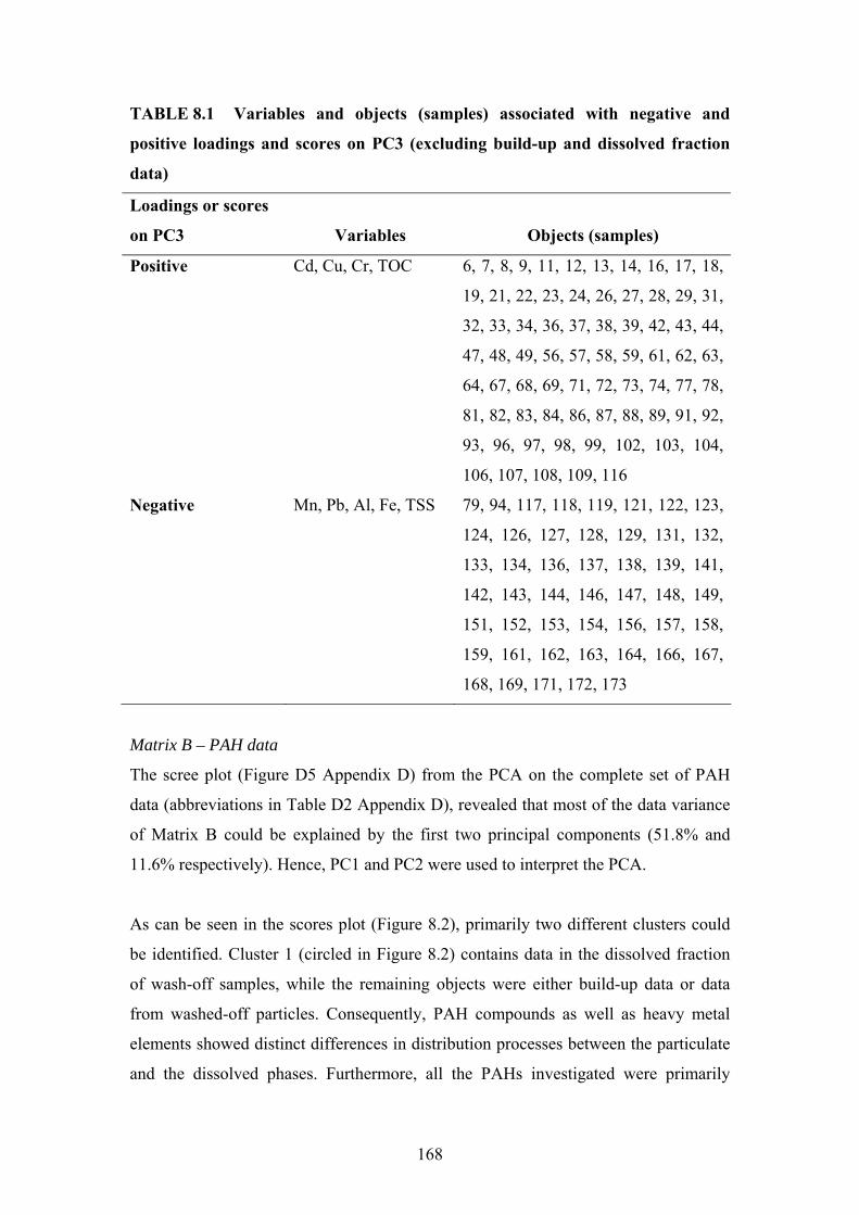
168
TABLE 8.1 Variables and objects (samples) associated with negative and
positive loadings and scores on PC3 (excluding build-up and dissolved fraction
data)
Loadings or scores
on PC3 Variables Objects (samples)
Positive Cd, Cu, Cr, TOC 6, 7, 8, 9, 11, 12, 13, 14, 16, 17, 18,
19, 21, 22, 23, 24, 26, 27, 28, 29, 31,
32, 33, 34, 36, 37, 38, 39, 42, 43, 44,
47, 48, 49, 56, 57, 58, 59, 61, 62, 63,
64, 67, 68, 69, 71, 72, 73, 74, 77, 78,
81, 82, 83, 84, 86, 87, 88, 89, 91, 92,
93, 96, 97, 98, 99, 102, 103, 104,
106, 107, 108, 109, 116
Negative Mn, Pb, Al, Fe, TSS 79, 94, 117, 118, 119, 121, 122, 123,
124, 126, 127, 128, 129, 131, 132,
133, 134, 136, 137, 138, 139, 141,
142, 143, 144, 146, 147, 148, 149,
151, 152, 153, 154, 156, 157, 158,
159, 161, 162, 163, 164, 166, 167,
168, 169, 171, 172, 173
Matrix B – PAH data
The scree plot (Figure D5 Appendix D) from the PCA on the complete set of PAH
data (abbreviations in Table D2 Appendix D), revealed that most of the data variance
of Matrix B could be explained by the first two principal components (51.8% and
11.6% respectively). Hence, PC1 and PC2 were used to interpret the PCA.
As can be seen in the scores plot (Figure 8.2), primarily two different clusters could
be identified. Cluster 1 (circled in Figure 8.2) contains data in the dissolved fraction
of wash-off samples, while the remaining objects were either build-up data or data
from washed-off particles. Consequently, PAH compounds as well as heavy metal
elements showed distinct differences in distribution processes between the particulate
and the dissolved phases. Furthermore, all the PAHs investigated were primarily

169
associated with particles in the wash-off samples as can be seen in the biplot, in
Figure D6 Appendix D. This is not surprising since PAHs have been found to be
primarily associated with the particulate fraction in urban stormwater (Marsalek et al.
1997). However, as identified in Chapter 7, PAHs could be present in the dissolved
fraction of runoff as oil and grease emulsion or attached to colloidal organic particles.
Nevertheless, the solubility of PAHs is low and it was decided to focus on predicting
PAHs in particles, due to the relatively higher PAH load that particles can transport to
receiving waters, compared to PAHs in the dissolved fraction. In addition, the
detection rate of PAHs in the dissolved fraction was low, which could influence the
accuracy of prediction significantly. As a result, it was decided to focus on the PAHs
found in particles.
Figure 8.2 also identified object outliers to have significantly larger scores on PC1
than other objects. These objects were identified as the build-up samples from each
site. Similar to the PCA of Matrix A, the build-up samples did not cluster closely in
the scores plot, which further strengthened the highly site specific nature of the build-
up of heavy metals and PAHs as identified in Chapter 7. Consequently, the presence
of PAHs and heavy metals in road-deposited material at the three sites was highly
source dependent. Similar results have been found by Sartor and Boyd (1972). The
higher presence of traffic-related PAHs in the build-up sample at the commercial site
is shown in Figure 8.2, where for example object number 91 (Commercial build-up
particle size range 0.45-75μm) had a significantly higher score on PC1 than objects 43
and 3, which were the corresponding build-up samples from the industrial and
residential sites.
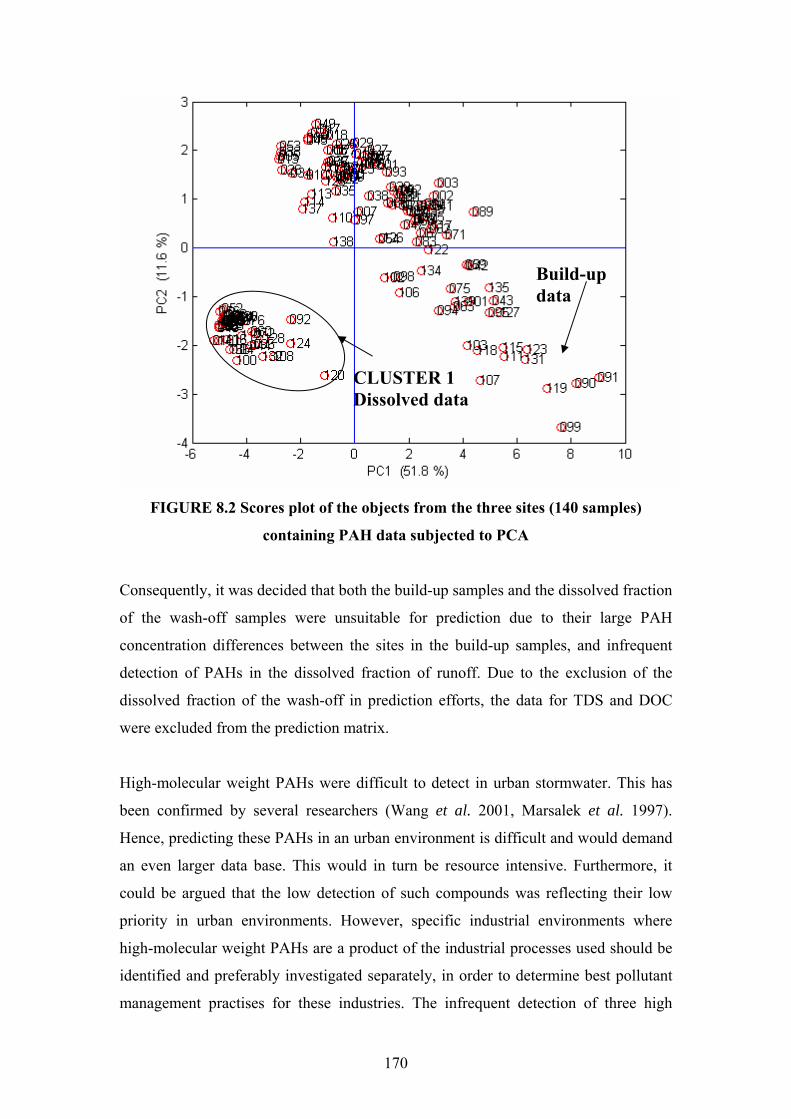
170
FIGURE 8.2 Scores plot of the objects from the three sites (140 samples)
containing PAH data subjected to PCA
Consequently, it was decided that both the build-up samples and the dissolved fraction
of the wash-off samples were unsuitable for prediction due to their large PAH
concentration differences between the sites in the build-up samples, and infrequent
detection of PAHs in the dissolved fraction of runoff. Due to the exclusion of the
dissolved fraction of the wash-off in prediction efforts, the data for TDS and DOC
were excluded from the prediction matrix.
High-molecular weight PAHs were difficult to detect in urban stormwater. This has
been confirmed by several researchers (Wang et al. 2001, Marsalek et al. 1997).
Hence, predicting these PAHs in an urban environment is difficult and would demand
an even larger data base. This would in turn be resource intensive. Furthermore, it
could be argued that the low detection of such compounds was reflecting their low
priority in urban environments. However, specific industrial environments where
high-molecular weight PAHs are a product of the industrial processes used should be
identified and preferably investigated separately, in order to determine best pollutant
management practises for these industries. The infrequent detection of three high
CLUSTER 1 Dissolved data
Build-up data

171
molecular weight PAHs (detected in less than 75% of the wash-off samples) led to the
removal of DbA, IND and BgP in the prediction step. Following this, 96 data objects
remained from the original Matrix B with data in 15 variables.
Due to the strong correlation between most of the PAHs and the build-up samples
attributed to the less frequent detection in wash-off samples, it was decided to apply
PCA to the wash-off data separately. Hence, PCA was applied to the 96 objects and
15 variables remaining in order to associate PAHs with specific objects and variables.
This resulted in most of the variance being accounted for in the first two principal
components, 41.0% and 11.3% respectively. This is strengthened in the scree plot, in
Figure D7 Appendix D, where the gradient of the curve flattens out at the second
component. The biplot (Figure D8 Appendix D) from the analysis confirmed the
higher strength of PAHs in the industrial and commercial wash-off samples, as seen
by the negative score obtained by the majority of residential wash-off samples on
PC1. Additionally, the objects with a negative score on PC1 represented PAH data in
particles above 150μm. This strengthens the findings in Chapter 7 where PAHs were
primarily associated with fine particles independent of particle size. Furthermore, the
majority of PAHs show no correlation with TOC in Figure D8 Appendix D. This is
contradictory to the analysis of the individual sites where TOC and PAHs were highly
correlated in fine particles. However, the TOC content was relatively high at all the
sites in particles above 150μm. Consequently, the relatively high TOC concentrations
recorded in the coarse particles skewed the loading of TOC on PC1 in the biplot, in
Figure D8 Appendix D. This shows the importance of analysing separate particle sizes
in urban water quality research since relevant information can be lost when analysing
bulk runoff samples. This is supported by findings by Smith et al. (2000) and Warren
et al. (2003), who suggested partitioning of runoff samples was preferable when
investigating urban water quality. As a result, no variables were left out of the
prediction of PAHs.
In addition, the biplot in Figure D8 Appendix D identified co-linearity between the
majority of PAHs. Hence, it became apparent that predicting individual PAHs
separately would produce the same information as using surrogate groups of PAHs in
a predictive relationship. For example, Figure D8 Appendix D identified co-linearity
between ACY, ACE and BbF based on the small angle separating their loadings in the

172
biplot (Kokot et al. 1998). Hence, a separate prediction for each of these groups
would produce a similar result, due to their distribution processes being similar.
However, PC1 and PC2 only accounted for 52.3% of the total data variance.
Therefore, the third principal component (9.2%) was considered statistically
significant in this case. By plotting the loadings of the PAH data on PC1 and PC3, as
shown in the loadings plot Figure D9 Appendix D, it was found that similar co-
linearity was occurring on PC3. However, two PAHs were not consistent in their
clustering on the three principal components analysed and showed an association with
different groups of PAHs, depending on the number of principal components used.
These were BbF and ANT, which consequently were excluded from the prediction
step. Based on the loadings on PC1, PC2 and PC3, the PAHs were separated into
three groups. These were:
• Group 1 (FLA and PYR);
• Group 2 (ACE and ACY); and
• Group 3 (FLU, PHE, NAP, BaP, BaA, CHR).
Hence, three different predictive parameter relationships were established based on
similar wash-off process kinetics of the PAHs attached to particles at the three
different study sites.
8.3 Introduction to PLS
Partial least square (PLS) regression is a generalisation of the more common multiple
linear regression (MLR). However, unlike MLR, PLS regression has the ability to
analyse data that is strongly collinear and noisy. PLS regression uses numerous X-
variables (in this research parameters such as pH, EC and TOC) in order to
simultaneously predict one to several response Y-variables (Wold et al. 2001). The
response of the Y-variables are then compared to observed values in a predicted
versus observed plot of the variable. Each Y-variable predicted is iteratively estimated
as the slope of a simple bivariate regression (least squares) between a matrix column,
or row. One way to see PLS regression is that it forms new X-variables as linear
combinations of the old and thereafter predicts a Y-variable based on these new X-
variables (Wold et al. 2001). Only as many new X-variables are formed as are needed.
Consequently, the significance of the prediction is always high. In order to interpret
the PLS prediction, loadings and scores are given to each variable which contain

173
information about the objects and their similarities/dissimilarities with respect to the
given problem. Hence, the loadings give information on how the variables combine to
form the quantitative relation between X and Y. Furthermore, they are essential in
understanding which X-variables are important in the prediction. The mathematical
formulation of PLS is given in Appendix D page 315.
In this research, PLS was particularly useful in order to predict a number of PAHs and
heavy metal elements using estimates of latent variables. Hence, chemical and
physico-chemical parameters was used as predictor variables X (such as TDS, pH and
DOC) which were used to predict selected response variables (Y), such as Zn. This
yielded information on the transferability of the research, as well as potential to
significantly influence current urban stormwater management practises.
There are a number of ways to determine the appropriate number of latent variables to
use in PLS regression. The X-scores are generally optimised and represented by the
least amount of orthogonal factors or latent variables, which provide minimal error in
the model. The PLS algorithm uses these scores and develops error predictions based
on calculated reduced eigenvalues (or error of calibration), cross-validation (Standard
Error of Validation (SEV) or predicted residual error sum of squares (PRESS).
PRESS is generally used to predict the number of latent variables to use when a
separate validation set is used. Furthermore, it is important to know something about
specifying errors in the quantification of the relationships. In multivariate analysis,
errors are usually quoted as the Standard Error of Prediction (SEP), which is
calculated from the square root of the sum of squared deviations between the
predicted and the actual concentrations. Hence, SEP should be similar to the standard
deviation for analyte concentrations and was an important parameter in determining
the transferability of the relationships found. Consequently, the lower SEP, the better
prediction.
There are two common forms of PLS typically employed. These are the PLS1 and
PLS2 routines (Wold et al. 2001). PLS1 are commonly used to predict singular Y-
variables, while PLS2 are utilised to predict several Y-variables at the same time.
Both algorithms have been successfully used to predict concentrations of variables
such as PAHs and dissolved organic carbon in water (Ferrer et al. 1998; Marhaba et

174
al. 2003). However, PLS1 was proven more effective than PLS2 in predicting PAHs
due to each compound being treated individually (Ferrer et al. 1998). Furthermore, as
noted by Beltran et al. (1998), the PLS2 algorithm did not improve the results
obtained by the PLS1 algorithm when predicting PAH concentrations. Thus, the
primary advantage with the PLS2 algorithm is the time saved when predicting several
compounds simultaneously.
In this research, a PLS1 algorithm was chosen primarily to predict the processes and
facilitate transferability of the relationships found. Loadings of each variable used in
the prediction could then be determined and the transferability of the parameter
relationships was based on the linear variation (r2) of the predicted variable (Y), and
the SEP. A step-by-step description of the algorithm is provided in Appendix D page
316, together with the functions used in the prediction. The software used was
MatLab and the algorithms cited were adapted from Mathisen (2004).
8.4 Predicting heavy metals and PAHs using PLS1 algorithm
Following the selection of suitable samples and variables for parameter prediction as
outlined in Section 8.2, a PLS1 algorithm was applied to the remaining PAH and
heavy metal data. The PLS1 algorithm was chosen due to the better performance
observed by a number of authors compared to multi-output processes (Ferrer et al.
1998; Dayal and MacGregor 1997). Additionally, as discussed in Section 8.2, the
majority of PAHs was strongly collinear. Hence, a specific PAH had been chosen as a
surrogate for a group of PAHs showing co-linearity. PLS1 is a quantification method
that uses a number of steps for creating a predictive relationship. These are:
1. The training (calibration) step;
2. The estimation (prediction) step; and
3. The validation step.
There are a number of options in the PLS analysis that needs to be discussed and
evaluated prior to regression can be undertaken. These options generally relate to the
validation of the developed relationships. There are primarily three different
validation options available. The first method is selecting half the objects available for
calibration and the other half for validation (Purcell et al. 2004). This method is useful
when a relatively large data set is available. In spite of this, a disadvantage with this

175
type of validation is that fewer objects are available for the calibration step, which
could significantly reduce the performance of the prediction. Thus, the model would
not contain as much predictive information as when the complete data matrix is used
for calibration. The second validation method is having a separate validation data set,
which will allow a more beneficial test of the overall efficiency. However, water
quality data available from the region had been collected on a catchment scale prior to
this research. Furthermore, concentrations had been measured in whole water samples
or dissolved and particulate form without further partitioning. Hence, the data
available was unsuitable for validating relationships based on data collected from a
small paved area, due to the amount of physical parameters influencing wash-off from
a mixed land use area. In addition to this, there was simply no time to collect a
sufficient set of data from natural rainfall during the timeline of the project. Hence,
using a separate validation data set with less detail relating to the distribution of heavy
metals and PAHs in particles was not valid.
In an ideal predictive model, as many calibration samples as possible should be
retained while at the same time being able to establish a realistic estimate for the
error. Thus, an error estimate that is truly indicative of the robustness of the
calibration is preferred. This can be achieved by a cross validation procedure, which
possesses many of the advantages of the conventional validation procedure, but does
not require samples to be sacrificed from the calibration set. This advantage is
achieved by leaving one sample out at the time in the validation procedure, which is
repeated until all samples have been left out of the calibration. The sample left out in
each step of the cross validation is used to gain an independent estimate of the error
for that particular sample. On the other hand, the cross-validation technique does not
allow for an estimation of the prediction error. Consequently, a predictive relationship
could be constructed using the cross-validation leave-one-out-method (Purcell et al.
2004). However, in terms of validation, a completely separate validation matrix is
needed. Therefore, it was decided to use half the objects in a cross validation
technique for calibration and use half the objects for validation. Performance of the
predictive relationship was then assessed from the value of the Standard Error of
Prediction (SEP). A similar technique has been successfully implemented by Purcell
et al. (2004).

176
8.4.1 Heavy metals in urban stormwater wash-off
The PLS1 algorithm (refer to Appendix D page 313) was used to predict a response
variable Y (heavy metal element) from numerous predictor variables X (TOC, TSS
and remaining metal elements due to Fe and Mn oxides and inter-correlations). The
metals were predicted using the following predictor variables, as outlined in Table
8.2, based on the outcomes of the PCA discussed in Section 8.2.
TABLE 8.2 Variables to be predicted (Y) and predictor variables (X) used
Y-variable X-variables
Pb Fe, Mn, TSS, pH, EC, IC
Cd TOC, pH, EC, IC
Cr TOC, pH, EC, IC
Zn DOC, TDS, pH, EC
Cu TOC, pH, EC, IC
Al TSS, Fe, Mn, pH, EC, IC
The concentrations measured in particles from the simulated runoff events were used
to predict the selected response variable as outlined above. Similar to PCA, the
concentrations of each variable were log transformed to reduce data heterogeneity.
Following this, the transformed data was column-centred and standardised in order to
reduce irrelevant sources of variation or noise. A calibration set was constructed by
selecting every odd numbered object (refer to Table 8.1) of the respective metal
groups. This resulted in three different calibration matrices depending on the metal
predicted. The calibration and validation matrix dimensions for each of the metal
groups (refer to Table 8.1) are outlined in Table 8.3.
TABLE 8.3 Calibration and validation matrices for prediction of metals
Metal elements
Calibration matrix
(objects x variables)
Validation matrix
(objects x variables)
Zn 16x4 16x4
Cu, Cr and Cd 37x4 37x4
Al and Pb 24x6 24x6

177
As discussed in Section 8.3, an important issue for any PLS approach is the number of
latent variables to be included. The number of latent variables to use was determined
when the prediction errors were minimised. Hence, the number of latent variables
corresponding to the first minimum in the cross-validation error plot was selected as
the optimum for prediction of the variables. As an example, the number of latent
variables used for the prediction of Cu was two, based on the first minimum in the
cross-validation error plot shown in Figure 8.3 below.
FIGURE 8.3 Cross-validation error (SEV) for Cu showing the number of latent
variables to use (2) based on the first minimum in the plot
The number of latent variables and their variance (proportion of variance obtained by
dividing the sum of squares of X by the corresponding total sum of squares of Y) for
each Y-variable to be predicted could thus be determined, and are shown in Table 8.4
below. Once the number of latent variables was determined, the X-scores were
recalculated to include the necessary information retained in the latent variables. As
can be seen by the percentage variance explained in Table 8.4, the latent variables
chosen contained the most variance in the data, with the majority of the remaining
variables made up of noise. Following this, the Y-variable was predicted and could be
compared to the original value in an observed versus predicted plot. Consequently, the
SEV
First minimum

178
higher the r2 value and the lower the SEP value, the better prediction and
performance.
TABLE 8.4 Number of latent variables used for each predicted variable (Y)
Y-variable Latent variables
Percentage variance
explained [%]
Pb 2 75.6
Cr 2 88.5
Zn 2 93.3
Cu 2 86.6
Al 3 79.4
Cd 2 82.8
As can be seen in the observed versus predicted plot Figure 8.4 below, the predicted
values of Al corresponded very well with the observed values of Al in washed-off
particles at all three sites (r2 = 0.90; SEP = 0.26).
FIGURE 8.4 Plot of observed versus predicted Al concentrations (logarithmic)
using three latent variables, with an SEP of 0.26
Observed Al concentrations log[mg/kg]
Pred
icte
d A
l con
cent
ratio
ns lo
g[m
g/kg
]
------ Predicted -- Observed
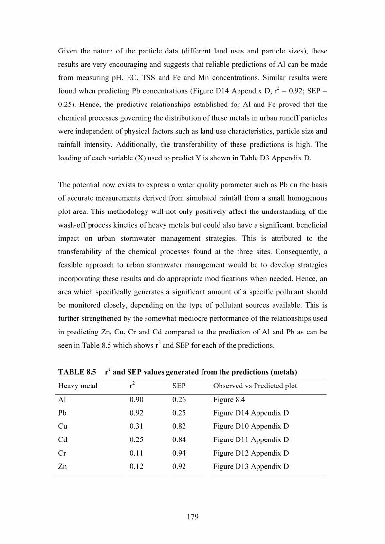
179
Given the nature of the particle data (different land uses and particle sizes), these
results are very encouraging and suggests that reliable predictions of Al can be made
from measuring pH, EC, TSS and Fe and Mn concentrations. Similar results were
found when predicting Pb concentrations (Figure D14 Appendix D, r2 = 0.92; SEP =
0.25). Hence, the predictive relationships established for Al and Fe proved that the
chemical processes governing the distribution of these metals in urban runoff particles
were independent of physical factors such as land use characteristics, particle size and
rainfall intensity. Additionally, the transferability of these predictions is high. The
loading of each variable (X) used to predict Y is shown in Table D3 Appendix D.
The potential now exists to express a water quality parameter such as Pb on the basis
of accurate measurements derived from simulated rainfall from a small homogenous
plot area. This methodology will not only positively affect the understanding of the
wash-off process kinetics of heavy metals but could also have a significant, beneficial
impact on urban stormwater management strategies. This is attributed to the
transferability of the chemical processes found at the three sites. Consequently, a
feasible approach to urban stormwater management would be to develop strategies
incorporating these results and do appropriate modifications when needed. Hence, an
area which specifically generates a significant amount of a specific pollutant should
be monitored closely, depending on the type of pollutant sources available. This is
further strengthened by the somewhat mediocre performance of the relationships used
in predicting Zn, Cu, Cr and Cd compared to the prediction of Al and Pb as can be
seen in Table 8.5 which shows r2 and SEP for each of the predictions.
TABLE 8.5 r2 and SEP values generated from the predictions (metals)
Heavy metal r2 SEP Observed vs Predicted plot
Al 0.90 0.26 Figure 8.4
Pb 0.92 0.25 Figure D14 Appendix D
Cu 0.31 0.82 Figure D10 Appendix D
Cd 0.25 0.84 Figure D11 Appendix D
Cr 0.11 0.94 Figure D12 Appendix D
Zn 0.12 0.92 Figure D13 Appendix D

180
Furthermore, as can be seen in Figures D10-D13 Appendix D (predicted versus
observed plots for Cu, Cd, Cr and Zn respectively), the predicted values did not
correspond very well with the observed values for these parameters. In the case of Zn,
which displayed relatively high concentrations in the dissolved fraction at the
residential site, this could be attributed to the presence of colloidal particles corroded
from galvanised roofs in the area. Makepeace et al. (1995) has confirmed corrosion
from galvanised roofs as an important source of Zn in an urban area. Thus, a point
source of a pollutant could significantly skew or bias prediction efforts and should
preferably be monitored separately. The majority of samples used in predicting Al and
Pb were from the commercial site. Hence, including additional samples from the
residential and industrial site could significantly skew the performance of the
prediction. To investigate the performance and further strengthen the transferability of
the established Al and Pb relationships, additional data from the residential and
industrial site were used. The results from the addition of data in predicting Al are
shown in Figure 8.5 below.
FIGURE 8.5 Plot of observed versus predicted Al concentrations when adding
additional samples from the commercial site, with an SEP of 0.56
Observed Al concentrations log[mg/kg]
Pred
icte
d A
l con
cent
ratio
ns lo
g[m
g/kg
]
------ Predicted -- Observed

181
As seen in Figure 8.5, the predictive performance of Al was still high when more
samples from the commercial site were added (r2 = 0.68; SEP = 0.56). Consequently,
the developed relationship based on Fe and Mn oxides in suspended solids proved the
transferability of the processes governing the distribution of Pb and Al between the
sites.
Additionally, as discussed in Chapter 7, the wash-off process kinetics of metals were
showing less trends and patterns between the three sites in less frequent storm events.
Thus, the importance of chemical processes could be more important in frequent
events and physical factors could potentially dominate in less frequent events. Hence,
the performance of the predictive relationships for Cu, Cr, Cd and Zn could have been
decreased due to the inclusion of less frequent events were the chemical processes
have a less dominating role in the distribution of metals. The Y-loading of each
variable is shown in Table D3 Appendix D.
8.4.2 PAHs in urban stormwater wash-off
As discussed in Section 8.2, the PAHs were split into three groups due to their distinct
co-linearity. Consequently, a surrogate PAH in each group was used to represent the
predictive performance of the PAHs belonging to the specific group. A PLS1
algorithm (refer to Appendix D page 313 for details) was used to predict the Y-
variables (PAH groups) based on a number of X-variables (TOC, IC, TSS, pH, EC).
Table 8.6 shows the Y-variables that were predicted and the predictor variables (X)
used.
TABLE 8.6 Variables to be predicted (Y) and predictor variables (X) used
Y-variable X-variables
Group 1 (FLA and PYR) TOC, IC, TSS, pH, EC
Group 2 (ACE and ACY) TOC, IC, TSS, pH, EC
Group 3 (FLU, PHE, NAP, BaP, BaA,
CHR)
TOC, IC, TSS, pH, EC
Similar to the prediction of heavy metals, a calibration and a validation matrix was
used for each PAH group. All three PAH groups to be predicted had calibration and

182
validation matrices consisting of 5 variables and 48 objects, and was chosen similar to
the calibration and validation matrices used in heavy metal prediction (refer to Section
8.4.1). The data was pre-treated prior to PLS application using column centering and
standardisation.
The number of latent variables was determined for each PAH group prior to the
prediction step. Hence, the cross-validation error for each Y-variable was determined
by visually inspecting the error plot and choosing the number of latent variables that
generated the smallest error for the calibration. The number of latent variables used
for each PAH group can be found in Table 8.7 below. It was observed that a different
number of latent variables were suggested for each PAH group. This was attributed to
the relatively low data variance accounted for in the first two principal components, as
discussed in Section 8.2. Hence, the addition of latent variables increased the
reliability and the performance of the prediction of PAH group 1 and 2. However, the
performance of the prediction of PAH group 3 was not affected by the addition of
latent variables. Following the determination of latent variables, new X-scores were
calculated in order to predict the PAH groups and loadings of each variable used to
predict the different PAH groups were calculated (refer to Table D3 Appendix D).
TABLE 8.7 Number of latent variables used for each predicted variable (Y)
Y-variable
Number of latent
variables
Percentage variance
explained [%]
Group 1 (FLA and PYR) 3 84.9
Group 2 (ACE and ACY) 4 76.5
Group 3 (FLU, PHE, NAP,
BaP, BaA, CHR)
2 87.4
As shown by the r2 values and SEP values of each of the predictions, Table 8.8, the
performance were reasonably good as indicated by the SEP.
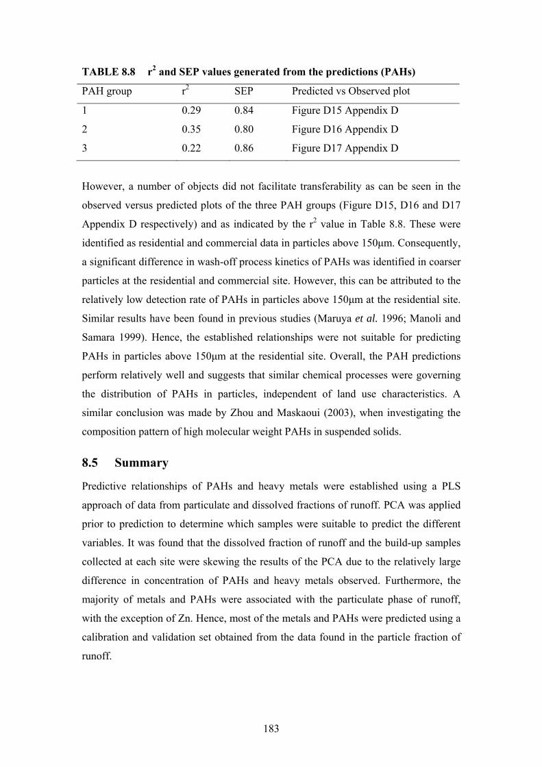
183
TABLE 8.8 r2 and SEP values generated from the predictions (PAHs)
PAH group r2 SEP Predicted vs Observed plot
1 0.29 0.84 Figure D15 Appendix D
2 0.35 0.80 Figure D16 Appendix D
3 0.22 0.86 Figure D17 Appendix D
However, a number of objects did not facilitate transferability as can be seen in the
observed versus predicted plots of the three PAH groups (Figure D15, D16 and D17
Appendix D respectively) and as indicated by the r2 value in Table 8.8. These were
identified as residential and commercial data in particles above 150μm. Consequently,
a significant difference in wash-off process kinetics of PAHs was identified in coarser
particles at the residential and commercial site. However, this can be attributed to the
relatively low detection rate of PAHs in particles above 150μm at the residential site.
Similar results have been found in previous studies (Maruya et al. 1996; Manoli and
Samara 1999). Hence, the established relationships were not suitable for predicting
PAHs in particles above 150μm at the residential site. Overall, the PAH predictions
perform relatively well and suggests that similar chemical processes were governing
the distribution of PAHs in particles, independent of land use characteristics. A
similar conclusion was made by Zhou and Maskaoui (2003), when investigating the
composition pattern of high molecular weight PAHs in suspended solids.
8.5 Summary
Predictive relationships of PAHs and heavy metals were established using a PLS
approach of data from particulate and dissolved fractions of runoff. PCA was applied
prior to prediction to determine which samples were suitable to predict the different
variables. It was found that the dissolved fraction of runoff and the build-up samples
collected at each site were skewing the results of the PCA due to the relatively large
difference in concentration of PAHs and heavy metals observed. Furthermore, the
majority of metals and PAHs were associated with the particulate phase of runoff,
with the exception of Zn. Hence, most of the metals and PAHs were predicted using a
calibration and validation set obtained from the data found in the particle fraction of
runoff.

184
The performance and reliability of some of the predictions strengthened the
hypothesis that chemical processes were transferable between the sites. Hence, by
reducing the number of physical factors in urban water quality studies, such as land
use characteristics and particle size, the transferability of fundamental concepts
become higher. This in turn could indirectly contribute to more effective urban
stormwater management, through the application of a more holistic approach.
However, there are a number of limitations to the established relationships even
though the methodology and processes used have been justified and validated. The
established relationships were aimed at validating the transferability process kinetics
of heavy metals associated with particles less than 300μm and could only predict
concentrations in this specific particle size class. Hence, “total” water concentrations
and heavy metal concentrations in particles above 300μm could not be predicted using
PLS with the established relationships. Only a small percentage (generally 10-15% of
total concentrations) of the investigated heavy metals was found in particles above
300μm. Similar results have been found by Liebens (2001) and Shinya et al. (2001)
indicating that metal concentrations increase with decreasing particle size. This is not
very surprising since finer particles have a higher sorption capacity and a relatively
larger surface area (Dong et al. 1984). More importantly, the majority of particles at
the three study sites were found to be fine particles. As a result, the majority of the
heavy metal pollutant load is carried by particles below 300µm which could have
serious implications for urban stormwater management.

185
Chapter 9 General Discussion
9.1 Rainfall simulation in urban water quality
Rainfall simulation was successfully used to simulate a number of design rainfall
events at three study sites in this research. The rainfall simulator developed was
highly portable due to its lightweight construction and easy assembly and provided
the user with maximum control over when, where and how rainfall was applied.
Consequently, it was a time and cost efficient method to create a database for urban
water quality research. However, a number of limitations were observed with rainfall
simulation and the use of a rainfall simulator, in reproducing natural rainfall
characteristics. These were:
• Limited ability to produce natural kinetic energy of rainfall;
• Intermittent rainfall compared to natural rainfall; and
• Limited drop size distribution.
Thus, it was important to realise that the rainfall simulator was not able to reproduce
rainfall characteristics perfectly. Furthermore, the rainfall simulator was specifically
developed to reproduce rainfall characteristics in the South-East Queensland region. It
is important to note that any developed rainfall simulator needs to be calibrated
accurately for the scope of the research.
The limitations noted above could therefore be reduced by accurately calibrating the
rainfall simulator for the conditions in which it will be used. One of the primary
objectives of this research was to reduce the number of physical parameters involved
in urban water quality. Therefore, the use of identical kinetic energy and drop size
distribution of the simulated rainfall events was preferable in this research. A change
in the water pressure entering the nozzles would change the drop size distribution and
hence the kinetic energy. Consequently, it is postulated that by changing water
pressure and oscillation cycles, rainfall events in regions all over the world could be
successfully simulated if the rainfall simulator is adequately calibrated for the
conditions in which it will be used.

186
9.2 Chemical processes
One of the primary objectives of this research was to identify the chemical process
inherent in pollutant build-up and wash-off as well as to reduce the number of
physical factors influencing urban water quality research. Hence, the transferability of
the research would be significantly improved compared to previous studies by the
improvement of methodology and reduction of physical factors used in the
investigation. Nevertheless, there were a number of limitations in the findings that are
important to discuss. Firstly, it was found that the type and source of chemical
pollutants, such as TOC, was influencing the distribution of PAHs and heavy metals
at the study sites. Consequently, the chemical processes for a number of individual
PAHs and metals were influenced by land use characteristics. In addition, this
relationship could differ between the particle size classes at an individual site.
However, an overall correlation was found between TOC and PAHs and metals at the
three study sites which suggested that the adsorption affinity of organic particles was
higher than other particulate fractions.
More importantly, DOC was found to influence the presence of PAHs and metals in
the dissolved phase of the wash-off samples. In spite of this, it was difficult to confirm
or predict this relationship, especially with PAHs, due to the low solubility of the
compounds investigated. It is recommended that future research focus specifically on
the relationship between PAHs, heavy metals and DOC and sampling and analytical
procedures suitable for such research are carefully chosen due to the low
concentrations expected in the dissolved fraction.
Thirdly, the influence of the pH and EC of the particles on the distribution of PAHs
and heavy metals was not investigated. This was due to the low amount of particles
obtained in the wash-off samples primarily due to the partitioning of the samples into
several particle size classes and the relatively small plot area. Hence, the methods
available for measuring pH and EC in particles were insufficient to adequately
determine the relative importance of these parameters in the partitioning of PAHs and
heavy metals. It is recommended that future research in urban water quality could
investigate the influence of the pH and EC of the particles on the adsorption of PAHs
and heavy metals.

187
It is also recommended that processes such as microbial degradation due to high
bacterial levels in the stormwater is investigated due to the negative impact it might
have on the efficiency of urban stormwater management. Furthermore, the impact of a
change in temperature on the wash-off process kinetics of PAHs and heavy metals
should be investigated.
9.3 Calibration of methodology
The parameter relationships and processes established in the research have served as a
baseline for the development of new effective urban stormwater management
strategies. The methodology used have significantly reduced the dependency of
natural rainfall and introduced a more generic approach to urban water quality
research. Furthermore, calibration and validation steps have been performed
throughout the research such as in the design of the rainfall simulator and the use of
design rainfall event as discussed in Chapter 3. Additionally, well known multivariate
methods have been used and the performance of the established relationships have
been calibrated and validated using well established techniques described in Chapter 7
and 8. Therefore, in view of the on-going calibration and validation of the research
methodology adopted throughout this research, significant reliance can be placed on
the outcomes derived.
9.4 Implications of chemical processes found
There are a number of important implications on urban stormwater management
measures that needs to be discussed from the findings of this research. At all three
sites, a relationship between heavy metals, PAHs and TOC were found. Even though
it differed with particle size primarily, due to the source of the organic matter and the
source of metal and PAHs, it can have serious implications for both the water quality
of receiving waters and measures implemented to reduce the impact of these
pollutants. This is attributed to a number of reasons such as:
• Microbial degradation of the organic matter could potentially release PAHs and
metals bound to the organic fraction into the water column;
• Increased bioavailability of PAHs and heavy metals which impose a significant
threat to aquatic organisms; and

188
• Increased mobility of PAHs and heavy metals due to organic matter being
correlated with fine particles.
The primary implications of these processes on urban stormwater management are:
• Limited efficiency of end of pipe solutions (retention/detention ponds, wetlands,
specific gross pollutant traps); and
• Limited efficiency of street sweeping due to the association with fine particulates.
Hence, more innovative solutions incorporating the chemical processes inherent to the
wash-off of PAHs and heavy metals are needed. The findings in this research suggest
the investigation of potential urban stormwater management measures for the
reduction of PAHs and heavy metals based on the chemical properties of the particles
and the water. This could be implemented with measures such as:
• More efficient street cleaning, primarily related to decreased release of fine
particles through the exhaust of street sweepers;
• Longer retention times of stormwater which could lead to an increased photo-
oxidation of PAHs;
• Fine solids separation; and
• Chemical treatment of stormwater.
Additionally, 1 and 2 year design rainfall events were carrying significantly higher
concentrations of PAHs and heavy metals at all three sites compared to 5 and 10 year
design rainfall events. This observation was independent of the rainfall intensity of the
design rainfall events. This highlighted the need for effective urban stormwater
management measures. Moreover, it was found during the prediction of PAHs and
heavy metals that the predictive performance decreased when 10 year design rainfall
events were incorporated. Thus, the chemical processes that were governing the wash-
off of PAHs and heavy metals became less significant in less frequent storms. The
physical processes of urban stormwater were more influential in 10 year design
rainfall events. The generic relationships derived are valid for other geographic
locations. However, the influence of rainfall intensities in different locations needs to
be understood prior to adopting the methodology and the derived relationships.

189
Chapter 10 Conclusions and Recommendations
10.1 Conclusions
Processes and concepts relating to urban water quality are well known in a qualitative
sense. However, their quantification has proven to be extremely difficult. This has
been a major failure in most research studies. Furthermore, the strong reliance on
physical factors and limited recognition of chemical processes in current urban water
quality studies have led to contradictory results reported and strong location specific
outcomes. Ultimately, this has led to limited knowledge on the process kinetics of
build-up, transmission and dispersion of PAHs and heavy metals. In order to obtain
sustainable urban stormwater management strategies, more scientifically robust
methodology in obtaining and analysing the data is needed. This is primarily
attributed to a multi-disciplinary approach where research methodologies adopted in
other areas should be considered. The main focus of this research project was to
develop a pragmatic approach for investigating the build-up and wash-off process
kinetics of PAHs and heavy metals on paved surfaces. The research aims and
objectives outlined in Chapter 1 were achieved through the development of three
primary processes. These were:
• The use of rainfall simulation in the investigation of chemical processes inherent
to urban water quality
It became apparent that the lack of control of physical factors in previous research
had significantly reduced the transferability of fundamental concepts in urban
water quality. Therefore, in an attempt to reduce or control the number of physical
factors involved, a rainfall simulator was developed and calibrated accurately for
the conditions on which it was used. Both the physical and chemical
characteristics of natural rainfall characteristics in the area were successfully re-
produced. The rainfall simulator, detailed in Chapter 3, provided satisfactory
control over a number of physical factors such as the duration and intensity of
rainfall and had the following characteristics:
o Ability to simulate rainfall intensities from approximately 10mm/hr up to
approximately 220mm/hr;
o Highly portable, not only from site to site but from plot to plot;

190
o Water efficient by re-using the water not sprayed on the research plot;
o Kinetic energy and drop size distribution similar to natural rainfall in
South-East Queensland; and
o Efficient runoff collection system for paved surfaces.
Furthermore, it generated an extensive data base suitable for undertaking urban
water quality research. Artificial rainfall was then applied to paved surfaces in
three different land uses, which were identified through investigations detailed in
Chapter 4. By using a homogenous plot area, the number of physical factors
involved in the wash-off process kinetics of PAHs and heavy metals was reduced.
This allowed for an in-depth investigation of the chemical processes inherent to
urban water quality.
• Identification of important particle sizes in urban stormwater management
The research undertaken strengthened the importance of fine particles in the
generation and transport of PAHs and heavy metals. This was achieved through
detailed laboratory tests on different particle size fraction of the build-up and
wash-off at the respective sites as discussed in Chapter 5 and 6. The methods
adopted were standard methods detailed by relevant authorities. Independent of
the land use, the highest concentrations of PAHs and heavy metals were
consistently found in particles 0.45-75µm. This was mirrored by the particle
volume percentage. Hence, priority should be given to the removal of fine
particles in urban stormwater to efficiently reduce pollutant loads reaching
receiving waters.
• Evaluation of important wash-off and build-up process kinetics using multivariate
analysis
The identification and recognition of important processes inherent to the
distribution of PAHs and heavy metals in the dissolved and particulate fraction of
runoff was resolved using multivariate analysis and appropriate laboratory
methodologies. The methodologies adopted were calibrated and validated step-by-
step as described in Chapter 5-7. Although multivariate methods have been
implemented by chemists to describe pattern recognition, classification and
191
prediction, it is rarely used in the engineering field even though it can provide
important information on relationships between variables which in turn could lead
to an increased knowledge of the processes involved. The use of multivariate
analysis significantly increased the information that could be obtained from the
collected data. This was primarily attributed to the ability to handle noisy and
collinear data. Chapter 5-7 goes through the data analysis in detail. The
investigations conducted were focused on a number of different fractions of the
build-up and wash-off. These studies involved extensive field investigations,
sampling and laboratory testing and detailed data analysis. The major findings
from the univariate and multivariate analysis of the build-up and wash-off samples
were:
o The adsorption and desorption of PAHs and heavy metals was primarily
related to type and amount of TOC present;
o Metals at the industrial site were trapped in mineral-like particles;
o PAHs were consistently found in concentrations above their aqueous
solubility which was attributed to the colloidal organic particles present
able to sorb hydrophobic pollutants;
o Depending on particle size class, the relationship between specific PAHs
and heavy metals with TOC differed;
o pH and EC influenced the desorption of PAHs and heavy metals from
particles;
o TSS was less important than chemical and physico-chemical parameters in
distributing the PAHs and heavy metals; and
o Rainfall intensity and duration was less important compared to chemical
and physico-chemical parameters in wash-off process kinetics of PAHs
and heavy metals.
Primary implications of these findings in urban stormwater management are:
o PAHs and heavy metals adsorbed to fine particles are easily transported in
urban stormwater, and hence impose a significant threat to receiving
waters and questions the use of conventional methods in removing
pollutants;
o PAHs and heavy metals could be released into a freely dissolved phase if
microbial degradation of the organic matter occur; and

192
o The efficiency of current urban management strategies based on gravity
settling could be significantly reduced if ‘hydrophobic friendly’ conditions
exist in fine particles.
• Validation of the transferability of parameter relationships
To facilitate transferability of processes inherent to urban water quality, predictive
relationships were established. This entailed the identification of key parameters
and key objects that were independent of physical characteristics such as land use.
This was achieved through the PLS approach, which was accurately calibrated and
validated as described in Chapter 8. The predictive relationships established
confirmed the importance of chemical processes in urban water quality and
suggested the processes identified could be transferable to different land uses.
Furthermore, the parameter relationships have the potential to be transferred to
different geographic location with slight modifications.
10.2 Recommendations
Although the developed methodology and established relationships has helped to
strengthen the knowledge of build-up and wash-off process kinetics in urban runoff,
there still remain a number of critical areas that have not been addressed through this
research. Therefore, it is recommended that further research is undertaken in the
following areas:
• The collection of more build-up samples from the sites in order to investigate the
importance of chemical processes in each particle size class. Only one build-up
sample was collected for each site in this research due to antecedent conditions
being kept identical for build-up and wash-off samples. It is recommended that the
influence of the antecedent dry period on the distribution of PAHs and heavy
metals in accumulated particles is investigated and any effect it may have on
chemical processes determined;
• Validation of the relationships and processes established in this research using
natural rainfall and runoff data. This primarily relates to establishing a sufficient
detailed data base for the validation of the chemical processes;

193
• Assessment of the role of suspended solids and dissolved organic carbon in urban
water quality. This issue has been addressed to some extent in this research but the
degradation of organic matter and the microbial activity of suspended solids are
important processes in urban water quality due to the increased bioavailability of
metals and PAHs this could cause. Hence, more detailed studies into the
adsorption and desorption of pollutants and its fate and transport once adsorbed or
desorbed could potentially improve the effectiveness of urban stormwater
management;
• The distribution of heavy metals and PAHs into different fractions, primarily
relating to difference in bioavailability. In this research, it was found that Al and
Pb were primarily bound to Fe and Mn oxides due to the correlation found in the
PCA. However, the partitioning of metals can occur in more fractions such as the
carbonate and exchangeable fraction. Furthermore, the percentage of metals
attached to the Fe and Mn oxide fraction was not determined. It is recommended
that future research could focus on determining the percentage of metals attached
to each fraction due to different sorption and desorption rates observed by
previous researchers between the fractions;
• Assessment of the influence of lower intensity rainfall on the wash-off of PAHs
and heavy metals from a paved surface. This is attributed to potential differences
in sorption and desorption of pollutants due to lower kinetic energy of rainfall.
Hence, the adsorption affinity of a suspended solid subjected to different kinetic
energies of rainfall should be investigated due to the potential difference in
mobility and bioavailability of pollutants. This was not investigated in this
research due to kinetic energy being kept constant during the simulated rainfall
events; and
• The influence of pH and EC of sediments on the adsorption of hydrophobic
pollutants. This is primarily attributed to the increased sorption kinetics of
particles due to changes in pH or EC observed by previous researchers.

194
References
1. Ahuja, L. R. (1990). Modelling soluble chemical transfer to runoff with
rainfall impact as a diffusion process. Soil Science Society of America
Journal, 54, 312-321.
2. Ahyerre, M., Chebbo, G., Tassin, B, and Gaume, E. (1998). Storm water
quality modelling, an ambitious objective?. Water Science and Technology,
37, 205-213.
3. Al-Chalabi, A.S., and Hawker, D. (1996). Retention and exchange behaviour
of vehicular lead in street dusts from major roads. The Science of the Total
Environment, 187,105-119.
4. Andral, M. C., Roger, S., Montrejaud-Vignoles, M., and Herremans, L.
(1999). Particle size distribution and hydrodynamic characteristics of solid
matter carried by runoff from motorways. Water Environment Research,
71(4), 398-407.
5. APHA (1999). Standard methods for the examination of water and
wastewater. American Public Health Association, American Water Works
Association, Water Environment Federation, Washington.
6. Arnaez, J., Larrea, V., and Ortigosa, L. (2004). Surface runoff and soil erosion
on unpaved forest roads from rainfall simulation tests in north-eastern Spain.
CATENA, 57(1), 1-14.
7. Assouline, S., and Mualem, Y. (1989). The similarity of regional rainfall: a
dimensionless model of drop size distribution. Transactions of the ASAE,
32(4), 1216-1222.

195
8. Assouline, S., El Idrissi, A., and Persoons, E. (1997). Modelling the physical
characteristics of simulated rainfall: a comparison with natural rainfall. Journal
of Hydrology, 196(1-4), 336-347.
9. AS/NZS (1998). Water Quality - Sampling - Guidance on the design of
sampling programs, sampling techniques and the preservation and handling of
samples. Report no 5667.1:1998, Australian Standards.
10. Bae, S.Y., Yi, S.M., and Kim, Y.P. (2002). Temporal and spatial variations of
the particle size distribution of PAHs and their dry deposition fluxes in Korea.
Atmospheric Environment, 35, 5491-5500.
11. Ball, J. E., Jenks, R., and Aubourg, D. (1998). An assessment of the
availability of pollutant constituents on road surfaces. The Science of the Total
Environment, 209(2-3), 243-254.
12. Ball, J. E. (2000). Runoff from road surfaces-How contaminated is it? Hydro
2000: 3rd international hydrology and water resources symposium of the
institution of Engineers, Australia, Perth, 259-264.
13. Beltran, J.L., Ferrer, R., and Guiteras, J. (1998). Multivariate calibration of
polycyclic aromatic hydrocarbon mixtures from excitation-emission
fluorescence spectra. Analytica Chimica Acta, 373, 311-319.
14. Bender, G. M., and Terstriep, M. L. (1984). Effectiveness of street sweeping
in urban runoff pollution control. The Science of the Total Environment, 33,
185-192.
15. Bertin, C., and Bourg, A.C.M. (1995). Trends in the heavy metal content (Cd,
Pb, Zn) of river sediments in the drainage basin of smelting activities. Water
Research, 29(7), 1729-1736.

196
16. Bertrand-Krajewski, J.-L., Chebbo, G., and Saget, A. (1998). Distribution of
pollutant mass vs volume in stormwater discharges and the first flush
phenomenon. Water Research, 32(8), 2341-2356.
17. Black, J. A. (1977). Types and sources of contaminants. Water pollution
technology, Reston Publishing Company, Inc, 99-109.
18. Bodo, B. A. (1989). Heavy metals in water and suspended particulates from an
urban basin impacting Lake Ontario. The Science of the Total Environment,
87/88, 329-344.
19. Bomboi, M. T. and Hernandez, A. (1991). Hydrocarbons in urban runoff: their
contribution to waste waters. Water Research, 25(5) 557-65.
20. Brezonik, P. L., and Stadelmann, T. H. (2002). Analysis and predictive models
of stormwater runoff volumes, loads, and pollutant concentrations from
watersheds in the Twin Cities metropolitan area, Minnesota, USA. Water
Research, 36(7), 1743-1757.
21. Bris, F.-J., Garnaud, S., Appery, N., Gonzalez, A., Mouchel, J.-M., Chebbo,
G., and Thevenot, D. R. (1999). A street deposit sampling method for metal
and hydrocarbon contamination assessment. The Science of the Total
Environment, 235, 211-220.
22. Bruwer, C. A. (1982). Water quality interactions of three successive urban
storms. Urban stormwater quality management and planning, B.-C. Yen, ed.,
Water Resources Publications, Urbana, Illinois USA, 10-18.
23. Bubb, J. M., and Lester, J. N. (1994). Anthropogenic heavy metal inputs to
lowland river systems, a case study. The river Stour U.K. Water, Air and Soil
pollution, 78, 279-296.
24. Bubenzer, G. D., and Meyer, L. D. (1965). Simulation of rainfall and soils for
laboratory research. Transactions of the ASAE, 8, 73-75.
197
25. Bubenzer, G. D. (1979a). Inventory of rainfall simulators. Rainfall simulator
workshop, Tucson, AZ, 120-130.
26. Bubenzer, G. D. (1979b). Rainfall characteristics important for simulation.
Rainfall simulator workshop, Tucson, AZ, 22-34.
27. Bucheli, T.D., Blum, F., Desaules, A., and Gustafsson, Ö. (2004). Polycyclic
aromatic hydrocarbons, black carbon and molecular markers in soils of
Switzerland. Chemosphere, 56, 1061-1076.
28. Butler, D., Thedchanamoorthy, S., and Payne, J.A. (1992). Aspects of surface
sediment characteristics on an urban catchment in London. Water Science and
Technology, 25, 13-19.
29. Carpenter, S. R., Caraco, N. F., Correll, D. L., Howarth, R. W., Sharpley, A.
N., and Smith, V. H. (1998). Nonpoint pollution of surface waters with
phosphorus and nitrogen. Ecological Applications, 8(3), 559-568.
30. Catallo, W. J., and Gambrell, R. P. (1987). The effects of high levels of
polycyclic aromatic hydrocarbons on sediment physico-chemical properties
and benthic organisms in a polluted stream. Chemosphere, 16(5), 1053-1063.
31. Cattell, R.B. (1966). The scree test for the number of factors. Multivariate
Behavioural Research, 1, 521-527.
32. Charlesworth, S.M., and Lees, J.A. (1999). The transport of particulate-
associated heavy metals from source to deposit in the urban environment,
Coventry, UK. The Science of the Total Environment, 235, 351-353.
33. Chiew, F. H. S., Duncan, H. P., and Smith, W. (1997). Modelling pollutant
build-up and wash-off: keep it simple. 24th International and Water Resources
Symposium, Auckland, 131-136.

198
34. Choi, W. W., and Chen, K. Y. (1976). Associations of chlorinated
hydrocarbons with fine particles and humic substances in near shore surficial
sediments. Environmental Science and Technology, 10(8), 782-786.
35. Christensen, E. R., and Guinn, V. P. (1979). Zinc from automobile tires in
urban runoff. Journal of the Environmental Engineering Division, ASCE,
105(EE1), 165-168.
36. Christiansen, J. P. (1942). Irrigation by sprinkling. Bulletin No 670, University
of California Agricultural Experiment Station.
37. Corbett, C. W., Wahl, M., Porter, D. E., Edwards, D., and Moise, C. (1997).
Nonpoint source runoff modelling: A comparison of a forested watershed and
an urban watershed on the South Carolina coast. Journal of Experimental
Marine Biology and Ecology, 213(1), 133-149.
38. Davis, A. P., Shokouhian, M., and Ni, S. (2001). Loading estimates of lead,
copper, cadmium, and zinc in urban runoff from specific sources.
Chemosphere, 44(5), 997-1009.
39. Dayal, B.S., and MacGregor, J.F. (1997). Multi-output process identification.
Journal of Procedural Control, 7(4), 269-282.
40. De Bartolomeo, A., Poletti, L., Sanchini, G., Sebastiani, B., and Morozzi, G.
(2004). Relationships among parameters of lake polluted sediments evaluated
by multivariate statistical analysis. Chemosphere, 55, 1323-1329.
41. Deletic A., Maksimovic C., and Ivetic M. (1997). Modelling of storm wash-off
of suspended solids from impervious surfaces. Journal of Hydraulic Research,
35, 99-118.
42. DeWitt, T.H., Ozretich, R.J., Swartz, R.C., Lamberson, J.O., Schults, D.W.,
Distworth, G.R., Jones, J.K.P., Hoselton, L., and Smith, L.M. (1992). The
influence of organic matter quality on the toxicity and partitioning of

199
sediment-associated flouranthene. Environmental Toxicology and Chemistry,
11, 197-208.
43. Dong, A., Simsiman, G. V., and Chesters, G. (1983). Particle-size distribution
and phosphorous levels in soil, sediment, and urban dust and dirt samples from
the Menomonee River watershed, Wisconsin, USA. Water Research, 17(5),
569-577.
44. Dong, A., Chesters, G., and Simsiman, G. V. (1984). Metal composition of
soil, sediments and urban dust and dirt samples from the Menomonee River
watershed, Wisconsin, USA. Water, Air and Soil pollution, 22, 257-275.
45. Drapper, D., Tomlinson, R., and Williams, P. (2000). Pollutant concentrations
in road runoff: Southeast Queensland Case Study. Journal of Environmental
Engineering, 126(4), 313-319.
46. Droppo, L.G., Irvine, K.N., Murphy, T.P., and Jaskot, C. (1998). Fractionated
metals in street dust of a mixed land use sewershed, Hamilton, Ontario. In
Hydrology in a Changing Environment, Volume III, British Hydrological
Society, 383-394.
47. Duncan, M. J. (1972). The performance of a rainfall simulator and an
investigation of plot hydrology, MAgrSc thesis, University of Canterbury,
New Zealand.
48. Duncan, H. P. (1995). A review of urban stormwater quality processes. Report
no 95/9, Cooperative Research Centre for Catchment Hydrology.
49. Dunne, T., and Leopold, A. (1978). Water in environmental planning, W.H.
Freeman, San Fransisco, CA.
50. Ebbert, J. C., and Wagner, R. J. (1987). Contributions of rainfall to constituent
loads in urban storm runoff from urban catchments. Water Resources Bulletin,
23(5), 867-871.
200
51. Ellis, J. B., and Revitt, D. M. (1982). Incidence of heavy metals in street
surface sediments: Solubility and grain size studies. Water, Air and Soil
pollution, 17, 87-100.
52. Ellis, J. B. (1985). Pollutional aspects of urban runoff. Urban runoff pollution,
Montpellier, France, 1-38.
53. Ellis, J. B., Harrop, D. O., and Revitt, D. M. (1986). Hydrological controls of
pollutant removal from highway surfaces. Water Research, 20, 589-595.
54. Ellis, K. V. (1989). The quality of natural waters. Surface water pollution and
its control, Macmillan, London, 93-109.
55. Ellis, J. B. (1991). Urban runoff quality in the UK: Problems, prospects and
procedures. Applied Geography, 11, 187-200.
56. Estebe, A., Boudries, H., Mouchel, J.-M., and Thevenot, D. R. (1997). Urban
runoff impacts on particulate metal and hydrocarbon concentrations in river
Seine: Suspended solid and sediment transport. Water Science and
Technology, 36(8-9), 185-193.
57. Evans, K. M., Gill, R. A., and Robotham, P. W. J. (1990). The PAH and
organic content of sediment particle size fractions. Water, Air and Soil
pollution, 51, 13-31.
58. Fergusson, J. E., and Ryan, D. (1984). The elemental composition of street
dust from large and small urban areas related to city type, source and particle
size. The Science of the Total Environment, 34, 101-116.
59. Ferrer, R., Beltran, J.L., and Guiteras, J. (1998). Multivariate calibration
applied to synchronous fluorescence spectrometry. Simultaneous
determination of polycyclic aromatic hydrocarbons in water samples. Talanta,
45, 1073-1080.

201
60. Floyd, C. N. (1981). A mobile rainfall simulator for small plot field
experiments. Journal of Agricultural Engineering Resources, 26, 307-314.
61. Foster, G. R., Eppert, F. P., and Meyer, L. D. (1979). A programmable rainfall
simulator for field plots. Rainfall simulator workshop, Tucson, AZ, 45-59.
62. Gao, J.P., Maguhn, J., Spitzauer, P., and Kettrup, A. (1998). Sorption of
pesticides in the sediment of the Teufelsweiher pond (southern Germany). I:
Equilibrium assessments, effect of organic carbon content and pH. Water
Research, 32, 1662-1672.
63. Gavens, A., Revitt, D. M., and Ellis, J. B. (1982). Hydrocarbon accumulation
in freshwater sediments of an urban catchment. Hydrobiologia, 91, 285-292.
64. Gonzalez, A., Moilleron, R., Chebbo, G., and Thevenot, D. R. (2000).
Determination of polycyclic aromatic hydrocarbons in urban runoff samples
from the "Le Marais" experimental catchment in Paris centre. Polycyclic
Aromatic Compounds, 20(1-4), 1-19.
65. Grierson, L. T., and Oades, J. M. (1977). A rainfall simulator for field studies
of runoff and soil erosion. Journal of Agricultural Engineering, 22, 37-44.
66. Gromaire, M. C., Garnaud, S., Ahyerre, M., and Chebbo, G. (2000). The
quality of street cleaning waters: comparison with dry and wet weather flows
in a Parisian combined sewer system. Urban Water, 2(1), 39-46.
67. Grynkiewicz, M., Polkowska, Z., and Namiesnik, J. (2002). Determination of
polycyclic aromatic hydrocarbons in bulk precipitation and runoff waters in an
urban region (Poland). Atmospheric Environment, 36(2), 361-369.
68. Gueguen, C, and Dominik, J. (2003). Partitioning of trace metals between
particulate, colloidal and truly dissolved fractions in a polluted river: the
Upper Vistula River (Poland). Applied Geochemistry, 18, 457-470.

202
69. Guerin, T.F. (1999). The extraction of aged polycyclic aromatic hydrocarbon
(PAH) residues from a clay soil using sonication and a Soxhlet procedure: a
comparative study. Journal of Environmental Monitoring, 1, 63-67.
70. Guo, H., Wang, T., and Louie, P.K.K. (2004). Source apportionment of
ambient non-methane hydrocarbons in Hong Kong: Application of a principal
component analysis/absolute principal component scores (PCA/APCS)
receptor model. Environmental Pollution, 129, 489-498.
71. Gustafsson, O., Haghseta, F., Chan, C., Macfarlane, J., and Gschwend, P. M.
(1997). Quantification of the dilute sedimentary soot-phase: implication for
PAH speciation and bioavailability. Environmental Science and Technology,
31, 203-209.
72. Hall, M. J. (1970). A critique of methods of simulating rainfall. Water
Resources Research, 6(4), 1104-1114.
73. Hall, M. J. (1984). Urban Hydrology, Elsevier Applied Science Publishers
Ltd., Barking, Essex, England.
74. Hall, M. J., and Ellis, J. B. (1985). Water quality problems of urban areas.
GeoJournal, 11(3), 265-275.
75. Hall, K. J., and Anderson, B. C. (1986). The toxicity and chemical
composition of urban stormwater runoff. Canadian Journal of Civil
Engineering, 15(1), 98-105.
76. Hamilton, R. S., Revitt, D. M., and Warren, R. S. (1984). Levels and physico-
chemical associations of Cd, Cu, Pb and Zn in road sediments. The Science of
the Total Environment, 33, 59-74.
77. Harris, D.C. (2002). Quantitative Chemical Analysis 6th Ed., WH Freeman,
New York.
203
78. Harrison, R. M., and Wilson, S. J. (1985). The chemical composition of
highway drainage waters. The Science of the Total Environment, 43, 63-77.
79. Herrmann, R. (1981). Transport of polycyclic aromatic hydrocarbons through
a partly urbanised river basin. Water, Air and Soil pollution, 16, 445-467.
80. Hoffman, E. J., Mills, G. L., Latimer, J. S., and Quinn, J. G. (1984). Urban
runoff as a source of polycyclic aromatic hydrocarbons to coastal waters.
Environmental Science and Technology, 18, 580-587.
81. Hoffman, E. J., Latimer, J. S., Hunt, C. D., Mills, G. L., and Quinn, J. G.
(1985). Stormwater runoff from highways. Water, Air and Soil pollution, 25,
349-364.
82. Hopke, P.K., Lamb, R.E., and Natusch, D.F.S. (1980). Multi-elemental
characterization of urban roadway dust. Environmental Science and
Technology, 14(2), 164-172.
83. Hudson, N. W. (1963). Raindrop size distribution in high intensity storms.
Rhodesian Journal of Agricultural Research, 1, 6-11.
84. Hunter, J. V., Sabatino, T., Gomperts, R., and Mackenzie, M. J. (1979).
Contribution of urban runoff to hydrocarbon pollution. Journal Water
Pollution Control Federation, 51(8), 2129-2138.
85. Institution of Engineers (1998). Australian rainfall and runoff: a guide to flood
estimation, D.H. Pilgrim Ed., IEAust, Barton ACT.
86. Jackson, J.E. (1991). A user’s guide to principal components. John Wiley &
Sons, Canada.
87. Kaiser, H.F. (1960). The application of electronic computers to factor analysis.
Educational Psychology Measurement, 20, 141-151.

204
88. Karickhoff, S. W., Brown, D. S., and Scott, T. A. (1979). Sorption of
hydrophobic pollutants on natural sediments. Water Research, 13, 241-248.
89. Kettaneh, N., Berglund, A., Wold, S. (2005). PCA and PLS with very large
data sets. Computational Statistics and Data Analysis, 48(1), 69-85.
90. Kim, G. B., Maruya, K. A., Lee, R. F., Lee, J. H., Kon, C. H., and Tanabe, S.
(1999). Distribution and sources of polycyclic aromatic hydrocarbons in
sediments from Kyeonggi Bay, Korea. Marine Pollution Bulletin, 38, 7-15.
91. Kleineidam, S., Rugner, H., Ligouis, B., and Grathwohl, P. (1999). Organic
matter facies and equilibrium sorption of phenanthrene. Environmental
Science and Technology, 33, 1637-1644.
92. Kokot, S., Grigg, M., Panayiotou, H., and Dong Phoung, T. (1998). Data
interpretation by some common chemometrics methods. Electroanalysis,
10(16), 1-8.
93. Kramer, R. (1993). Chemometrics toolbox Version 2.20. The MathWorks, Inc.
94. Krein, A., and Schorer, M. (2000). Road runoff pollution by polycyclic
aromatic hydrocarbons and its contribution to river sediments. Water
Research, 34(16), 4110-4115.
95. Kucklick, J.R., Sivertsen, S.K., Sanders, M., and Scott, G.I. (1997). Factors
influencing polycyclic aromatic hydrocarbon distributions in South Carolina
estuarine sediments. Journal of Experimental Marine Biology and Ecology,
213(1), 13-29.
96. LaRiviere, D.J., Autenreith, R.L., Bonner, J.S. (2003). Redox dynamics during
recovery of an oil-impacted estuarine wetland. Water Research, 37, 3307-
3318.

205
97. Larkin, G. A., and Hall, K. J. (1998). Hydrocarbon pollution in the Brunette
River watershed. Water Quality Research Journal of Canada, 33(1), 73-94.
98. Lascelles, B., Favis-Mortlock, D., Parsons, A., and Guerra, A. (2000). Spatial
and temporal variation in two rainfall simulators: implications for spatially
explicit soil erosion modelling. Earth Surface Processes and Landforms, 25,
709-721.
99. Latimer, J.S., Hoffmann, E.J., Hoffmann, G., Fasching, J.L., and Quinn, J.G.
(1990). Sources of petroleum hydrocarbons in urban runoff. Water, Air and
Soil Pollution, 52, 1-21
100. Laws, J. O. (1941). Measurements of the fall velocity of water drops and
raindrops. Transactions of the American Geophysical Union, 22, 709-721.
101. Laws, J. O., and Parsons, D. A. (1943). The relation of raindrop-size to
intensity. Transactions of the American Geophysical Union, 24, 452-460.
102. Laws, E. A. (1993). Aquatic pollution: an introductory text, John Wiley &
Sons Inc, New York.
103. Lee, J. H., and Bang, K. W. (2000). Characterization of urban stormwater
runoff. Water Research, 34(6), 1773-1780.
104. Lee, J. H., Bang, K. W., Ketchum, L. H., Choe, J. S., and Yu, M. J. (2002).
First flush analysis of urban storm runoff. The Science of the Total
Environment.
105. Legret, M., and Pagotto, C. (1999). Evaluation of pollutant loadings in the
runoff waters from a major rural highway. The Science of the Total
Environment, 235(1-3), 143-150.

206
106. Liebens, J. (2001). Heavy metal contamination of sediments in stormwater
management systems: the effect of land use, particle size, and age.
Environmental Geology, 41(3-4), 341-351.
107. Loch, R.J., and Foley, J.L. (1992). Effects of plot size on size distributions of
water-stable material at the soil surface under simulated rain. Australian
Journal of Soil Research, 30, 113-118.
108. Loch, R. J., Robotham, B. G., Zeller, L., Masterman, N., Orange, D. N.,
Bridge, B. J., Sheridan, G., and Bourke, J. J. (2001). A multi-purpose rainfall
simulator for field infiltration and erosion studies. Australian Journal of Soil
Research, 39, 599-610.
109. Lopes, T.J., Fossum, K.D., Phillips, J.V., and Monical, J.E. (1995). Statistical
summary of selected physical, chemical, and microbial characteristics and
estimates of constituent loads in urban stormwater, Maricopa County, Arizona,
US Geological Survey, Water-Resources Investigations Report 94-4240,
Tucson.
110. Macias-Zamora, J. V., Mendoza-Vega, E., and Villaescusa-Celaya, J. A.
(2002). PAHs composition of surface marine sediments: a comparison to
potential local sources in Todos Santos Bay, B.C., Mexico. Chemosphere, 46,
459-468.
111. Mahler, B.J., Van Metre, P.C., and Wilson, J.T. (2004). Concentrations of
Polycyclic Aromatic Hydrocarbons (PAHs) and Major and Trace Elements in
Simulated Rainfall from parking lots, U.S. Department of the Interior, U.S.
Geological Survey, Open-File Report 2004-1208, Austin.
112. Makepeace, D. K., Smith, D. W., and Stanley, S. J. (1995). Urban stormwater
quality: Summary of contaminant data. Critical Reviews in Environmental
Science and Technology, 25(2), 93-139.
207
113. Malmquist, P. (1978). Atmospheric fallout and street cleaning-effects of urban
stormwater and snow. Progress in Water Technology, 10, 495-505.
114. Malvern Instrument Ltd. (1997). Sample dispersion and refractive index guide.
MAN 0079, U.K.
115. Manoli, E., and Samara, C. (1999). Polycyclic aromatic hydrocarbons in
natural waters: sources, occurrence and analysis. Trends in Analytical
Chemistry, 6, 417-428.
116. Marhaba, T.F., Bengraine, K., Pu, Y., and Arago, J. (2003). Spectral
fluorescence signatures and partial least squares regression: model to predict
dissolved organic carbon in water. Journal of Hazardous Materials, B97, 83-
97.
117. Marsalek, J., Brownlee, B., Mayer, T., Lawal, S., and Larkin, G. A. (1997).
Heavy metals and PAHs in stormwater runoff from the Skyway Bridge,
Burlington, Ontario. Water Quality Research Journal of Canada, 32(4), 815-
827.
118. Maruya, K. A., Risebrough, R. W., and Horne, A. J. (1996). Partitioning of
polycyclic aromatic hydrocarbons between sediments from San Francisco Bay
and their pore water. Environmental Science and Technology, 30, 2942-2947.
119. Massart, D.L., Vandeginste, B.G.M., Deming, S.N., Michotte, Y., and
Kaufman, L. (1990). Chemometrics: a textbook Vol.2, Elsevier, Amsterdam.
120. Masters, G. M. (1997). Water pollutants, In Introduction to Environmental
Engineering and Science, Prentice-Hall Inc., 171-183.
121. Mathisen, R. (2004). Multivariate toolbox (Internet resource).
http://www.bitjungle.com/~mvartools/index.html (accessed July 2004).

208
122. McCready, S., Slee, D. J., Birch, G. F., and Taylor, S. E. (2000). The
Distribution of Polycyclic Aromatic Hydrocarbons in Surficial Sediments of
Sydney Harbour, Australia. Marine Pollution Bulletin, 40(11), 999-1006.
123. McGroddy, S.E., Farrington, J.W., and Gschwend, P.M. (1996). Comparison
of the in situ and desorption sediment-water partitioning of polycyclic
aromatic hydrocarbons and polychlorinated biphenyls. Environmental Science
and Technology, 30, 172-177.
124. McPherson, M. B. (1974). Urban runoff, In Hydrological effects of
urbanisation (Studies and reports in hydrology, 18), The UNESCO Press,
Paris, 153-176.
125. McPherson, M. B. (1979). Urban hydrology. Reviews of Geophysics and
Space Physics, 17(6), 1289-1297.
126. Meyer, L. D., and McCune, D. L. (1958). Rainfall simulator for runoff plots.
Agricultural Engineering, 39, 644-648.
127. Meyer, L. D. (1979). Methods for attaining desired rainfall characteristics in
rainfall simulators. Rainfall simulator workshop, Tucson, AZ, 35-44.
128. Meyer, L. D., and Harmon, W. C. (1979). Multiple-intensity rainfall simulator
for erosion research on row side slopes. Transactions of the ASAE, 22(1), 100-
103.
129. Meyer, L. D. (1988). Rainfall simulators for soil conservation research. Soil
erosion research methods, E. R. Lal, ed., Soil and Water Conservation Society,
Ankery, Iowa.
130. Millar, R.G. (1999). Analytical determination of pollutant wash-off
parameters. Journal of Environmental Engineering, 125(10), 989-992.

209
131. Moore, I. D., Hirschi, M. C., and Barfield, B. J. (1983). Kentucky rainfall
simulator. Transactions of the ASAE, 26(4), 1085-1089.
132. Morin, J., Goldberg, D., and Seginer, I. (1967). A rainfall simulator with a
rotating disc. Transactions of the ASAE, 10, 74-77, 79.
133. Morrison, G. M., Revitt, D. M., and Ellis, J. B. (1984). Variations of dissolved
and suspended heavy metals through an urban hydrograph. Environmental
Technology Letters, 7, 313-318.
134. Muliss, R.M., Revitt, D.M., and Shutes, R.B. (1996). The impacts of urban
discharges on the hydrology and water quality of an urban watercourse. The
Science of the Total Environment, 189-190, 385-390.
135. Nicolau, K., Masclet, P., and Mouvier, G. (1984). Sources and chemical
reactivity of polycyclic aromatic hydrocarbons in the atmosphere-a critical
review. The Science of the Total Environment, 22, 2549-2555.
136. Nielsen, T. (1996). Traffic contribution of polycyclic aromatic hydrocarbons
in the center of a large city. Atmospheric Environment, 30(20), 3481-3490.
137. Pechacek, L. D. (1994). Urban runoff based on land use and particle size. 1994
ASCE National Conference on Hydraulic Engineering, Buffalo, USA, 1242-
1246.
138. Pepper, I. L., Gerba, C. P., and Brusseau, M. L. (1996). Pollution science,
Academic Press Inc, San Diego, California.
139. Petersen, W., Bertino, L., Callies, U., and Zorita, E. (2001). Process
identification by principal component analysis of river water-quality data.
Ecological Modelling, 138, 193-213.

210
140. Pierson, W.R., and Brachaczek, W.W. (1983). Emissions of ammonia and
amines from vehicles on the road. Environmental Science and Technology,
17(12), 757-760.
141. Pitt, R., Field, R., Lalor, M., Brown, M., and Minervini, W.P. (1996). Urban
stormwater toxic pollutants: Assessment, sources and treatability. Water
Environment Research, 68(5), 952-955.
142. Polkowska, Z., Kot, A., Wiergowski, M., Wolska, L., Wolowska, K., and
Namiesnik, J. (2000). Organic pollutants in precipitation: determination of
pesticides and polycyclic aromatic hydrocarbons in Gdansk, Poland.
Atmospheric Environment, 34(8), 1233-1245.
143. Purcell, D.E., Leonard, G.J., O’Shea, M.G., and Kokot, S. (2004). A
chemometrics investigation of sugarcane plant properties based on the
molecular composition of epicuticular wax. Chemometrics and Intelligent
Laboratory Systems, Article in press.
144. Qu, W., and Kelderman, P. (2001). Heavy metal contents in the Delft canal
sediments and suspended solids of the River Rhine: multivariate analysis for
source tracing. Chemosphere, 45(6-7), 919-925.
145. Rayment, G.E., and Higginson, F.R. (1992). Australian Laboratory Handbook
of Soil and Water Chemical Methods - Australian Soil and Land Survey
Handbook, Melbourne & Sydney, Intaka Press.
146. Readman, J. W., Mantoura, R. F. C., Rhead, M. M., and Brown, L. (1982).
Aquatic distribution and heterotrophic degradation of polycyclic aromatic
hydrocarbons (PAH) in the Tamar Estuary. Estuarine Coastal Shelf Science,
14, 369-389.
147. Readman, J. W., Mantoura, R. F. C., and Rhead, M. M. (1984). The physico-
chemical speciation of polycyclic aromatic hydrocarbons (PAH) in aquatic
systems. Fresenius'Z. Analytical Chemistry, 319, 126-131.

211
148. Readman, J.W., Mantoura, R.F.C., and Rhead, M.M. (1987). A record of
polycyclic aromatic hydrocarbon (PAH) pollution obtained from accreting
sediments of the Tamar estuary, UK: Evidence for non-equilibrium behaviour
of PAH. The Science of the Total Environment, 66, 73-94.
149. Robertson, D.J., Taylor, K.G., and Hoon, S.R. (2003). Geochemical and
mineral magnetic characterisation of urban sediment particulates, Manchester,
UK. Applied Geochemistry, 18, 269-282.
150. Roger, S., Montrejaud-Vignoles, M., Andral, M.C., Herremans, L., and
Fortune, J.P. (1998). Mineral, physical and chemical analysis of the solid
matter carried by motorway runoff water. Water Research, 32(4), 1119-1125.
151. Rogge, W.F., Hildermann, L.M., Mazurek, M.A., and Cass, G.R. (1993).
Sources of fine organic aerosol. 3. Road dust, tire debris, and organometallic
brake lining dust: Roads as sources and sinks. Environmental Science and
Technology, 27, 1892-1904.
152. Rosewell, C. J. (1986). Rainfall kinetic energy in eastern Australia. Journal of
Climate and Applied Meteorology, 25, 1695-1701.
153. Salles, C., Poesen, J., and Sempere-Torres, D. (2002). Kinetic energy of rain
and its functional relationship with intensity. Journal of Hydrology, 257(1-4),
256-270.
154. Sansalone, J. J., Buchberger, S. G. and Al-Abed, S. R. (1996). Fractionation of
heavy metals in pavement runoff. The Science of the Total Environment,
189/190, 371-378.
155. Sansalone, J. J., and Buchberger, S. G. (1997). Characterization of solid and
metal element distributions in urban highway stormwater. Water Science and
Technology, 36(8-9), 155-160.

212
156. Sartor, J. D., and Boyd, G. B. (1972). Water pollution aspects of Street Surface
Contaminants. EPA-R2-72-081, USEPA, Washington, DC.
157. Savinov, V. M., Savinova, T. N., Carroll, J., Matishov, G. G., Dahle, S., and
Naes, K. (2000). Polycyclic Aromatic Hydrocarbons (PAHs) in Sediments of
the White Sea, Russia. Marine Pollution Bulletin, 40(10), 807-818.
158. Sawyer, C. N., McCarty, P. L., and Parkin, G. F. (1994). Nitrogen. In
Chemistry for Environmental Engineering, McGraw-Hill Inc., 552-566.
159. Schiff, K., Bay, S., and Stransky, C. (2002). Characterization of stormwater
toxicants from an urban watershed to freshwater and marine organisms. Urban
Water.
160. Schillinger, J. E., and Gannon, J. J. (1985). Bacterial adsorption and suspended
particles in urban stormwater. Journal Water Pollution Control Federation,
57(5), 384-389.
161. Shaheen, D. G. (1975). Contribution of urban roadway usage to water
pollution. EPA-600/2-75-004, U.S. EPA Report.
162. Shinya, M., Tsuchinaga, T., Kitano, M., Yamada, Y., and Ishikawa, M.
(2000). Characterization of heavy metals and polycyclic aromatic
hydrocarbons in urban highway runoff. Water Science and Technology, 42(7-
8), 201-208.
163. Simpson, C. D., Harrington, C. F., and Cullen, W. R. (1998). Polycyclic
aromatic hydrocarbons contamination in marine sediments near Kitimat,
British Columbia. Environmental Science Technology, 32, 3266-3272.
164. Smith, J. A., Sievers, M., Huang, S., and Yu, S. L. (2000). Occurrence and
phase distribution of polycyclic aromatic hydrocarbons in urban storm-water
runoff. Water Science and Technology, 42(3-4), 383-388.

213
165. Smith, E. (2001). Pollutant concentrations of stormwater and captured
sediment in flood control sumps draining an urban watershed. Water Research,
35(13), 3117-3126.
166. Sohrabi, T.M., Shirmohammadi, A., and Montas, H. (2002). Uncertainty in
Nonpoint Source Pollution Models and Associated Risks. Environmental
Forensics, 3(2), 179-189.
167. Sonzogni, W. C., Chesters, G., Coote, D. R., Jeffs, D. N., Konrad, J. C., Ostry,
R. C., and Robinson, J. K. (1980). Pollution from land runoff. Environmental
Science and Technology, 14(2), 148-153.
168. Sutherland, R.A., Jelen, S.L., and Minton, G. (1998). High efficiency
sweeping as an alternative to the use of wet vaultsfor stormwater treatment. In
James W. ed. Advances in Modelling the Management of Stormwater Impacts,
Vol. 5., Computational Hydraulics International, Guelph, Canada.
169. Sutherland, R.A., and Tolosa, C.A. (2000). Multi-element analysis of road-
deposited sediment in an urban drainage basin, Honolulu, Hawaii.
Environmental Pollution, 110, 483-495.
170. Tai, Y.-L. (1991). Physical and chemical characterisation of street dust and
dirt from urban areas, Master of Science Thesis, Pennsylvania State
University.
171. Tiefenthaler, L.L., Schiff, K., and Bay, S. (2001). Characteristics of parking
lot runoff produced by simulated rainfall. SCCWRP Technical Report #343.
172. Ujevic, I., Odzak, N., and Baric, A. (2000). Trace metal accumulation in
different grain size fractions of the sediments from a semi-enclosed bay
heavily contaminated by urban and industrial wastewaters. Water Research,
34(11), 3055-3061.

214
173. USEPA (1975). Physical and settling characteristics of particulates in storm
and sanitary. U.S. Environmental Protection Agency, Report No. EPA/670/2-
75-011.
174. USEPA (1986). Sonication extraction procedure - Method 3550 3rd ed., U.S.
Environmental Protection Agency, OH.
175. USEPA (1991). Polynuclear Aromatic Hydrocarbons - Method 610. U.S.
Environmental Protection Agency, OH.
176. Van Metre, P.C., Mahler, B.J., and Furlong, E.T. (2000). Urban sprawl leaves
its PAH signature. Environmental Science and Technology, 34(19), 4064-
4070.
177. Vaze, J., and Chiew, F. H. S. (1997). A field study to investigate the effect of
raindrop impact energy and overland flow shear stress on pollutant wash-off.
Urban stormwater pollution, Cooperative Research Centre for Catchment
Hydrology, Melbourne, Victoria, 255-264.
178. Vaze, J., Chiew, F.H.S., Suryadi, L., and Khanal, K. (1997). Pollutant
accumulation on an urban road surface. In Urban stormwater pollution,
Cooperative Research Centre for Catchment Hydrology, Melbourne, Victoria,
265-270.
179. Vaze, J., and Chiew, F. H. S. (2002). Experimental study of pollutant
accumulation on an urban road surface. Urban Water, 4(4), 379-389.
180. Vermette S.J., Irvine K.N., and Drake J.J. (1987). Elemental and size
distribution characteristics of urban sediments. Environmental Technology
Letters, 8, 619-634.
181. Vermette, S.J., Irvine, K.N., and Drake, J.J. (1991). Temporal variability of the
elemental composition in urban street dust. Environmental Monitoring and
Assessment, 18, 69-77.

215
182. Wang, X.-C., Zhang, Y.-X., and Chen, R. F. (2001). Distribution and
Partitioning of Polycyclic Aromatic Hydrocarbons (PAHs) in Different Size
Fractions in Sediments from Boston Harbor, United States. Marine Pollution
Bulletin, 42(11), 1139-1149.
183. Warren, N., Allan, I. J., Carter, J. E., House, W. A., and Parker, A. (2003).
Pesticides and other micro-organic contaminants in freshwater sedimentary
environments - a review. Applied Geochemistry, 18, 159-194.
184. Waters, T. (1993). Skid resistant asphalt for safer roads. Pavements and Asset
Strategy Branch, Queensland Main Roads, Report no RP2603 TT184.
185. Westerhoff, P. and Anning, D. (2000). Concentrations and characteristics of
organic carbon in surface water in Arizona: influence of urbanization. Journal
of Hydrology, 23, 202-22.
186. Wilber, W. G., and Hunter, J. V. (1979). Distribution of metals in street
sweepings, stormwater solids and urban aquatic sediments. Journal Water
Pollution Control Federation, 51(12), 2810-2822.
187. Wold, S., Sjöström, M., and Eriksson, L. (2001). PLS-regression: a basic tool
for chemometrics. Chemometrics and Intelligent Laboratory Systems, 58, 109-
130.
188. Wust, W., Kern, U., and Herrmann, R. (1994). Street wash-off behaviour of
heavy metals, polyaromatic hydrocarbons and nitrophenols. The Science of the
Total Environment, 146/147, 457-463.
189. Yamane, A., Sakakibara, K., Hosomi, M., and Murakami, A. (1997).
Microbial degradation of petroleum hydrocarbons in estuarine sediment of
Tama River in Tokyo urban area. Water Science and Technology, 35(8), 69-
76.

216
190. Yuan, Y., Hall, K., and Oldham, C. (2001). A preliminary model for
predicting heavy metal contaminant loading from an urban catchment. The
Science of the Total Environment, 266(1-3), 299-307.
191. Yun, S-T., Choi, B-Y., and Lee, P-K. (2000). Distribution of heavy metals (Cr,
Cu, Zn, Pb, Cd, As) in roadside sediments, Seoul Metropolitan City, Korea.
Environmental Technology, 21, 989-1000.
192. Zhou, J.L., Fileman, T.W., Evans, S., Donkin, P., Readman, J.W., Mantoura,
R.F.C., and Rowland, S. (1999). The partition of flouranthene and pyrene
between suspended particles and dissolved phase in the Humber Estuary: a
study of the controlling factors. The Science of the Total Environment,
243/244, 305-321.
193. Zhou, J. L., and Maskaoui, K. (2003). Distribution of polycyclic aromatic
hydrocarbons in water and surface sediments from Daya Bay, China.
Environmental Pollution, 121(2), 269-281.
194. Zoppou, C. (2001). Review of urban storm water models. Environmental
Modelling & Software, 16(3), 195-231.
195. Zuofeng, L. (1987). Characteristics of organic geochemistry sediments in the
northern part of the South Huanghai Sea. Chinese Journal of Oceanology and
Limnology, 5(1), 59-66.

217
APPENDIX A
RAINFALL SIMULATOR CALIBRATION DATA

218
TABLE A1 Intensity data for Speed setting 2 and a delay of 2s Cup no: Volume
[mL] Measured intensity [mm/hr]
Duration [min]
1 26 55.0 5 2 30 63.4 5 3 30 63.4 5 4 30 63.4 5 5 28 59.2 5 6 25 52.9 5 7 20 42.3 5 8 33 69.8 5 9 40 84.6 5 10 42 88.8 5 11 44 93.0 5 12 44 93.0 5 13 44 93.0 5 14 27 57.1 5 15 36 76.1 5 16 49 103.6 5 17 50 105.7 5 18 49 103.6 5 19 46 97.3 5 20 42 88.8 5 21 27 57.1 5 22 40 84.6 5 23 52 110.0 5 24 54 114.2 5 25 53 112.1 5 26 50 105.7 5 27 42 88.8 5 28 30 63.4 5 29 36 76.1 5 30 47 99.4 5 31 48 101.5 5 32 47 99.4 5 33 43 90.9 5 34 40 84.6 5 35 29 61.3 5 36 36 76.1 5 37 44 93.0 5 38 48 101.5 5 39 50 105.7 5 40 53 112.1 5 41 50 105.7 5 42 46 97.3 5 43 34 71.9 5 44 40 84.6 5 45 40 84.6 5

219
TABLE A1 cont 46 40 84.6 5 47 41 86.7 5 48 39 82.5 5 49 30 63.4 5 50 38 80.4 5 51 48 101.5 5 52 52 110.0 5 53 53 112.1 5 54 52 110.0 5 55 47 99.4 5 56 35 74.0 5 57 36 76.1 5 58 50 105.7 5 59 57 120.5 5 60 49 103.6 5 61 49 103.6 5 62 42 88.8 5 63 33 69.8 5 64 30 63.4 5 65 42 88.8 5 66 42 88.8 5 67 40 84.6 5 68 48 101.5 5 69 37 78.2 5 70 29 61.3 5 71 32 67.7 5 72 42 88.8 5 73 44 93.0 5 74 36 76.1 5 75 46 97.3 5 76 32 67.7 5 77 30 63.4 5

220
TABLE A2 Intensity data for Speed setting 2 and a delay of 3s Cup no: Volume
[mL] Measured intensity [mm/hr]
Duration [min]
1 22 46.5 5 2 23 48.6 5 3 24 50.8 5 4 22 46.5 5 5 22 46.5 5 6 20 42.3 5 7 14 29.6 5 8 25 52.9 5 9 32 67.7 5 10 32 67.7 5 11 33 69.8 5 12 32 67.7 5 13 30 63.4 5 14 20 42.3 5 15 28 59.2 5 16 36 76.1 5 17 38 80.4 5 18 35 74.0 5 19 25 52.9 5 20 32 67.7 5 21 21 44.4 5 22 30 63.4 5 23 40 84.6 5 24 40 84.6 5 25 42 88.8 5 26 38 80.4 5 27 34 71.9 5 28 22 46.5 5 29 29 61.3 5 30 35 74.0 5 31 35 74.0 5 32 35 74.0 5 33 32 67.7 5 34 30 63.4 5 35 22 46.5 5 36 26 55.0 5 37 33 69.8 5 38 40 84.6 5 39 38 80.4 5 40 37 78.2 5 41 40 84.6 5 42 36 76.1 5 43 24 50.8 5 44 30 63.4 5 45 32 67.7 5

221
TABLE A2 cont 46 30 63.4 5 47 30 63.4 5 48 30 63.4 5 49 22 46.5 5 50 27 57.1 5 51 38 80.4 5 52 40 84.6 5 53 40 84.6 5 54 40 84.6 5 55 36 76.1 5 56 26 55.0 5 57 29 61.3 5 58 38 80.4 5 59 39 82.5 5 60 38 80.4 5 61 38 80.4 5 62 34 71.9 5 63 26 55.0 5 64 42 88.8 5 65 30 63.4 5 66 32 67.7 5 67 32 67.7 5 68 37 78.2 5 69 27 57.1 5 70 22 46.5 5 71 21 44.4 5 72 32 67.7 5 73 30 63.4 5 74 28 59.2 5 75 32 67.7 5 76 24 50.8 5 77 20 42.3 5

222
TABLE A3 Intensity data for Speed setting 2 and a delay of 6s Cup no: Volume
[mL] Measured intensity [mm/hr]
Duration [min]
1 14 29.6 5 2 16 33.8 5 3 18 38.1 5 4 17 36.0 5 5 15 31.7 5 6 15 31.7 5 7 11 23.3 5 8 18 38.1 5 9 22 46.5 5 10 22 46.5 5 11 22 46.5 5 12 23 48.6 5 13 22 46.5 5 14 12 25.4 5 15 18 38.1 5 16 24 50.8 5 17 25 52.9 5 18 25 52.9 5 19 25 52.9 5 20 24 50.8 5 21 14 29.6 5 22 20 42.3 5 23 26 55.0 5 24 27 57.1 5 25 26 55.0 5 26 25 52.9 5 27 23 48.6 5 28 15 31.7 5 29 17 36.0 5 30 22 46.5 5 31 24 50.8 5 32 23 48.6 5 33 22 46.5 5 34 20 42.3 5 35 15 31.7 5 36 17 36.0 5 37 22 46.5 5 38 26 55.0 5 39 25 52.9 5 40 27 57.1 5 41 28 59.2 5 42 25 52.9 5 43 17 36.0 5 44 20 42.3 5 45 21 44.4 5
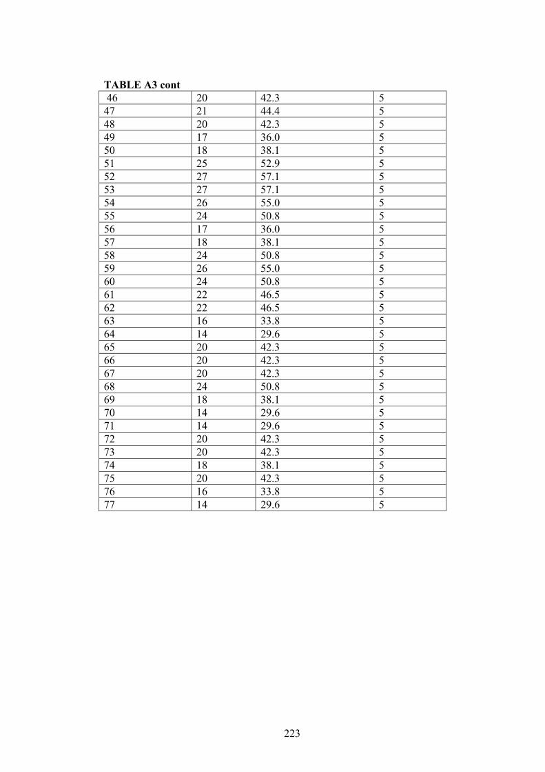
223
TABLE A3 cont 46 20 42.3 5 47 21 44.4 5 48 20 42.3 5 49 17 36.0 5 50 18 38.1 5 51 25 52.9 5 52 27 57.1 5 53 27 57.1 5 54 26 55.0 5 55 24 50.8 5 56 17 36.0 5 57 18 38.1 5 58 24 50.8 5 59 26 55.0 5 60 24 50.8 5 61 22 46.5 5 62 22 46.5 5 63 16 33.8 5 64 14 29.6 5 65 20 42.3 5 66 20 42.3 5 67 20 42.3 5 68 24 50.8 5 69 18 38.1 5 70 14 29.6 5 71 14 29.6 5 72 20 42.3 5 73 20 42.3 5 74 18 38.1 5 75 20 42.3 5 76 16 33.8 5 77 14 29.6 5

224
TABLE A4 Intensity data for Speed setting 3 and a delay of 1s Cup no: Volume
[mL] Measured intensity [mm/hr]
Duration [min]
1 46 97.3 5 2 52 110.0 5 3 50 105.7 5 4 50 105.7 5 5 45 95.2 5 6 44 93.0 5 7 32 67.7 5 8 55 116.3 5 9 66 139.6 5 10 68 143.8 5 11 66 139.6 5 12 68 143.8 5 13 62 131.1 5 14 40 84.6 5 15 69 145.9 5 16 76 160.7 5 17 74 156.5 5 18 72 152.3 5 19 70 148.0 5 20 64 135.3 5 21 44 93.0 5 22 62 131.1 5 23 80 169.2 5 24 80 169.2 5 25 80 169.2 5 26 76 160.7 5 27 66 139.6 5 28 44 93.0 5 29 56 118.4 5 30 70 148.0 5 31 74 156.5 5 32 70 148.0 5 33 66 139.6 5 34 58 122.7 5 35 42 88.8 5 36 54 114.2 5 37 68 143.8 5 38 82 173.4 5 39 76 160.7 5 40 77 162.8 5 41 78 164.9 5 42 73 154.4 5 43 54 114.2 5 44 62 131.1 5 45 66 139.6 5

225
TABLE A4 cont 46 68 143.8 5 47 64 135.3 5 48 60 126.9 5 49 46 97.3 5 50 60 126.9 5 51 78 164.9 5 52 80 169.2 5 53 80 169.2 5 54 80 169.2 5 55 72 152.3 5 56 52 110.0 5 57 58 122.7 5 58 76 160.7 5 59 80 169.2 5 60 76 160.7 5 61 72 152.3 5 62 56 118.4 5 63 52 110.0 5 64 50 105.7 5 65 64 135.3 5 66 66 139.6 5 67 63 133.2 5 68 76 160.7 5 69 58 122.7 5 70 48 101.5 5 71 44 93.0 5 72 54 114.2 5 73 61 129.0 5 74 58 122.7 5 75 70 148.0 5 76 48 101.5 5 77 41 86.7 5

226
TABLE A5 Intensity data for Speed setting 3 and a delay of 1.5s Cup no: Volume
[mL] Measured intensity [mm/hr]
Duration [min]
1 32 67.7 5 2 44 93.0 5 3 43 90.9 5 4 45 95.2 5 5 40 84.6 5 6 38 80.4 5 7 31 65.6 5 8 36 76.1 5 9 58 122.7 5 10 70 148.0 5 11 64 135.3 5 12 65 137.5 5 13 60 126.9 5 14 50 105.7 5 15 40 84.6 5 16 66 139.6 5 17 72 152.3 5 18 68 143.8 5 19 65 137.5 5 20 61 129.0 5 21 49 103.6 5 22 44 93.0 5 23 66 139.6 5 24 71 150.1 5 25 72 152.3 5 26 67 141.7 5 27 61 129.0 5 28 46 97.3 5 29 42 88.8 5 30 60 126.9 5 31 63 133.2 5 32 63 133.2 5 33 58 122.7 5 34 56 118.4 5 35 42 88.8 5 36 70 148.0 5 37 72 152.3 5 38 72 152.3 5 39 68 143.8 5 40 68 143.8 5 41 61 129.0 5 42 58 122.7 5 43 48 101.5 5 44 57 120.5 5 45 60 126.9 5

227
TABLE A5 cont 46 59 124.8 5 47 54 114.2 5 48 50 105.7 5 49 40 84.6 5 50 53 112.1 5 51 61 129.0 5 52 72 152.3 5 53 72 152.3 5 54 68 143.8 5 55 62 131.1 5 56 45 95.2 5 57 52 110.0 5 58 68 143.8 5 59 70 148.0 5 60 66 139.6 5 61 65 137.5 5 62 60 126.9 5 63 43 90.9 5 64 46 97.3 5 65 60 126.9 5 66 65 137.5 5 67 58 122.7 5 68 59 124.8 5 69 52 110.0 5 70 40 84.6 5 71 48 101.5 5 72 52 110.0 5 73 51 107.9 5 74 50 105.7 5 75 50 105.7 5 76 50 105.7 5 77 38 80.4 5

228
TABLE A6 Intensity data for Speed setting 3 and a delay of 5s Cup no: Volume
[mL] Measured intensity [mm/hr]
Duration [min]
1 17 36.0 5 2 17 36.0 5 3 20 42.3 5 4 20 42.3 5 5 19 40.2 5 6 18 38.1 5 7 13 27.5 5 8 24 50.8 5 9 28 59.2 5 10 27 57.1 5 11 27 57.1 5 12 28 59.2 5 13 26 55.0 5 14 15 31.7 5 15 24 50.8 5 16 30 63.4 5 17 30 63.4 5 18 30 63.4 5 19 29 61.3 5 20 27 57.1 5 21 18 38.1 5 22 25 52.9 5 23 33 69.8 5 24 33 69.8 5 25 31 65.6 5 26 30 63.4 5 27 29 61.3 5 28 18 38.1 5 29 23 48.6 5 30 29 61.3 5 31 29 61.3 5 32 29 61.3 5 33 28 59.2 5 34 23 48.6 5 35 16 33.8 5 36 21 44.4 5 37 27 57.1 5 38 35 74.0 5 39 31 65.6 5 40 31 65.6 5 41 32 67.7 5 42 27 57.1 5 43 28 59.2 5 44 26 55.0 5 45 27 57.1 5

229
TABLE A6 cont 46 27 57.1 5 47 25 52.9 5 48 24 50.8 5 49 19 40.2 5 50 25 52.9 5 51 36 76.1 5 52 33 69.8 5 53 33 69.8 5 54 32 67.7 5 55 39 82.5 5 56 21 44.4 5 57 24 50.8 5 58 32 67.7 5 59 32 67.7 5 60 31 65.6 5 61 32 67.7 5 62 27 57.1 5 63 20 42.3 5 64 19 40.2 5 65 25 52.9 5 66 27 57.1 5 67 26 55.0 5 68 30 63.4 5 69 23 48.6 5 70 18 38.1 5 71 19 40.2 5 72 27 57.1 5 73 26 55.0 5 74 24 50.8 5 75 22 46.5 5 76 20 42.3 5 77 19 40.2 5

230
TABLE A7 Calibration of median drop size using flour pellet method
Sieve No. of pellets Total Mass of pellets [mg]
Average pellet mass [mg]
Drop mass according to Hudson (1963) [mg]
4.75 mm 9 382.4 42.49 54.17 3.35 mm 74 1443.9 19.51 24.88 2.36 mm 125 1286 10.29 12.86 1.18 mm 807 2058.4 2.55 2.86 0.6 mm 3200 504.3 0.16 0.11 0.5 mm 3389 463.2 0.14 0.09
Sieve Average drop volume
[cm3] Average drop diameter
[cm] Total Volume [cm3] % of total volume
4.75 mm 0.054 0.47 0.49 7.08 3.35 mm 0.025 0.36 1.84 26.74 2.36 mm 0.013 0.29 1.61 23.35 1.18 mm 0.0029 0.18 2.31 33.48 0.6 mm 0.00011 0.058 0.34 4.91 0.5 mm 0.000090 0.056 0.31 4.44
Drop diameter [mm] % of total volume % Cumulative
volume 0 0.55 4.44 4.44 0.59 4.91 9.35 1.76 33.48 42.83 2.91 23.35 66.18 3.62 26.74 92.92 4.69 7.08 100

231
TABLE A8 Rainfall quality analyses in Brisbane Station Date collected Date
measured pH EC
(μS/cm) DOC (mg/L)
Camp Hill 11/03/2003 8am 13/03/2003 5.40 26.30 5.381
Camp Hill 13/2 2003 14/2 2003 5.90 33.30 na
QUT 19/2 2003 11am 19/2 2003 6.75 228.00 na
QUT 19/2 2003 4pm 19/2 2003 6.10 76.30 14.71
QUT 11/03/2003 11am 13/03/2003 7.20 69.20 na
QUT 13/03/03 9.00 am 13/03/2003 6.80 53.30 7.354
Toowong 19/2 2003 7pm 20/2 2003 6.15 19.00 8.713
Camp Hill 19/2 2003 8pm 20/2 2003 6.20 19.70 5.629
Toowong 21/2 2003 7am 21/2 2003 7.10 92.70 11.07
Toowong 12/03/2003 7pm 13/03/2003 5.90 33.20 6.505
QUT 21/2 2003 8am 21/2 2003 6.80 85.50 11.98
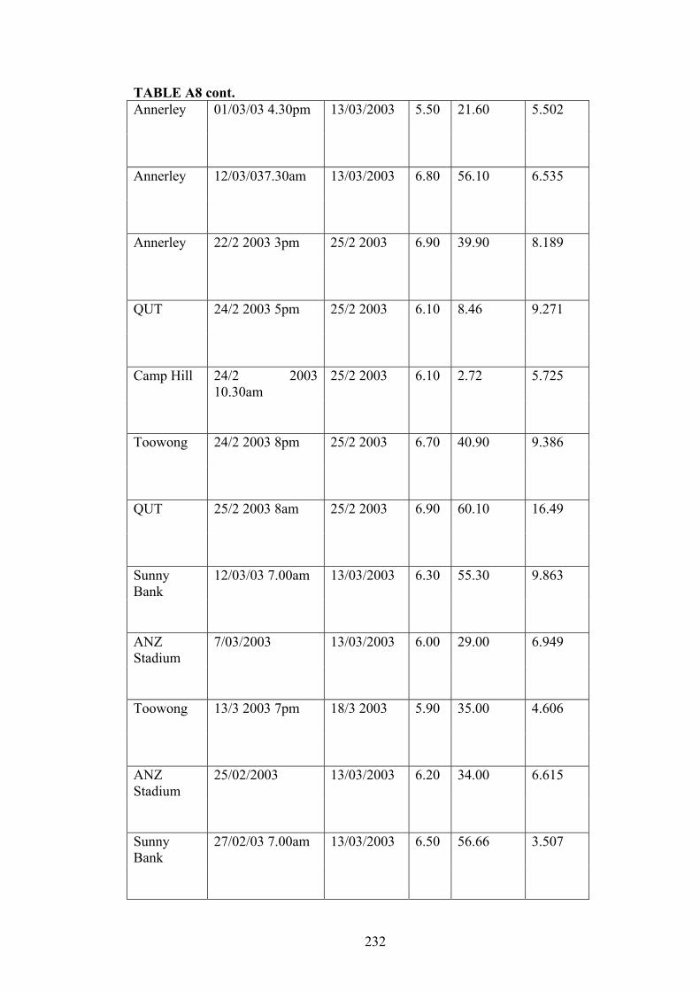
232
TABLE A8 cont. Annerley 01/03/03 4.30pm 13/03/2003 5.50 21.60 5.502
Annerley 12/03/037.30am 13/03/2003 6.80 56.10 6.535
Annerley 22/2 2003 3pm 25/2 2003 6.90 39.90 8.189
QUT 24/2 2003 5pm 25/2 2003 6.10 8.46 9.271
Camp Hill 24/2 2003 10.30am
25/2 2003 6.10 2.72 5.725
Toowong 24/2 2003 8pm 25/2 2003 6.70 40.90 9.386
QUT 25/2 2003 8am 25/2 2003 6.90 60.10 16.49
Sunny Bank
12/03/03 7.00am 13/03/2003 6.30 55.30 9.863
ANZ Stadium
7/03/2003 13/03/2003 6.00 29.00 6.949
Toowong 13/3 2003 7pm 18/3 2003 5.90 35.00 4.606
ANZ Stadium
25/02/2003 13/03/2003 6.20 34.00 6.615
Sunny Bank
27/02/03 7.00am 13/03/2003 6.50 56.66 3.507

233
FIGURE A1 Delonghi Aqualand Vacuum cleaner specification

234

235
APPENDIX B
TEST RESULTS

236
TABLE B1 – Residential wash-off data PART 2 (Data for simulated rainfall events with intensities 86 and 115mm/hr)
1y10m >300 20/08/2003 86 10 EMC 1 year 10 min 42 0.03 0.27 2 7.601y10m 151-300 20/08/2003 86 10 EMC 1 year 10 min 42 0.03 0.27 2 7.60 1y10m 76-150 20/08/2003 86 10 EMC 1 year 10 min 42 0.03 0.27 2 7.60 1y10m 0.45-75 20/08/2003 86 10 EMC 1 year 10 min 42 0.03 0.27 2 7.60 1y10min Dis 20/08/2003 86 10 EMC 1 year 10 min 42 0.03 0.27 2 7.602y20m >300 20/08/2003 86 20 EMC 2 year 20 min 84 0.03 0.27 2 7.60
2y20m 151-300 20/08/2003 86 20 EMC 2 year 20 min 84 0.03 0.27 2 7.602y20m 76-150 20/08/2003 86 20 EMC 2 year 20 min 84 0.03 0.27 2 7.602y20m 0.45-75 20/08/2003 86 20 EMC 2 year 20 min 84 0.03 0.27 2 7.602y20min Dis 20/08/2003 86 20 EMC 2 year 20 min 84 0.03 0.27 2 7.6010y40m >300 20/08/2003 86 40 EMC 10 year 40 min 167 0.03 0.27 2 7.60
10y40m 151-300 20/08/2003 86 40 EMC 10 year 40 min 167 0.03 0.27 2 7.6010y40m 76-150 20/08/2003 86 40 EMC 10 year 40 min 167 0.03 0.27 2 7.6010y40m 0.45-75 20/08/2003 86 40 EMC 10 year 40 min 167 0.03 0.27 2 7.6010y40min Dis 20/08/2003 86 40 EMC 10 year 40 min 167 0.03 0.27 2 7.60
1y5m >300 20/08/2003 115 5 EMC 1 year 5 min 22 0.03 0.27 2 7.601y5m 151-300 20/08/2003 115 5 EMC 1 year 5 min 22 0.03 0.27 2 7.601y5m 76-150 20/08/2003 115 5 EMC 1 year 5 min 22 0.03 0.27 2 7.601y5m 0.45-75 20/08/2003 115 5 EMC 1 year 5 min 22 0.03 0.27 2 7.601y5min Dis 20/08/2003 115 5 EMC 1 year 5 min 22 0.03 0.27 2 7.60
Dry days b f
Last rainfall[mm]
Event Total volume [L]
Slope [m/m]
Texture depth [mm]
Sample name [ARI andparticle size (µm)]
Sample date
Intensity [mm/hr]
Duration [min]

237
TABLE B1 – Residential wash-off data PART 1 (Parameters continued from previous page)
1y10m >300 39 18.4 6.99 124.90 0.457 1.127 0.951y10m 151-300 39 8.38 6.99 124.90 1.199 0.709 1.501y10m 76-150 39 18.65 6.99 124.90 0.827 0.387 5.301y10m 0.45-75 39 53.09 6.99 124.90 1.583 0.003 16.451y10min Dis 39 1.48 6.99 124.90 9.447 3.603 95.00 2y20m >300 39 6.41 7.20 127.60 0.193 2.779 1.05
2y20m 151-300 39 22.17 7.20 127.60 2.041 0.132 2.102y20m 76-150 39 18.39 7.20 127.60 0.225 0.186 9.10
2y20m 0.45-75 39 51.45 7.20 127.60 1.081 0.478 16.702y20min Dis 39 1.58 7.20 127.60 8.009 3.311 75.0010y40m >300 39 10.63 7.30 130.00 0.250 2.935 0.67
10y40m 151-300 39 32.92 7.30 130.00 1.859 0.665 0.8310y40m 76-150 39 28.83 7.30 130.00 0.006 0.688 4.0010y40m 0.45-75 39 27.62 7.30 130.00 0.265 1.989 7.6010y40min Dis 39 <0.01 7.30 130.00 6.412 3.608 80.00
1y5m >300 39 3.79 6.81 122.00 3.701 1.914 3.401y5m 151-300 39 12.18 6.81 122.00 0.509 0.635 19.40 1y5m 76-150 39 17.73 6.81 122.00 4.033 1.282 27.101y5m 0.45-75 39 64.52 6.81 122.00 2.218 0.038 76.301y5min Dis 39 1.78 6.81 122.00 9.402 1.118 70.00
2417.33
2186.39
2789.02
Total solids [mg]
1004.30
Sample name [ARI andparticle size (µm)]
Last swept[days]
Particle volumepercentage [%]
TSS [mg/L]
pH EC [uS/cm]
TOC [ppm]
IC [ppm]
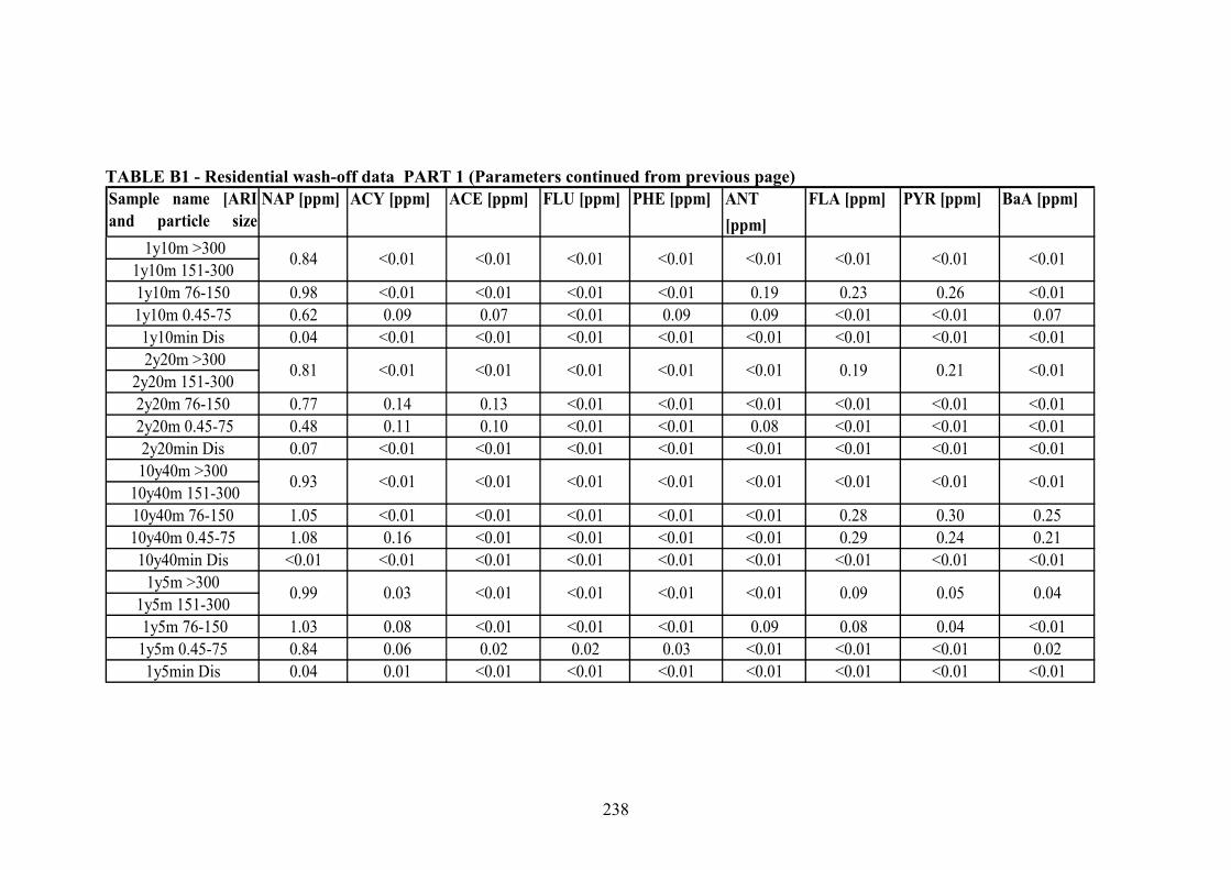
238
TABLE B1 - Residential wash-off data PART 1 (Parameters continued from previous page)
1y10m >3001y10m 151-3001y10m 76-150 0.98 <0.01 <0.01 <0.01 <0.01 0.19 0.23 0.26 <0.011y10m 0.45-75 0.62 0.09 0.07 <0.01 0.09 0.09 <0.01 <0.01 0.071y10min Dis 0.04 <0.01 <0.01 <0.01 <0.01 <0.01 <0.01 <0.01 <0.01 2y20m >300
2y20m 151-3002y20m 76-150 0.77 0.14 0.13 <0.01 <0.01 <0.01 <0.01 <0.01 <0.01 2y20m 0.45-75 0.48 0.11 0.10 <0.01 <0.01 0.08 <0.01 <0.01 <0.01
2y20min Dis 0.07 <0.01 <0.01 <0.01 <0.01 <0.01 <0.01 <0.01 <0.0110y40m >300
10y40m 151-30010y40m 76-150 1.05 <0.01 <0.01 <0.01 <0.01 <0.01 0.28 0.30 0.2510y40m 0.45-75 1.08 0.16 <0.01 <0.01 <0.01 <0.01 0.29 0.24 0.2110y40min Dis <0.01 <0.01 <0.01 <0.01 <0.01 <0.01 <0.01 <0.01 <0.01
1y5m >3001y5m 151-300 1y5m 76-150 1.03 0.08 <0.01 <0.01 <0.01 0.09 0.08 0.04 <0.011y5m 0.45-75 0.84 0.06 0.02 0.02 0.03 <0.01 <0.01 <0.01 0.021y5min Dis 0.04 0.01 <0.01 <0.01 <0.01 <0.01 <0.01 <0.01 <0.01
Sample name [ARIand particle size( )
NAP [ppm] ACY [ppm] ACE [ppm] FLU [ppm] PHE [ppm] ANT [ppm]
FLA [ppm] PYR [ppm] BaA [ppm]
0.84 <0.01 <0.01 <0.01 <0.01 <0.01 <0.01 <0.01 <0.01
0.81 <0.01 <0.01 <0.01 <0.01 <0.01 0.19 0.21 <0.01
0.93 <0.01 <0.01 <0.01 <0.01 <0.01 <0.01 <0.01 <0.01
0.99 0.03 <0.01 <0.01 0.04<0.01 <0.01 0.09 0.05

239
TABLE B1 – Residential wash-off data PART 1 (Parameters continued from previous page)
1y10m >300 0.4801y10m 151-300 0.4001y10m 76-150 <0.01 <0.01 <0.01 <0.01 <0.01 <0.01 0.5601y10m 0.45-75 <0.01 0.128 <0.01 <0.01 <0.01 <0.01 0.6001y10min Dis <0.01 <0.01 <0.01 <0.01 <0.01 <0.01 0.014 2y20m >300 0.108
2y20m 151-300 0.1842y20m 76-150 <0.01 <0.01 <0.01 <0.01 <0.01 <0.01 0.288
2y20m 0.45-75 <0.01 <0.01 0.060 <0.01 <0.01 <0.01 0.1162y20min Dis <0.01 <0.01 <0.01 <0.01 <0.01 <0.01 <0.00510y40m >300 0.344
10y40m 151-300 0.19610y40m 76-150 <0.01 <0.01 0.250 <0.01 <0.01 <0.01 0.27210y40m 0.45-75 <0.01 <0.01 0.224 <0.01 <0.01 <0.01 0.13210y40min Dis <0.01 <0.01 0.011 <0.01 <0.01 <0.01 <0.005
1y5m >300 0.1001y5m 151-300 0.172 1y5m 76-150 <0.01 <0.01 <0.01 <0.01 <0.01 <0.01 0.4401y5m 0.45-75 <0.01 <0.01 <0.01 <0.01 <0.01 <0.01 0.7201y5min Dis <0.01 <0.01 <0.01 <0.01 <0.01 <0.01 0.026
Sample name [ARI andparticle size (µm)]
CHR [ppm]
BbF [ppm] BaP [ppm] IND [ppm] DbA [ppm] BgP [ppm] Fe [ppm]
<0.01 <0.01 <0.01 <0.01 <0.01 <0.01
<0.01 <0.01
<0.01 <0.01
<0.01 <0.01
<0.01 <0.01 <0.01 <0.01
<0.01 <0.01
<0.01 <0.01<0.01 <0.01 <0.01 <0.01
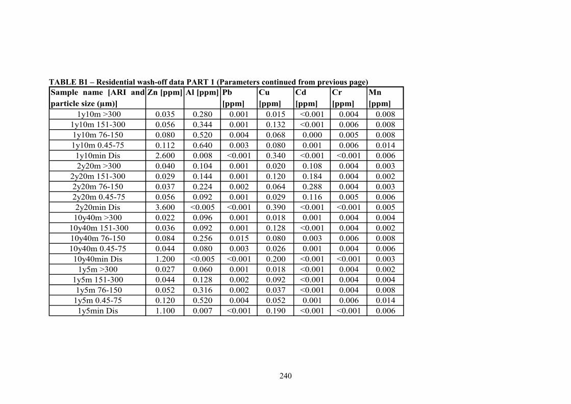
240
TABLE B1 – Residential wash-off data PART 1 (Parameters continued from previous page)
1y10m >300 0.035 0.280 0.001 0.015 <0.001 0.004 0.0081y10m 151-300 0.056 0.344 0.001 0.132 <0.001 0.006 0.0081y10m 76-150 0.080 0.520 0.004 0.068 0.000 0.005 0.0081y10m 0.45-75 0.112 0.640 0.003 0.080 0.001 0.006 0.0141y10min Dis 2.600 0.008 <0.001 0.340 <0.001 <0.001 0.006 2y20m >300 0.040 0.104 0.001 0.020 0.108 0.004 0.003
2y20m 151-300 0.029 0.144 0.001 0.120 0.184 0.004 0.0022y20m 76-150 0.037 0.224 0.002 0.064 0.288 0.004 0.003
2y20m 0.45-75 0.056 0.092 0.001 0.029 0.116 0.005 0.0062y20min Dis 3.600 <0.005 <0.001 0.390 <0.001 <0.001 0.00510y40m >300 0.022 0.096 0.001 0.018 0.001 0.004 0.004
10y40m 151-300 0.036 0.092 0.001 0.128 <0.001 0.004 0.00210y40m 76-150 0.084 0.256 0.015 0.080 0.003 0.006 0.00810y40m 0.45-75 0.044 0.080 0.003 0.026 0.001 0.004 0.00610y40min Dis 1.200 <0.005 <0.001 0.200 <0.001 <0.001 0.003
1y5m >300 0.027 0.060 0.001 0.018 <0.001 0.004 0.0021y5m 151-300 0.044 0.128 0.002 0.092 <0.001 0.004 0.004 1y5m 76-150 0.052 0.316 0.002 0.037 <0.001 0.004 0.0081y5m 0.45-75 0.120 0.520 0.004 0.052 0.001 0.006 0.0141y5min Dis 1.100 0.007 <0.001 0.190 <0.001 <0.001 0.006
Cu [ppm]
Cd [ppm]
Cr [ppm]
Mn [ppm]
Sample name [ARI andparticle size (µm)]
Zn [ppm] Al [ppm] Pb [ppm]

241
TABLE B1 – Residential Wash-off data PART 2 (Data for simulated rainfall events with intensities 115 and 133mm/hr)
2y10m >300 20/08/2003 115 10 EMC 2 year 10 min 42 0.03 0.27 2 7.60 2y10m 151-300 20/08/2003 115 10 EMC 2 year 10 min 42 0.03 0.27 2 7.60 2y10m 76-150 20/08/2003 115 10 EMC 2 year 10 min 42 0.03 0.27 2 7.60 2y10m 0.45-75 20/08/2003 115 10 EMC 2 year 10 min 42 0.03 0.27 2 7.60 2y10min Dis 20/08/2003 115 10 EMC 2 year 10 min 42 0.03 0.27 2 7.60 10y25m >300 20/08/2003 115 25 EMC 10 year 25 min 134 0.03 0.27 2 7.60
10y25m 151-300 20/08/2003 115 25 EMC 10 year 25 min 134 0.03 0.27 2 7.60 10y25m 76-150 20/08/2003 115 25 EMC 10 year 25 min 134 0.03 0.27 2 7.60 10y25m 0.45-75 20/08/2003 115 25 EMC 10 year 25 min 134 0.03 0.27 2 7.60
10y25min Dis 20/08/2003 115 25 EMC 10 year 25 min 134 0.03 0.27 2 7.60 2y7m >300 20/08/2003 133 7 EMC 2 year 7 min 28 0.02 0.27 2 7.60
2y7m 151-300 20/08/2003 133 7 EMC 2 year 7 min 28 0.02 0.27 2 7.60 2y7m 76-150 20/08/2003 133 7 EMC 2 year 7 min 28 0.02 0.27 2 7.60 2y7m 0.45-75 20/08/2003 133 7 EMC 2 year 7 min 28 0.02 0.27 2 7.60 2y7min Dis 20/08/2003 133 7 EMC 2 year 7 min 28 0.02 0.27 2 7.60 5y13m >300 20/08/2003 133 13 EMC 5 year 13 min 54 0.02 0.27 2 7.60
5y13m 151-300 20/08/2003 133 13 EMC 5 year 13 min 54 0.02 0.27 2 7.60 5y13m 76-150 20/08/2003 133 13 EMC 5 year 13 min 54 0.02 0.27 2 7.60 5y13m 0.45-75 20/08/2003 133 13 EMC 5 year 13 min 54 0.02 0.27 2 7.60 5y13min Dis 20/08/2003 133 13 EMC 5 year 13 min 54 0.02 0.27 2 7.60 10y17m >300 20/08/2003 133 17 EMC 10 year 17 min 85 0.02 0.27 2 7.60
10y17m 151-300 20/08/2003 133 17 EMC 10 year 17 min 85 0.02 0.27 2 7.60 10y17m 76-150 20/08/2003 133 17 EMC 10 year 17 min 85 0.02 0.27 2 7.60 10y17m 0.45-75 20/08/2003 133 17 EMC 10 year 17 min 85 0.02 0.27 2 7.60 10y17min Dis 20/08/2003 133 17 EMC 10 year 17 min 85 0.02 0.27 2 7.60
Sample name [ARI andparticle size (µm)]
Sample date Intensity [mm/hr]
Duration [min]
Dry daysbefore
Last rainfall
Event Total volumeevent [L]
Slope [m/m]
Texture depth

242
TABLE B1 - Residential wash-off data PART 2 (Parameters continued from previous page)
2y10m >300 39 0.13 6.93 118.60 1.708 1.246 0.51 2y10m 151-300 39 6.63 6.93 118.60 2.538 0.400 1.71 2y10m 76-150 39 21.43 6.93 118.60 1.714 0.754 11.84 1.01 0.13 2y10m 0.45-75 39 70.56 6.93 118.60 1.093 0.217 34.62 1.01 0.06 2y10min Dis 39 1.25 6.93 118.60 8.398 2.212 65.00 0.07 <0.01 10y25m >300 39 0.01 7.00 112.80 0.627 2.909 0.95
10y25m 151-300 39 10.13 7.00 112.80 1.276 0.236 0.80 10y25m 76-150 39 32.91 7.00 112.80 0.222 0.174 3.55 0.99 <0.01 10y25m 0.45-75 39 55.97 7.00 112.80 1.826 2.489 16.20 1.23 0.13
10y25min Dis 39 0.89 7.00 112.80 6.369 3.270 60.00 0.06 <0.01 2y7m >300 39 0.13 6.65 104.40 0.419 3.042 2.40
2y7m 151-300 39 2.65 6.65 104.40 0.648 0.582 5.30 2y7m 76-150 39 13.06 6.65 104.40 1.489 0.712 8.90 1.15 <0.01 2y7m 0.45-75 39 82.8 6.65 104.40 0.528 0.578 48.20 0.95 0.18 2y7min Dis 39 1.36 6.65 104.40 6.886 3.214 90.00 0.05 0.01
5y13m >300 39 2.8 6.87 102.00 1.280 2.884 1.01 5y13m 151-300 39 7.16 6.87 102.00 1.135 0.830 1.14 5y13m 76-150 39 17.43 6.87 102.00 0.072 0.493 2.78 1.01 0.11 5y13m 0.45-75 39 71.43 6.87 102.00 0.083 0.443 26.71 1.12 0.11 5y13min Dis 39 1.18 6.87 102.00 5.973 3.127 80.00 0.03 <0.01 10y17m >300 39 2.09 7.06 105.10 0.835 1.824 0.86
10y17m 151-300 39 9.82 7.06 105.10 1.344 0.559 0.86 10y17m 76-150 39 18.78 7.06 105.10 0.029 0.290 3.29 1.06 0.15 10y17m 0.45-75 39 68.19 7.06 105.10 0.498 0.397 20.79 1.11 0.19 10y17min Dis 39 1.12 7.06 105.10 6.164 3.336 85.00 0.04 <0.01
1711.72
0.98 <0.01
2190.42
0.84 <0.01
2870.25
0.89 0.17
1833.84
1.10 0.14
TSS [mg/L]
NAP [ppm]
ACY [ppm]
2039.69
0.97 <0.01
EC [uS/cm]
TOC [ppm]
IC [ppm] Total solids [mg]Sample name [ARI andparticle size (µm)]
Last swept[days]
Particle volumepercentage [%]
pH
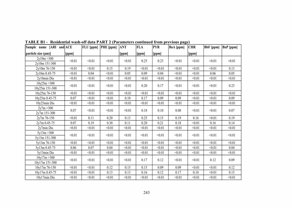
243
TABLE B1 - Residential wash-off data PART 2 (Parameters continued from previous page)
2y10m >300 2y10m 151-300 2y10m 76-150 <0.01 <0.01 0.15 0.19 <0.01 <0.01 <0.01 <0.01 <0.01 0.13 2y10m 0.45-75 <0.01 0.04 <0.01 0.05 0.09 0.04 <0.01 <0.01 0.06 0.05 2y10min Dis <0.01 <0.01 <0.01 <0.01 <0.01 <0.01 <0.01 <0.01 <0.01 <0.01 10y25m >300
10y25m 151-300 10y25m 76-150 <0.01 <0.01 <0.01 <0.01 <0.01 <0.01 <0.01 <0.01 <0.01 <0.01 10y25m 0.45-75 0.07 <0.01 <0.01 0.10 0.17 0.09 0.09 <0.01 <0.01 0.09
10y25min Dis <0.01 <0.01 <0.01 <0.01 <0.01 <0.01 <0.01 <0.01 <0.01 <0.01 2y7m >300
2y7m 151-300 2y7m 76-150 <0.01 0.11 0.20 0.13 0.25 0.15 0.19 0.16 <0.01 0.19 2y7m 0.45-75 0.07 0.19 0.30 0.11 0.20 0.21 0.18 <0.01 0.16 0.14 2y7min Dis <0.01 <0.01 <0.01 <0.01 <0.01 <0.01 <0.01 <0.01 <0.01 <0.01 5y13m >300
5y13m 151-300 5y13m 76-150 <0.01 <0.01 <0.01 <0.01 <0.01 <0.01 <0.01 <0.01 <0.01 <0.01 5y13m 0.45-75 0.06 0.07 0.04 <0.01 <0.01 <0.01 <0.01 <0.01 <0.01 0.04 5y13min Dis <0.01 <0.01 <0.01 <0.01 <0.01 <0.01 <0.01 <0.01 <0.01 <0.01 10y17m >300
10y17m 151-300 10y17m 76-150 <0.01 <0.01 0.12 0.15 0.15 0.09 0.09 <0.01 <0.01 0.12 10y17m 0.45-75 <0.01 <0.01 0.13 0.13 0.16 0.12 0.17 0.10 <0.01 0.15 10y17min Dis <0.01 <0.01 <0.01 <0.01 <0.01 <0.01 <0.01 <0.01 <0.01 <0.01
0.12 0.090.17 0.12 <0.01 <0.01<0.01 <0.01 <0.01 <0.01
<0.01 <0.01 <0.01
<0.01 0.07
<0.01 <0.01 <0.01 <0.01 <0.01 <0.01 <0.01
0.18 0.10 0.08 <0.010.07 <0.01 <0.01 <0.01
<0.01 <0.01 0.23
<0.01 <0.01
<0.01 <0.01 <0.01 <0.01 0.20 0.17 <0.01
0.25 0.23 <0.01 <0.01<0.01 <0.01 <0.01 <0.01
CHR [ppm]
BbF [ppm] BaP [ppm]ANT [ppm]
FLA [ppm]
PYR [ppm]
BaA [ppm]Sample name [ARI andparticle size (µm)]
ACE [ppm]
FLU [ppm] PHE [ppm]

244
TABLE B1 - Residential wash-off data PART 2 (Parameters continued from previous page)
2y10m >300 0.144 0.056 0.152 0.004 0.021 0.001 0.006 0.003 2y10m 151-300 0.248 0.048 0.160 0.001 0.148 0.001 0.006 0.004 2y10m 76-150 <0.01 <0.01 <0.01 0.336 0.040 0.252 0.002 0.030 0.001 0.004 0.005 2y10m 0.45-75 <0.01 <0.01 <0.01 0.480 0.084 0.372 0.003 0.044 0.001 0.006 0.010 2y10min Dis <0.01 <0.01 <0.01 0.008 1.100 0.005 <0.001 0.160 <0.001 <0.001 0.004 10y25m >300 0.088 0.033 0.064 0.001 0.022 0.001 0.004 0.002
10y25m 151-300 0.152 0.026 0.100 0.001 0.164 <0.001 0.003 0.004 10y25m 76-150 <0.01 <0.01 <0.01 0.196 0.038 0.156 0.002 0.027 <0.001 0.002 0.004 10y25m 0.45-75 <0.01 <0.01 <0.01 0.104 0.035 0.088 0.001 0.025 <0.001 0.002 0.004
10y25min Dis <0.01 <0.01 <0.01 <0.005 0.970 <0.005 <0.001 0.170 <0.001 <0.001 0.002 2y7m >300 0.068 0.023 0.048 <0.001 0.016 <0.001 0.007 0.002
2y7m 151-300 0.108 0.044 0.072 <0.001 0.168 <0.001 0.004 0.002 2y7m 76-150 <0.01 <0.01 <0.01 0.140 0.036 0.084 0.001 0.056 <0.001 0.004 0.003 2y7m 0.45-75 <0.01 <0.01 <0.01 0.560 0.076 0.364 0.002 0.039 <0.001 0.003 0.010 2y7min Dis <0.01 <0.01 <0.01 <0.005 0.800 <0.005 <0.001 0.140 <0.001 <0.001 0.003 5y13m >300 0.096 0.028 0.052 <0.001 0.010 <0.001 0.001 0.002
5y13m 151-300 0.108 0.036 0.120 0.003 0.064 <0.001 0.002 0.002 5y13m 76-150 <0.01 <0.01 <0.01 0.148 0.052 0.124 0.001 0.016 <0.001 0.005 0.002 5y13m 0.45-75 <0.01 <0.01 <0.01 0.392 0.060 0.364 0.002 0.032 <0.001 0.002 0.008 5y13min Dis <0.01 <0.01 <0.01 <0.005 0.610 0.006 <0.001 0.110 <0.001 <0.001 0.004 10y17m >300 0.037 0.040 0.040 <0.001 0.014 <0.001 0.002 0.001
10y17m 151-300 0.076 0.040 0.048 <0.001 0.048 <0.001 0.004 0.001 10y17m 76-150 <0.01 <0.01 <0.01 0.076 0.030 0.064 0.001 0.016 <0.001 0.004 0.002 10y17m 0.45-75 <0.01 <0.01 <0.01 0.124 0.040 0.080 0.001 0.018 <0.001 0.005 0.004 10y17min Dis <0.01 <0.01 <0.01 <0.005 0.620 <0.005 <0.001 0.120 <0.001 <0.001 0.005
<0.01 <0.01
<0.01
<0.01
<0.01
<0.01
<0.01
<0.01 <0.01
<0.01 <0.01
<0.01 <0.01
<0.01 <0.01
Cu [ppm]
Cd [ppm]
Cr [ppm]
Mn [ppm]
Fe [ppm] Zn [ppm] Al [ppm] Pb [ppm]
Sample name [ARI andparticle size (µm)]
IND [ppm]
DbA [ppm] BgP [ppm]

245
TABLE B1 – Residential Wash-off data PART 3 (Blanks and replicate samples)
Field blank 20/08/2003 115 BLANKField blank 20/08/2003 115 BLANKField blank 20/08/2003 86 BLANKField blank 20/08/2003 86 BLANKField blank 20/08/2003 133 BLANKField blank 20/08/2003 133 BLANK
Laboratory blank 20/08/2003 - Distilled blankLaboratory blank 20/08/2003 - Distilled blank
Build-up <0.45 Rep 20/08/2003 - Replicate10y25min Dis Rep 20/08/2003 115 115 Replicate
Build-up 76-150 Rep 20/08/2003 - Replicate2y7 0.45-75 Rep 20/08/2003 133 133 Replicate
Sample name Sample date Intensity [mm/hr]
Duration [min]
Dry daysbefore
Last rainfall [ ]
Event Total volumeevent [L]
Slope [m/m]
Texture depth [ ]
Field blank 7.07 99.70 6.367 4.013 <0.01 <0.01 <0.01Field blank 7.07 99.70 <0.001 <0.001 0.02 0.04 <0.01Field blank 7.15 119.70 5.256 4.335 <0.01 <0.01 <0.01Field blank 7.15 119.70 <0.001 <0.001 0.01 0.04 <0.01Field blank 7.02 97.60 5.689 2.972 <0.01 <0.01 <0.01Field blank 7.02 97.60 <0.001 <0.001 0.04 0.05 <0.01
Laboratory blank 6.27 8.76 4.124 <0.001 <0.01 <0.01 <0.01Laboratory blank 6.27 8.76 <0.001 <0.001 <0.01 0.02 <0.01
Build-up <0.45 Rep - - 4.135 1.844 35.00 0.08 0.0210y25min Dis Rep - - 6.298 3.274 60.00 0.07 <0.01
Build-up 76-150 Rep - - 4.125 0.000 96.15 1.24 0.162y7 0.45-75 Rep - - 0.519 0.598 47.90 0.95 0.18
EC [uS/cm]
NAP [ppm]Sample name ACY [ppm]TOC [ppm]
IC [ppm]
TSS [mg/L]
Last swept [d ]
Particle volumepercentage [%]
pH

246
TABLE B1 – Residential Wash-off data PART 3 (Parameters continued from previous page)
Field blank <0.01 <0.01 <0.01 <0.01 <0.01 <0.01 <0.01 <0.01 <0.01Field blank <0.01 <0.01 <0.01 <0.01 <0.01 <0.01 <0.01 <0.01 <0.01Field blank <0.01 <0.01 <0.01 <0.01 <0.01 <0.01 <0.01 <0.01 <0.01Field blank <0.01 <0.01 <0.01 <0.01 <0.01 <0.01 <0.01 <0.01 <0.01Field blank <0.01 <0.01 <0.01 <0.01 <0.01 <0.01 <0.01 <0.01 <0.01Field blank <0.01 <0.01 <0.01 <0.01 <0.01 <0.01 <0.01 <0.01 <0.01
Laboratory blank <0.01 <0.01 <0.01 <0.01 <0.01 <0.01 <0.01 <0.01 <0.01Laboratory blank <0.01 <0.01 <0.01 <0.01 <0.01 <0.01 <0.01 <0.01 <0.01
Build-up <0.45 Rep <0.01 <0.01 <0.01 <0.01 <0.01 <0.01 <0.01 <0.01 <0.0110y25min Dis Rep <0.01 <0.01 <0.01 <0.01 <0.01 <0.01 <0.01 <0.01 <0.01
Build-up 76-150 Rep 0.11 0.15 0.21 0.16 0.26 0.30 0.29 <0.01 0.012y7 0.45-75 Rep 0.07 0.19 0.30 0.12 0.20 0.21 0.18 <0.01 0.16
Sample name ACE [ppm] FLU [ppm] PHE [ppm] CHR [ppm] BbF [ppm]ANT [ppm] FLA [ppm] PYR [ppm]
BaA [ppm]
Field blank <0.01 <0.01 <0.01 <0.01 <0.005 0.085 <0.005 <0.001 0.014 <0.001 <0.001 0.002Field blank <0.01 <0.01 <0.01 <0.01 0.140 0.060 0.094 0.002 0.009 <0.001 0.010 0.005Field blank <0.01 <0.01 <0.01 <0.01 <0.005 0.077 <0.005 <0.001 0.011 <0.001 <0.001 0.005Field blank <0.01 <0.01 <0.01 <0.01 0.330 0.069 0.150 0.006 0.009 <0.001 0.012 0.003Field blank <0.01 <0.01 <0.01 <0.01 <0.005 0.091 <0.005 <0.001 0.009 <0.001 <0.001 0.004Field blank <0.01 <0.01 <0.01 <0.01 0.290 0.065 0.160 0.002 0.010 0.003 0.012 0.005
Laboratory blank <0.01 <0.01 <0.01 <0.01 <0.005 0.080 <0.005 <0.001 0.003 <0.001 <0.001 <0.001Laboratory blank <0.01 <0.01 <0.01 <0.01 0.230 0.081 0.230 0.002 0.008 0.004 0.013 0.003
Build-up <0.45 Rep <0.01 <0.01 <0.01 <0.01 0.006 0.384 0.008 <0.001 0.080 <0.001 <0.001 0.00810y25min Dis Rep <0.01 <0.01 <0.01 <0.01 <0.005 0.968 <0.005 <0.001 0.172 <0.001 <0.001 0.003
Build-up 76-150 Rep 0.25 <0.01 <0.01 <0.01 12.634 0.710 8.750 0.035 0.480 0.002 0.013 0.2022y7 0.45-75 Rep 0.14 <0.01 <0.01 <0.01 0.560 0.075 0.364 0.002 0.038 <0.001 0.003 0.010
Cr [ppm] Mn [ppm]Al [ppm] Pb [ppm] Cu [ppm] Cd [ppm]Sample name Fe [ppm] Zn [ppm]BaP [ppm]
IND [ppm] DbA [ppm]
BgP [ppm]

247
TABLE B2 - Industrial wash-off data PART 1 (Data for simulated rainfall events with intensities 65 and 86mm/hr)
1y20min >300 15/10/2003 65 20 EMC 1 year 20 min 55 0.018 0.53 7 1y20min 151-300 15/10/2003 65 20 EMC 1 year 20 min 55 0.018 0.53 7 1y20min 76-150 15/10/2003 65 20 EMC 1 year 20 min 55 0.018 0.53 7 1y20min 0.45-75 15/10/2003 65 20 EMC 1 year 20 min 55 0.018 0.53 7
1y20min Dis 15/10/2003 65 20 EMC 1 year 20 min 55 0.018 0.53 7 2y35min >300 15/10/2003 65 35 EMC 2 year 35 min 97 0.018 0.53 7
2y35min 151-300 15/10/2003 65 35 EMC 2 year 35 min 97 0.018 0.53 7 2y35min 76-150 15/10/2003 65 35 EMC 2 year 35 min 97 0.018 0.53 7 2y35min 0.45-75 15/10/2003 65 35 EMC 2 year 35 min 97 0.018 0.53 7
2y35min Dis 15/10/2003 65 35 EMC 2 year 35 min 97 0.018 0.53 7 10y65min >300 15/10/2003 65 65 EMC 10 year 65 min 174 0.018 0.53 7
10y65min 151-300 15/10/2003 65 65 EMC 10 year 65 min 174 0.018 0.53 7 10y65min 76-150 15/10/2003 65 65 EMC 10 year 65 min 174 0.018 0.53 7 10y65min 0.45-75 15/10/2003 65 65 EMC 10 year 65 min 174 0.018 0.53 7
10y65min Dis 15/10/2003 65 65 EMC 10 year 65 min 174 0.018 0.53 7 1y10m >300 15/10/2003 86 10 EMC 1 year 10 min 39 0.005 0.53 7
1y10m 151-300 15/10/2003 86 10 EMC 1 year 10 min 39 0.005 0.53 7 1y10m 76-150 15/10/2003 86 10 EMC 1 year 10 min 39 0.005 0.53 7 1y10m 0.45-75 15/10/2003 86 10 EMC 1 year 10 min 39 0.005 0.53 7 1y10min Dis 15/10/2003 86 10 EMC 1 year 10 min 39 0.005 0.53 7 2y20m >300 15/10/2003 86 20 EMC 2 year 20 min 81 0.005 0.53 7
2y20m 151-300 15/10/2003 86 20 EMC 2 year 20 min 81 0.005 0.53 7 2y20m 76-150 15/10/2003 86 20 EMC 2 year 20 min 81 0.005 0.53 7 2y20m 0.45-75 15/10/2003 86 20 EMC 2 year 20 min 81 0.005 0.53 7 2y20min Dis 15/10/2003 86 20 EMC 2 year 20 min 81 0.005 0.53 7 10y40m >300 15/10/2003 86 40 EMC 10 year 40 min 157 0.005 0.53 7
10y40m 151-300 15/10/2003 86 40 EMC 10 year 40 min 157 0.005 0.53 7 10y40m 76-150 15/10/2003 86 40 EMC 10 year 40 min 157 0.005 0.53 7 10y40m 0.45-75 15/10/2003 86 40 EMC 10 year 40 min 157 0.005 0.53 7 10y40min Dis 15/10/2003 86 40 EMC 10 year 40 min 157 0.005 0.53 7
Dry daysbefore
Event Total volume [L]
Slope [m/m]
Texture depth[mm]
Sample name [ARI andparticle size (µm)]
Sample date Intensity [mm/hr]
Duration [min]

248
TABLE B2 - Industrial wash-off data PART 1 (Parameters continued from previous page)
1y20min >300 11.20 14 5.11 6.65 317.00 0.220 0.940 5.80 1y20min 151-300 11.20 14 12.04 6.65 317.00 1.107 1.013 11.90 1y20min 76-150 11.20 14 16.61 6.65 317.00 0.025 1.028 11.40 1y20min 0.45-75 11.20 14 64.7 6.65 317.00 1.513 <0.001 24.90
1y20min Dis 11.20 14 1.54 6.65 317.00 7.495 0.511 70.00 2y35min >300 11.20 14 6.78 6.56 335.00 1.907 0.621 4.80
2y35min 151-300 11.20 14 14.03 6.56 335.00 0.198 0.563 6.60 2y35min 76-150 11.20 14 23.12 6.56 335.00 <0.001 0.487 11.60 2y35min 0.45-75 11.20 14 54.64 6.56 335.00 0.364 <0.001 21.90
2y35min Dis 11.20 14 1.71 6.56 335.00 7.123 1.108 60.00 10y65min >300 11.20 14 15.89 6.52 390.00 0.007 0.507 2.10
10y65min 151-300 11.20 14 30.3 6.52 390.00 0.491 <0.001 3.80 10y65min 76-150 11.20 14 17.21 6.52 390.00 <0.001 <0.001 5.50 10y65min 0.45-75 11.20 14 35 6.52 390.00 1.206 0.160 14.30
10y65min Dis 11.20 14 1.6 6.52 390.00 6.024 1.820 130.00 1y10m >300 11.20 14 6.4 6.76 665.00 0.309 0.269 5.70
1y10m 151-300 11.20 14 8.1 6.76 665.00 0.945 0.685 9.50 1y10m 76-150 11.20 14 11.09 6.76 665.00 0.975 0.015 17.20 1y10m 0.45-75 11.20 14 71.62 6.76 665.00 0.947 <0.001 64.20 1y10min Dis 11.20 14 2.79 6.76 665.00 7.123 1.373 250.00 2y20m >300 11.20 14 14.05 6.75 287.00 0.189 0.576 4.70
2y20m 151-300 11.20 14 19.57 6.75 287.00 1.570 <0.001 10.70 2y20m 76-150 11.20 14 17.54 6.75 287.00 1.543 <0.001 12.80 2y20m 0.45-75 11.20 14 46.86 6.75 287.00 <0.001 <0.001 27.60 2y20min Dis 11.20 14 2.4 6.75 287.00 6.717 0.675 80.00 10y40m >300 11.20 14 15.53 6.80 583.00 1.331 <0.001 2.60
10y40m 151-300 11.20 14 19.57 6.80 583.00 0.491 0.497 5.60 10y40m 76-150 11.20 14 23.12 6.80 583.00 0.270 0.027 7.20 10y40m 0.45-75 11.20 14 40.24 6.80 583.00 <0.001 0.170 12.70 10y40min Dis 11.20 14 1.54 6.80 583.00 6.417 0.528 230.00
TSS [mg/L]
2996.90
4370.30
pH EC [uS/cm]
TOC [ppm]
IC [ppm] Total solids [mg]
4401.80
Sample name [ARI andparticle size (µm)]
Last rainfall[mm]
Last swept[days]
Particle volumepercentage [%]
4480.40
3738.40
4500.20

249
TABLE B2 - Industrial wash-off data PART 1 (Parameters continued from previous page)
1y20min >300 1y20min 151-300 1y20min 76-150 2.11 0.26 0.35 <0.01 0.09 <0.01 <0.01 <0.01 <0.01 1y20min 0.45-75 2.17 0.40 0.28 0.12 0.16 0.08 <0.01 <0.01 0.16
1y20min Dis 0.08 <0.01 0.01 <0.01 <0.01 <0.01 <0.01 <0.01 <0.01 2y35min >300
2y35min 151-300 2y35min 76-150 2.07 <0.01 0.26 <0.01 <0.01 0.13 0.17 0.09 <0.01 2y35min 0.45-75 2.24 0.23 0.37 <0.01 0.23 <0.01 0.23 0.18 0.09
2y35min Dis 0.07 <0.01 <0.01 <0.01 <0.01 <0.01 <0.01 <0.01 <0.01 10y65min >300
10y65min 151-300 10y65min 76-150 1.98 0.10 0.21 <0.01 0.03 0.09 0.14 <0.01 0.09 10y65min 0.45-75 2.14 0.19 0.32 0.02 0.12 0.07 0.18 0.12 0.12
10y65min Dis 0.04 <0.01 <0.01 <0.01 <0.01 <0.01 <0.01 <0.01 <0.01 1y10m >300
1y10m 151-300 1y10m 76-150 2.03 0.16 0.09 0.02 0.09 <0.01 0.10 0.09 0.12 1y10m 0.45-75 2.12 0.15 0.33 0.13 0.15 0.05 0.20 0.25 0.13 1y10min Dis 0.07 0.03 0.01 <0.01 <0.01 <0.01 0.01 <0.01 <0.01 2y20m >300
2y20m 151-300 2y20m 76-150 2.03 0.26 0.21 0.05 0.06 0.07 0.08 0.11 0.13 2y20m 0.45-75 1.87 0.19 0.30 0.10 0.13 0.06 0.16 0.24 0.10 2y20min Dis 0.05 0.02 0.01 <0.01 <0.01 <0.01 0.01 <0.01 <0.01 10y40m >300
10y40m 151-300 10y40m 76-150 1.65 0.20 0.32 0.06 0.05 0.03 0.08 0.08 0.08 10y40m 0.45-75 1.96 0.19 0.27 0.09 0.12 0.05 0.17 0.21 0.10 10y40min Dis 0.06 0.01 <0.01 <0.01 <0.01 <0.01 <0.01 <0.01 <0.01
0.050.01 <0.01 0.09 0.090.73 0.08 0.03 0.02
Sample name [ARI andparticle size (µm)]
NAP [ppm] ACY [ppm] ACE [ppm] FLU [ppm] PHE [ppm] ANT [ppm]
FLA [ppm] PYR [ppm] BaA [ppm]
0.99 0.17 0.08 <0.01 <0.01 <0.01 <0.01 <0.01 <0.01
1.05 <0.01 <0.01 <0.01 <0.01 <0.01 0.11 0.09 0.04
0.85 <0.01 <0.01 <0.01 <0.01 <0.01 <0.01 <0.01 <0.01
0.85 0.13 0.05 0.03 0.01 <0.01 0.11 0.10 0.06
0.72 0.12 0.06 0.03 0.08<0.01 <0.01 0.09 0.12

250
TABLE B2 - Industrial wash-off data PART 1 (Parameters continued from previous page)
1y20min >300 0.176 1y20min 151-300 0.080 1y20min 76-150 <0.01 <0.01 0.09 <0.01 <0.01 <0.01 0.152 1y20min 0.45-75 <0.01 <0.01 0.12 0.02 <0.01 <0.01 0.312
1y20min Dis <0.01 <0.01 <0.01 <0.01 <0.01 <0.01 <0.005 2y35min >300 0.050
2y35min 151-300 0.067 2y35min 76-150 <0.01 <0.01 0.12 <0.01 <0.01 <0.01 0.096 2y35min 0.45-75 <0.01 <0.01 0.10 0.02 <0.01 0.02 0.136
2y35min Dis <0.01 <0.01 <0.01 <0.01 <0.01 <0.01 <0.005 10y65min >300 0.026
10y65min 151-300 0.046 10y65min 76-150 <0.01 0.01 0.11 <0.01 <0.01 0.02 0.152 10y65min 0.45-75 <0.01 0.05 0.14 0.01 <0.01 0.02 0.152
10y65min Dis <0.01 <0.01 <0.01 <0.01 <0.01 <0.01 <0.005 1y10m >300 0.080
1y10m 151-300 0.058 1y10m 76-150 <0.01 0.05 0.07 <0.01 <0.01 0.02 0.288 1y10m 0.45-75 0.20 0.05 0.13 0.04 <0.01 0.02 0.504 1y10min Dis <0.01 <0.01 0.09 <0.01 <0.01 0.01 <0.005 2y20m >300 0.044
2y20m 151-300 0.044 2y20m 76-150 0.10 0.02 0.08 <0.01 <0.01 0.02 0.022 2y20m 0.45-75 0.26 0.08 0.12 0.04 <0.01 0.02 0.504 2y20min Dis <0.01 <0.01 <0.01 <0.01 <0.01 <0.01 <0.005
10y40m >300 0.042 10y40m 151-300 0.065 10y40m 76-150 0.10 0.04 0.07 <0.01 <0.01 0.01 0.192 10y40m 0.45-75 0.22 0.08 0.12 <0.01 <0.01 <0.01 0.264 10y40min Dis <0.01 <0.01 <0.01 <0.01 <0.01 <0.01 <0.005
<0.01 <0.010.07 0.02 0.05 <0.01
Sample name [ARI andparticle size (µm)]
CHR [ppm] BbF [ppm] BaP [ppm] IND [ppm] DbA [ppm] BgP [ppm] Fe [ppm]
<0.01 <0.01 <0.01 <0.01
<0.01 <0.01
<0.01 <0.01 <0.01 <0.01
<0.01 <0.01
<0.01 <0.01
<0.01 <0.01
<0.01 <0.01
0.09 <0.01 0.10 <0.01
<0.01 <0.01
<0.01 <0.010.07 <0.01 0.12 <0.01

251
TABLE B2 - Industrial wash-off data PART 1 (Parameters continued from previous page)
1y20min >300 0.009 0.036 0.001 0.014 <0.001 0.006 0.001 1y20min 151-300 0.009 0.051 0.001 0.016 <0.001 0.004 0.004 1y20min 76-150 0.017 0.073 0.004 0.015 <0.001 0.004 0.002 1y20min 0.45-75 0.026 0.152 0.007 0.025 <0.001 0.003 0.004
1y20min Dis 0.300 0.011 0.001 0.012 <0.001 <0.001 0.012 2y35min >300 0.006 0.022 0.001 0.006 <0.001 0.003 0.001
2y35min 151-300 0.012 0.039 0.002 0.015 0.001 0.004 0.002 2y35min 76-150 0.014 0.053 0.002 0.020 <0.001 0.003 0.001 2y35min 0.45-75 0.014 0.067 0.003 0.018 <0.001 0.002 0.002
2y35min Dis 0.270 0.007 <0.001 0.010 <0.001 <0.001 0.009 10y65min >300 0.005 0.019 0.001 0.005 <0.001 0.002 <0.001
10y65min 151-300 0.010 0.030 0.001 0.019 <0.001 0.003 0.001 10y65min 76-150 0.018 0.076 0.002 0.016 <0.001 0.014 0.002 10y65min 0.45-75 0.019 0.096 0.004 0.022 <0.001 0.002 0.002
10y65min Dis 0.320 0.007 <0.001 0.010 <0.001 <0.001 0.007 1y10m >300 0.013 0.041 0.002 0.006 <0.001 0.003 0.001
1y10m 151-300 0.008 0.036 0.002 0.010 <0.001 0.001 0.001 1y10m 76-150 0.026 0.160 0.005 0.020 <0.001 0.018 0.004 1y10m 0.45-75 0.037 0.304 0.017 0.022 <0.001 0.004 0.006 1y10min Dis 0.360 0.007 0.001 0.011 <0.001 <0.001 0.014 2y20m >300 0.010 0.028 0.001 0.005 <0.001 0.001 0.001
2y20m 151-300 0.008 0.032 0.002 0.008 <0.001 0.002 0.001 2y20m 76-150 0.003 0.013 0.001 0.002 <0.001 <0.001 <0.001 2y20m 0.45-75 0.036 0.280 0.015 0.024 <0.001 0.002 0.006 2y20min Dis 0.330 <0.005 <0.001 0.009 <0.001 <0.001 0.010 10y40m >300 0.010 0.022 0.001 0.006 <0.001 0.001 0.001
10y40m 151-300 0.012 0.030 0.001 0.013 <0.001 0.001 0.001 10y40m 76-150 0.024 0.104 0.004 0.026 <0.001 0.012 0.002 10y40m 0.45-75 0.023 0.160 0.007 0.017 <0.001 0.004 0.003 10y40min Dis 0.290 <0.005 <0.001 0.007 <0.001 <0.001 0.010
Cu
[ppm]
Cd
[ppm]
Cr
[ppm]
Mn
[ppm]
Sample name [ARI and
particle size (µm)]
Zn [ppm] Al [ppm] Pb
[ppm]

252
TABLE B2 - Industrial Wash-off data PART 2 (Data for simulated rainfall events with intensities 115 and 133mm/hr)
1y5m >300 15/10/2003 115 5 EMC 1 year 5 min 25 0.05 0.53 7 11.20 1y5m 151-300 15/10/2003 115 5 EMC 1 year 5 min 25 0.05 0.53 7 11.20 1y5m 76-150 15/10/2003 115 5 EMC 1 year 5 min 25 0.05 0.53 7 11.20 1y5m 0.45-75 15/10/2003 115 5 EMC 1 year 5 min 25 0.05 0.53 7 11.20 1y5min Dis 15/10/2003 115 5 EMC 1 year 5 min 25 0.05 0.53 7 11.20 2y10m >300 15/10/2003 115 10 EMC 2 year 10 min 50 0.05 0.53 7 11.20
2y10m 151-300 15/10/2003 115 10 EMC 2 year 10 min 50 0.05 0.53 7 11.20 2y10m 76-150 15/10/2003 115 10 EMC 2 year 10 min 50 0.05 0.53 7 11.20 2y10m 0.45-75 15/10/2003 115 10 EMC 2 year 10 min 50 0.05 0.53 7 11.20 2y10min Dis 15/10/2003 115 10 EMC 2 year 10 min 50 0.05 0.53 7 11.20 2y7m >300 15/10/2003 133 7 EMC 2 year 7 min 44 0.06 0.53 7 11.20
2y7m 151-300 15/10/2003 133 7 EMC 2 year 7 min 44 0.06 0.53 7 11.20 2y7m 76-150 15/10/2003 133 7 EMC 2 year 7 min 44 0.06 0.53 7 11.20 2y7m 0.45-75 15/10/2003 133 7 EMC 2 year 7 min 44 0.06 0.53 7 11.20 2y7min Dis 15/10/2003 133 7 EMC 2 year 7 min 44 0.06 0.53 7 11.20 5y13m >300 15/10/2003 133 13 EMC 5 year 13 min 84 0.06 0.53 7 11.20
5y13m 151-300 15/10/2003 133 13 EMC 5 year 13 min 84 0.06 0.53 7 11.20 5y13m 76-150 15/10/2003 133 13 EMC 5 year 13 min 84 0.06 0.53 7 11.20 5y13m 0.45-75 15/10/2003 133 13 EMC 5 year 13 min 84 0.06 0.53 7 11.20 5y13min Dis 15/10/2003 133 13 EMC 5 year 13 min 84 0.06 0.53 7 11.20 10y17m >300 15/10/2003 133 17 EMC 10 year 17 min 110 0.06 0.53 7 11.20
10y17m 151-300 15/10/2003 133 17 EMC 10 year 17 min 110 0.06 0.53 7 11.20 10y17m 76-150 15/10/2003 133 17 EMC 10 year 17 min 110 0.06 0.53 7 11.20 10y17m 0.45-75 15/10/2003 133 17 EMC 10 year 17 min 110 0.06 0.53 7 11.20 10y17min Dis 15/10/2003 133 17 EMC 10 year 17 min 110 0.06 0.53 7 11.20
Sample name [ARI andparticle size (µm)]
Sample date Intensity [mm/hr]
Duration [min]
Dry days b f
Last rainfall[mm]
Event Total volume[L]
Slope [m/m]
Texture depth [mm]
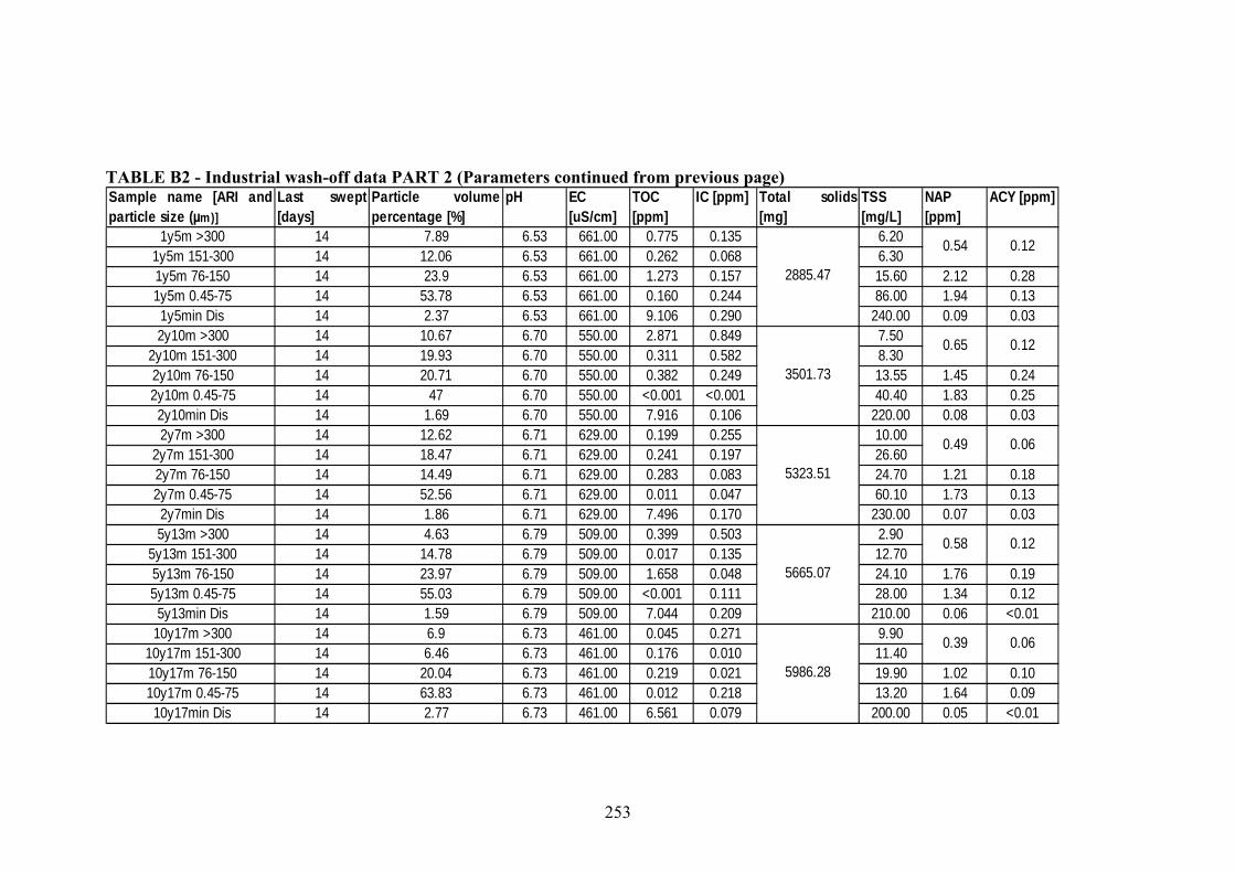
253
TABLE B2 - Industrial wash-off data PART 2 (Parameters continued from previous page)
1y5m >300 14 7.89 6.53 661.00 0.775 0.135 6.20 1y5m 151-300 14 12.06 6.53 661.00 0.262 0.068 6.30 1y5m 76-150 14 23.9 6.53 661.00 1.273 0.157 15.60 2.12 0.28 1y5m 0.45-75 14 53.78 6.53 661.00 0.160 0.244 86.00 1.94 0.13 1y5min Dis 14 2.37 6.53 661.00 9.106 0.290 240.00 0.09 0.03 2y10m >300 14 10.67 6.70 550.00 2.871 0.849 7.50
2y10m 151-300 14 19.93 6.70 550.00 0.311 0.582 8.30 2y10m 76-150 14 20.71 6.70 550.00 0.382 0.249 13.55 1.45 0.24 2y10m 0.45-75 14 47 6.70 550.00 <0.001 <0.001 40.40 1.83 0.25 2y10min Dis 14 1.69 6.70 550.00 7.916 0.106 220.00 0.08 0.03 2y7m >300 14 12.62 6.71 629.00 0.199 0.255 10.00
2y7m 151-300 14 18.47 6.71 629.00 0.241 0.197 26.60 2y7m 76-150 14 14.49 6.71 629.00 0.283 0.083 24.70 1.21 0.18 2y7m 0.45-75 14 52.56 6.71 629.00 0.011 0.047 60.10 1.73 0.13 2y7min Dis 14 1.86 6.71 629.00 7.496 0.170 230.00 0.07 0.03 5y13m >300 14 4.63 6.79 509.00 0.399 0.503 2.90
5y13m 151-300 14 14.78 6.79 509.00 0.017 0.135 12.70 5y13m 76-150 14 23.97 6.79 509.00 1.658 0.048 24.10 1.76 0.19 5y13m 0.45-75 14 55.03 6.79 509.00 <0.001 0.111 28.00 1.34 0.12 5y13min Dis 14 1.59 6.79 509.00 7.044 0.209 210.00 0.06 <0.01
10y17m >300 14 6.9 6.73 461.00 0.045 0.271 9.90 10y17m 151-300 14 6.46 6.73 461.00 0.176 0.010 11.40 10y17m 76-150 14 20.04 6.73 461.00 0.219 0.021 19.90 1.02 0.10 10y17m 0.45-75 14 63.83 6.73 461.00 0.012 0.218 13.20 1.64 0.09 10y17min Dis 14 2.77 6.73 461.00 6.561 0.079 200.00 0.05 <0.01
Sample name [ARI andparticle size (µm)]
Last swept[days]
Particle volumepercentage [%]
pH EC [uS/cm]
TOC [ppm]
IC [ppm] Total solids[mg]
TSS [mg/L]
NAP [ppm]
ACY [ppm]
2885.47
0.54 0.12
3501.73
0.65 0.12
5323.51
0.49 0.06
5665.07
0.58 0.12
5986.28
0.39 0.06

254
TABLE B2 - Industrial wash-off data PART 2 (Parameters continued from previous page)
1y5m >300 1y5m 151-300 1y5m 76-150 0.25 0.05 0.05 0.05 0.07 0.09 0.09 0.06 0.05 0.09 1y5m 0.45-75 0.31 0.06 0.07 0.06 0.20 0.21 0.13 0.23 0.07 0.11 1y5min Dis 0.02 0.01 <0.01 <0.01 0.02 <0.01 0.01 <0.01 <0.01 0.01 2y10m >300
2y10m 151-300 2y10m 76-150 0.26 0.05 0.06 0.06 0.07 0.09 0.09 0.14 0.04 0.07 2y10m 0.45-75 0.31 0.10 0.08 0.06 0.19 0.24 0.12 0.25 0.07 0.10 2y10min Dis 0.02 <0.01 <0.01 <0.01 0.02 <0.01 0.01 <0.01 <0.01 0.01 2y7m >300
2y7m 151-300 2y7m 76-150 0.16 0.05 0.05 0.05 0.06 0.08 0.06 0.09 0.03 0.04 2y7m 0.45-75 0.21 0.05 0.08 0.03 0.12 0.13 0.10 0.21 0.06 0.04 2y7min Dis 0.02 <0.01 <0.01 <0.01 0.02 <0.01 <0.01 <0.01 <0.01 <0.01 5y13m >300
5y13m 151-300 5y13m 76-150 0.18 0.07 0.05 0.05 0.06 0.03 0.06 0.10 0.03 0.03 5y13m 0.45-75 0.20 0.05 0.09 0.04 0.12 0.21 0.10 0.24 0.06 0.10 5y13min Dis 0.02 <0.01 <0.01 <0.01 0.01 <0.01 <0.01 <0.01 <0.01 <0.01 10y17m >300
10y17m 151-300 10y17m 76-150 0.10 0.06 0.05 0.03 0.05 0.02 0.06 0.10 0.04 0.04 10y17m 0.45-75 0.21 0.04 0.05 0.03 0.10 0.20 0.11 0.27 0.07 0.11 10y17min Dis <0.01 <0.01 <0.01 <0.01 0.01 <0.01 <0.01 <0.01 <0.01 <0.01
Sample name [ARI andparticle size (µm)]
ACE [ppm] FLU [ppm] PHE [ppm] CHR [ppm]
BbF [ppm] BaP [ppm]ANT [ppm]
FLA [ppm] PYR [ppm] BaA [ppm]
<0.01 0.03 0.01 <0.01
0.10 0.05 0.08
0.08 0.07 0.07
<0.01 0.03 0.01 <0.01 0.08 0.02 0.07
0.02 0.090.05
<0.01 <0.01 <0.01 <0.01
0.05 <0.01 0.06
0.05 0.03 0.06
0.02 0.01 <0.01 <0.01 0.07 0.02 0.06
0.01 0.050.03
<0.01 <0.01 <0.01 <0.01 <0.01 0.050.03 0.01 0.04 0.07

255
TABLE B2 - Industrial wash-off data PART 2 (Parameters continued from previous page)
1y5m >300 0.088 0.015 0.043 0.002 0.012 <0.001 0.003 0.001 1y5m 151-300 0.080 0.013 0.040 0.002 0.014 <0.001 0.001 0.001 1y5m 76-150 <0.01 <0.01 0.02 0.176 0.026 0.104 0.005 0.016 <0.001 0.006 0.002 1y5m 0.45-75 0.03 <0.01 0.02 0.488 0.035 0.280 0.014 0.018 <0.001 0.002 0.005 1y5min Dis <0.01 <0.01 0.01 <0.005 0.510 0.014 0.002 0.010 <0.001 <0.001 0.017 2y10m >300 0.057 0.013 0.025 0.002 0.005 <0.001 0.001 0.001
2y10m 151-300 0.073 0.014 0.036 0.002 0.014 <0.001 0.001 0.001 2y10m 76-150 <0.01 <0.01 0.02 0.144 0.018 0.072 0.004 0.016 <0.001 0.003 0.002 2y10m 0.45-75 0.02 <0.01 0.02 0.304 0.026 0.168 0.010 0.017 <0.001 0.001 0.003 2y10min Dis <0.01 <0.01 <0.01 <0.005 0.380 0.009 0.001 0.008 <0.001 <0.001 0.011 2y7m >300 0.078 0.012 0.034 0.002 0.007 <0.001 <0.001 0.001
2y7m 151-300 0.078 0.011 0.036 0.002 0.011 <0.001 <0.001 0.001 2y7m 76-150 <0.01 <0.01 0.01 0.208 0.019 0.104 0.006 0.013 <0.001 0.001 0.002 2y7m 0.45-75 0.01 <0.01 <0.01 0.880 0.051 0.416 0.025 0.039 <0.001 0.002 0.010 2y7min Dis <0.01 <0.01 <0.01 <0.005 0.340 0.007 0.001 0.008 <0.001 <0.001 0.013 5y13m >300 0.058 0.008 0.027 0.001 0.004 <0.001 <0.001 0.001
5y13m 151-300 0.066 0.011 0.034 0.002 0.009 <0.001 0.001 0.001 5y13m 76-150 <0.01 <0.01 <0.01 0.224 0.018 0.104 0.005 0.011 <0.001 0.001 0.004 5y13m 0.45-75 0.01 <0.01 <0.01 0.600 0.034 0.280 0.014 0.026 <0.001 0.001 0.006 5y13min Dis <0.01 <0.01 <0.01 <0.005 0.260 <0.005 <0.001 0.008 <0.001 <0.001 0.017
10y17m >300 0.041 0.015 0.034 0.004 0.003 0.001 0.001 0.002 10y17m 151-300 0.054 0.011 0.032 0.002 0.010 0.001 0.001 0.002 10y17m 76-150 <0.01 <0.01 <0.01 0.152 0.017 0.078 0.005 0.010 0.001 0.001 0.003 10y17m 0.45-75 <0.01 <0.01 <0.01 0.488 0.028 0.248 0.014 0.027 <0.001 0.001 0.005 10y17min Dis <0.01 <0.01 <0.01 <0.005 0.290 <0.005 <0.001 0.006 <0.001 <0.001 0.009
<0.01 <0.01
<0.01
<0.01
<0.01
<0.01
<0.01
<0.01 <0.01
<0.01 <0.01
<0.01 <0.01
<0.01 <0.01
Cu [ppm] Cd [ppm] Cr [ppm] Mn [ppm]
Fe [ppm] Zn [ppm] Al [ppm] Pb [ppm]Sample name [ARI andparticle size (µm)]
IND [ppm] DbA [ppm] BgP [ppm]

256
TABLE B2 – Industrial Wash-off data PART 3 (Blanks and replicates)
Field blank 15/10/2003 115 - Field BLANK - - - - - -Field blank 15/10/2003 115 - Field BLANK - - - - - -Field blank 15/10/2003 86 - Field BLANK - - - - - -Field blank 15/10/2003 86 - Field BLANK - - - - - -Field blank 15/10/2003 133 - Field BLANK - - - - - -Field blank 15/10/2003 133 - Field BLANK - - - - - -Field blank 15/10/2003 65 - Field BLANK - - - - - -Field blank 15/10/2003 65 - Field BLANK - - - - - -
Laboratory blank 15/10/2003 - - Distilled Blank - - - - - -Laboratory blank 15/10/2003 - - Distilled Blank - - - - - -
Build-up U/S St 76-150 15/10/2003 - - Replicate - - - - - -Build-up U/S St <0.45 15/10/2003 - - Replicate - - - - - -
1y5m 76-150 15/10/2003 115 5 Replicate - - - - - -10y65min 0.45-75 15/10/2003 65 65 Replicate - - - - - -
Sample name Sample date Intensity [mm/hr]
Duration [min]
Classification
Dry daysbefore
Last rainfall
Event Total volumeevent [L]
Slope [m/m]
Texture depth
Field blank - - 6.65 530.00 4.274 1.005 <0.01 <0.01 <0.01Field blank - - 6.65 530.00 <0.001 <0.001 0.04 0.065 <0.01Field blank - - 6.75 460.00 1.001 1.276 <0.01 <0.01 <0.01Field blank - - 6.75 460.00 <0.001 <0.001 0.02 0.057 <0.01Field blank - - 6.72 460.00 0.740 0.650 <0.01 <0.01 <0.01Field blank - - 6.72 460.00 <0.001 <0.001 <0.01 0.023 <0.01Field blank - - 6.61 340.00 3.426 0.294 <0.01 <0.01 <0.01Field blank - - 6.61 340.00 <0.001 <0.001 0.02 0.032 <0.01
Laboratory blank - - 6.27 9.00 <0.001 <0.001 <0.01 <0.01 <0.01Laboratory blank - - 6.27 9.00 <0.001 <0.001 <0.01 0.012 <0.01
Build-up U/S St 76-150 - - - - 0.639 <0.001 225.1 2.202 0.351Build-up U/S St <0.45 - - - - 8.25 <0.001 30 0.062 0.023
1y5m 76-150 - - - - 1.197 0.152 17.1 2.119 0.27610y65min 0.45-75 - - - - 1.21 0.158 14.2 2.102 0.191
ACY [ppm]TOC [ppm]
IC [ppm]
TSS [mg/L]
pH EC [uS/cm]
NAP [ppm]Sample name Last swept
Particle volumepercentage [%]

257
TABLE B2 – Industrial Wash-off data PART 3 (Blanks and replicates continued from previous page)
Field blank <0.01 <0.01 <0.01 <0.01 <0.01 <0.01 <0.01 <0.01 <0.01Field blank <0.01 <0.01 <0.01 <0.01 <0.01 <0.01 <0.01 <0.01 <0.01Field blank <0.01 <0.01 <0.01 <0.01 <0.01 <0.01 <0.01 <0.01 <0.01Field blank <0.01 <0.01 <0.01 <0.01 <0.01 <0.01 <0.01 <0.01 <0.01Field blank <0.01 <0.01 <0.01 <0.01 <0.01 <0.01 <0.01 <0.01 <0.01Field blank <0.01 <0.01 <0.01 <0.01 <0.01 <0.01 <0.01 <0.01 <0.01Field blank <0.01 <0.01 <0.01 <0.01 <0.01 <0.01 <0.01 <0.01 <0.01Field blank <0.01 <0.01 <0.01 <0.01 <0.01 <0.01 <0.01 <0.01 <0.01
Laboratory blank <0.01 <0.01 <0.01 <0.01 <0.01 <0.01 <0.01 <0.01 <0.01Laboratory blank <0.01 <0.01 <0.01 <0.01 <0.01 <0.01 <0.01 <0.01 <0.01
Build-up U/S St 76-150 0.40 0.12 0.14 0.10 0.10 0.16 0.16 0.32 0.12Build-up U/S St <0.45 0.02 <0.01 <0.01 <0.01 0.02 <0.01 <0.01 <0.01 <0.01
1y5m 76-150 0.25 0.05 0.05 0.06 0.07 0.09 0.09 0.06 0.05 10y65min 0.45-75 0.32 0.02 0.12 0.07 0.18 0.12 0.12 <0.01 0.05
Sample name ACE [ppm] FLU [ppm]
PHE [ppm] CHR [ppm]
BbF [ppm]ANT [ppm] FLA [ppm] PYR [ppm]
BaA [ppm]
Field blank <0.01 <0.01 <0.01 <0.01 <0.005 0.015 <0.005 <0.001 <0.001 <0.001 <0.001 0.001Field blank <0.01 <0.01 <0.01 <0.01 0.016 0.008 <0.005 0.001 0.001 0.001 <0.001 0.001Field blank <0.01 <0.01 <0.01 <0.01 <0.005 0.016 <0.005 <0.001 <0.001 <0.001 <0.001 <0.001Field blank <0.01 <0.01 <0.01 <0.01 0.008 0.005 <0.005 <0.001 <0.001 <0.001 <0.001 <0.001Field blank <0.01 <0.01 <0.01 <0.01 <0.005 0.015 <0.005 <0.001 <0.001 <0.001 <0.001 <0.001Field blank <0.01 <0.01 <0.01 <0.01 0.006 0.005 0.005 <0.001 <0.001 <0.001 <0.001 <0.001Field blank <0.01 <0.01 <0.01 <0.01 <0.005 0.007 <0.005 <0.001 <0.001 <0.001 <0.001 0.001Field blank <0.01 <0.01 <0.01 <0.01 0.006 0.002 0.008 0.001 <0.001 <0.001 <0.001 <0.001
Laboratory blank <0.01 <0.01 <0.01 <0.01 <0.005 0.004 <0.005 <0.001 <0.001 <0.001 <0.001 <0.001Laboratory blank <0.01 <0.01 <0.01 <0.01 0.002 0.007 <0.005 <0.001 <0.001 <0.001 <0.001 <0.001
Build-up U/S St 76-150 0.15 <0.01 <0.01 0.02 2.230 0.113 0.630 0.036 0.037 <0.001 0.003 0.021Build-up U/S St <0.45 <0.01 <0.01 <0.01 <0.01 <0.005 0.180 0.009 0.002 0.007 <0.001 <0.001 0.023
1y5m 76-150 0.09 <0.01 <0.01 0.02 0.178 0.026 0.103 0.005 0.016 <0.001 0.006 0.002 10y65min 0.45-75 0.14 0.01 <0.01 0.02 0.150 0.019 0.099 0.004 0.022 <0.001 0.002 0.002
Sample name Fe [ppm]
Zn [ppm]
BaP [ppm]
IND [ppm]
DbA [ppm]
BgP [ppm]
Cr [ppm]
Mn [ppm]
Al [ppm] Pb [ppm]
Cu [ppm]
Cd [ppm]

258
TABLE B3 – Commercial Wash-off data PART 1 (Data for simulated rainfall events with intensities 65 and 86mm/hr)
1y20min >300 11/01/2004 65 20 EMC 1 year 20 min 24 0.05 0.92 0 1y20min 151-300 11/01/2004 65 20 EMC 1 year 20 min 24 0.05 0.92 0 1y20min 76-150 11/01/2004 65 20 EMC 1 year 20 min 24 0.05 0.92 0 1y20min 0.45-75 11/01/2004 65 20 EMC 1 year 20 min 24 0.05 0.92 0
1y20min Dis 11/01/2004 65 20 EMC 1 year 20 min 24 0.05 0.92 0 2y35min >300 11/01/2004 65 35 EMC 2 year 35 min 40 0.05 0.92 0
2y35min 151-300 11/01/2004 65 35 EMC 2 year 35 min 40 0.05 0.92 0 2y35min 76-150 11/01/2004 65 35 EMC 2 year 35 min 40 0.05 0.92 0 2y35min 0.45-75 11/01/2004 65 35 EMC 2 year 35 min 40 0.05 0.92 0
2y35min Dis 11/01/2004 65 35 EMC 2 year 35 min 40 0.05 0.92 0 10y65min >300 11/01/2004 65 65 EMC 10 year 65 min 73 0.05 0.92 0
10y65min 151-300 11/01/2004 65 65 EMC 10 year 65 min 73 0.05 0.92 0 10y65min 76-150 11/01/2004 65 65 EMC 10 year 65 min 73 0.05 0.92 0 10y65min 0.45-75 11/01/2004 65 65 EMC 10 year 65 min 73 0.05 0.92 0
10y65min Dis 11/01/2004 65 65 EMC 10 year 65 min 73 0.05 0.92 0 1y10m >300 11/01/2004 86 10 EMC 1 year 10 min 40 0.02 0.92 0
1y10m 151-300 11/01/2004 86 10 EMC 1 year 10 min 40 0.02 0.92 0 1y10m 76-150 11/01/2004 86 10 EMC 1 year 10 min 40 0.02 0.92 0 1y10m 0.45-75 11/01/2004 86 10 EMC 1 year 10 min 40 0.02 0.92 0 1y10min Dis 11/01/2004 86 10 EMC 1 year 10 min 40 0.02 0.92 0 2y20m >300 11/01/2004 86 20 EMC 2 year 20 min 78 0.02 0.92 0
2y20m 151-300 11/01/2004 86 20 EMC 2 year 20 min 78 0.02 0.92 0 2y20m 76-150 11/01/2004 86 20 EMC 2 year 20 min 78 0.02 0.92 0 2y20m 0.45-75 11/01/2004 86 20 EMC 2 year 20 min 78 0.02 0.92 0 2y20min Dis 11/01/2004 86 20 EMC 2 year 20 min 78 0.02 0.92 0 10y40m >300 11/01/2004 86 40 EMC 10 year 40 min 145 0.02 0.92 0
10y40m 151-300 11/01/2004 86 40 EMC 10 year 40 min 145 0.02 0.92 0 10y40m 76-150 11/01/2004 86 40 EMC 10 year 40 min 145 0.02 0.92 0 10y40m 0.45-75 11/01/2004 86 40 EMC 10 year 40 min 145 0.02 0.92 0 10y40min Dis 11/01/2004 86 40 EMC 10 year 40 min 145 0.02 0.92 0
Sample name [ARI andparticle size (µm)]
Sample date Intensity [mm/hr]
Duration [min]
Dry daysbefore
Event Total volume [L]
Slope [m/m]
Texture depth [mm]

259
TABLE B3 - Commercial wash-off data PART 1 (Parameters continued from previous page)
1y20min >300 Unknown 0 6.62 26.90 1.225 1.930 17.00 1y20min 151-300 Unknown 7.14 6.62 26.90 <0.001 0.532 19.30 1y20min 76-150 Unknown 19.22 6.62 26.90 <0.001 <0.001 22.90 1y20min 0.45-75 Unknown 73.64 6.62 26.90 1.062 <0.001 33.80
1y20min Dis Unknown <0.01 6.62 26.90 5.815 <0.001 20.00 2y35min >300 Unknown 9.54 7.20 31.10 <0.001 <0.001 42.10
2y35min 151-300 Unknown 14.91 7.20 31.10 <0.001 <0.001 49.50 2y35min 76-150 Unknown 26.13 7.20 31.10 <0.001 <0.001 16.60 2y35min 0.45-75 Unknown 42.59 7.20 31.10 2.934 <0.001 23.00
2y35min Dis Unknown 6.83 7.20 31.10 1.621 <0.001 20.00 10y65min >300 Unknown 10.73 7.09 32.70 3.885 <0.001 22.90
10y65min 151-300 Unknown 12.32 7.09 32.70 <0.001 <0.001 25.40 10y65min 76-150 Unknown 23.65 7.09 32.70 <0.001 <0.001 20.20 10y65min 0.45-75 Unknown 50.57 7.09 32.70 <0.001 <0.001 16.80
10y65min Dis Unknown 3.87 7.09 32.70 1.621 <0.001 10.00 1y10m >300 Unknown 7.06 7.66 46.40 0.968 0.602 14.70
1y10m 151-300 Unknown 12.74 7.66 46.40 0.189 <0.001 30.60 1y10m 76-150 Unknown 32.31 7.66 46.40 <0.001 <0.001 27.60 1y10m 0.45-75 Unknown 41.89 7.66 46.40 <0.001 <0.001 21.80 1y10min Dis Unknown 1 7.66 46.40 7.340 <0.001 20.00 2y20m >300 Unknown 21.02 7.54 52.60 0.171 0.068 20.80
2y20m 151-300 Unknown 15.01 7.54 52.60 0.080 0.211 23.00 2y20m 76-150 Unknown 26.66 7.54 52.60 <0.001 0.031 28.80 2y20m 0.45-75 Unknown 36.1 7.54 52.60 0.601 0.046 27.70 2y20min Dis Unknown 1.21 7.54 52.60 6.606 0.793 40.00 10y40m >300 Unknown 11.3 6.82 46.40 <0.001 <0.001 13.50
10y40m 151-300 Unknown 19.5 6.82 46.40 <0.001 0.106 29.10 10y40m 76-150 Unknown 28.87 6.82 46.40 <0.001 0.087 22.80 10y40m 0.45-75 Unknown 38.91 6.82 46.40 0.687 <0.001 21.40 10y40min Dis Unknown 1.42 6.82 46.40 5.667 0.286 30.00
TSS [mg/L]
2232.00
5248.00
pH EC [uS/cm]
TOC [ppm]
IC [ppm]
Total solids[mg]
12586.00
Sample name [ARIand particle size (µm)]
Last swept[days]
Particle volumepercentage [%]
6226.90
3788.00
7823.40

260
TABLE B3 - Commercial wash-off data PART 1 (Parameters continued from previous page)
1y20min >300 1y20min 151-300 1y20min 76-150 1.08 0.34 0.06 0.05 0.12 0.02 0.06 0.10 0.32 0.23 1y20min 0.45-75 4.05 0.45 0.10 0.10 0.12 0.03 0.17 0.34 0.41 0.12
1y20min Dis 0.12 0.01 <0.01 <0.01 <0.01 <0.01 <0.01 <0.01 0.02 <0.01 2y35min >300
2y35min 151-300 2y35min 76-150 0.87 0.21 0.04 0.03 0.08 <0.01 <0.01 0.09 0.21 0.12 2y35min 0.45-75 6.45 0.57 0.76 0.53 1.03 0.08 0.20 0.66 0.43 0.20
2y35min Dis 0.01 <0.01 <0.01 <0.01 0.01 <0.01 <0.01 <0.01 0.01 <0.01 10y65min >300
10y65min 151-300 10y65min 76-150 0.76 0.21 0.07 0.08 0.04 <0.01 <0.01 0.03 0.22 0.12 10y65min 0.45-75 3.46 0.35 0.34 0.10 0.10 <0.01 0.16 0.24 0.25 0.43
10y65min Dis 0.01 <0.01 <0.01 <0.01 <0.01 <0.01 0.01 <0.01 <0.01 <0.01 1y10m >300
1y10m 151-300 1y10m 76-150 1.65 0.54 0.15 0.02 <0.01 <0.01 <0.01 0.04 0.15 0.14 1y10m 0.45-75 4.76 0.45 0.10 0.08 0.09 0.02 0.12 0.28 0.32 0.09 1y10min Dis 0.24 0.02 0.01 <0.01 <0.01 0.01 0.01 <0.01 0.02 0.01 2y20m >300
2y20m 151-300 2y20m 76-150 0.95 0.42 0.12 <0.01 <0.01 <0.01 <0.01 0.02 0.03 0.01 2y20m 0.45-75 4.97 0.54 0.12 0.10 0.11 0.16 0.14 0.31 0.41 0.12 2y20min Dis 0.10 0.01 <0.01 <0.01 <0.01 0.01 0.01 <0.01 0.01 <0.01 10y40m >300
10y40m 151-300 10y40m 76-150 0.87 0.25 0.07 <0.01 <0.01 <0.01 <0.01 <0.01 <0.01 <0.01 10y40m 0.45-75 4.01 0.54 0.13 0.09 0.10 0.17 0.14 0.27 0.39 0.22 10y40min Dis 0.02 <0.01 <0.01 <0.01 <0.01 0.01 <0.01 <0.01 <0.01 <0.01
BaP
[ppm]
<0.01
<0.01
<0.01
<0.01
0.22
0.10
<0.01<0.01 <0.01 0.06 0.140.96 0.25 0.02 0.02
0.13
1.35 0.33 0.10 0.10 0.08 0.02 0.16 0.23 0.10
0.04 0.08 0.13 0.241.12 0.35 0.12 0.07
0.08
0.76 0.17 0.03 <0.01 <0.01 <0.01 0.10 0.12 <0.01
PYR [ppm] BaA [ppm]
1.03 0.32 0.09 0.04 <0.01 <0.01 0.12 0.23
FLU [ppm] PHE [ppm] ANT
[ppm]
FLA [ppm]Sample name [ARI and
particle size (µm)]
NAP [ppm] ACY [ppm] ACE [ppm]
0.27 0.13 <0.01 <0.01 <0.01<0.01 <0.01 0.06 0.08
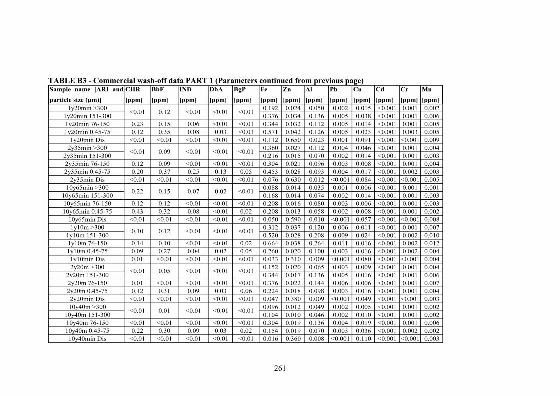
261
TABLE B3 - Commercial wash-off data PART 1 (Parameters continued from previous page)
1y20min >300 0.192 0.024 0.050 0.002 0.015 <0.001 0.001 0.002 1y20min 151-300 0.376 0.034 0.136 0.005 0.038 <0.001 0.001 0.006 1y20min 76-150 0.23 0.15 0.06 <0.01 <0.01 0.344 0.032 0.112 0.005 0.014 <0.001 0.001 0.005 1y20min 0.45-75 0.12 0.35 0.08 0.03 <0.01 0.571 0.042 0.126 0.005 0.023 <0.001 0.003 0.005
1y20min Dis <0.01 <0.01 <0.01 <0.01 <0.01 0.112 0.650 0.023 0.001 0.091 <0.001 <0.001 0.009 2y35min >300 0.360 0.027 0.112 0.004 0.046 <0.001 0.001 0.004
2y35min 151-300 0.216 0.015 0.070 0.002 0.014 <0.001 0.001 0.003 2y35min 76-150 0.12 0.09 <0.01 <0.01 <0.01 0.304 0.021 0.096 0.003 0.008 <0.001 0.001 0.004 2y35min 0.45-75 0.20 0.37 0.25 0.13 0.05 0.453 0.028 0.093 0.004 0.017 <0.001 0.002 0.003
2y35min Dis <0.01 <0.01 <0.01 <0.01 <0.01 0.076 0.630 0.012 <0.001 0.084 <0.001 <0.001 0.005 10y65min >300 0.088 0.014 0.035 0.001 0.006 <0.001 0.001 0.001
10y65min 151-300 0.168 0.014 0.074 0.002 0.014 <0.001 0.001 0.003 10y65min 76-150 0.12 0.12 <0.01 <0.01 <0.01 0.208 0.016 0.080 0.003 0.006 <0.001 0.001 0.003 10y65min 0.45-75 0.43 0.32 0.08 <0.01 0.02 0.208 0.013 0.058 0.002 0.008 <0.001 0.001 0.002
10y65min Dis <0.01 <0.01 <0.01 <0.01 <0.01 0.050 0.590 0.010 <0.001 0.057 <0.001 <0.001 0.008 1y10m >300 0.312 0.037 0.120 0.006 0.011 <0.001 0.001 0.007
1y10m 151-300 0.520 0.028 0.208 0.009 0.024 <0.001 0.002 0.010 1y10m 76-150 0.14 0.10 <0.01 <0.01 0.02 0.664 0.038 0.264 0.011 0.016 <0.001 0.002 0.012 1y10m 0.45-75 0.09 0.27 0.04 0.02 0.05 0.260 0.020 0.100 0.003 0.016 <0.001 0.002 0.004 1y10min Dis 0.01 <0.01 <0.01 <0.01 <0.01 0.033 0.310 0.009 <0.001 0.080 <0.001 <0.001 0.004 2y20m >300 0.152 0.020 0.065 0.003 0.009 <0.001 0.001 0.004
2y20m 151-300 0.344 0.017 0.136 0.005 0.016 <0.001 0.001 0.006 2y20m 76-150 0.01 <0.01 <0.01 <0.01 <0.01 0.376 0.022 0.144 0.006 0.006 <0.001 0.001 0.007 2y20m 0.45-75 0.12 0.31 0.09 0.03 0.06 0.224 0.018 0.098 0.003 0.016 <0.001 0.001 0.004 2y20min Dis <0.01 <0.01 <0.01 <0.01 <0.01 0.047 0.380 0.009 <0.001 0.049 <0.001 <0.001 0.003 10y40m >300 0.096 0.012 0.049 0.002 0.005 <0.001 0.001 0.002
10y40m 151-300 0.104 0.010 0.046 0.002 0.010 <0.001 0.001 0.002 10y40m 76-150 <0.01 <0.01 <0.01 <0.01 <0.01 0.304 0.019 0.136 0.004 0.019 <0.001 0.001 0.006 10y40m 0.45-75 0.22 0.30 0.09 0.03 0.02 0.154 0.019 0.070 0.003 0.036 <0.001 0.002 0.002 10y40min Dis <0.01 <0.01 <0.01 <0.01 <0.01 0.016 0.360 0.008 <0.001 0.110 <0.001 <0.001 0.003
Mn
[ppm]
Pb
[ppm]
Cu
[ppm]
Cd
[ppm]
Cr
[ppm]
Fe
[ppm]
<0.01 <0.01<0.01 0.01 <0.01
Al
[ppm]
<0.01 <0.01
Sample name [ARI and
particle size (µm)]
CHR
[ppm]
BbF
[ppm]
Zn
[ppm]
IND
[ppm]
DbA
[ppm]
BgP
[ppm]
<0.01
<0.01 0.12 <0.01
<0.01 0.09 <0.01 <0.01
<0.01 <0.01
0.22 0.15
0.10 0.12 <0.01
0.07 0.02 <0.01
<0.01 <0.01<0.01 0.05 <0.01

262
TABLE B3 - Commercial Wash-off data PART 2 (Data for simulated rainfall events with intensities 115 and 133mm/hr)
1y5m >300 11/01/2004 115 5 EMC 1 year 5 min 11 0.03 0.92 0 Unknown 1y5m 151-300 11/01/2004 115 5 EMC 1 year 5 min 11 0.03 0.92 0 Unknown 1y5m 76-150 11/01/2004 115 5 EMC 1 year 5 min 11 0.03 0.92 0 Unknown 1y5m 0.45-75 11/01/2004 115 5 EMC 1 year 5 min 11 0.03 0.92 0 Unknown 1y5min Dis 11/01/2004 115 5 EMC 1 year 5 min 11 0.03 0.92 0 Unknown 2y10m >300 11/01/2004 115 10 EMC 2 year 10 min 23 0.03 0.92 0 Unknown
2y10m 151-300 11/01/2004 115 10 EMC 2 year 10 min 23 0.03 0.92 0 Unknown 2y10m 76-150 11/01/2004 115 10 EMC 2 year 10 min 23 0.03 0.92 0 Unknown 2y10m 0.45-75 11/01/2004 115 10 EMC 2 year 10 min 23 0.03 0.92 0 Unknown 2y10min Dis 11/01/2004 115 10 EMC 2 year 10 min 23 0.03 0.92 0 Unknown 10y25m >300 11/01/2004 115 25 EMC 10 year 25 min 48 0.03 0.92 0 Unknown
10y25 151-300 11/01/2004 115 25 EMC 10 year 25 min 48 0.03 0.92 0 Unknown 10y25 76-150 11/01/2004 115 25 EMC 10 year 25 min 48 0.03 0.92 0 Unknown 10y25 0.45-75 11/01/2004 115 25 EMC 10 year 25 min 48 0.03 0.92 0 Unknown 10y25min Dis 11/01/2004 115 25 EMC 10 year 25 min 48 0.03 0.92 0 Unknown
2y7m >300 11/01/2004 133 7 EMC 2 year 7 min 25 0.04 0.92 0 Unknown 2y7m 151-300 11/01/2004 133 7 EMC 2 year 7 min 25 0.04 0.92 0 Unknown 2y7m 76-150 11/01/2004 133 7 EMC 2 year 7 min 25 0.04 0.92 0 Unknown 2y7m 0.45-75 11/01/2004 133 7 EMC 2 year 7 min 25 0.04 0.92 0 Unknown 2y7min Dis 11/01/2004 133 7 EMC 2 year 7 min 25 0.04 0.92 0 Unknown 5y13m >300 11/01/2004 133 13 EMC 5 year 13 min 76 0.04 0.92 0 Unknown
5y13m 151-300 11/01/2004 133 13 EMC 5 year 13 min 76 0.04 0.92 0 Unknown 5y13m 76-150 11/01/2004 133 13 EMC 5 year 13 min 76 0.04 0.92 0 Unknown 5y13m 0.45-75 11/01/2004 133 13 EMC 5 year 13 min 76 0.04 0.92 0 Unknown 5y13min Dis 11/01/2004 133 13 EMC 5 year 13 min 76 0.04 0.92 0 Unknown 10y17m >300 11/01/2004 133 17 EMC 10 year 17 min 138 0.04 0.92 0 Unknown
10y17m 151-300 11/01/2004 133 17 EMC 10 year 17 min 138 0.04 0.92 0 Unknown 10y17m 76-150 11/01/2004 133 17 EMC 10 year 17 min 138 0.04 0.92 0 Unknown 10y17m 0.45-75 11/01/2004 133 17 EMC 10 year 17 min 138 0.04 0.92 0 Unknown 10y17min Dis 11/01/2004 133 17 EMC 10 year 17 min 138 0.04 0.92 0 Unknown
Dry days
before
Last swept
[days]
Event Total volume
event [L]
Slope
[m/m]
Texture depth [mm]
Sample name [ARIand particle size(µm)]
Sample date Intensity
[mm/hr]
Duration
[min]
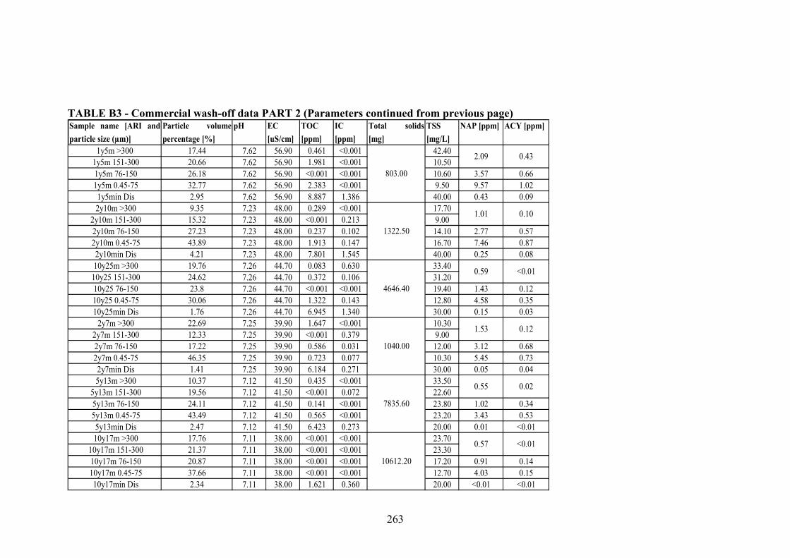
263
TABLE B3 - Commercial wash-off data PART 2 (Parameters continued from previous page)
1y5m >300 17.44 7.62 56.90 0.461 <0.001 42.40 1y5m 151-300 20.66 7.62 56.90 1.981 <0.001 10.50 1y5m 76-150 26.18 7.62 56.90 <0.001 <0.001 10.60 3.57 0.66 1y5m 0.45-75 32.77 7.62 56.90 2.383 <0.001 9.50 9.57 1.02 1y5min Dis 2.95 7.62 56.90 8.887 1.386 40.00 0.43 0.09 2y10m >300 9.35 7.23 48.00 0.289 <0.001 17.70
2y10m 151-300 15.32 7.23 48.00 <0.001 0.213 9.00 2y10m 76-150 27.23 7.23 48.00 0.237 0.102 14.10 2.77 0.57 2y10m 0.45-75 43.89 7.23 48.00 1.913 0.147 16.70 7.46 0.87 2y10min Dis 4.21 7.23 48.00 7.801 1.545 40.00 0.25 0.08 10y25m >300 19.76 7.26 44.70 0.083 0.630 33.40 10y25 151-300 24.62 7.26 44.70 0.372 0.106 31.20 10y25 76-150 23.8 7.26 44.70 <0.001 <0.001 19.40 1.43 0.12 10y25 0.45-75 30.06 7.26 44.70 1.322 0.143 12.80 4.58 0.35 10y25min Dis 1.76 7.26 44.70 6.945 1.340 30.00 0.15 0.03
2y7m >300 22.69 7.25 39.90 1.647 <0.001 10.30 2y7m 151-300 12.33 7.25 39.90 <0.001 0.379 9.00 2y7m 76-150 17.22 7.25 39.90 0.586 0.031 12.00 3.12 0.68 2y7m 0.45-75 46.35 7.25 39.90 0.723 0.077 10.30 5.45 0.73 2y7min Dis 1.41 7.25 39.90 6.184 0.271 30.00 0.05 0.04 5y13m >300 10.37 7.12 41.50 0.435 <0.001 33.50
5y13m 151-300 19.56 7.12 41.50 <0.001 0.072 22.60 5y13m 76-150 24.11 7.12 41.50 0.141 <0.001 23.80 1.02 0.34 5y13m 0.45-75 43.49 7.12 41.50 0.565 <0.001 23.20 3.43 0.53 5y13min Dis 2.47 7.12 41.50 6.423 0.273 20.00 0.01 <0.01 10y17m >300 17.76 7.11 38.00 <0.001 <0.001 23.70
10y17m 151-300 21.37 7.11 38.00 <0.001 <0.001 23.30 10y17m 76-150 20.87 7.11 38.00 <0.001 <0.001 17.20 0.91 0.14 10y17m 0.45-75 37.66 7.11 38.00 <0.001 <0.001 12.70 4.03 0.15 10y17min Dis 2.34 7.11 38.00 1.621 0.360 20.00 <0.01 <0.01
10612.20
0.57 <0.01
1040.00
1.53 0.12
7835.60
0.55 0.02
1322.50
1.01 0.10
4646.40
0.59 <0.01
NAP [ppm] ACY [ppm]
803.00
2.09 0.43
TOC [ppm]
IC [ppm]
Total solids[mg]
TSS [mg/L]
Sample name [ARI andparticle size (µm)]
Particle volumepercentage [%]
pH EC [uS/cm]

264
TABLE B3 - Commercial wash-off data PART 2 (Parameters continued from previous page)
1y5m >300 1y5m 151-300 1y5m 76-150 0.16 0.12 0.98 0.07 0.25 0.12 0.31 0.27 0.13 0.18 1y5m 0.45-75 0.19 0.65 1.34 0.12 0.66 0.34 0.51 0.34 0.53 0.23 1y5min Dis 0.04 0.02 0.05 0.07 0.06 0.01 0.03 0.02 0.01 0.21 2y10m >300
2y10m 151-300 2y10m 76-150 0.16 0.07 0.24 <0.01 0.24 0.09 0.23 <0.01 0.06 0.13 2y10m 0.45-75 0.19 0.61 0.85 0.13 0.56 0.31 0.44 0.12 0.45 0.26 2y10min Dis 0.02 0.01 0.02 0.04 0.05 <0.01 0.01 0.01 <0.01 0.10 10y25m >300
10y25 151-300 10y25 76-150 0.15 <0.01 0.07 0.02 0.22 0.09 0.12 0.06 <0.01 0.02 10y25 0.45-75 0.19 0.61 0.75 0.13 0.76 0.31 0.34 0.11 0.12 0.18 10y25min Dis 0.02 0.01 <0.01 0.03 0.01 <0.01 <0.01 0.01 <0.01 0.04
2y7m >300 2y7m 151-300 2y7m 76-150 0.16 0.10 0.14 <0.01 0.18 <0.01 0.10 <0.01 <0.01 0.15 2y7m 0.45-75 0.20 0.51 1.14 0.12 0.66 0.32 0.45 0.15 0.56 0.26 2y7min Dis <0.01 <0.01 0.01 0.01 0.02 <0.01 <0.01 0.01 <0.01 0.05 5y13m >300
5y13m 151-300 5y13m 76-150 0.07 0.24 0.14 0.01 0.12 0.02 0.07 <0.01 0.23 0.13 5y13m 0.45-75 0.08 0.23 0.46 0.15 0.46 0.21 0.34 0.34 0.58 0.32 5y13min Dis <0.01 <0.01 0.01 <0.01 <0.01 <0.01 <0.01 <0.01 <0.01 0.02 10y17m >300
10y17m 151-300 10y17m 76-150 <0.01 0.05 <0.01 <0.01 0.05 <0.01 <0.01 <0.01 0.22 <0.01 10y17m 0.45-75 0.08 0.02 0.53 0.12 0.34 0.22 0.23 0.13 0.53 0.22 10y17min Dis <0.01 <0.01 <0.01 <0.01 <0.01 <0.01 <0.01 <0.01 <0.01 <0.01
<0.01 0.170.20 0.01 <0.01 <0.010.09 <0.01 <0.01 <0.01
0.03 <0.01 0.06
<0.01 0.080.02
0.15 0.10 0.01 0.10 0.11 0.09 0.06
0.03 <0.01 0.010.02 0.02 <0.01 0.01
<0.01 <0.01 0.08
0.10 0.110.10
0.05 0.01 <0.01 <0.01 0.10 0.09 <0.01
0.17 0.17 0.120.12 0.19 0.07 <0.01
CHR
[ppm]
BbF [ppm] BaP [ppm]ANT
[ppm]
FLA [ppm] PYR [ppm] BaA [ppm]Sample name [ARI and
particle size (µm)]
ACE [ppm] FLU [ppm] PHE [ppm]
<0.01 <0.01 <0.01 <0.01 <0.01 0.010.12 <0.01 <0.01 <0.01

265
TABLE B3 - Commercial wash-off data PART 2 (Parameters continued from previous page)
1y5m >300 0.248 0.096 0.104 0.006 0.014 <0.001 0.001 0.008 1y5m 151-300 0.288 0.029 0.120 0.006 0.018 <0.001 0.002 0.008 1y5m 76-150 0.01 <0.01 0.05 0.264 0.023 0.120 0.005 0.011 <0.001 0.001 0.006 1y5m 0.45-75 0.06 0.03 0.08 0.187 0.025 0.085 0.003 0.023 <0.001 0.003 0.003 1y5min Dis <0.01 <0.01 0.01 0.030 0.390 0.017 <0.001 0.080 <0.001 <0.001 0.008 2y10m >300 0.112 0.042 0.049 0.002 0.008 <0.001 0.001 0.003
2y10m 151-300 0.200 0.021 0.096 0.003 0.013 <0.001 0.001 0.005 2y10m 76-150 0.01 <0.01 0.02 0.200 0.017 0.080 0.003 0.010 <0.001 0.001 0.004 2y10m 0.45-75 0.07 0.02 0.05 0.100 0.018 0.046 0.002 0.018 <0.001 0.002 0.002 2y10min Dis <0.01 <0.01 <0.01 0.008 0.370 0.008 <0.001 0.072 <0.001 <0.001 0.006 10y25m >300 0.128 0.028 0.052 0.002 0.007 <0.001 0.001 0.003 10y25 151-300 0.144 0.012 0.066 0.002 0.010 <0.001 0.001 0.003 10y25 76-150 <0.01 <0.01 <0.01 0.096 0.010 0.038 0.001 0.003 <0.001 0.001 0.002 10y25 0.45-75 0.08 <0.01 0.03 0.046 0.010 0.023 0.001 0.005 <0.001 0.001 0.001 10y25min Dis <0.01 <0.01 <0.01 0.010 0.410 0.008 <0.001 0.064 <0.001 <0.001 0.005
2y7m >300 0.296 0.050 0.120 0.006 0.014 <0.001 0.001 0.008 2y7m 151-300 0.264 0.017 0.104 0.004 0.014 <0.001 0.001 0.006 2y7m 76-150 <0.01 <0.01 <0.01 0.160 0.012 0.074 0.002 0.006 <0.001 0.001 0.003 2y7m 0.45-75 0.06 0.02 0.04 0.087 0.012 0.040 0.001 0.011 <0.001 0.002 0.001 2y7min Dis 0.01 <0.01 <0.01 0.011 0.270 0.008 <0.001 0.075 <0.001 <0.001 0.005 5y13m >300 0.104 0.014 0.057 0.002 0.007 <0.001 0.001 0.003
5y13m 151-300 0.144 0.012 0.075 0.002 0.010 <0.001 0.001 0.004 5y13m 76-150 <0.01 <0.01 0.02 0.120 0.010 0.060 0.002 0.005 <0.001 0.001 0.002 5y13m 0.45-75 <0.01 <0.01 0.02 0.053 0.011 0.027 0.001 0.011 <0.001 0.001 0.001 5y13min Dis <0.01 <0.01 <0.01 0.053 0.210 0.009 <0.001 0.071 <0.001 <0.001 0.005 10y17m >300 0.184 0.023 0.080 0.003 0.008 <0.001 0.001 0.011
10y17m 151-300 0.128 0.010 0.056 0.002 0.009 <0.001 0.001 0.007 10y17m 76-150 <0.01 <0.01 <0.01 0.080 0.011 0.041 0.001 0.005 <0.001 0.001 0.002 10y17m 0.45-75 <0.01 <0.01 0.02 0.078 0.009 0.016 <0.001 0.004 <0.001 <0.001 <0.001 10y17min Dis <0.01 <0.01 <0.01 0.039 0.240 0.008 <0.001 0.063 <0.001 <0.001 0.012
<0.01
<0.01 <0.01
<0.01
<0.01
<0.01
<0.01
<0.01
<0.01 <0.01
<0.01 <0.01
Cu [ppm]
Cd [ppm]
Cr [ppm]
Mn [ppm]
Fe [ppm] Zn [ppm] Al [ppm] Pb [ppm]
<0.01 <0.01 <0.01
Sample name [ARI andparticle size (µm)]
IND [ppm]
DbA [ppm] BgP [ppm]
<0.01
<0.01 <0.01

266
TABLE B3 – Commercial Wash-off data PART 3 (Blanks and replicates)
Field blank 11/01/2004 115 - Field BLANK - - - - - -Field blank 11/01/2004 115 - Field BLANK - - - - - -Field blank 11/01/2004 86 - Field BLANK - - - - - -Field blank 11/01/2004 86 - Field BLANK - - - - - -Field blank 11/01/2004 133 - Field BLANK - - - - - -Field blank 11/01/2004 133 - Field BLANK - - - - - -Field blank 11/01/2004 65 - Field BLANK - - - - - -Field blank 11/01/2004 65 - Field BLANK - - - - - -
Laboratory blank 11/01/2004 - - Distilled Blank - - - - - -Laboratory blank 11/01/2004 - - Distilled Blank - - - - - -Build-up 76-150 11/01/2004 - - Replicate - - - - - -Build-up <0.45 11/01/2004 - - Replicate - - - - - - 1y5m 0.45-75 11/01/2004 115 5 Replicate - - - - - - 2y7m 76-150 11/01/2004 133 7 Replicate - - - - - -
Classification
Dry daysbefore
Last rainfall
Event Total volume[L]
Slope [m/m]
Texture depth [mm]
Sample name Sample date Intensity [mm/hr]
Duration [min]
Field blank - - 7.19 34.90 1.478 0.143 <0.01 0.01 <0.01Field blank - - 7.19 34.90 <0.001 <0.001 0.05 0.02 0.02Field blank - - 7.14 34.70 4.904 0.172 <0.01 <0.01 <0.01Field blank - - 7.14 34.70 <0.001 <0.001 0.07 0.05 <0.01Field blank - - 7.08 6.74 1.621 <0.001 <0.01 0.01 <0.01Field blank - - 7.08 6.74 <0.001 <0.001 0.12 0.04 <0.01Field blank - - 6.88 7.59 1.621 <0.001 <0.01 <0.01 <0.01Field blank - - 6.88 7.59 <0.001 <0.001 0.05 0.05 <0.01
Laboratory blank - - 6.27 5.64 1.621 <0.001 <0.01 <0.01 <0.01Laboratory blank - - 6.27 5.64 <0.001 <0.001 0.01 <0.01 <0.01Build-up 76-150 - - - - 1.109 <0.001 608.6 4.80 1.26Build-up <0.45 - - - - 18.792 6.464 150 0.89 0.09 1y5m 0.45-75 - - - - 2.295 <0.001 9.4 9.76 1.02 2y7m 76-150 - - - - 0.578 0.031 10.5 3.15 0.68
pH EC [uS/cm]
NAP [ppm]Sample name Last swept
Particle volumepercentage [%]
ACY [ppm]TOC [ppm]
IC [ppm]
TSS [mg/L]
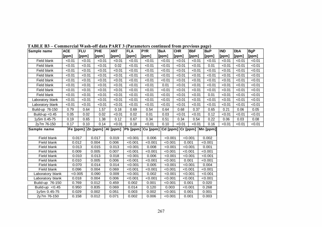
267
TABLE B3 – Commercial Wash-off data PART 3 (Parameters continued from previous page)
Field blank <0.01 <0.01 <0.01 <0.01 <0.01 <0.01 <0.01 <0.01 <0.01 <0.01 <0.01 <0.01 <0.01Field blank <0.01 <0.01 <0.01 0.02 <0.01 <0.01 <0.01 <0.01 <0.01 0.01 <0.01 <0.01 <0.01Field blank <0.01 <0.01 <0.01 <0.01 <0.01 <0.01 <0.01 <0.01 <0.01 <0.01 <0.01 <0.01 <0.01Field blank <0.01 <0.01 <0.01 <0.01 <0.01 <0.01 <0.01 <0.01 <0.01 <0.01 <0.01 <0.01 <0.01Field blank <0.01 <0.01 <0.01 <0.01 <0.01 <0.01 <0.01 <0.01 <0.01 <0.01 <0.01 <0.01 <0.01Field blank <0.01 <0.01 <0.01 <0.01 <0.01 <0.01 0.01 <0.01 <0.01 <0.01 <0.01 <0.01 <0.01Field blank <0.01 <0.01 <0.01 <0.01 <0.01 <0.01 <0.01 <0.01 <0.01 <0.01 <0.01 <0.01 <0.01Field blank <0.01 <0.01 <0.01 <0.01 <0.01 <0.01 <0.01 <0.01 <0.01 0.01 <0.01 <0.01 <0.01
Laboratory blank <0.01 <0.01 <0.01 <0.01 <0.01 <0.01 <0.01 <0.01 <0.01 <0.01 <0.01 <0.01 <0.01Laboratory blank <0.01 <0.01 <0.01 <0.01 <0.01 <0.01 <0.01 <0.01 <0.01 <0.01 <0.01 <0.01 <0.01Build-up 76-150 0.79 0.64 1.57 0.18 0.69 0.54 0.64 0.68 0.37 0.65 0.21 0.06 0.05Build-up <0.45 0.05 0.02 0.02 <0.01 0.02 0.01 0.03 <0.01 <0.01 0.12 <0.01 <0.01 <0.011y5m 0.45-75 0.19 0.65 1.38 0.12 0.67 0.34 0.51 0.34 0.54 0.22 0.06 0.03 0.08 2y7m 76-150 0.17 0.10 0.14 <0.01 0.18 <0.01 0.10 <0.01 <0.01 0.16 <0.01 <0.01 <0.01
BaP [ppm]
IND [ppm]
DbA [ppm]
BgP [ppm]
Sample name ACE [ppm]
FLU [ppm]
PHE [ppm]
CHR [ppm]
BbF [ppm]
ANT [ppm]
FLA [ppm]
PYR [ppm]
BaA [ppm]
Field blank 0.017 0.017 0.019 <0.001 0.006 <0.001 <0.001 0.002Field blank 0.012 0.004 0.006 <0.001 <0.001 <0.001 0.001 <0.001Field blank 0.013 0.015 0.013 <0.001 0.008 <0.001 <0.001 0.001Field blank 0.009 0.005 0.007 <0.001 <0.001 <0.001 <0.001 <0.001Field blank 0.010 0.013 0.018 <0.001 0.006 <0.001 <0.001 <0.001Field blank 0.010 0.005 0.006 <0.001 <0.001 <0.001 0.001 <0.001Field blank 0.070 0.014 0.014 <0.001 0.005 <0.001 <0.001 0.004Field blank 0.096 0.004 0.069 <0.001 <0.001 <0.001 <0.001 <0.001
Laboratory blank <0.005 0.090 0.009 <0.001 0.002 <0.001 <0.001 <0.001Laboratory blank 0.018 0.004 0.006 <0.001 <0.001 <0.001 <0.001 <0.001Build-up 76-150 0.769 0.012 0.459 0.002 0.001 <0.001 0.001 0.020Build-up <0.45 0.950 0.835 0.069 0.014 0.120 0.003 <0.001 0.2681y5m 0.45-75 0.029 0.002 0.051 0.003 0.002 <0.001 0.001 0.0012y7m 76-150 0.158 0.012 0.071 0.002 0.006 <0.001 0.001 0.003
Mn [ppm]Pb [ppm] Cu [ppm] Cd [ppm] Cr [ppm]Sample name Fe [ppm] Zn [ppm] Al [ppm]

268
TABLE B4 – Mean concentrations [mg/kg] of PAHs in the different particle size classes in wash-off samples at the residential site <0.45μm 0.45-75μm 76-150μm >150μm PAH DF [%] Mean SD DF [%] Mean SD DF [%] Mean SD DF [%] Mean SD
NAP 89 0.05 0.02 100 0.94 0.25 100 1.01 0.10 100 0.93 0.09 ACY 22 0.01 0.01 100 0.12 0.05 55 0.12 0.07 33 0.12 0.07 ACE 0 <0.01 <0.01 67 0.07 0.04 11 0.13 0.04 11 0.07 0.02 FLU 0 <0.01 <0.01 44 0.08 0.06 11 0.11 0.04 0 <0.01 <0.01 PHE 0 <0.01 <0.01 55 0.12 0.10 33 0.16 0.08 0 <0.01 <0.01 ANT 0 <0.01 <0.01 67 0.09 0.05 55 0.15 0.08 0 <0.01 <0.01 FLA 0 <0.01 <0.01 55 0.18 0.11 55 0.20 0.12 67 0.18 0.10 PYR 0 <0.01 <0.01 55 0.14 0.09 55 0.17 0.12 67 0.15 0.09 BaA 0 <0.01 <0.01 67 0.13 0.09 33 0.18 0.10 22 0.06 0.03
CHR 0 <0.01 <0.01 11 0.10 0.03 11 0.16 0.05 0 <0.01 <0.01
BbF* 0 <0.01 <0.01 33 0.12 0.06 0 <0.01 <0.01 11 0.12 0.04 BaP 11 0.01 0.01 78 0.11 0.07 44 0.17 0.10 33 0.13 0.08 IND 0 <0.01 <0.01 0 <0.01 <0.01 0 <0.01 <0.01 0 <0.01 <0.01
DbA 0 <0.01 <0.01 0 <0.01 <0.01 0 <0.01 <0.01 0 <0.01 <0.01
BgP 0 <0.01 <0.01 0 <0.01 <0.01 0 <0.01 <0.01 0 <0.01 <0.01 DF = Detection Frequency; SD = Standard deviation from mean;
* Benzo[b]flouranthene (BbF) and Benzo[k]flouranthene (BkF) was measured as one parameter

269
TABLE B5 – Mean concentrations [mg/kg] of PAHs in the different particle size classes in wash-off samples at the industrial site <0.45μm 0.45-75μm 76-150μm >150μm PAH DF [%] Mean SD DF [%] Mean SD DF [%] Mean SD DF [%] Mean SD
NAP 100 0.07 0.01 100 1.91 0.27 100 1.77 0.39 100 0.71 0.21 ACY 55 0.02 0.01 100 0.19 0.09 91 0.20 0.09 82 0.11 0.05 ACE 64 0.02 0.01 100 0.28 0.06 100 0.22 0.08 45 0.05 0.03 FLU 9 0.01 0.01 91 0.08 0.04 73 0.05 0.03 55 0.03 0.02 PHE 0 <0.01 <0.01 100 0.12 0.05 91 0.06 0.03 36 0.01 0.01 ANT 0 <0.01 <0.01 91 0.05 0.02 82 0.06 0.04 0 <0.01 <0.01 FLA 64 0.01 0.01 91 0.17 0.06 91 0.09 0.05 82 0.08 0.04 PYR 0 <0.01 <0.01 91 0.20 0.07 82 0.07 0.04 73 0.07 0.05 BaA 18 0.01 0.01 100 0.12 0.02 82 0.09 0.04 22 0.06 0.03
CHR 0 <0.01 <0.01 73 0.24 0.11 64 0.10 0.05 73 0.07 0.03
BbF* 0 <0.01 <0.01 82 0.07 0.03 82 0.04 0.02 45 0.02 0.01 BaP 27 0.04 0.03 100 0.11 0.03 100 0.07 0.03 73 0.08 0.04 IND 0 <0.01 <0.01 82 0.02 0.01 0 <0.01 <0.01 0 <0.01 <0.01
DbA 0 <0.01 <0.01 0 <0.01 <0.01 0 <0.01 <0.01 0 <0.01 <0.01
BgP 18 0.01 0.01 55 0.02 0.01 64 0.02 0.01 0 <0.01 <0.01 DF = Detection Frequency; SD = Standard deviation from mean;
* Benzo[b]flouranthene (BbF) and Benzo[k]flouranthene (BkF) was measured as one parameter

270
TABLE B6 – Mean concentrations [mg/kg] of PAHs in the different particle size classes in wash-off samples at the commercial site <0.45μm 0.45-75μm 76-150μm >150μm PAH DF [%] Mean SD DF [%] Mean SD DF [%] Mean SD DF [%] Mean SD
NAP 92 0.13 0.13 100 5.18 1.83 100 1.58 0.99 100 0.99 0.50 ACY 58 0.04 0.03 100 0.55 0.24 100 0.37 0.20 83 0.22 0.15 ACE 33 0.02 0.01 100 0.21 0.19 92 0.11 0.06 83 0.08 0.05 FLU 25 0.01 0.01 100 0.30 0.25 75 0.09 0.07 67 0.07 0.06 PHE 42 0.02 0.02 100 0.55 0.46 67 0.23 0.27 33 0.05 0.03 ANT 58 0.02 0.02 92 0.11 0.06 33 0.03 0.02 33 0.05 0.03 FLA 58 0.03 0.02 100 0.36 0.24 58 0.16 0.10 100 0.11 0.05 PYR 8 0.01 0.01 100 0.32 0.12 75 0.07 0.05 83 0.14 0.09 BaA 50 0.02 0.01 100 0.38 0.08 83 0.18 0.11 50 0.08 0.05
CHR 42 0.01 0.01 100 0.20 0.11 58 0.14 0.10 42 0.10 0.07
BbF* 8 0.01 0.01 100 0.39 0.14 67 0.14 0.08 58 0.09 0.06 BaP 75 0.06 0.06 100 0.26 0.10 83 0.13 0.09 83 0.09 0.06 IND 8 0.01 0.01 83 0.09 0.06 25 0.03 0.02 8 0.07 0.01
DbA 0 <0.01 <0.01 67 0.04 0.04 0 <0.01 <0.01 8 0.02 0.01
BgP 8 0.01 0.01 92 0.04 0.02 33 0.03 0.02 0 <0.01 <0.01 DF = Detection Frequency; SD = Standard deviation from mean;
* Benzo[b]flouranthene (BbF) and Benzo[k]flouranthene (BkF) was measured as one parameter

271
FIGURE B1 Particle size distribution graph for build-up sample taken at the
residential site
FIGURE B2 Particle size distribution graph for build-up sample taken at the
industrial site
Particle Diameter (µm.)
Volume (%)
0
10
0
10
20
30
40
50
60
70
80
90
100
0.01 0.1 1.0 10.0 100.0 1000.0
Particle Diameter (µm.)
%
0
10
0
10
20
30
40
50
60
70
80
90
100
0.01 0.1 1.0 10.0 100.0 1000.0
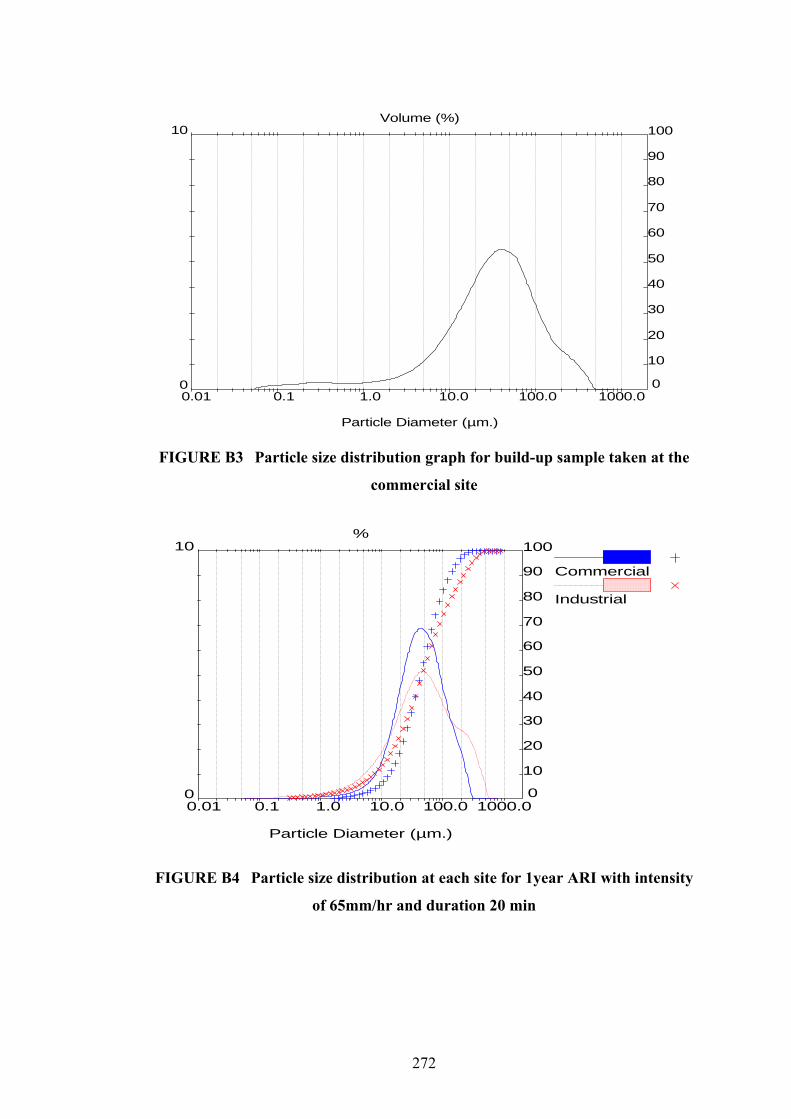
272
FIGURE B3 Particle size distribution graph for build-up sample taken at the
commercial site
Particle Diameter (µm.)
%
0
10
0
10
20
30
40
50
60
70
80
90
100
0.01 0.1 1.0 10.0 100.0 1000.0
Commercial
Industrial
FIGURE B4 Particle size distribution at each site for 1year ARI with intensity
of 65mm/hr and duration 20 min
Particle Diameter (µm.)
Volume (%)
0
10
0
10
20
30
40
50
60
70
80
90
100
0.01 0.1 1.0 10.0 100.0 1000.0

273
Particle Diameter (µm.)
%
0
10
0
10
20
30
40
50
60
70
80
90
100
0.01 0.1 1.0 10.0 100.0 1000.0
Industrial
Commercial
FIGURE B5 Particle size distribution at each site for 2year ARI with intensity
of 65mm/hr and duration 35 min
Particle Diameter (µm.)
%
0
10
0
10
20
30
40
50
60
70
80
90
100
0.01 0.1 1.0 10.0 100.0 1000.0
Commercial
Industrial
FIGURE B6 Particle size distribution at each site for 10year ARI with intensity
of 65mm/hr and duration 65 min

274
Particle Diameter (µm.)
%
0
10
0
10
20
30
40
50
60
70
80
90
100
0.01 0.1 1.0 10.0 100.0 1000.0
Industrial
Residential
Commercial
FIGURE B7 Particle size distribution at each site for 1year ARI with intensity
of 86mm/hr and duration 10 min
Particle Diameter (µm.)
%
0
10
0
10
20
30
40
50
60
70
80
90
100
0.01 0.1 1.0 10.0 100.0 1000.0
Commercial
Residential
Industrial
FIGURE B8 Particle size distribution at each site for 2year ARI with intensity
of 86mm/hr and duration 20 min

275
Particle Diameter (µm.)
%
0
10
0
10
20
30
40
50
60
70
80
90
100
0.01 0.1 1.0 10.0 100.0 1000.0
Industrial
Commercial
Residential
FIGURE B9 Particle size distribution at each site for 10year ARI with intensity
of 86mm/hr and duration 40 min
Particle Diameter (µm.)
%
0
10
0
10
20
30
40
50
60
70
80
90
100
0.01 0.1 1.0 10.0 100.0 1000.0
Residential
Commercial
Industrial
FIGURE B10 Particle size distribution at each site for 1year ARI with intensity
of 115mm/hr and duration 5 min

276
Particle Diameter (µm.)
%
0
10
0
10
20
30
40
50
60
70
80
90
100
0.01 0.1 1.0 10.0 100.0 1000.0
Industrial
Commercial
Residential
FIGURE B11 Particle size distribution at each site for 2year ARI with intensity
of 115mm/hr and duration 10 min
Particle Diameter (µm.)
%
0
10
0
10
20
30
40
50
60
70
80
90
100
0.01 0.1 1.0 10.0 100.0 1000.0
Residential
Commercial
FIGURE B12 Particle size distribution at each site for 10year ARI with intensity
of 115mm/hr and duration 25 min

277
Particle Diameter (µm.)
%
0
10
0
10
20
30
40
50
60
70
80
90
100
0.01 0.1 1.0 10.0 100.0 1000.0
Industrial
Commercial
Residential
FIGURE B13 Particle size distribution at each site for 2year ARI with intensity
of 133mm/hr and duration 7 min
Particle Diameter (µm.)
%
0
10
0
10
20
30
40
50
60
70
80
90
100
0.01 0.1 1.0 10.0 100.0 1000.0
Residential
Commercial
Industrial
FIGURE B14 Particle size distribution at each site for 5year ARI with intensity
of 133mm/hr and duration 13 min

278
Particle Diameter (µm.)
%
0
10
0
10
20
30
40
50
60
70
80
90
100
0.01 0.1 1.0 10.0 100.0 1000.0
Industrial
Commercial
Residential
FIGURE B15 Particle size distribution at each site for 10year ARI with intensity
of 133mm/hr and duration 17 min

279
APPENDIX C
CHEMOMETRIC ANALYSIS USING PCA

280
The method of principal component analysis (adapted from Jackson (1991))
The method of PCA is based on a key result from matrix algebra: A p x p symmetric,
non-singular matrix, such as the covariance matrix S, may be reduced to a diagonal
matrix L by premultiplying and postmultiplying it by a particular orthonormal matrix
U such that:
LSUU =′
The diagonal elements of L (l1, l2, ….lp) are called the eigenvalues of S. The columns
of U (u1, u2, …, up) are called the eigenvectors of S.
The starting point for PCA is the sample covariance matrix S. For a p-variable
problem,
⎥⎥⎥⎥⎥
⎦
⎤
⎢⎢⎢⎢⎢
⎣
⎡
=
221
22212
11221
.......
...
...
ppp
p
p
sss
ssssss
S
The principal axis transformation will transform p correlated variables (x1, x2, …, xp)
into p new uncorrelated variables (z1, z2, …, zp). The coordinate axes of these new
variables are described by the characteristic vectors ui which make up the matrix U
of direction cosines used in the transformation:
][ xxUz −′=
Where x and x are p x 1 vectors of observations on the original variables and their
means (loadings and scores). The transformed variables are called the principal
components of x of PCs for short. The ith principal component is
][ xxuz ii −′=
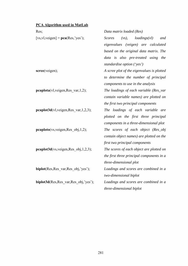
281
PCA Algorithm used in MatLab
Res; Data matrix loaded (Res)
[vs,vl,veigen] = pca(Res,’yes’); Scores (vs), loadings(vl) and
eigenvalues (veigen) are calculated
based on the original data matrix. The
data is also pre-treated using the
standardise option (‘yes’)
scree(veigen); A scree plot of the eigenvalues is plotted
to determine the number of principal
components to use in the analysis
pcaplota(vl,veigen,Res_var,1,2); The loadings of each variable (Res_var
contain variable names) are plotted on
the first two principal components
pcaplot3d(vl,veigen,Res_var,1,2,3); The loadings of each variable are
plotted on the first three principal
components in a three-dimensional plot
pcaploto(vs,veigen,Res_obj,1,2); The scores of each object (Res_obj
contain object names) are plotted on the
first two principal components
pcaplot3d(vs,veigen,Res_obj,1,2,3); The scores of each object are plotted on
the first three principal components in a
three-dimensional plot
biplot(Res,Res_var,Res_obj,’yes’); Loadings and scores are combined in a
two-dimensional biplot
biplot3d(Res,Res_var,Res_obj,’yes’); Loadings and scores are combined in a
three-dimensional biplot

282
The PCA function in MatLab (adapted from Kramer (1993))
function [vs, vl, veigen] = pca(x, standardise)
% [vs, vl, veigen] = PCA(x, standardise)
%
% This function performs principal component analysis using eigenvalue/
% eigenvector decomposition.
%
% returned are: the scores matrix, vs
% the loadings matrix, vl
% the normalised eigenvalues, veigen
%
% Standardise: 'none' = absent
% 'yes'
% 'no'
%
% A "standardise" option of "no" mean centers the x data but does not
% normalise to unit variance. Whereas the "yes" option mean centers and
% then normalises the x data to unit variance. When the "standardise"
% option is or omitted, then neither centering nor normalisation
% is carried out.
%
if nargin == 1
xc = x' * x;
elseif nargin == 2
[m, n] = size(x);
mx = mean(x);
if strcmp(standardise, 'yes')
xc = corrcoef(x);
% column centre and normalise to unit variance
sx = std(x);
for i=1:n
x(:,i) = (x(:,i) - mx(i))./sx(i);
end

283
elseif strcmp(standardise, 'no')
xc = cov(x);
% column centre
for i=1:n
x(:,i) = x(:,i) - mx(i);
end
elseif ~strcmp(standardise, 'none')
disp('Error: Invalid option specified')
end
else
disp('Error: Invalid number of input arguments')
end
[v, d] = eig(xc);
[veigen, order] = sort(diag(d)); % sort eigenvalues into ascending order
order = flipud(order); % we require principal components in descending order
veigen = flipud(veigen);
veigen = veigen./sum(veigen); % evals as fraction of total variance
vl = v(:, order); % arrange eigenvectors into same order as eigenvalues
vs = (vl' * x')'; % project eigenvalues to find scores

284
The Scree function in MatLab (adapted from Kramer (1993))
function [S] = scree(veigen)
% scree(veigen)
%
% Constructs a scree plot for the number of significant PC's from the output
% data of the PCA or SPCA functions.
%
% input: veigen is a matrix of eigenvectors returned from PCA or SPCA
%
% output: S is the vector containing the sum of the eigenvectors squared
%
[m,n] = size(veigen)
Z = veigen.^2
S = sum(Z)
plot(Z,'b-')
set(gca,'xtick',[1 2 3 4 5 6 7 8 9 10])
title('Scree Plot')
xlabel('Principal Component')
ylabel('Residual Variance, V')

285
The pcaplota function in MatLab (adapted from Kramer (1993))
function pcaplota(y, veigen, lbls, pc1, pc2)
% PCAPLOT(y, lbls, pc1, pc2)
%
% Constructs a plot from the output data of the PCA or SPCA functions. It
% can be used to create either a loadings vs loading plot or a scores vs
% scores plot.
%
% input: y is a loadings or scores matrix returned from PCA or SPCA
%
% lbls is: vector of strings containing text labels for the variables
% (columns)
%
% optional arguments (if these argument are omitted then a PC1 vs PC2
% plot is assumed:
%
% pc1 is the first principal component to plot
% pc2 is the second principal component to plot
%
[m, n]=size(y);
if (nargin == 3) % assume a PC1 vs PC2 plot is required
pc1 = 1;
pc2 = 2;
elseif (nargin ~= 5) % pc1 and pc2 contain PCs to plot
disp('Error: Incorrect number of input arguments')
end
plot(y(:,pc1), y(:,pc2), 'ro', 0, 0, 'b+') % include (0, 0) in plot
text(y(:,pc1), y(:,pc2), lbls) % annotate plot
for i=1:n
line([ 0 y(i,pc1)], [0 y(i,pc2)],'color', [1 0 0])
end

286
title('Principal Component Analysis')
str1 = ['PC1 (' num2str(veigen(1)*100,3) ' %)'];
str2 = ['PC2 (' num2str(veigen(2)*100,3) ' %)'];
xlabel(str1)
ylabel(str2)
k = axis; % find axis coordinates
% draw in axis lines to mark quadrants
line([k(1) k(2)], [0 0],'color',[0 0 1])
line([0 0], [k(3) k(4)],'color',[0 0 1])
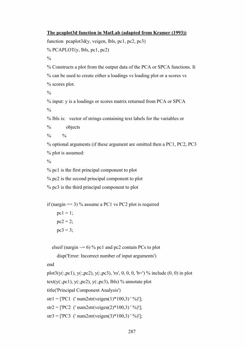
287
The pcaplot3d function in MatLab (adapted from Kramer (1993))
function pcaplot3d(y, veigen, lbls, pc1, pc2, pc3)
% PCAPLOT(y, lbls, pc1, pc2)
%
% Constructs a plot from the output data of the PCA or SPCA functions. It
% can be used to create either a loadings vs loading plot or a scores vs
% scores plot.
%
% input: y is a loadings or scores matrix returned from PCA or SPCA
%
% lbls is: vector of strings containing text labels for the variables or
% objects
% %
% optional arguments (if these argument are omitted then a PC1, PC2, PC3
% plot is assumed:
%
% pc1 is the first principal component to plot
% pc2 is the second principal component to plot
% pc3 is the third principal component to plot
if (nargin == 3) % assume a PC1 vs PC2 plot is required
pc1 = 1;
pc2 = 2;
pc3 = 3;
elseif (nargin ~= 6) % pc1 and pc2 contain PCs to plot
disp('Error: Incorrect number of input arguments')
end
plot3(y(:,pc1), y(:,pc2), y(:,pc3), 'ro', 0, 0, 0, 'b+') % include (0, 0) in plot
text(y(:,pc1), y(:,pc2), y(:,pc3), lbls) % annotate plot
title('Principal Component Analysis')
str1 = ['PC1 (' num2str(veigen(1)*100,3) ' %)'];
str2 = ['PC2 (' num2str(veigen(2)*100,3) ' %)'];
str3 = ['PC3 (' num2str(veigen(3)*100,3) ' %)'];

288
xlabel(str1)
ylabel(str2)
zlabel(str3)
v = axis; % find axis coordinates
% draw in axis lines to mark quadrants
line([v(1) v(2)], [0 0], [0 0])
line([0 0], [v(3) v(4)], [0 0])
line([0 0], [0 0], [v(5) v(6)])
%Turn grid on
Grid on

289
The pcaploto function in MatLab (adapted from Kramer (1993))
function pcaploto(y, veigen, lbls, pc1, pc2)
% PCAPLOTo(y, lbls, pc1, pc2)
%
% Constructs a plot from the output data of the PCA or SPCA functions. It
% can be used to create either a loadings vs loading plot or a scores vs
% scores plot.
%
% input: y is a loadings or scores matrix returned from PCA or SPCA
%
% lbls is: vector of strings containing text labels for the variables
% (columns)
%
% optional arguments (if these argument are omitted then a PC1 vs PC2
% plot is assumed:
%
% pc1 is the first principal component to plot
% pc2 is the second principal component to plot
%
if (nargin == 3) % assume a PC1 vs PC2 plot is required
pc1 = 1;
pc2 = 2;
elseif (nargin ~= 5) % pc1 and pc2 contain PCs to plot
disp('Error: Incorrect number of input arguments')
end
plot(y(:,pc1), y(:,pc2), 'ro', 0, 0, 'b+') % include (0, 0) in plot
text(y(:,pc1), y(:,pc2), lbls) % annotate plot
title('Principal Component Analysis')
str1 = ['PC1 (' num2str(veigen(1)*100,3) ' %)'];
str2 = ['PC2 (' num2str(veigen(2)*100,3) ' %)'];
xlabel(str1)
ylabel(str2)
v = axis; % find axis coordinates

290
% draw in axis lines to mark quadrants
line([v(1) v(2)], [0 0],'color',[0 0 1])
line([0 0], [v(3) v(4)],'color',[0 0 1])

291
The biplot function in MatLab (adapted from Kramer (1993))
function biplot(x, lblsv, lblso, standardise)
% BIPLOT(x, lbls, standardise)
%
% Constructs a biplot from the input matrix x for principal component
% analysis using singular value decomposition algorithm.
%
% input: x is a (nxp) data matrix whose columns represent variables and
% whose rows represent samples (or observations).
%
% lblsv is: vector of strings containing text labels for the variables
% (columns)
% lblso is: vector of strings containing text labels for the objects
% (columns)
%
%
% Standardise is one of: 'none'
% 'yes'
% 'no'
%
% A "standardise" option of "no" mean centers the x data but does not
% standardise to unit variance. Whereas the "yes" option mean centers (by
% removing the mean from each column) and then standardises the x data to unit
% variance. When "none" is specified, then neither centering nor
% standardisation is carried out.
%
if (nargin == 4)
[m ,n] = size(x);
mx = mean(x);
if strcmp(standardise, 'yes')
% column centre and normalise to unit variance
sx = std(x);
for i=1:n
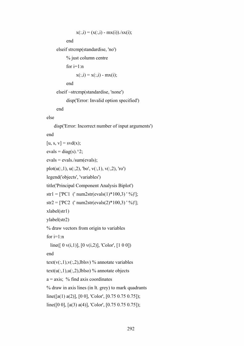
292
x(:,i) = (x(:,i) - mx(i))./sx(i);
end
elseif strcmp(standardise, 'no')
% just column centre
for i=1:n
x(:,i) = x(:,i) - mx(i);
end
elseif ~strcmp(standardise, 'none')
disp('Error: Invalid option specified')
end
else
disp('Error: Incorrect number of input arguments')
end
[u, s, v] = svd(x);
evals = diag(s).^2;
evals = evals./sum(evals);
plot(u(:,1), u(:,2), 'bo', v(:,1), v(:,2), 'ro')
legend('objects', 'variables')
title('Principal Component Analysis Biplot')
str1 = ['PC1 (' num2str(evals(1)*100,3) ' %)'];
str2 = ['PC2 (' num2str(evals(2)*100,3) ' %)'];
xlabel(str1)
ylabel(str2)
% draw vectors from origin to variables
for i=1:n
line([ 0 v(i,1)], [0 v(i,2)], 'Color', [1 0 0])
end
text(v(:,1),v(:,2),lblsv) % annotate variables
text(u(:,1),u(:,2),lblso) % annotate objects
a = axis; % find axis coordinates
% draw in axis lines (in lt. grey) to mark quadrants
line([a(1) a(2)], [0 0], 'Color', [0.75 0.75 0.75]);
line([0 0], [a(3) a(4)], 'Color', [0.75 0.75 0.75]);

293
The biplot3d function in MatLab (adapted from Kramer (1993))
function biplot3d(x, lblsv, lblso, standardise)
% BIPLOT(x, lbls, standardise)
%
% Constructs a biplot from the input matrix x for principal component
% analysis using singular value decomposition algorithm.
%
% input: x is a (nxp) data matrix whose columns represent variables and
% whose rows represent samples (or observations).
%
% lblsv is: vector of strings containing text labels for the variables
% (columns)
% lblso is: vector of strings containing text labels for the objects
% (columns)
%
%
% Standardise is one of: 'none'
% 'yes'
% 'no'
%
% A "standardise" option of "no" mean centers the x data but does not
% standardise to unit variance. Whereas the "yes" option mean centers (by
% removing the mean from each column) and then standardises the x data to unit
% variance. When "none" is specified, then neither centering nor
% standardisation is carried out.
%
if (nargin == 4)
[m ,n] = size(x);
mx = mean(x);
if strcmp(standardise, 'yes')
% column centre and normalise to unit variance
sx = std(x);
for i=1:n
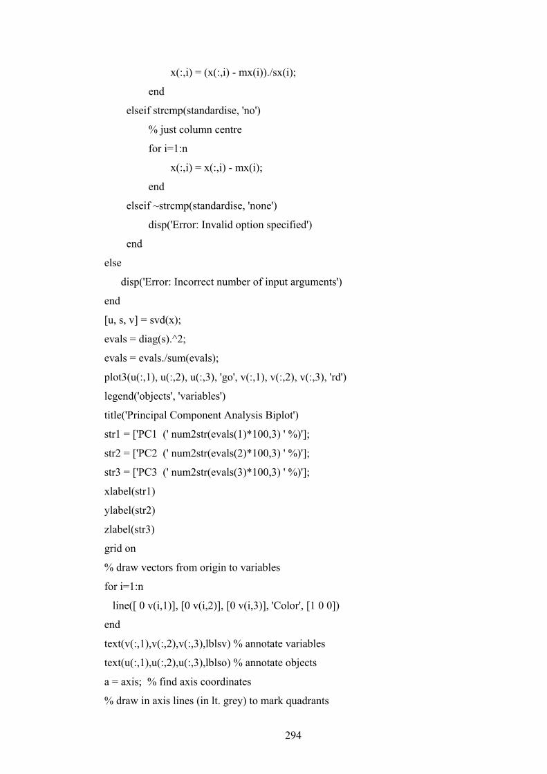
294
x(:,i) = (x(:,i) - mx(i))./sx(i);
end
elseif strcmp(standardise, 'no')
% just column centre
for i=1:n
x(:,i) = x(:,i) - mx(i);
end
elseif ~strcmp(standardise, 'none')
disp('Error: Invalid option specified')
end
else
disp('Error: Incorrect number of input arguments')
end
[u, s, v] = svd(x);
evals = diag(s).^2;
evals = evals./sum(evals);
plot3(u(:,1), u(:,2), u(:,3), 'go', v(:,1), v(:,2), v(:,3), 'rd')
legend('objects', 'variables')
title('Principal Component Analysis Biplot')
str1 = ['PC1 (' num2str(evals(1)*100,3) ' %)'];
str2 = ['PC2 (' num2str(evals(2)*100,3) ' %)'];
str3 = ['PC3 (' num2str(evals(3)*100,3) ' %)'];
xlabel(str1)
ylabel(str2)
zlabel(str3)
grid on
% draw vectors from origin to variables
for i=1:n
line([ 0 v(i,1)], [0 v(i,2)], [0 v(i,3)], 'Color', [1 0 0])
end
text(v(:,1),v(:,2),v(:,3),lblsv) % annotate variables
text(u(:,1),u(:,2),u(:,3),lblso) % annotate objects
a = axis; % find axis coordinates
% draw in axis lines (in lt. grey) to mark quadrants

295
line([a(1) a(2)], [0 0], [0 0], 'Color', [0 0 1])
line([0 0], [a(3) a(4)], [0 0], 'Color', [0 0 1])
line([0 0], [0 0], [a(5) a(6)], 'Color', [0 0 1])
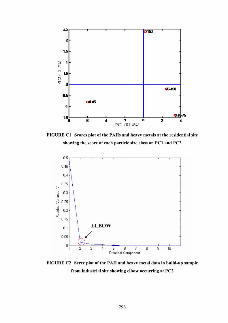
296
FIGURE C1 Scores plot of the PAHs and heavy metals at the residential site
showing the score of each particle size class on PC1 and PC2
FIGURE C2 Scree plot of the PAH and heavy metal data in build-up sample
from industrial site showing elbow occurring at PC2
ELBOW
PC1 (81.4%)
PC2
(12.
7%)

297
FIGURE C3 Scores plot of the PAHs and heavy metals at the industrial site
showing the score of each particle size class on PC1 and PC2
FIGURE C4 Scree plot of the PAH and heavy metal data in build-up sample
from commercial site showing elbow occurring at PC2
ELBOW
PC1 (73.4%)
PC2
(18.
5%)

298
FIGURE C5 Scores plot of the PAHs and heavy metals at the commercial site
showing the score of each particle size class on PC1 and PC2
FIGURE C6 Scree plot of dissolved data at the residential site indicating elbow
occurring at PC3
ELBOW
PC1 (73.4%)
PC2
(18.
5%)

299
FIGURE C7 Three dimensional loadings plot of the PAHs and heavy metals
detected in the dissolved fraction of wash-off samples from the residential site
1y10 = 1 year 10 minutes ARI event
FIGURE C8 Scores of each rainfall event on PC1 and PC2 at the residential
site when using PCA on detected PAHs and heavy metals in the dissolved
fraction

300
FIGURE C9 Scree plot of the PAHs and heavy metals (0.45-75μm) at the
residential site (elbow occurring at PC3)
FIGURE C10 Three dimensional loadings plot of the PAHs and heavy metals
detected in washed-off particles 0.45-75µm from the residential site
ELBOW
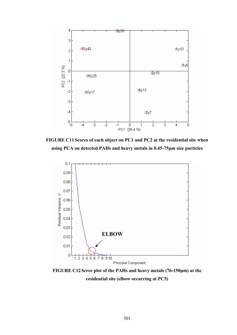
301
FIGURE C11 Scores of each object on PC1 and PC2 at the residential site when
using PCA on detected PAHs and heavy metals in 0.45-75μm size particles
FIGURE C12 Scree plot of the PAHs and heavy metals (76-150μm) at the
residential site (elbow occurring at PC5)
ELBOW
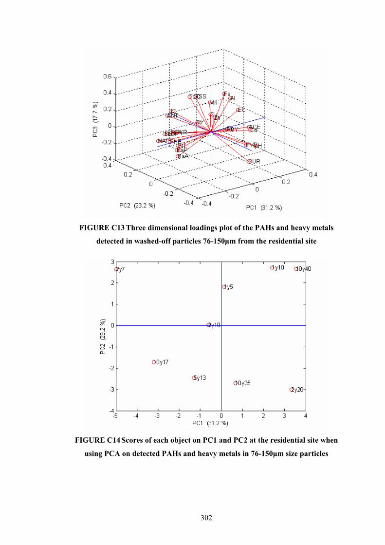
302
FIGURE C13 Three dimensional loadings plot of the PAHs and heavy metals
detected in washed-off particles 76-150µm from the residential site
FIGURE C14 Scores of each object on PC1 and PC2 at the residential site when
using PCA on detected PAHs and heavy metals in 76-150μm size particles

303
FIGURE C15 Scree plot of the PAHs and heavy metals (>150μm) at the
residential site (elbow occurring at PC3)
FIGURE C16 Three dimensional loadings plot of the PAHs and heavy metals
detected in washed-off particles >150µm from the residential site
ELBOW

304
FIGURE C17 Scores of each object on PC1 and PC2 at the residential site when
using PCA on detected PAHs and heavy metals in >150μm size particles
FIGURE C18 Scree plot of dissolved data at the industrial site indicating elbow
occurring at PC3
ELBOW

305
FIGURE C19 Three dimensional loadings plot of the PAHs and heavy metals
detected in dissolved samples from the industrial site
FIGURE C20 Scores of each rainfall event on PC1 and PC2 at the industrial site
when using PCA on detected PAHs and heavy metals in the dissolved fraction

306
FIGURE C21 Scree plot of the PAHs and heavy metals (0.45-75μm) at the
industrial site (elbow occurring at PC2)
FIGURE C22 Scores of each rainfall event on PC1 and PC2 at the industrial site
when using PCA on detected PAHs and heavy metals in particles 0.45-75µm
ELBOW
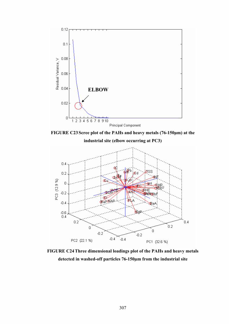
307
FIGURE C23 Scree plot of the PAHs and heavy metals (76-150μm) at the
industrial site (elbow occurring at PC3)
FIGURE C24 Three dimensional loadings plot of the PAHs and heavy metals
detected in washed-off particles 76-150µm from the industrial site
ELBOW

308
FIGURE C25 Scores of each rainfall event on PC1 and PC2 at the industrial site
when using PCA on detected PAHs and heavy metals in particles 76-150µm
FIGURE C26 Scree plot of the PAHs and heavy metals (>150μm) at the
industrial site (elbow occurring at PC2)
ELBOW
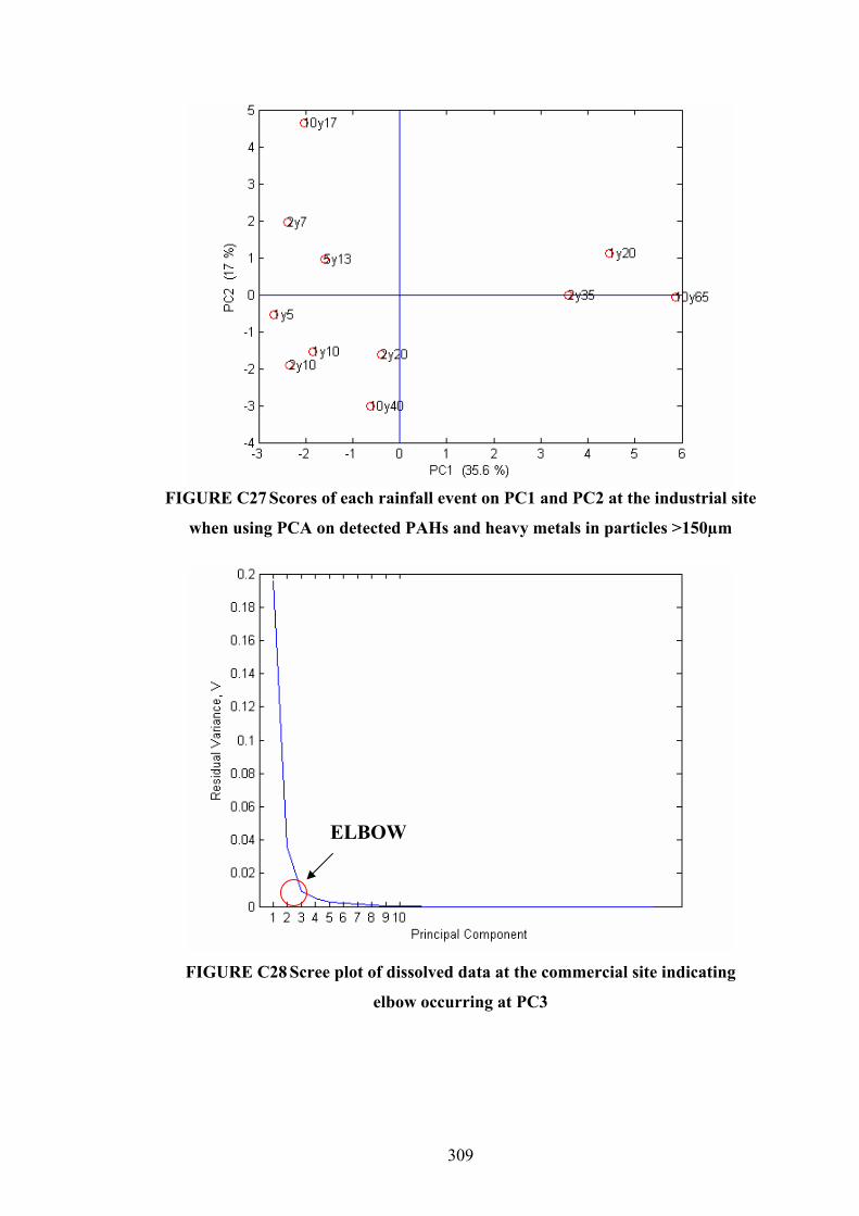
309
FIGURE C27 Scores of each rainfall event on PC1 and PC2 at the industrial site
when using PCA on detected PAHs and heavy metals in particles >150µm
FIGURE C28 Scree plot of dissolved data at the commercial site indicating
elbow occurring at PC3
ELBOW

310
FIGURE C29 Three dimensional loadings plot of the PAHs and heavy metals
detected in dissolved samples from the commercial site
FIGURE C30 Scores of each rainfall event on PC1 and PC2 at the commercial
site when using PCA on detected PAHs and heavy metals in the dissolved
fraction

311
FIGURE C31 Scree plot of the PAHs and heavy metals (0.45-75µm) at the
commercial site (elbow occurring at PC3)
FIGURE C32 Scores of each rainfall event on PC1 and PC2 at the commercial
site when using PCA on detected PAHs and heavy metals in particles 0.45-75µm
ELBOW

312
FIGURE C33 Scree plot of the PAHs and heavy metals (76-150µm) at the
commercial site (elbow occurring at PC4)
FIGURE C34 Three dimensional loadings plot of the PAHs and heavy metals
detected in washed-off particles 76-150µm from the commercial site
ELBOW

313
FIGURE C35 Scores of each rainfall event on PC1 and PC2 at the commercial
site when using PCA on detected PAHs and heavy metals in particles 76-150µm
FIGURE C36 Scree plot of the PAHs and heavy metals (76-150µm) at the
commercial site (elbow occurring at PC4)
ELBOW
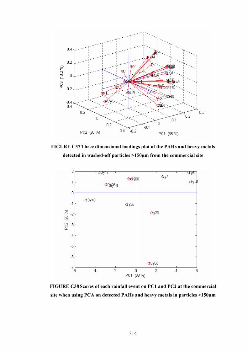
314
FIGURE C37 Three dimensional loadings plot of the PAHs and heavy metals
detected in washed-off particles >150µm from the commercial site
FIGURE C38 Scores of each rainfall event on PC1 and PC2 at the commercial
site when using PCA on detected PAHs and heavy metals in particles >150µm

315
APPENDIX D
PREDICTION USING PLS

316
PLS and the underlying scientific model (adapted from Wold et al. 2001))
The PLS model is developed from a training set of N observations (objects, cases,
compounds, process time points) with K X variables denoted by xk (k = 1, …, K),
and M Y-variables ym (m = 1, 2 ,…M). These training data form the two matrices X
and Y of dimensions (N x K) and (N x M), respectively.
The PLS model finds a few ‘new’ variables, which are estimates of the latent
variables or their rotations. These new variables are called X-scores and denoted by
ta (a = 1, 2, …, A). The X-scores are predictors of Y. The X-scores are few (A in
number), and orthogonal. They are estimated as linear combinations of the original
variables xk with the coefficients, ‘weights’, wka (a = 1, 2, …, A).
∑= k ikkaia XWt ; (T = XW).
The X-scores (ta’s) have the following properties:
a) They are, multiplied by the loadings pak, good summaries of X, so that the X
residuals, eik, are small:
With multivariate Y (when M>1) the corresponding Y-scores (ua) are, multiplied
with the weights cam, good summaries of Y, so that the residuals, gim, are small:
b) the X-scores are good predictors of Y:

317
PLS1 algorithm used in the research
1. Load Data and pretreat
Wash_off;
[Xcent,xmean] = pretreat(Wash_off);
[Wash_off2,xsdev] = varscale(Xcent);
2. Remove unwanted variables
Wash_off3 = Wash_off2(:,2:6);
3. Split into X and Y matrices (X predictors, Y to be predicted)
Y = Wash_off3(:, 4); Note: If using calibration/validation, split
e = [1;2;3;5]; appropriately
X = Wash_off3(:,e);
4. Run PLS Algorithm
[p, q, w, b, t, u, x, y] = pls1(X, Y); (p = X loadings; q = Y loadings; w = weights;
b = inner relationships; t = X scores;
u = Y scores; x = X residuals; y = Y residuals
5. Run NPLS Algorithm to see error predictions
[rev, secv, press] = npls(X, Y, x, y, p, q, w, b); NOTE: Use X, Y for x,y if no
validation data, else use
validation x,y (in this case ½ of
the data matrix was used for
validation)
Select appropriate n (# of factors) to use in prediction

318
6. Run REGEN algorithm to regenerate data using specified # of factors n
[Xr, Xresid] = regen(X', p, 2); NOTE: Transpose X data matrix as
calculates row-wise
7. Transpose Xr and Xresid to make calculate Column-wise
Xr=Xr'; Xresid=Xresid';
8. Run PLS1 prediction algorithm with selected # of factors
[pred, resp] = pls1pred(Xr, p, q, w, b, 2);
9. Run Observed vs Predicted plot algorithm
opplot(pred,Y,2,1,0,0,1); Note: Leave last 4 numerals as is -these
refer to alternative plotting options
10. Run Predicted error algorithm to obtain errors of fit
[SSE, SSF, SSX, SSY, R2X, R2Y, Q2, RMSEP] = SEP(Xr, Y, Xresid, y, press', pred, 2);

319
pretreat function used in MatLab (adapted from Mathisen (2004)) function [A, m, v] = pretreat(a)
%MEANCENT mean centers the data in a column-wise matrix
% [X, m] = MEANCENT(A)
%
% where:
%
% A is the mean centered data
% m is a vector containing the means
% xvar is a vector containing the variances
% data is the absorbance or concentration matrix
%
% MEANCENT expects the data to be organized column-wise per the MLR
conventions.
% The mean centering is performed row by row.
% If your data is organized row-wise per the PLS conventions, use the transpose
% of A, A' as the argument to MEANCENT.
[i, j] = size(a);
if j < 2,
error('Cannot scale the variance of less than 2 variables');
end
m = mean(a')';
x = a - m * ones(1,j);
xbar = mean(a')';
a = a - xbar * ones(1,j);
v = sqrt(sum(a' .* a'))';
A = a ./ (v * ones(1,j));

320
varscale function used in MatLab (adapted from Mathisen (2004))
function [x, xvar] = varscale(a)
%VARSCALE scales variance of the data in a matrix to equal Variables / (Points - 1)
% [x, xvar] = varscale(a)
%
% where:
%
% x is the scaled data
% xvar is a vector containing the variances
% a is the data matrix to be scaled
%
% VARSCALE expects the data to be organized column-wise per the MLR
conventions.
% The variance scaling is performed row by row.
% The mean of the data is removed prior to scaling and restored after scaling.
% The resulting data is NOT mean-centered. The total variance in the resulting
% data will be equal to Number of Variables / (Number of Points - 1).
%
% If your data is organized row-wise per the PLS conventions, use the transpose
% of A, A' as the argument of VARSCALE.
[i, j] = size(a);
if j < 2,
error('Cannot scale the variance of less than 2 variables');
end
xbar = mean(a')';
a = a - xbar * ones(1,j);
xvar = sqrt(sum(a' .* a'))';
x = a ./ (xvar * ones(1,j));
x = x + xbar * ones(1,j);

321
pls1 function used in MatLab (adapted from Mathisen (2004))
function [p, q, w, b, t, u, x, y] = pls1(a, c, maxrank)
%PLS1 Partial Least Squares in latent variables
% Uses the Matlab's SVD routine on the smallest covariance matrix
% for computational efficiency. This function individually computes the
% PLS calibration each component (column) in the C matrix even if the C
% matrix contains more than one component (column). If you wish to calculate
% a PLS calibration using all component information simultaneously, then
% you should use the function PLS. Conforms to ASTM standard E 1655-97.
%
% [P, Q, W, B] = PLS1(A, C, MAXRANK) or,
%
% [P, Q, W, B, T, U, X, Y] = PLS1(A, C, MAXRANK)
%
% Where:
%
% P is the matrix of spectral factors
% Q is the matrix of concentration factors
% W is the matrix of weights
% B is the vector containing the inner relationships
% T is the matrix of spectral scores
% U is the matrix of concentration scores
% X is the matrix of spectral residuals
% Y is the matrix of concentration residuals
% A is the training set absorbance matrix
% C is the training set concentration matrix
% MAXRANK is optional limit to the number of factors calculated
[m,n] = size(a);
[m,l] = size(c);
if l ~= 1,
message=[ num2str(l), ' C variables. PLS1 requires a single variable in the C
matrix.'];
error(message);

322
end
if nargin == 3, i = min([n, m, maxrank]); else i = min([n m]); end
x = a;
y = c;
for h = 1:i,
w(:,h) = x' * y;
w(:,h) = w(:,h) / sqrt(w(:,h)' * w(:,h));
t(:,h) = x * w(:,h);
tsq = t(:,h)' * t(:,h);
p(:,h) = ( x' * t(:,h) ) / tsq;
q(:,h) = ( y' * t(:,h) ) / tsq;
u(:,h) = y * q(:,h);
x = x - (t(:,h) * p(:,h)');
y = y - (t(:,h) * q(:,h)');
end
b=ones(1,i);

323
npls function used in MatLab (adapted from Mathisen (2004))
function [rev, secv, press] = npls(X, Y, xv, yv, p, q, w, b)
rev = plsrev(X, p, q, w, b);
secv = plscross(X, Y);
press = plspress(xv, yv, p, q, w, b);
plot(rev);
title('Reduced Eigenvalues')
xlabel('Number of PCs')
ylabel('REV')
figure
plot(secv);
title('Standard Error of Cross-Validation')
xlabel('Number of PCs')
ylabel('SECV')
figure
plot(press);
title('Predicted Residual Error Sum of Squares')
xlabel('Number of PCs')
ylabel('PRESS')

324
regen function used in MatLab (adapted from Mathisen (2004))
function [reg, resid] = regen(a, vc, r)
%REGEN PCA short cicuit data reproduction using N factors.
% REG = REGEN(A, VC, R) or [REG, RESID] = REGEN(A, VC, R)
%
% Where:
%
% REG is the matrix containing the regenerated data
% RESID is the matrix containing the residuals of the regeneration
% A is the absorbance matrix
% VC is the matrix containing the factors
% R is the rank (number of factors) to use in the regeneration
[t, n] = size(vc);
if nargin == 3, n = min([n, r]);, end;
vc = vc(:, 1:n);
reg = (a' * vc * vc')';
resid = a - reg;

325
pls1pred function used in MatLab (adapted from Mathisen (2004))
function [c, x] = pls1pred(a, p, q, w, b, n, amean, cmean, ascal, cscal)
%PLS1PRED Predicts unknown concentrations using PLS1.
%
% [C, X] = PLS1PRED(A, P, Q, W, B, N, AMEAN, CMEAN, ASCAL,
CSCAL)
%
% C is the matrix of the unknown's concentrations
% X is the matrix of spectral residuals after decomposition
% A is the unknown spectrum (or spectra)
% P is the matrix of spectral factors
% Q is the matrix of concentration factors
% W is the matrix of weights
% B is the vector containing the inner relationships
% if B == 0, then all b's are set to unity
% N is the number of factors to use
%
% optional arguments:
%
% AMEAN vector of means of mean-centered calibration spectra
% CMEAN vector of means of mean-centered calibration concentrations
% ASCAL vector of scaling factors of scaled calibration spectra
% CSCAL vector of scaling factors of scaled calibration concentrations
%
% Specify 0 for amean, cmean, ascal, cscal if no scaling or centering
[maxrank, h] = size(p);
if nargin > 5, maxrank = min([n, maxrank]); end
if sum(size(b)==1) == 2,
if b==0,
b=ones(1,maxrank);
end
end

326
c=0;
[j, i] = size(a);
if nargin > 6,
if amean ~= 0,
a = a - amean * ones(1, j);
end
if nargin > 8,
if ascal ~= 0,
a = a ./ (ascal * ones(1, j));
end
end
end
x = a;
for h=1:maxrank
t(:,h) = x * w(:,h);
x = x - t(:,h) * p(:,h)';
c = c + b(h) * t(:,h) * q(:,h);
end
[l, k] = size(c);
if nargin > 9,
if cscal ~= 0
c = c .* (cscal * ones(1,l));
end
end
if nargin > 7,
if cmean ~=0,
c = c + cmean * ones(1,l);
end
end

327
opplot function used in MatLab (adapted from Mathisen (2004))
function opplot(pred,meas,lv,num,rmse,rmsestr,st)
%MVPMPLOT -- predicted vs. measured plot
%mvpmplot(pred,meas,lv,num,rmse,rmsestr,st)
%Inputs: pred predicted values
% meas measured values
% lv number of latent variables (optional)
% num if > 0, plot with numbers
% rmse root mean square error of [cal,crossval,pred] (optional)
% rmsestr root mean square error text string (optional)
% st if zero (0), omit statistics
% Description:
% This function creates a predicted/measured plot, with some
% statistics and a regression line.
%
[m,n] = size(pred); [p,q] = size(meas);
if max(m,n) ~= max(p,q), error('vectors must have same size!')
end
if min(m,n) ~= 1 | min(p,q) ~= 1,
error('input must be vectors!')
end
% select plot character depending of number of objects
if length(meas) > 75,
plotchar = '.b';
else plotchar = 'ob';
end
% plot max and min
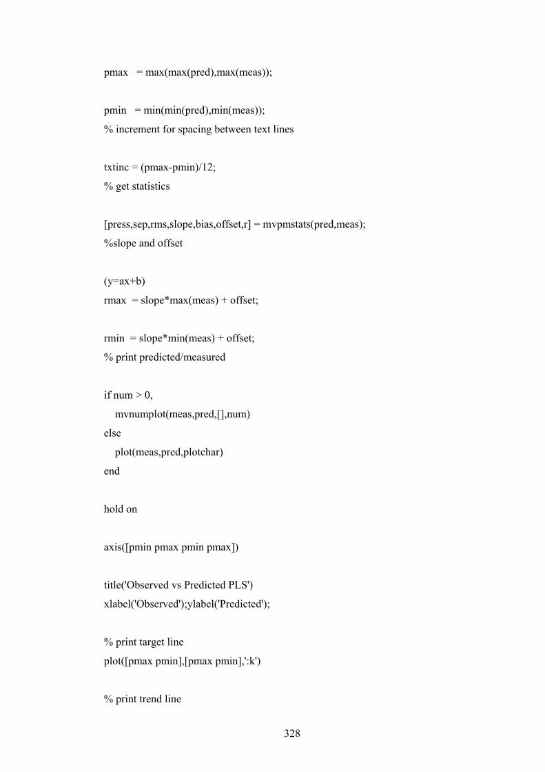
328
pmax = max(max(pred),max(meas));
pmin = min(min(pred),min(meas));
% increment for spacing between text lines
txtinc = (pmax-pmin)/12;
% get statistics
[press,sep,rms,slope,bias,offset,r] = mvpmstats(pred,meas);
%slope and offset
(y=ax+b)
rmax = slope*max(meas) + offset;
rmin = slope*min(meas) + offset;
% print predicted/measured
if num > 0,
mvnumplot(meas,pred,[],num)
else
plot(meas,pred,plotchar)
end
hold on
axis([pmin pmax pmin pmax])
title('Observed vs Predicted PLS')
xlabel('Observed');ylabel('Predicted');
% print target line
plot([pmax pmin],[pmax pmin],':k')
% print trend line

329
plot([pmax pmin],[rmax rmin],'--m')
if exist('st') == 0 | st ~= 0,
% print statistics
txt1=text(pmin+txtinc,pmax-1/2*txtinc,['Objects: ' num2str(max(m,n))]);
txt2=text(pmin+txtinc,pmax-2/2*txtinc,['Slope: ' num2str(slope)]);
txt3=text(pmin+txtinc,pmax-3/2*txtinc,['Offset: ' num2str(offset)]);
txt4=text(pmin+txtinc,pmax-4/2*txtinc,['Bias: ' num2str(bias)]);
txt5=text(pmin+txtinc,pmax-5/2*txtinc,['Correlation: ' num2str(r)]);
txt6=text(pmin+txtinc,pmax-6/2*txtinc,['SEP: ' num2str(sep)]);
if exist('rmse'), if ~exist ('rmsestr'), rmsestr = 'RMSEP';
end
txt7=text(pmin+txtinc,pmax-7/2*txtinc,[rmsestr ': ' num2str(rmse)]);
else
txt7=text(pmin+txtinc,pmax-7/2*txtinc,['RMSEP: ' num2str(rmsep)]);
end
if exist('lv'),
txt8=text(pmin+txtinc,pmax-8/2*txtinc,['Latent var.: ' int2str(lv)]);
end
for i = 1:8, set(eval(['txt' int2str(i)]),'FontSize',8);
end
end
end of mvpmplot

330
SEP function used in MatLab (adapted from Mathisen (2004))
function [SSE, SSF, SSX, SSY, R2X, R2Y, Q2, RMSEP] = SEP(X, Y, x, y, press,
pred, n)
SSE = sum(x.^2);
SSF = sum(y.^2);
SSX = sum(X.^2);
SSY = sum(Y.^2);
P = sum(press.^2);
R2X = (1-(SSE/SSX))*100;
R2Y = (1-(SSF/SSY))*100;
Q2 = (1-(P/SSY))*100;
RMSEP = (sum(((pred-Y).^2)/n)).^0.5;

331
TABLE D1 Abbreviations of objects in Matrix A
Abbreviation Real name (Site, ARI event, particle size)
1 Residential Build-up >300µm
2 Residential Build-up 151-300µm
3 Residential Build-up 76-150µm
4 Residential Build-up 0.45-75µm
5 Residential Build-up <0.45µm
6 Residential 1y10min >300µm
7 Residential 1y10min 151-300µm
8 Residential 1y10min 76-150µm
9 Residential 1y10min 0.45-75µm
10 Residential 1y10min <0.45µm
11 Residential 2y20min >300µm
12 Residential 2y20min 151-300µm
13 Residential 2y20min 76-150µm
14 Residential 2y20min 0.45-75µm
15 Residential 2y20min <0.45µm
16 Residential 10y40min >300µm
17 Residential 10y40min 151-300µm
18 Residential 10y40min 76-150µm
19 Residential 10y40min 0.45-75µm
20 Residential 10y40min <0.45µm
21 Residential 1y5min >300µm
22 Residential 1y5min 151-300µm
23 Residential 1y5min 76-150µm
24 Residential 1y5min 0.45-75µm
25 Residential 1y5min <0.45µm
26 Residential 2y10min >300µm
27 Residential 2y10min 151-300µm
28 Residential 2y10min 76-150µm
29 Residential 2y10min 0.45-75µm
30 Residential 2y10min <0.45µm
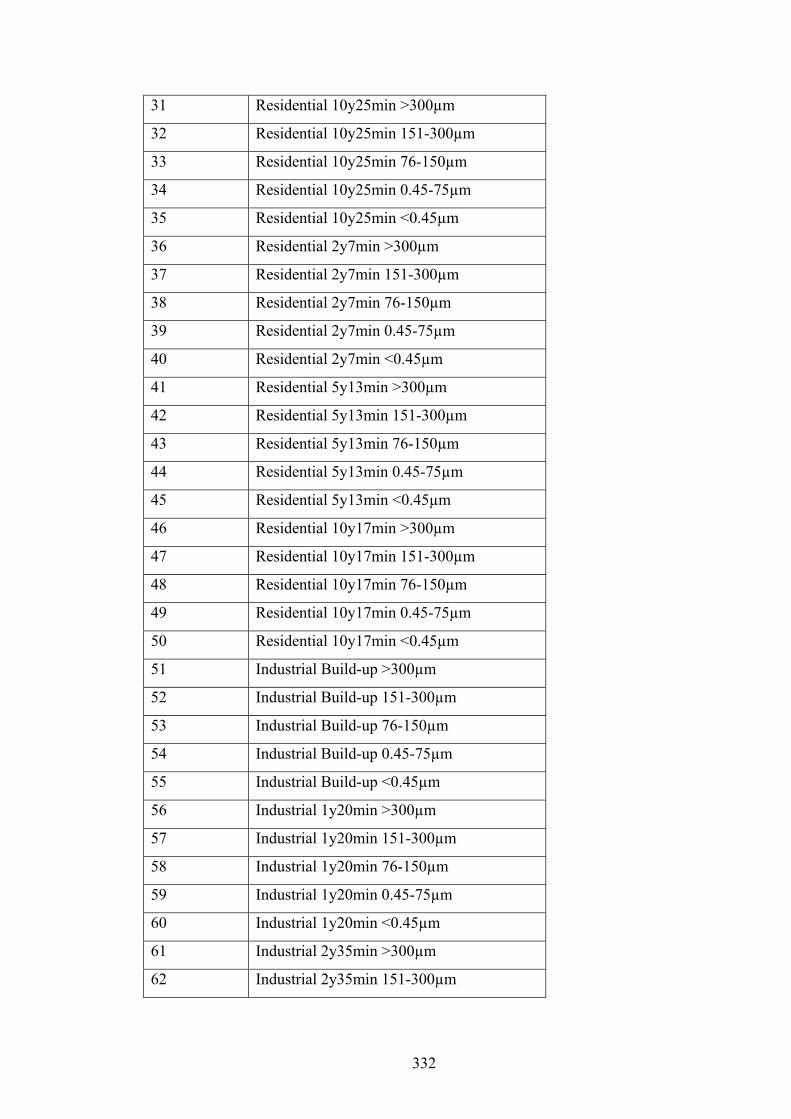
332
31 Residential 10y25min >300µm
32 Residential 10y25min 151-300µm
33 Residential 10y25min 76-150µm
34 Residential 10y25min 0.45-75µm
35 Residential 10y25min <0.45µm
36 Residential 2y7min >300µm
37 Residential 2y7min 151-300µm
38 Residential 2y7min 76-150µm
39 Residential 2y7min 0.45-75µm
40 Residential 2y7min <0.45µm
41 Residential 5y13min >300µm
42 Residential 5y13min 151-300µm
43 Residential 5y13min 76-150µm
44 Residential 5y13min 0.45-75µm
45 Residential 5y13min <0.45µm
46 Residential 10y17min >300µm
47 Residential 10y17min 151-300µm
48 Residential 10y17min 76-150µm
49 Residential 10y17min 0.45-75µm
50 Residential 10y17min <0.45µm
51 Industrial Build-up >300µm
52 Industrial Build-up 151-300µm
53 Industrial Build-up 76-150µm
54 Industrial Build-up 0.45-75µm
55 Industrial Build-up <0.45µm
56 Industrial 1y20min >300µm
57 Industrial 1y20min 151-300µm
58 Industrial 1y20min 76-150µm
59 Industrial 1y20min 0.45-75µm
60 Industrial 1y20min <0.45µm
61 Industrial 2y35min >300µm
62 Industrial 2y35min 151-300µm

333
63 Industrial 2y35min 76-150µm
64 Industrial 2y35min 0.45-75µm
65 Industrial 2y35min <0.45µm
66 Industrial 10y65min >300µm
67 Industrial 10y65min 151-300µm
68 Industrial 10y65min 76-150µm
69 Industrial 10y65min 0.45-75µm
70 Industrial 10y65min <0.45µm
71 Industrial 1y10min >300µm
72 Industrial 1y10min 151-300µm
73 Industrial 1y10min 76-150µm
74 Industrial 1y10min 0.45-75µm
75 Industrial 1y10min <0.45µm
76 Industrial 2y20min >300µm
77 Industrial 2y20min 151-300µm
78 Industrial 2y20min 76-150µm
79 Industrial 2y20min 0.45-75µm
80 Industrial 2y20min <0.45µm
81 Industrial 10y40min >300µm
82 Industrial 10y40min 151-300µm
83 Industrial 10y40min 76-150µm
84 Industrial 10y40min 0.45-75µm
85 Industrial 10y40min <0.45µm
86 Industrial 1y5min >300µm
87 Industrial 1y5min 151-300µm
88 Industrial 1y5min 76-150µm
89 Industrial 1y5min 0.45-75µm
90 Industrial 1y5min <0.45µm
91 Industrial 1y10min >300µm
92 Industrial 1y10min 151-300µm
93 Industrial 1y10min 76-150µm
94 Industrial 1y10min 0.45-75µm

334
95 Industrial 1y10min <0.45µm
96 Industrial 2y7min >300µm
97 Industrial 2y7min 151-300µm
98 Industrial 2y7min 76-150µm
99 Industrial 2y7min 0.45-75µm
100 Industrial 2y7min <0.45µm
101 Industrial 5y13min >300µm
102 Industrial 5y13min 151-300µm
103 Industrial 5y13min 76-150µm
104 Industrial 5y13min 0.45-75µm
105 Industrial 5y13min <0.45µm
106 Industrial 10y17min >300µm
107 Industrial 10y17min 151-300µm
108 Industrial 10y17min 76-150µm
109 Industrial 10y17min 0.45-75µm
110 Industrial 10y17min <0.45µm
111 Commercial Build-up >300µm
112 Commercial Build-up 151-300µm
113 Commercial Build-up 76-150µm
114 Commercial Build-up 0.45-75µm
115 Commercial Build-up <0.45µm
116 Commercial 1y20min >300µm
117 Commercial 1y20min 151-300µm
118 Commercial 1y20min 76-150µm
119 Commercial 1y20min 0.45-75µm
120 Commercial 1y20min <0.45µm
121 Commercial 2y35min >300µm
122 Commercial 2y35min 151-300µm
123 Commercial 2y35min 76-150µm
124 Commercial 2y35min 0.45-75µm
125 Commercial 2y35min <0.45µm
126 Commercial 10y65min >300µm

335
127 Commercial 10y65min 151-300µm
128 Commercial 10y65min 76-150µm
129 Commercial 10y65min 0.45-75µm
130 Commercial 10y65min <0.45µm
131 Commercial 1y10min >300µm
132 Commercial 1y10min 151-300µm
133 Commercial 1y10min 76-150µm
134 Commercial 1y10min 0.45-75µm
135 Commercial 1y10min <0.45µm
136 Commercial 2y20min >300µm
137 Commercial 2y20min 151-300µm
138 Commercial 2y20min 76-150µm
139 Commercial 2y20min 0.45-75µm
140 Commercial 2y20min <0.45µm
141 Commercial 10y40min >300µm
142 Commercial 10y40min 151-300µm
143 Commercial 10y40min 76-150µm
144 Commercial 10y40min 0.45-75µm
145 Commercial 10y40min <0.45µm
146 Commercial 1y5min >300µm
147 Commercial 1y5min 151-300µm
148 Commercial 1y5min 76-150µm
149 Commercial 1y5min 0.45-75µm
150 Commercial 1y5min <0.45µm
151 Commercial 2y10min >300µm
152 Commercial 2y10min 151-300µm
153 Commercial 2y10min 76-150µm
154 Commercial 2y10min 0.45-75µm
155 Commercial 2y10min <0.45µm
156 Commercial 10y25min >300µm
157 Commercial 10y25min 151-300µm
158 Commercial 10y25min 76-150µm
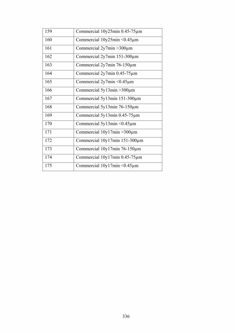
336
159 Commercial 10y25min 0.45-75µm
160 Commercial 10y25min <0.45µm
161 Commercial 2y7min >300µm
162 Commercial 2y7min 151-300µm
163 Commercial 2y7min 76-150µm
164 Commercial 2y7min 0.45-75µm
165 Commercial 2y7min <0.45µm
166 Commercial 5y13min >300µm
167 Commercial 5y13min 151-300µm
168 Commercial 5y13min 76-150µm
169 Commercial 5y13min 0.45-75µm
170 Commercial 5y13min <0.45µm
171 Commercial 10y17min >300µm
172 Commercial 10y17min 151-300µm
173 Commercial 10y17min 76-150µm
174 Commercial 10y17min 0.45-75µm
175 Commercial 10y17min <0.45µm
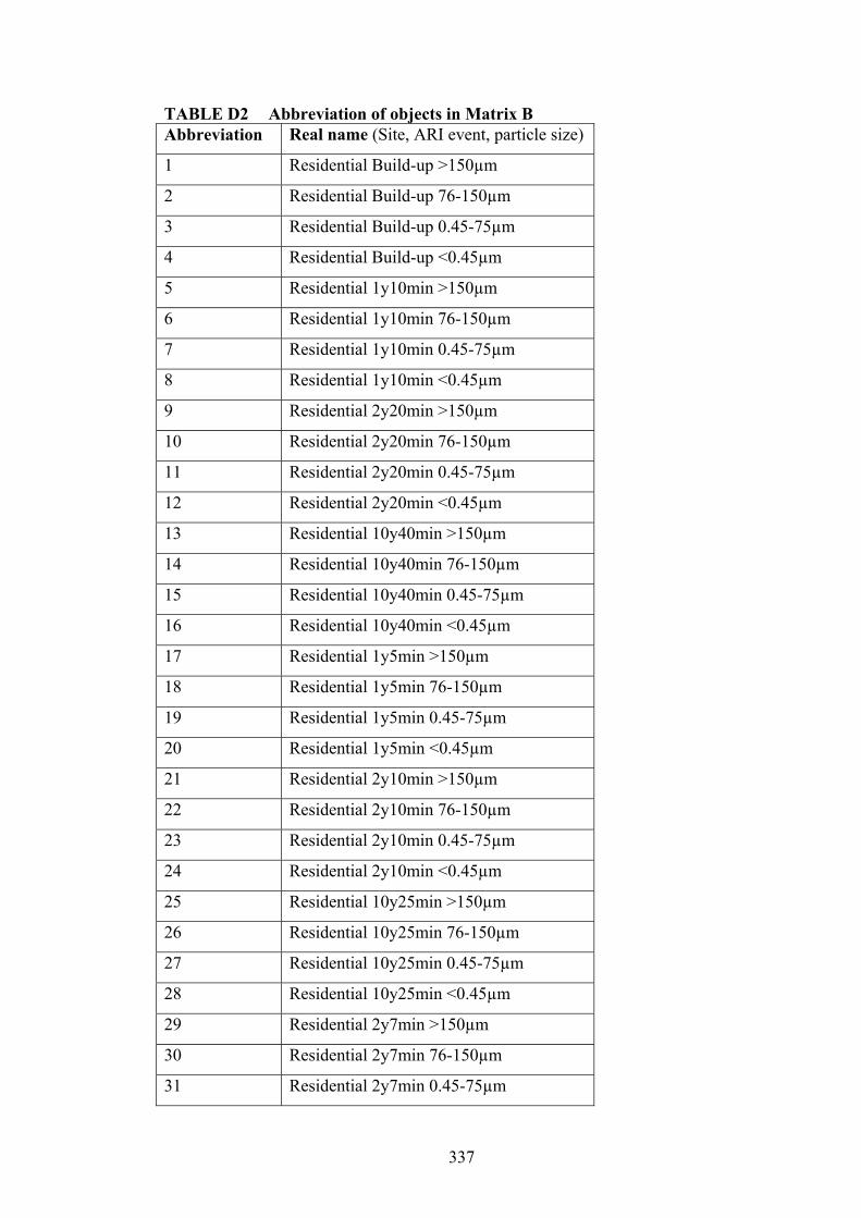
337
TABLE D2 Abbreviation of objects in Matrix B Abbreviation Real name (Site, ARI event, particle size)
1 Residential Build-up >150µm
2 Residential Build-up 76-150µm
3 Residential Build-up 0.45-75µm
4 Residential Build-up <0.45µm
5 Residential 1y10min >150µm
6 Residential 1y10min 76-150µm
7 Residential 1y10min 0.45-75µm
8 Residential 1y10min <0.45µm
9 Residential 2y20min >150µm
10 Residential 2y20min 76-150µm
11 Residential 2y20min 0.45-75µm
12 Residential 2y20min <0.45µm
13 Residential 10y40min >150µm
14 Residential 10y40min 76-150µm
15 Residential 10y40min 0.45-75µm
16 Residential 10y40min <0.45µm
17 Residential 1y5min >150µm
18 Residential 1y5min 76-150µm
19 Residential 1y5min 0.45-75µm
20 Residential 1y5min <0.45µm
21 Residential 2y10min >150µm
22 Residential 2y10min 76-150µm
23 Residential 2y10min 0.45-75µm
24 Residential 2y10min <0.45µm
25 Residential 10y25min >150µm
26 Residential 10y25min 76-150µm
27 Residential 10y25min 0.45-75µm
28 Residential 10y25min <0.45µm
29 Residential 2y7min >150µm
30 Residential 2y7min 76-150µm
31 Residential 2y7min 0.45-75µm
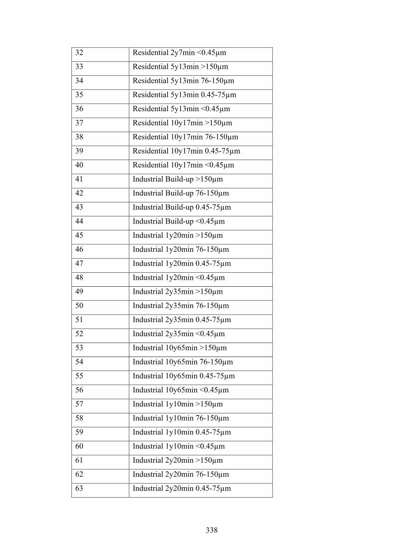
338
32 Residential 2y7min <0.45µm
33 Residential 5y13min >150µm
34 Residential 5y13min 76-150µm
35 Residential 5y13min 0.45-75µm
36 Residential 5y13min <0.45µm
37 Residential 10y17min >150µm
38 Residential 10y17min 76-150µm
39 Residential 10y17min 0.45-75µm
40 Residential 10y17min <0.45µm
41 Industrial Build-up >150µm
42 Industrial Build-up 76-150µm
43 Industrial Build-up 0.45-75µm
44 Industrial Build-up <0.45µm
45 Industrial 1y20min >150µm
46 Industrial 1y20min 76-150µm
47 Industrial 1y20min 0.45-75µm
48 Industrial 1y20min <0.45µm
49 Industrial 2y35min >150µm
50 Industrial 2y35min 76-150µm
51 Industrial 2y35min 0.45-75µm
52 Industrial 2y35min <0.45µm
53 Industrial 10y65min >150µm
54 Industrial 10y65min 76-150µm
55 Industrial 10y65min 0.45-75µm
56 Industrial 10y65min <0.45µm
57 Industrial 1y10min >150µm
58 Industrial 1y10min 76-150µm
59 Industrial 1y10min 0.45-75µm
60 Industrial 1y10min <0.45µm
61 Industrial 2y20min >150µm
62 Industrial 2y20min 76-150µm
63 Industrial 2y20min 0.45-75µm

339
64 Industrial 2y20min <0.45µm
65 Industrial 10y40min >150µm
66 Industrial 10y40min 76-150µm
67 Industrial 10y40min 0.45-75µm
68 Industrial 10y40min <0.45µm
69 Industrial 1y5min >150µm
70 Industrial 1y5min 76-150µm
71 Industrial 1y5min 0.45-75µm
72 Industrial 1y5min <0.45µm
73 Industrial 2y10min >150µm
74 Industrial 2y10min 76-150µm
75 Industrial 2y10min 0.45-75µm
76 Industrial 2y10min <0.45µm
77 Industrial 2y7min >150µm
78 Industrial 2y7min 76-150µm
79 Industrial 2y7min 0.45-75µm
80 Industrial 2y7min <0.45µm
81 Industrial 5y13min >150µm
82 Industrial 5y13min 76-150µm
83 Industrial 5y13min 0.45-75µm
84 Industrial 5y13min <0.45µm
85 Industrial 10y17min >150µm
86 Industrial 10y17min 76-150µm
87 Industrial 10y17min 0.45-75µm
88 Industrial 10y17min <0.45µm
89 Commercial Build-up >150µm
90 Commercial Build-up 76-150µm
91 Commercial Build-up 0.45-75µm
92 Commercial Build-up <0.45µm
93 Commercial 1y20min >150µm
94 Commercial 1y20min 76-150µm
95 Commercial 1y20min 0.45-75µm

340
96 Commercial 1y20min <0.45µm
97 Commercial 2y35min >150µm
98 Commercial 2y35min 76-150µm
99 Commercial 2y35min 0.45-75µm
100 Commercial 2y35min <0.45µm
101 Commercial 10y65min >150µm
102 Commercial 10y65min 76-150µm
103 Commercial 10y65min 0.45-75µm
104 Commercial 10y65min <0.45µm
105 Commercial 1y10min >150µm
106 Commercial 1y10min 76-150µm
107 Commercial 1y10min 0.45-75µm
108 Commercial 1y10min <0.45µm
109 Commercial 2y20min >150µm
110 Commercial 2y20min 76-150µm
111 Commercial 2y20min 0.45-75µm
112 Commercial 2y20min <0.45µm
113 Commercial 10y40min >150µm
114 Commercial 10y40min 76-150µm
115 Commercial 10y40min 0.45-75µm
116 Commercial 10y40min <0.45µm
117 Commercial 1y5min >150µm
118 Commercial 1y5min 76-150µm
119 Commercial 1y5min 0.45-75µm
120 Commercial 1y5min <0.45µm
121 Commercial 2y10min >150µm
122 Commercial 2y10min 76-150µm
123 Commercial 2y10min 0.45-75µm
124 Commercial 2y10min 0.45µm
125 Commercial 10y25min >150µm
126 Commercial 10y25min 76-150µm
127 Commercial 10y25min 0.45-75µm

341
128 Commercial 10y25min <0.45µm
129 Commercial 2y7min >150µm
130 Commercial 2y7min 76-150µm
131 Commercial 2y7min 0.45-75µm
132 Commercial 2y7min <0.45µm
133 Commercial 5y13min >150µm
134 Commercial 5y13min 76-150µm
135 Commercial 5y13min 0.45-75µm
136 Commercial 5y13min <0.45µm
137 Commercial 10y17min >150µm
138 Commercial 10y17min 76-150µm
139 Commercial 10y17min 0.45-75µm
140 Commercial 10y17min <0.45µm

342
TABLE D3 Loading coefficients of each variable in the predictions made
Predictors
Predicted pH EC TSS TDS DOC TOC IC Fe Mn
Al 0.1896 0.2260 0.0977 x x x x 0.2006 0.0269
Pb 0.5802 0.5216 0.3457 x x x x 1.1491 0.0247
Cu 0.2531 0.2740 x x x 0.3435 0.0809 x x
Cr 0.5147 0.4755 x x x 0.0153 0.0362 x x
Zn 0.9290 1.4437 x x 0.0081 x x x x
Cd 0.6454 0.5526 x x x 0.0775 0.7284 x x
PAH1 0.3582 0.5689 0.0391 x x 0.3251 0.2388 x x
PAH2 0.3175 0.6770 0.2117 x x 0.1610 0.2117 x x
PAH3 0.3175 0.6770 1.5231 x x 0.4958 0.4555 x x
x denotes not used in prediction; PAH1 = FLA and PYR; PAH2 = ACE and ACY; PAH3 = FLU, PHE, NAP, BaP, BaA and CHR

343
FIGURE D1 PCA scree plot of all the heavy metal data (175 objects) collected
from the three sites showing the elbow at the third principal component
-8 -6 -4 -2 0 2 4 6-3
-2
-1
0
1
2
3
001
002
003
004
005
006007
008
009010
011012013014
015016017
018019
020
021022023
024025
026027028
029030
031
032
033
034035
036037038
039040 041042043
044045
046047
048049
050
051
052053054
055
056057058
059060
061062
063
064
065066
067068
069070071072 073
074075 076
077078
079
080 081
082 083
084085
086087
088
089090
091092093
094
095
096097098
099100
101
102 103
104105 106
107108109110111112
113
114
115
116
117
118
119
120
121122123
124
125
126
127128129130
131
132
133134135
136137
138
139140
141
142143144
145
146147
148
149150
151152
153
154155 156157
158
159160
161162
163
164165
166167168
169170
171172173174
175
PC1 (41.1 %)
PC
2 (2
1.3
%)
FIGURE D2 Scores plot of PC1 vs PC3 from PCA on all heavy metal data
ELBOW
PC1 (41.1%)
PC3
(11.
2%)

344
-0.4 -0.3 -0.2 -0.1 0 0.1 0.2 0.3 0.4-0.8
-0.6
-0.4
-0.2
0
0.2
0.4
0.6
pH
EC
TOC
IC
DOCTSS
TDS
Fe
Zn Al Pb
Cu
Cd Cr
Mn
PC1 (41.1 %)
PC
2 (2
1.3
%)
FIGURE D3 Loadings plot (PC1 vs PC3) showing separation of metals on PC3
-0.4 -0.3 -0.2 -0.1 0 0.1 0.2 0.3 0.4-0.2
-0.1
0
0.1
0.2
0.3
0.4
0.5
0.6
pH EC
TOCIC
DOC
TSS
TDSFe
Zn
Al
Pb
Cu
Cd
Cr
Mn
PC1 (41.1 %)
PC
2 (2
1.3
%)
FIGURE D4 Loadings plot (PC1 vs PC2) showing separation of Zn from other
metals
PC1 (41.1%)
PC3
(11.
2%)

345
FIGURE D5 PCA scree plot of all the PAH data (140 objects) collected from
the three sites showing the elbow at the second principal component
FIGURE D6 PCA biplot of the PAH data collected from the three sites
ELBOW
Dissolved data
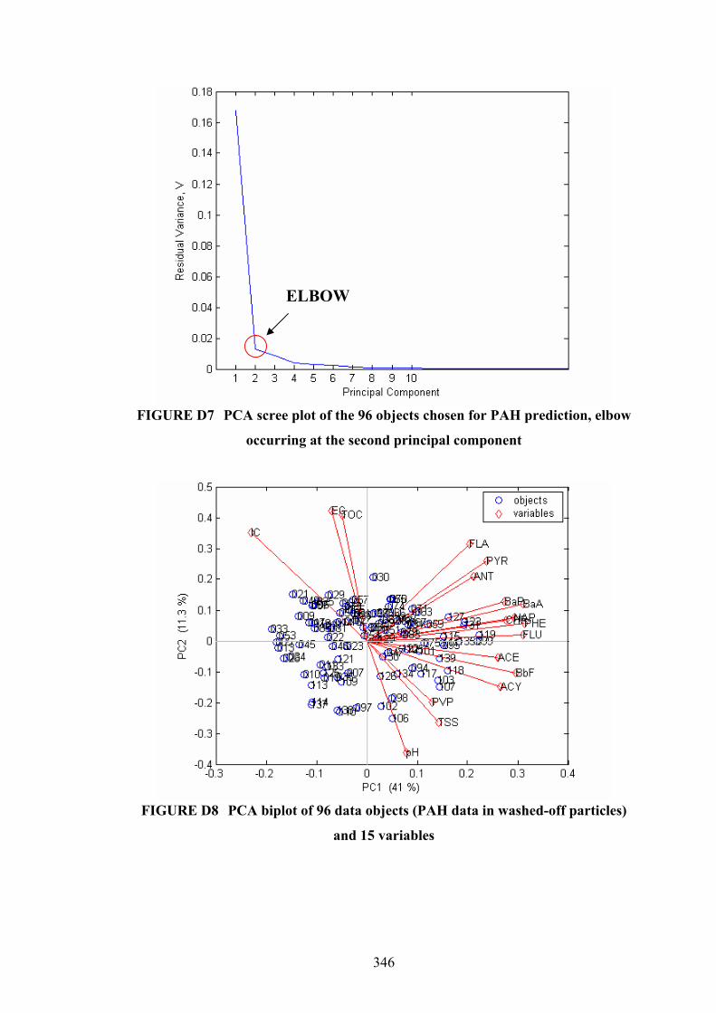
346
FIGURE D7 PCA scree plot of the 96 objects chosen for PAH prediction, elbow
occurring at the second principal component
FIGURE D8 PCA biplot of 96 data objects (PAH data in washed-off particles)
and 15 variables
ELBOW

347
FIGURE D9 Loadings plot (PC1 vs PC3) of the PAH data
FIGURE D10 Plot of observed versus predicted Cu concentrations using two
latent variables, with an SEP of 0.82
PC1 (41.1%)
PC3
(9.2
%)
Observed Cu concentrations log[mg/kg]
Pred
icte
d C
u co
ncen
tratio
ns lo
g[m
g/kg
]
------ Predicted -- Observed

348
FIGURE D11 Plot of observed versus predicted Cd concentrations using two
latent variables, with an SEP of 0.84
FIGURE D12 Plot of observed versus predicted Cr concentrations using two
latent variables, with an SEP of 0.94
Observed Cd concentrations log[mg/kg]
Pred
icte
d C
d co
ncen
tratio
ns lo
g[m
g/kg
]
------ Predicted -- Observed
Observed Cr concentrations log[mg/kg]
Pred
icte
d C
r con
cent
ratio
ns lo
g[m
g/kg
]
------ Predicted -- Observed
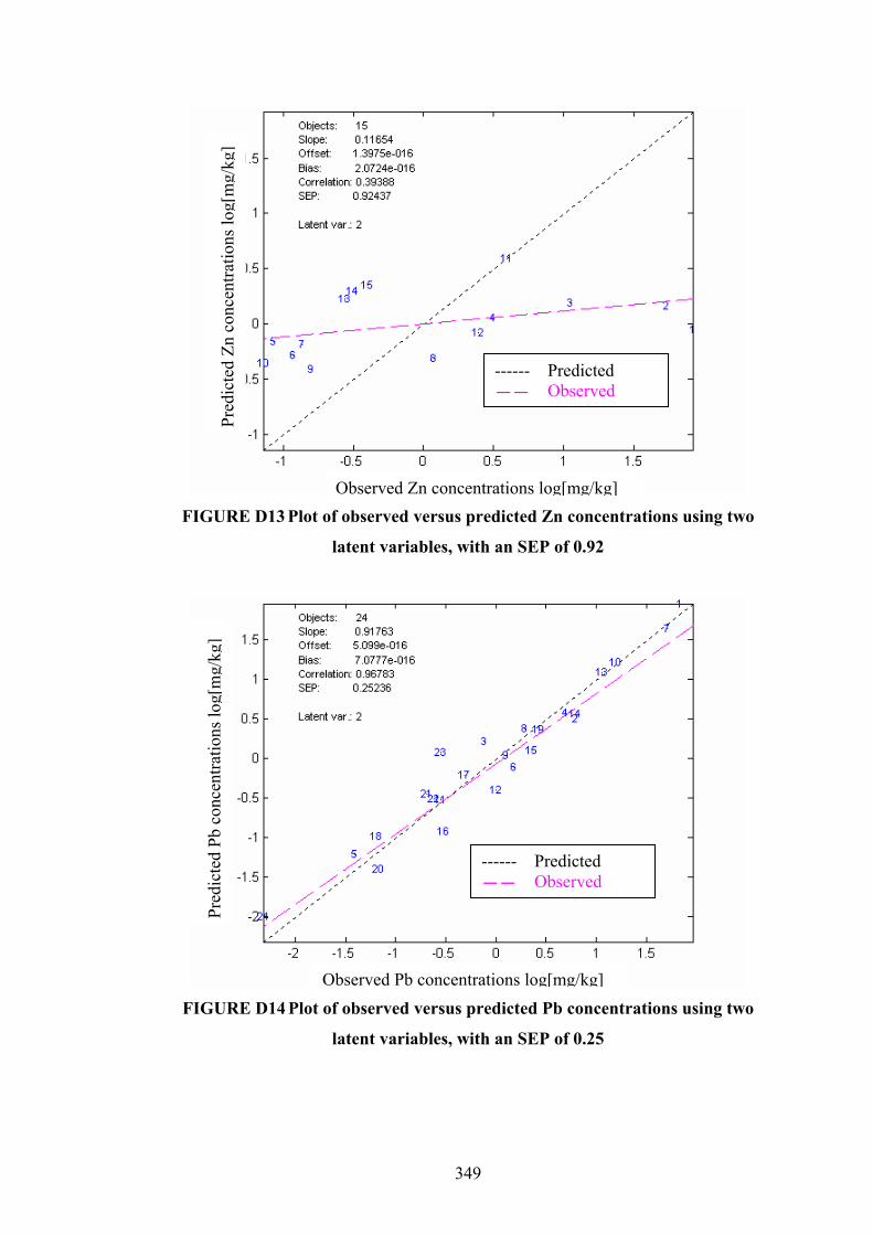
349
FIGURE D13 Plot of observed versus predicted Zn concentrations using two
latent variables, with an SEP of 0.92
FIGURE D14 Plot of observed versus predicted Pb concentrations using two
latent variables, with an SEP of 0.25
Observed Zn concentrations log[mg/kg]
Pred
icte
d Zn
con
cent
ratio
ns lo
g[m
g/kg
]
------ Predicted -- Observed
Observed Pb concentrations log[mg/kg]
Pred
icte
d Pb
con
cent
ratio
ns lo
g[m
g/kg
]
------ Predicted -- Observed

350
FIGURE D15 Plot of observed versus predicted concentrations of PAH group 1
using three latent variables, with an SEP of 0.84
FIGURE D16 Plot of observed versus predicted concentrations of PAH group 2
using four latent variables, with an SEP of 0.80
Observed concentrations log[mg/kg]
Pred
icte
d co
ncen
tratio
ns lo
g[m
g/kg
]
------ Predicted -- Observed
Observed concentrations log[mg/kg]
Pred
icte
d co
ncen
tratio
ns lo
g[m
g/kg
]
------ Predicted -- Observed

351
FIGURE D17 Plot of observed versus predicted concentrations of PAH group 3
using two latent variables, with an SEP of 0.86
Observed concentrations log[mg/kg]
Pred
icte
d co
ncen
tratio
ns lo
g[m
g/kg
]
------ Predicted -- Observed