large-scale visual recognition - inria
TRANSCRIPT
Large-scale visual recognition The bag-of-words representation Florent Perronnin, XRCE Hervé Jégou, INRIA
CVPR tutorial June 16, 2012

Outline Bag-of-words
Large or small vocabularies ?
Extensions for instance-level retrieval

Direct matching: the complexity issue
!! Assume an image described by m=1000 descriptors (dimension d=128) !! N*m=1 billion descriptors to index
!! Database representation in RAM: 128 GB with 1 byte per dimension
!! Search: m2* N * d elementary operations !! i.e., > 1014 " computationally not tractable !! The quadratic term m2: severely impacts the efficiency
Image search system
ranked image list
Image dataset: N > 1 million images
query
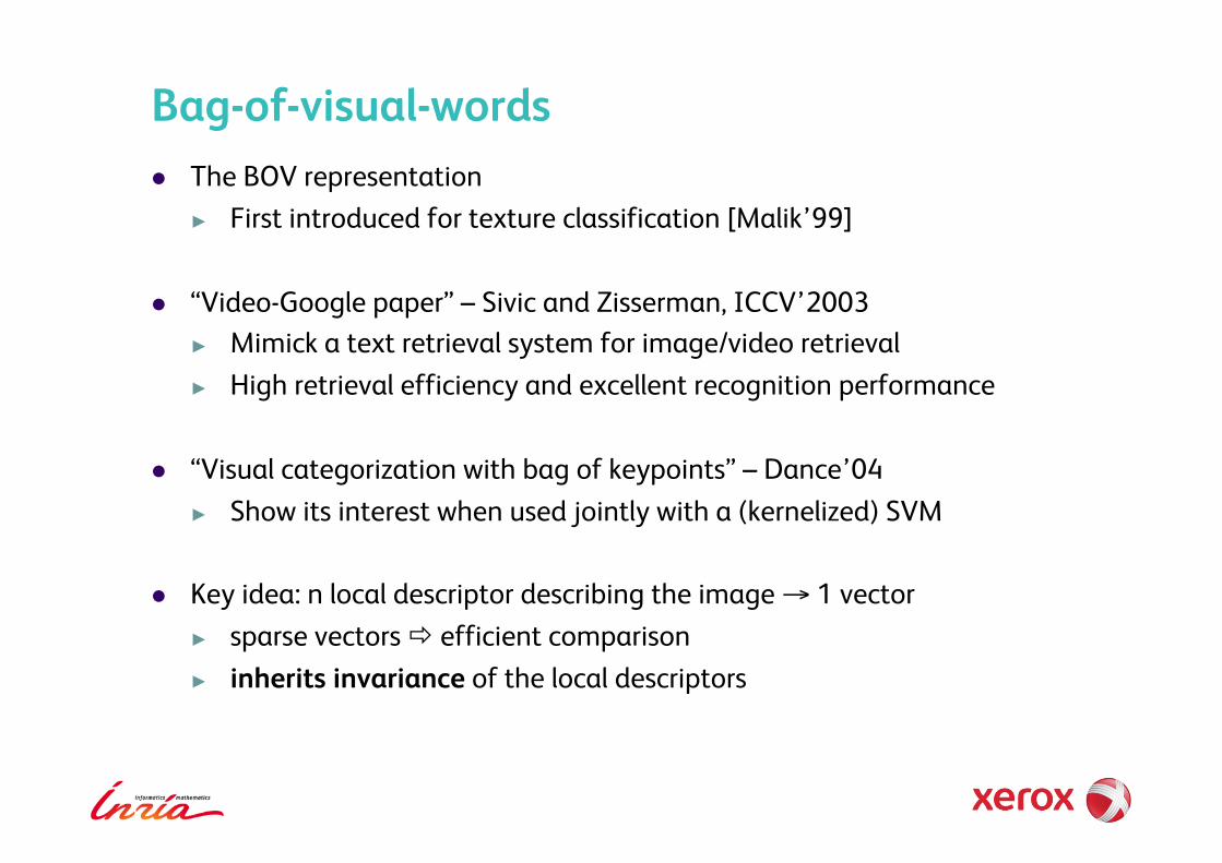
Bag-of-visual-words !! The BOV representation
!! First introduced for texture classification [Malik’99]
!! “Video-Google paper” – Sivic and Zisserman, ICCV’2003 !! Mimick a text retrieval system for image/video retrieval !! High retrieval efficiency and excellent recognition performance
!! “Visual categorization with bag of keypoints” – Dance’04 !! Show its interest when used jointly with a (kernelized) SVM
!! Key idea: n local descriptor describing the image ! 1 vector !! sparse vectors " efficient comparison !! inherits invariance of the local descriptors

Bag-of-visual words !! The goal: “put the images into words”, namely visual words
!! Input local descriptors are continuous !! Need to define what a “visual word is” !! Done by a quantizer q
q: d ! ! x ! c(x) ! !! q is typically a k-means
!! ! is called a “visual dictionary”, of size k !! A local descriptor is assigned to its nearest neighbor
q(x) = arg min ||x-w||2
w !
!! Quantization is lossy: we can not get back to the original descriptor !! But much more compact: typically 2-4 bytes/descriptor
x c(x)

Video Google – image search
!! Extract local descriptors !! Detector !! Describe the patch
!! Quantize all descriptors !! Subsequently compute the vector of frequencies !! Weight by IDF (rare if more important)
" TF-IDF vectors
!! Search similar vectors
!! Optionally: Re-ranking
Inverted file : sparse vectors
find most similar vectors results
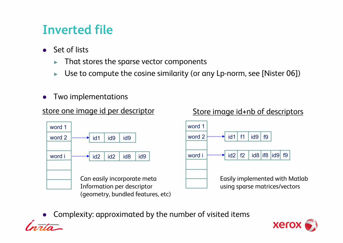
Inverted file !! Set of lists
!! That stores the sparse vector components !! Use to compute the cosine similarity (or any Lp-norm, see [Nister 06])
!! Two implementations
!! Complexity: approximated by the number of visited items
word 1
word 2
word i id2 id2 id8 id9
id1 id9 id9
word 1
word 2
word i id2 id8 id9
id1 id9
store one image id per descriptor Store image id+nb of descriptors
Easily implemented with Matlab using sparse matrices/vectors
f1 f9
f2 if8 f9
Can easily incorporate meta Information per descriptor (geometry, bundled features, etc)

Inverted file – Complexity !! Denote
!! pi = P(assign a descriptor to word i) !! N = number of image in database !! m = average # of descriptors / image
" The expected length of List i is given by: N*m*pi
!! The expected cost is :
!! Clusters of variable sizes negatively impacts this cost [Nister 06] !! Imbalance factor: !! measures the divergence from (optimal) uniform distribution (=1)
!! Strategies proposed to balance the clusters [Tavenard 11] ! but has an effect on search quality

Inverted file – Complexity !! Complexity is linear in the number of images
!! but small constant, in order of m/k E.g., C=0.01
!! Memory usage of an inverted file !! 1 million images " 8 GB (depending on m) !! Can be compressed [Jegou 09]

Inverted file – Boosting efficiency !! Stop-words
!! Method used in Text retrieval to discard uninformative words !! In image search: remove the s most frequent ones [Sivic 03] !! Impact on efficiency: assuming pi in decreasing order
replace by
!! But most frequent visual words are not that uninformative

Inverted file – Boosting efficiency !! Large vocabularies
!! Unlike in text, we decide the vocabulary size by choosing k ! for search quality and/or efficiency
!! Querying complexity: linear in 1/k !! Efficiency boosted by using a very large dictionary [Nister 06]
Outline Bag-of-words
Large or small vocabularies ?
Extensions for instance-level retrieval

Large vocabularies: assignment cost !! Large vocabularies are preferred [Nister 06]: high retrieval efficiency
!! But increased assignment cost, e.g., for k-means:
!! Structured quantizers: low quantization cost even for huge vocabularies !! Grid lattice quantizer [Tuytelaars 07] !! But poor performance in retrieval [Philbin 08] !! And very unbalanced [Pauleve 10]:

Large vocabularies with learned quantizer !! Hierarchical k-means [Nister 06]
!! K-means tree of height h
!! Branching factor b: !! Assignment Complexity:
!! Approximate k-means [Philbin 07] !! Based on approximate nearest neighbor search !! With parallel k-tree !! See later in this tutorial
HKM with b=3
Nister & Stewenius

Bag-of-words : another interpretation !! « Visual words » are a view of mind !! BOV " approximate k-NN search+voting
!! Implicitly define the neighborhood N(x) of a vector x as N(x) = { yi in Y : c(yi) = c(q) }
!! But, let assume: !! 2 descriptors in query !! 3 descriptors on database side
" 6 votes for 2x3 descriptors = contribution to the cosine similarity
!! Partial solution: pre-processing BOV with component-wise square rooting

Compromise on vocabulary size: k=20000
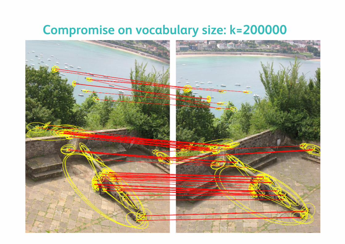
Compromise on vocabulary size: k=200000
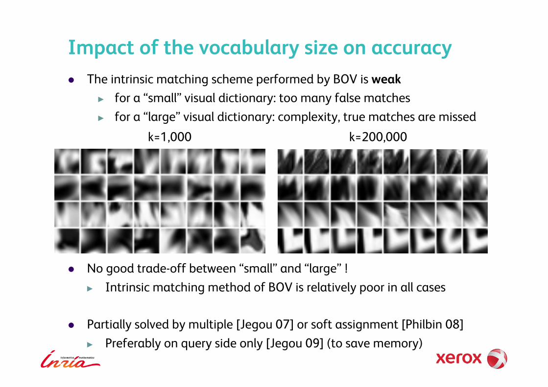
Impact of the vocabulary size on accuracy !! The intrinsic matching scheme performed by BOV is weak
!! for a “small” visual dictionary: too many false matches !! for a “large” visual dictionary: complexity, true matches are missed
k=1,000 k=200,000
!! No good trade-off between “small” and “large” ! !! Intrinsic matching method of BOV is relatively poor in all cases
!! Partially solved by multiple [Jegou 07] or soft assignment [Philbin 08] !! Preferably on query side only [Jegou 09] (to save memory)

Compromise on vocabulary size: k=20000

But with a better matching method (HE)…

Compromise on vocabulary size: k=200000
Interest of the voting interpretation !! Easy extended to incorporate
!! A better matching method [Jegou 08] !! Partial Geometrical information [Jegou 08, Zhao 10, …] !! Neighborhood information [Wu 09] !! … any method that requires to handle individual descriptors

Outline Bag-of-words
Large or small vocabularies ?
Extensions for instance-level retrieval

Geometrical verification !! Re-ranking based on full geometric verification [Philbin 07]
!! works very well but very costly !! Applied to a short-list only (typically, 100 images) !! for very large datasets, the number of distracting images is so high
that relevant images are not even short-listed!
0 0.1 0.2 0.3 0.4 0.5 0.6 0.7 0.8 0.9
1
1000 10000 100000 1000000 dataset size
rate
of r
elev
ant i
mag
es s
hort-
liste
d
20 images 100 images 1000 images
short-list size:

BOV 2
BOV 43064
Query
BOV 5890
BOV search in 1M images – ranks
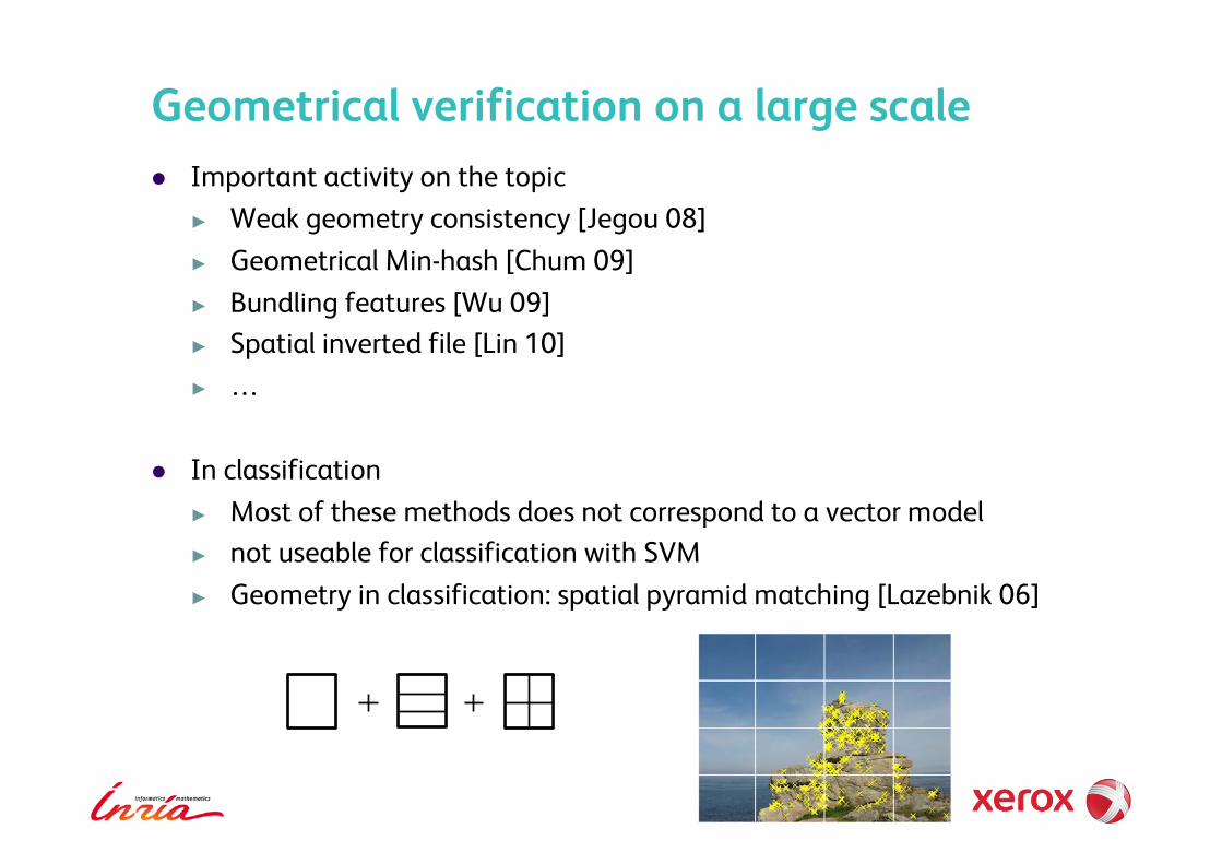
Geometrical verification on a large scale !! Important activity on the topic
!! Weak geometry consistency [Jegou 08] !! Geometrical Min-hash [Chum 09] !! Bundling features [Wu 09] !! Spatial inverted file [Lin 10] !! …
!! In classification !! Most of these methods does not correspond to a vector model !! not useable for classification with SVM !! Geometry in classification: spatial pyramid matching [Lazebnik 06]

Weak Geometry consistency !! WGC is a Hough transform
!! But do estimate a full geometrical transformation !! Separately estimate scalar quantities: rotation angle and log-scale !! Just it use to filter out the outliers
!! Implementation !! Store quantized dominant orientation and detector log-scale
! directly in the inverted file !! Two small hough histograms to collect the votes (16–32 bins/image)
!! Variation: Enhanced Weak Geometry consistency [Zhao 10] !! a.k.a visual phrases [Zhang 11] !! Deal with the translation only

Max = rotation angle between images
FILTERED!
Weak geometric consistency

PEAK
FILTERED!

BOV 2 HE+WGC 1
BOV 43064 HE+WGC 5
Query
BOV 5890 HE+WGC 4
Large scale impact: BOV search in 1M images

Query expansion in visual search
!! [Chum 07], “Total Recall”, ICCV 07
!! Different variants. Basic (shared) idea !! Process the list of results !! If some images are good (verified by spatial verification), use them !! To process some other augmented queries
12 results 41 resuls 44 results

Discriminative query expansion !! CVPR’12, [Arandjelovic 12] !! Learn a classifier on-the-fly
Artwork from Arandjelovic & Zisserman

Bag-of-words: concluding comments !! Practical solution: same ingredients as in text can be used
!! vector model ! useable with strong classifiers, in particular SVM !! query expansion [Chum’07] !! Or handle statistical phenomenons, e.g., Burstiness [Jegou’09]
!! With appropriate extension, state-of-the-art: !! Hamming Embedding !! Re-ranking with spatial verification !! Query-expansion
!! Limited to about a few million images on a server !! Caveat: memory usage !! See a demo at http://bigimbaz.inrialpes.fr

End

Algorithm 1: Transitive Query Expansion transitive queue = [query] results = {} While Queue not void query2 = queue.pop() results2 = search (query2) for all images in results2 image = results U {image} if high confidence in image (good spatial verification)
queue.push(image) return results
Total Recall: Automatic Query Expansion with a Generative Feature Model for Object Retrieval O. Chum, J. Philbin, J. Sivic, M. Isard, A. Zisserman, ICCV 07

Algorithm 2: Average Query Expansion descriptors = descriptors_interest_points (query) results = {} While descriptors “unstable” results2 = query (descriptors) for image in results2 results = results U {image} if image very reliable (spatial verification) dtran = transfo(descriptors_interest_points(image)) add dtran to descriptors
return results