large-scale sequential imperfect-information game solving

Large-Scale SequentialImperfect-Information Game Solving:Theoretical Foundations and Practical

Algorithms with GuaranteesChristian Kroer

Thursday 12th January, 2017

School of Computer ScienceCarnegie Mellon University

Pittsburgh, PA 15213

Thesis Committee:Tuomas Sandholm, Chair

Geoffrey J. GordonFatma Kılınc-Karzan

Vince Conitzer, Duke UniversityYurii Nesterov, Universite catholique de Louvain

Submitted in partial fulfillment of the requirementsfor the degree of Doctor of Philosophy.

Copyright c© 2016 Christian Kroer

Keywords: equilibrium finding, extensive-form games, sequential games, imperfect-information games,Nash equilibrium, abstraction, convex optimization, first-order methods, limited lookahead

AbstractGame-theoretic equilibrium concepts provide a sound definition of how rational agents

should act in multiagent settings. To operationalize them, they have to be accompanied bytechniques to compute equilibria. We study the computation of equilibria for extensive-formgames, a broad game class that can model sequential interaction, imperfect information, andoutcome uncertainty. Practical equilibrium computation in extensive-form games relies on twocomplementary methods: abstraction methods and sparse iterative equilibrium-finding algo-rithms. These methods are necessary in order to handle the size of many real-world games.

We present new algorithmic and structural results for both parts of extensive-form gamesolving. We introduce state-of-the-art theoretical guarantees on the performance of our algo-rithms, and first-of-their-kind guarantees on the solution quality of abstractions for large games.

For abstraction, we develop new theoretical guarantees on the solution quality of equilibriacomputed in abstractions. We develop new results for several types of games and abstractions:discrete and continuous extensive-form games, and perfect and imperfect-recall abstractions.For all settings, our results are the first algorithm-agnostic solution-quality guarantees. Ad-ditionally, even compared to algorithm-specific results, our approach leads to exponentiallystronger bounds than prior results, and extend to more general games and abstractions.

For equilibrium computation, we focus on the formulation of an extensive-form two-playerzero-sum Nash equilibrium as a bilinear saddle-point problem. This allows us to leverage meth-ods from the convex optimization literature. We consider a smoothing method based on a dilatedentropy function. We prove bounds on the strong convexity and polytope diameter associatedwith this function that are significantly stronger than bounds for prior smoothing methods. Thisleads to the state-of-the-art in convergence rate for sparse iterative methods for computing aNash equilibrium. Our results can also be viewed more generally as strong convexity results fora class of convex polytopes called treeplexes. These results could be of independent interest inother sequential decision-making settings.

Finally, we develop new solution concepts and associated algorithmic results for gameswhere opponents have limited lookahead.

Contents

1 Introduction 11.1 Algorithms for computing equilibria (Chapter 3) . . . . . . . . . . . . . . . . . . . . . . . . 2

1.1.1 Completed work . . . . . . . . . . . . . . . . . . . . . . . . . . . . . . . . . . . . 21.1.2 Proposed work (Section 3.3) . . . . . . . . . . . . . . . . . . . . . . . . . . . . . . 3

1.2 Abstraction for large games (Chapter 4) . . . . . . . . . . . . . . . . . . . . . . . . . . . . 31.2.1 Completed work . . . . . . . . . . . . . . . . . . . . . . . . . . . . . . . . . . . . 31.2.2 Proposed work (Section 4.4) . . . . . . . . . . . . . . . . . . . . . . . . . . . . . . 5

1.3 Limited lookead (Chapter 5) . . . . . . . . . . . . . . . . . . . . . . . . . . . . . . . . . . 51.3.1 Completed work . . . . . . . . . . . . . . . . . . . . . . . . . . . . . . . . . . . . 51.3.2 Proposed work (Section 5.7) . . . . . . . . . . . . . . . . . . . . . . . . . . . . . . 6

1.4 Structure of this document . . . . . . . . . . . . . . . . . . . . . . . . . . . . . . . . . . . 6

2 Notation 72.1 Extensive-form games . . . . . . . . . . . . . . . . . . . . . . . . . . . . . . . . . . . . . 72.2 Value functions for an extensive-form game . . . . . . . . . . . . . . . . . . . . . . . . . . 82.3 Equilibrium concepts . . . . . . . . . . . . . . . . . . . . . . . . . . . . . . . . . . . . . . 9

3 Algorithms for computing equilibria 103.1 Related work . . . . . . . . . . . . . . . . . . . . . . . . . . . . . . . . . . . . . . . . . . 103.2 Accelerating first-order methods through better smoothing . . . . . . . . . . . . . . . . . . 11

3.2.1 Introduction . . . . . . . . . . . . . . . . . . . . . . . . . . . . . . . . . . . . . . . 113.2.2 Problem setup . . . . . . . . . . . . . . . . . . . . . . . . . . . . . . . . . . . . . 123.2.3 Optimization setup . . . . . . . . . . . . . . . . . . . . . . . . . . . . . . . . . . . 133.2.4 Treeplexes . . . . . . . . . . . . . . . . . . . . . . . . . . . . . . . . . . . . . . . 153.2.5 Distance-generating functions with bounded strong convexity . . . . . . . . . . . . 173.2.6 Instantiating FOMs for extensive-form game solving . . . . . . . . . . . . . . . . . 193.2.7 Sampling . . . . . . . . . . . . . . . . . . . . . . . . . . . . . . . . . . . . . . . . 193.2.8 Discussion of theoretical improvements . . . . . . . . . . . . . . . . . . . . . . . . 213.2.9 Numerical experiments . . . . . . . . . . . . . . . . . . . . . . . . . . . . . . . . . 233.2.10 Conclusions . . . . . . . . . . . . . . . . . . . . . . . . . . . . . . . . . . . . . . . 25

3.3 Proposed work . . . . . . . . . . . . . . . . . . . . . . . . . . . . . . . . . . . . . . . . . 26

4 Abstraction for large games 284.1 Perfect-recall abstraction . . . . . . . . . . . . . . . . . . . . . . . . . . . . . . . . . . . . 29

4.1.1 Introduction . . . . . . . . . . . . . . . . . . . . . . . . . . . . . . . . . . . . . . . 29

iv

4.1.2 Framework . . . . . . . . . . . . . . . . . . . . . . . . . . . . . . . . . . . . . . . 294.1.3 Reward-approximation and information-approximation error terms . . . . . . . . . . 324.1.4 Lifted strategies from abstract equilibria have bounded regret . . . . . . . . . . . . . 334.1.5 Abstraction algorithms and complexity . . . . . . . . . . . . . . . . . . . . . . . . 354.1.6 Experiment . . . . . . . . . . . . . . . . . . . . . . . . . . . . . . . . . . . . . . . 414.1.7 Discussion . . . . . . . . . . . . . . . . . . . . . . . . . . . . . . . . . . . . . . . 42

4.2 Imperfect-recall abstraction . . . . . . . . . . . . . . . . . . . . . . . . . . . . . . . . . . . 434.2.1 Introduction . . . . . . . . . . . . . . . . . . . . . . . . . . . . . . . . . . . . . . . 434.2.2 Perfect-recall refinements and abstraction concepts . . . . . . . . . . . . . . . . . . 444.2.3 Strategies from abstract near-equilibria have bounded regret . . . . . . . . . . . . . 464.2.4 Complexity and algorithms . . . . . . . . . . . . . . . . . . . . . . . . . . . . . . . 484.2.5 Experiments . . . . . . . . . . . . . . . . . . . . . . . . . . . . . . . . . . . . . . 504.2.6 Discussion . . . . . . . . . . . . . . . . . . . . . . . . . . . . . . . . . . . . . . . 52

4.3 Discretizing continuous action spaces . . . . . . . . . . . . . . . . . . . . . . . . . . . . . 524.3.1 Introduction . . . . . . . . . . . . . . . . . . . . . . . . . . . . . . . . . . . . . . . 524.3.2 Continuous action spaces . . . . . . . . . . . . . . . . . . . . . . . . . . . . . . . . 534.3.3 Discretization model . . . . . . . . . . . . . . . . . . . . . . . . . . . . . . . . . . 544.3.4 Overview of our approach . . . . . . . . . . . . . . . . . . . . . . . . . . . . . . . 564.3.5 Discretization quality bounds . . . . . . . . . . . . . . . . . . . . . . . . . . . . . 574.3.6 Discretization algorithms . . . . . . . . . . . . . . . . . . . . . . . . . . . . . . . . 574.3.7 Applications . . . . . . . . . . . . . . . . . . . . . . . . . . . . . . . . . . . . . . 614.3.8 Differences to abstraction practice in poker . . . . . . . . . . . . . . . . . . . . . . 624.3.9 Conclusions . . . . . . . . . . . . . . . . . . . . . . . . . . . . . . . . . . . . . . . 62

4.4 Proposed work . . . . . . . . . . . . . . . . . . . . . . . . . . . . . . . . . . . . . . . . . 63

5 Limited lookahead in sequential games 655.1 Introduction . . . . . . . . . . . . . . . . . . . . . . . . . . . . . . . . . . . . . . . . . . . 655.2 Model of limited lookahead . . . . . . . . . . . . . . . . . . . . . . . . . . . . . . . . . . . 665.3 Complexity . . . . . . . . . . . . . . . . . . . . . . . . . . . . . . . . . . . . . . . . . . . 66

5.3.1 Nash equilibrium . . . . . . . . . . . . . . . . . . . . . . . . . . . . . . . . . . . . 665.3.2 Commitment strategies . . . . . . . . . . . . . . . . . . . . . . . . . . . . . . . . . 67

5.4 Algorithms . . . . . . . . . . . . . . . . . . . . . . . . . . . . . . . . . . . . . . . . . . . 685.5 Experiments . . . . . . . . . . . . . . . . . . . . . . . . . . . . . . . . . . . . . . . . . . . 705.6 Conclusions and future work . . . . . . . . . . . . . . . . . . . . . . . . . . . . . . . . . . 745.7 Proposed work . . . . . . . . . . . . . . . . . . . . . . . . . . . . . . . . . . . . . . . . . 75

6 Timeline 76

7 A brief overview of my non-thesis research 77

Bibliography 78

Chapter 1

Introduction

Game-theoretic solution concepts provide a sound notion of rational behavior in multiagent settings. Tooperationalize equilibria, they have to be accompanied by computational techniques for identifying them.Thus, equilibrium computation has emerged as a central topic in economics and computation [Gilpin andSandholm, 2007b, Jiang and Leyton-Brown, 2011, Lipton et al., 2003, Littman and Stone, 2003, Zinkevichet al., 2007, Koller et al., 1996, Daskalakis et al., 2015, von Stengel, 1996]. In this thesis we focus mainlyon extensive-form games. Extensive-form games are a broad class of games that can model sequential andsimultaneous moves, outcome uncertainty, and imperfect information. This includes real-world settingssuch as negotiation, sequential auctions, security games, cybersecurity games, recreational games such aspoker and billiards, and certain medical treatment settings [Archibald and Shoham, 2009, Lisy et al., 2016,Munoz de Cote et al., 2013, Sandholm, 2010, DeBruhl et al., 2014, Chen and Bowling, 2012].

The primary benchmark for large-scale equilibrium-finding is the annual computer poker competition(ACPC). Each year, research labs and individual hobbyists submit poker bots which are faced off in com-petition. For many years, all of the most successful bots have been based on equilibrium-finding tech-niques [ACPC, 2016, Sandholm, 2010, Brown et al., 2015]. More specifically, these bots employ the fol-lowing technique: First, the game is abstracted to generate a smaller game. Then the abstract game is solvedfor (near-)equilibrium. Then, the strategy from the abstract game is mapped back to the original game. Thisprocess is shown pictorally in Figure 1.1. The figure suggests that an ε-Nash equilibrium is obtained in thefull game. Current practical methods have no such guarantee on the quality of the equilibrium in the fullgame. Furthermore, practical abstractions are so large that exact Nash equilibria can’t be computed, even inthe abstraction. Instead, sparse iterative methods are applied, which converge to a Nash equilibrium in thelimit.

This thesis proposal explores and develops theoretical foundations for all steps of the solution processdescribed above. Secion 3 develops state-of-the-art convergence rate bounds for sparse iterative solvers.Section 4 ameliorates the lack of guarantees on abstraction solution quality by developing some of the first,and by far the strongest, bounds on solution quality. Section 5 develops new solution concepts for settingswhere a rational player is facing one or more myopic adversaries. In such a setting rationality may be anoverly pessimistic assumption, and instead we present a model of limited lookahead in EFGs.

The next three sections will give a brief overview of the results obtained so far on each of the equilibrium-finding dimensions, as well as briefly mention the proposed extensions.

1

Nash equilibriumε-Nash equilibrium

Abstracted game

(automated) Abstraction

Equilibrium-finding algorithm

Map to real game

Real game

Figure 1.1: An overview of the general abstraction approach (figure borrowed from Ganzfried and Sand-holm [2012]).

1.1 Algorithms for computing equilibria (Chapter 3)

This chapter focuses on sparse iterative methods for large-scale equilibrium computation. In particular, weinvestigate the application of first-order methods (FOMs) to the computation of equilibria in two-playerzero-sum games. The application of FOMs relies on three core ingredients: (1) the sequence-form trans-formation [von Stengel, 1996] for obtaining a bilinear saddle-point formulation, (2) convex minimizationalgorithms such as the excessive gap technique (EGT) [Nesterov, 2005a] or mirror prox [Nemirovski, 2004],and (3) smoothing techniques for the strategy spaces of the two players. The third part is currently not wellunderstood.

1.1.1 Completed work

Hoda et al. [2010] introduced a class of smoothing techniques that can be applied to EFGs. However, theconvergence rate bounds obtained from the results of Hoda et al. [2010] have a significantly worse depen-dence on the EFG size than CFR. We show that a much better dependence on game parameters can beachieved by focusing on the entropy function as a smoothing technique for each information set. This isdone by carefully choosing information-set weights such that a desirable smoothing function for the gametree is obtained by summing over the weighted entropy functions for each information sets. Our resultleads to the strongest known convergence rate for sparse iterative methods, achieving a dependence on gameconstants that is much stronger than that of Hoda et al. [2010], while maintaining a 1/T convergence rate.In particular, our strong convexity result is the first to achieve no dependence on the branching branchingfactor associated with a player. Furthermore, we introduce a new class of gradient estimators that allowinstantiation of stochastic FOMs such as stochastic mirror prox [Juditsky et al., 2011]. Finally, we showexperimentally that EGT and mirror prox instantiated with our smoothing technique leads to better practicalconvergence rates than CFR for medium-to-high accuracy solutions on medium-sized games.

Part of this work was published at EC-2015 [Kroer et al., 2015]. A follow-up manuscript is available at(currently unpublished, cite arXiv .

1.1.2 Proposed work (Section 3.3)

While our current results are state-of-the-art for theoretical convergence rates for sparse iterative methods,they are not the practical state-of-the-art. In practice, CFR algorithms are still preferred. We propose ex-tending our theoretical work by experimentally findings ways to scale up FOMs to be competitive with CFRalgorithms. Our two most promising ideas for achieving this are 1) heuristic aggressive stepsizing for EGTcoupled with checks of the excessive gap condition, and 2) better initialization of EGT (preliminary exper-imental results suggest that even simple tweaks to the starting point can have several orders of magnitudeimpact on convergence rate). The success of this approach will be measured by showing that FOMs canoutperform the leading CFR-like algorithm on real-world games. Specifically, we will consider one or bothof the following games:• Large texas holdem poker endgames. An endgame is, at a high level, an extensive-form game con-

structed ad-hoc to represent some subset of the game. Endgames are currently solved with CFR+, andrepresent the smallest class of games where FOMs can have practical impact.

• No limit Texas hold’em (NLTHE) game abstractions. NLTHE is the current frontier of large-scaleEFG solving, where many state-of-the-art contemporary bots are more exploitable than always folding(i.e. laying down your hand immediately) [Lisy and Bowling, 2017].

Theoretically, we propose extending our results by developing corresponding lower bounds on the con-vergence rates achievable with the class of entropy-based smoothing functions we consider. Furthermore, wepropose showing upper and/or lower bounds on the convergence rate achievable with l2 smoothing. Ideally,this will allow us to show that entropy-based smoothing is theoretically superior to l2 smoothing for EFGs.This would complement experimental results from Hoda et al. [2010], which found entropy smoothing tobe superior.

Finally, we propose the development of sparse iterative methods for computing Nash-equilibrium refine-ments. Polynomial-time algorithms are known for refinements such as normal-form proper and quasi-perfectequilibria [Miltersen and Sørensen, 2008, 2010]. However, these algorithms rely on solving one or morelinear programs, usually relying on modifications to the sequence-form LP of von Stengel [1996]. As withNash equilibria, such LP formulations are unlikely to be practical for large-scale games. Instead, we proposeleveraging a perturbed sequence-form polytope in the standard bilinear saddle-point formulation, and thenfocus on solving this saddle-point problem directly. For small-enough perturbations, this should lead to anapproximate Nash equilibrium refinement.

1.2 Abstraction for large games (Chapter 4)

As mentioned previously, practical equilibrium computation usually relies on dimensionality reductionthrough creating an abstracted game first. This chapter focuses on abstraction methods for reducing thedimensionality of extremely large games. Practical abstraction algorithms for EFGs have all been withoutany solution quality bounds [Gilpin and Sandholm, 2006, 2007a, Gilpin et al., 2007, Gilpin and Sandholm,2008, Ganzfried and Sandholm, 2014]. This chapter ameliorates this fact by developing some of the firsttheoretical results on the quality of equilibria computed in abstractions of EFGs.


We have developed theoretical guarantees on solution quality of equilibria in several settings.

Perfect-recall abstraction. We develop the first algorithm-agnostic bounds on solution quality for equi-libria computed in perfect-recall abstractions. This work also improves the best prior bounds, whichwere specific to CFR, by an exponential amount. In particular, the payoff error in prior bounds had alinear dependence on the number of information sets, whereas the payoff error in our bounds has nodependence on the number of information sets. Our result is obtained by introducing a new methodfor mapping abstract strategies to the full game, and leverages a new equilibrium refinement in theanalysis. Using this framework, we develop the first general lossy extensive-form game abstractionmethod with bounds. Experiments show that it finds a lossless abstraction when one is available andlossy abstractions when smaller abstractions are desired.

We also develop the first complexity results on computing good abstractions of EFGs. Prior abstrac-tion algorithms typically operate level by level in the game tree. We introduce the extensive-formgame tree isomorphism and action subset selection problems, both important subproblems for com-puting abstractions on a level-by-level basis. We show that the former is graph isomorphism complete,and the latter NP-complete. This suggests that level-by-level abstraction is, in general, a computation-ally difficult problem. We also prove that level-by-level abstraction can be too myopic and thus fail tofind even obvious lossless abstractions.

This work was published at EC-2014 [Kroer and Sandholm, 2014]

Imperfect-recall abstraction. Imperfect-recall abstraction has emerged as the leading paradigm for prac-tical large-scale equilibrium computation in imperfect-information games. However, imperfect-recallabstractions are poorly understood, and only weak algorithm-specific guarantees on solution qualityare known. We develop the first general, algorithm-agnostic, solution quality guarantees for Nashequilibria and approximate self-trembling equilibria (a new solution concept that we introduce) com-puted in imperfect-recall abstractions, when implemented in the original (perfect-recall) game. Ourresults are for a class of games that generalizes the only previously known class of imperfect-recallabstractions for which any such results have been obtained. Further, our analysis is tighter in twoways, each of which can lead to an exponential reduction in the solution quality error bound.

We then show that for extensive-form games that satisfy certain properties, the problem of computinga bound-minimizing abstraction for a single level of the game reduces to a clustering problem, wherethe increase in our bound is the distance function. This reduction leads to the first imperfect-recallabstraction algorithm with solution quality bounds. We proceed to show a divide in the class of ab-straction problems. If payoffs are at the same scale at all information sets considered for abstraction,the input forms a metric space, and this immediately yields a 2-approximation algorithm for abstrac-tion. Conversely, if this condition is not satisfied, we show that the input does not form a metric space.Finally, we provide computational experiments to evaluate the practical usefulness of the abstractiontechniques. They show that running counterfactual regret minimization on such abstractions leads togood strategies in the original games.

This work was published at EC-2016 [Kroer and Sandholm, 2016a]

Discretization of continuous games. While EFGs are a very general class of games, most solution algo-rithms require discrete, finite games. In contrast, many real-world domains require modeling withcontinuous action spaces. This is usually handled by heuristically discretizing the continuous actionspace without solution quality bounds. Leveraging our results on abstraction solution quality, we de-velop the first framework for providing bounds on solution quality for discretization of continuousaction spaces in extensive-form games. For games where the error is Lipschitz-continuous in the dis-tance of a continuous point to its nearest discrete point, we show that a uniform discretization of the

space is optimal. When the error is monotonically increasing in distance to nearest discrete point,we develop an integer program for finding the optimal discretization when the error is described bypiecewise linear functions. This result can further be used to approximate optimal solutions to generalmonotonic error functions.

This work was published at AAMAS-2015 [Kroer and Sandholm, 2015b]


While the above lines of work have provided much-needed theoretical foundations for the area of abstractionin EFGs, there is still a lot of work to do in order to bridge the gap to practical abstraction work. Allabstraction algorithms mentioned in the preceding section require either 1) solving an integer program whosesize is on the order of magnitude of the game tree (this can be improved to just the signal tree for games ofordered signals) [Kroer and Sandholm, 2014], or 2) solving for abstractions level-by-level with prohibitivelystrong constraints on the type of abstraction allowed [Kroer and Sandholm, 2016a].

We propose developing practical methods for computing abstractions, while retaining bounds on thesolution quality. One way to do this is by extending our framework for bounding abstraction quality to allowadditional worst-case assumptions about paths in the game tree that our current framework cannot providebounds for. This will greatly expand the set of feasible abstractions, thereby making the computationalproblem easier. Hopefully, it will also allow analysis of a general level-by-level abstraction algorithm.An alternative approach would be to make additional assumptions about the game structure, potentiallyassuming structure that is similar to that of games of ordered signals [Gilpin and Sandholm, 2007b].

We will attempt one or more of the following goals:• Compute the first strategy with a meaningful bound on regret in NLTHE (through solving an abstract

game).• Show that existing practical abstraction algorithms have bounded solution quality.• Show an impossibility result stating that the kind of abstraction employed in practice cannot lead to

meaningful ex-ante bounds on solution quality.

1.3 Limited lookead (Chapter 5)

In some application domains, the assumption of perfect rationality might not be practical, or even useful,as opponents might display exploitable behavior that the perfect rationality assumption does not allow ex-ploitation of. In order to model such settings, we initiate the game-theoretic study of limited lookahead inimperfect-information games.

This model has applications such as biological games, where the goal is to steer an evolutionary oradaptation process (which typically acts myopically with lookahead 1) [Sandholm, 2015], and securitygames where opponents are often assumed to be myopic (as makes sense when the number of adversariesis large [Yin et al., 2012]). Furthermore, investigating how well a rational player can exploit a limited-lookahead player lends insight into the limitations and risks of using limited-lookahead algorithms in mul-tiagent decision making.


We generalize limited-lookahead research to imperfect-information games and a game-theoretic approach.We study the question of how one should act when facing an opponent whose lookahead is limited along

multiple axes: lookahead depth, whether the opponent(s), too, have imperfect information, and how theybreak ties. We characterize the hardness of finding a Nash equilibrium or an optimal commitment strategy foreither player, showing that in some of these variations the problem can be solved in polynomial time whilein others it is PPAD-hard or NP-hard. We proceed to design algorithms for computing optimal commitmentstrategies for when the opponent breaks ties 1) favorably, 2) according to a fixed rule, or 3) adversarially. Theimpact of limited lookahead is then investigated experimentally. The limited-lookahead player often obtainsthe value of the game if she knows the expected values of nodes in the game tree for some equilibrium,but we prove this is not sufficient in general. Finally, we study the impact of noise in those estimates anddifferent lookahead depths. This uncovers a lookahead pathology.

This work was published at IJCAI-2015 [Kroer and Sandholm, 2015c]


While our current model of limited lookahead can model certain myopic adversaries, it has one impor-tant weakness: it does not allow for modeling of uncertainty over the exact myopic behavior of the oppo-nents. We propose extending our current model of limited lookahead to include a distribution over limited-lookahead opponent models. This will allow much more general modeling of myopic behavior, as wellas allow for computing robust strategies for exploiting a myopic opponent. Depending on the specific as-sumptions made, this can make the computation of the associated solution concepts significantly harder. Wepropose managing this increased complexity by viewing the problem through a robust optimization lends.

1.4 Structure of this document

This chapter gave a high-level description of each of the dimensions of sequential game solving consideredin this thesis. The following chapters will go into more depth on our results and proposed research directionsfor each topic. Chapter 2 develops some notation necesary in order to read the technical sections of thefollowing chapters. Chapter 2 should not be neccesary in order to understand the introductory and proposedwork sections of each chapter. Chapters 3, 4 and 5 present my current and proposed work on first-ordermethods to compute equilibria, abstraction methods, and new models of limited-lookahead adversaries.These chapters include fairly detailed technical sections, but the gist of the chapters can be gleaned from theintroductory sections as well as proposed work sections.

Finally, Chapter 7 will briefly discuss some other research work that I’ve done during my doctoralstudies.

Chapter 2

Notation

This section introduces some general notation for EFGs that we will use throughout most of this proposal.Chapter 3 is largely independent of this notation, and so can safely be read in isolation. Chapters 4 and 5rely more heavily on the notation described here for formally describing the obtained results.

2.1 Extensive-form games

An extensive-form game (EFG) Γ is a tuple 〈N,A, S, Z,H, σ0, u, I〉. N is the set of players. A is the setof all actions. S is a set of nodes corresponding to sequences of actions. They describe a tree with rootnode r ∈ S. At each node s, some Player i is active with actions As, and each branch at s denotes adifferent choice in As. Let tsa be the node transitioned to by performing action a ∈ As at node s. The setof all nodes where Player i is active is called Si. The set of leaf nodes is denoted by Z ⊂ S. For eachleaf node z, Player i receives a reward of ui(z). We assume, WLOG., that all utilities are non-negative.Zs is the subset of leaf nodes reachable from a node s. Hi ⊆ H is the set of heights in the game treewhere Player i acts. H0 is the set of heights where nature acts. σ0 specifies the probability distribution fornature, with σ0(s, a) denoting the probability of nature choosing outcome a at node s. Ii ⊆ I is the set ofinformation sets where Player i acts. Ii partitions Si. For any two nodes s1, s2 ∈ I ∈ Ii, Player i cannotdistinguish among them, and As1 = As2 . We let X(s) denote the set of information set and action pairs I, ain the sequence leading to a node s, including nature. We let X−i(s), Xi(s) ⊆ X(s) be the subset of thissequence such that actions by the subscripted player(s) are excluded or exclusively chosen. We let Xb(s) bethe set of possible sequences of actions players can take in the subtree below s, with Xb

−i(s), Xbi (s) being

the set of future sequences excluding or limited to Player i, respectively. We denote elements in these setsas ~a. Xb(s,~a), Xb

−i(s,~a), Xbi (s,~a) are the analogous sets limited to sequences that are consistent with the

sequence of actions ~a. We let the set of leaf nodes reachable from s for a particular sequence of actions~a ∈ Xb(s) be Z~as For an information set I on the path to a leaf node z, z[I] denotes the predecessor s ∈ Iof z.

Perfect recall means that no player forgets anything that the player observed in the past. Formally, forevery Player i ∈ N , information set I ∈ Ii, and nodes s1, s2 ∈ I : Xi(s1) = Xi(s2). Otherwise, thegame has imperfect recall. The most important consequence of imperfect recall is that a player can affectthe distribution over nodes in their own information sets, as nodes in an information set may originate fromdifferent past information sets of the player.

We denote by σi a behavioral strategy for Player i. For each information set I where it is the player’sturn to move, it assigns a probability distribution over AI , the actions at the information set. σi(I, a) is

7

the probability of playing action a. A strategy profile σ = (σ0, . . . , σn) consists of a behavioral strategyfor each player. We will often use σ(I, a) to mean σi(I, a), since the information set uniquely specifieswhich Player i is active. As described above, randomness external to the players is captured by the natureoutcomes σ0. We let σI→a denote the strategy profile obtained from σ by having Player i deviate to takingaction a at I ∈ Ii. Let the probability of going from node s to a descendant s under strategy profile σ beπσ(s, s) = Π〈s,a〉∈Xs,sσ(s, a) where Xs,s is the nonempty set of pairs of nodes and actions on the path froms to s. We let the probability of reaching node s be πσ(s) = πσ(r, s), the probability of going from the rootnode r to s. Let πσ(I) =

∑s∈I π

σ(s) be the probability of reaching any node in I . For probabilities overnature, πσ0 (s) = πσ0 (s) for all σ, σ, s ∈ S0, so we can ignore the superscript and write π0.

For all definitions, the subscripts i,−i refer to the same definition, but exclusively over or excludingPlayer i in the product of probabilities, respectively.

For information set I and action a ∈ AI at level k ∈ Hi, we let DaI be the set of information sets atthe next level in Hi reachable from I when taking action a. Similarly, we let DlI be the set of descendantinformation sets at height l ≤ k, where DkI = I. Finally, we let D~a,js be the set of information setsreachable from node s when action-vector ~a is played with probability one.

2.2 Value functions for an extensive-form game

We define value functions both for individual nodes and for information sets.Definition 1. The value for Player i of a given node s under strategy profile σ is

V σi (s) =

∑z∈Zs

πσ(s, z)ui(z).

We use the definition of counterfactual value of an information set, introduced by Zinkevich et al. [2007],to reason about the value of an information set under a given strategy profile. The counterfactual value ofan information set I is the expected utility of the information set, assuming that all players follow strategyprofile σ, except that Player i plays to reach I .Definition 2. The counterfactual value for Player i of a given information set I under strategy profile σ is

V σi (I) =

∑

s∈Iπσ−i(s)

πσ−i(I)

∑z∈Zs π

σ(s, z)ui(z) if πσ−i(I) > 0

0 if πσ−i(I) = 0.

For the information set Ir that contains just the root node r, we have that V σi (Ir) = V σ

i (r), which is thevalue of playing the game with strategy profile σ. We assume that at the root node it is not nature’s turn tomove. This is without loss of generality since we can insert dummy player nodes above it.

We show that for information set I at height k ∈ Hi, V σi (I) can be written as a sum over descendant

information sets at height k ∈ Hi, where k is the next level below k that belongs to Player i.Proposition 1 (Kroer and Sandholm [2014]). Let I be an information set at height k ∈ Hi such that thethere is some k ∈ Hi, k < k. For such I , V σ

i (I) can be written as a weighted sum over descendantinformation sets at height k:

V σi (I) =

∑a∈AI

σ(I, a)∑I∈DaI

πσ−i(I)

πσ−i(I)V σi (I).

2.3 Equilibrium concepts

In this section we define the equilibrium concepts we use. We start with two classics.Definition 3 (ε-Nash and Nash equilibria). An ε-Nash equilibrium is a strategy profile σ such that for all i,σi: V σ

i (r) + ε ≥ V σ−i,σii (r). A Nash equilibrium is an ε-Nash equilibrium where ε = 0.

We will also introduce the concept of a self-trembling equilibrium [Kroer and Sandholm, 2014]. It is aNash equilibrium where the player assumes that opponents make no mistakes, but she might herself makemistakes, and thus her strategy must be optimal for all information sets that she could mistakenly reach byher own fault.Definition 4 (Self-trembling equilibrium). For a game Γ, a strategy profile σ is a self-trembling equilibriumif it satisfies two conditions. First, it must be a Nash equilibrium. Second, for any information set I ∈ Iisuch that πσ−i(I) > 0, and for all alternative strategies σi, V σ

i (I) ≥ Vσ−i,σii (I). We call this second

condition the self-trembling property.An ε-self-trembling equilibrium is defined analogously, for each information set I ∈ Ii, we require

V σi (I) ≥ V

σ−i,σii (I)− ε. For imperfect-recall games, the property πσ−i(I

′) > 0 does not give a probabilitydistribution over the nodes in an information set I ′, since Player i can affect the distribution over the nodes.For such information sets, it will be sufficient for our purposes to assume that σi is (approximately) utilitymaximizing for some (arbitrary) distribution over P(I ′); our bounds are the same for any such distribution.

We introduce this Nash equilibrium refinement because it turns out to be a useful tool for reasoninginductively about quality of Nash equilibria. For perfect-recall games, self-trembling equilibria are a strictsuperset of perfect Bayesian equilibria. A Perfect Bayesian equilibrium is a strategy profile and a beliefsystem such that the strategies are sequentially rational given the belief system, and the belief system isconsistent. A belief system is consistent if Bayes’ rule is used to compute the belief for any informationset where it is applicable. In a perfect recall game, the information sets where Bayes’ rule is applicable areexactly the ones where σ−i(I) > 0. These are exactly the information sets where self-trembling equilibriaare sequentially rational. Perfect Bayesian equilibria are a strict subset because there might not exist a beliefsystem for which a self-trembling equilibrium is rational on information sets where Bayes’ rule does notapply. In particular, for a given information set where Bayes’ rule does not apply, there might be an actionthat is strictly worse than another action for every node in the information set. Since Bayes’ rule does notapply, the self-trembling property places no restrictions on the information set, and thus may play the strictlydominated action with probability one. This is not sequentially rational for any belief system.

Chapter 3

Algorithms for computing equilibria

As mentioned above, the abstractions computed in practical sequential game settings are so large that ex-act approaches are impractical. This holds even for two-player zero-sum games, despite the fact that exactequilibria can be computed with a linear program (LP) that has size linear in the size of the game tree [vonStengel, 1996]. This has led to extensive research into sparse iterative methods that converge to a Nashequilibrium in the limit, but have relatively cheap iterations and low memory requirements [Zinkevich et al.,2007, Lanctot et al., 2009, Hoda et al., 2010, Gibson et al., 2012, Johanson et al., 2012, Brown and Sand-holm, 2014, 2015]. Recently, a sparse iterative solver, CFR+ [Tammelin et al., 2015], was used to practicallysolve limite texas holdem [Bowling et al., 2015], a poker variant with fixed betsizes. Notably, this game wasunabstracted, and high accuracy was desired, and yet a sparse iterative method was employed, rather thanthe LP approach.

Sparse iterative methods can be coarsely categorized into first-order methods (FOMs) and counterfactualregret minimization (CFR) variants [Zinkevich et al., 2007]. 1 CFR variants have dominated the ACPC inrecent years, and as mentioned a CFR variant was used to (almost) solve limit texas holdem. CFR variantsall have a convergence rate on the order of 1/

√T , where T is the number of iterations [Zinkevich et al.,

2007, Lanctot et al., 2009, Johanson et al., 2012, Tammelin et al., 2015]. In contrast to this, FOMs suchas the excessive gap technique (EGT) [Nesterov, 2005a] and mirror prox [Nemirovski, 2004] achieve aconvergence rate of 1/T , with an iteration cost that is only 2-3 times that of CFR, when instantiated with anappropriate smoothing technique for EFGs [Hoda et al., 2010]. Given this seeming disparity in convergencerate, it is surprising that CFR variants are preferred in practice. This chapter will largely focus on thepractical and theoretical acceleration of FOMs with a 1/T convergence rate. The current main results ofthis section are of theoretical nature, showing that proper choice of Bregman divergence as well as carefulanalysis leads to a significant improvement of the dependence on game dimension for the convergence rateof FOMs for EFGs. The main future research proposal for this chapter is to make such FOMs better than,or at lest competitive with, CFR for practical game solving.

3.1 Related work

Nash equilibrium computation is a topic that has received much attention in the literature [Littman and Stone,2003, Lipton et al., 2003, Zinkevich et al., 2007, Jiang and Leyton-Brown, 2011, Kroer and Sandholm, 2014,

1Waugh and Bagnell [2015] showed how CFR can be interpreted as a FOM. Nonetheless, the distinction between FOMs andCFR variants will be useful and sufficient for our purposes.

10

Daskalakis et al., 2015]. The equilibrium-finding problems vary quite a bit based on their characteristics;here we restrict our attention to two-player zero-sum sequential games.

Koller et al. [1996] present an LP whose size is linear in the size of the game tree. This approach,coupled with lossless abstraction techniques, was used to solve Rhode-Island hold’em [Shi and Littman,2002, Gilpin and Sandholm, 2007c], a game with 3.1 billion nodes (roughly size 5 · 107 after losslessabstraction). However, for games larger than this, the resuting LPs tend to not fit in the computer memorythus requiring approximate solution techniques. These techniques fall into two categories: iterative ε-Nashequilibrium-finding algorithms and game abstraction techniques [Sandholm, 2010].

The most popular iterative Nash equilibrium algorithm is undoubtedly the counterfactual regret mini-mization (CFR) algorithm [Zinkevich et al., 2007] and its sampling-based variant monte-carlo CFR (MC-CFR) [Lanctot et al., 2009]. Both of these regret-minimization algorithms perform local regret-based up-dates at each information set. Despite their slow convergence rate of O( 1

ε2), they perform very well in

pratice, likely owing to their very cheap iterations. As a stochastic algorithm MCCFR touches only thesampled part of the game tree. Also, as experimentally shown by Lanctot et al. [2009], even CFR can prunelarge parts of the game tree due to actions with probability zero.

Hoda et al. [2010] has suggested the only other FOM, a customization of EGT with a convergence rateof O(1

ε ), that scales to solve large games. Their work forms the basis of our approach, and we will compareto this work extensively in the following sections. Gilpin et al. [2012] give an algorithm with convergencerateO(ln(1

ε )). But their bound has a dependence on a certain condition number of the sequence-form payoffmatrix, which is difficult to estimate; in fact, estimating it may be as hard as solving the Nash equilibriumproblem itself [Mordukhovich et al., 2010]. This parameter is also not guaranteed to be polynomial in thesize of the game. As a result they show a O(1

ε ) bound in the worst case.Finally, Bosansky et al. [2014] develop an iterative double-oracle algorithm for exact equilibrium com-

putation. However, this algorithm only scales for games where it can identify an equilibrium of smallsupport, and thus suffers from the same performance issues as the general LP approach for large EFGs.

3.2 Accelerating first-order methods through better smoothing

3.2.1 Introduction

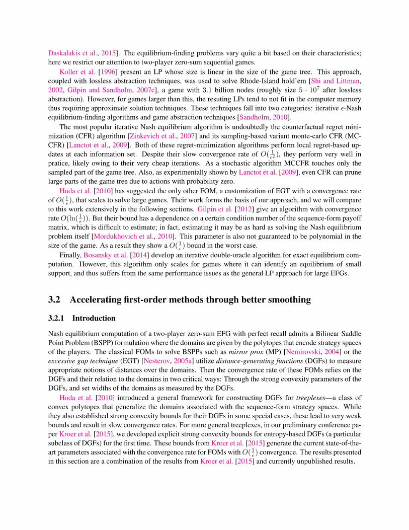
Nash equilibrium computation of a two-player zero-sum EFG with perfect recall admits a Bilinear SaddlePoint Problem (BSPP) formulation where the domains are given by the polytopes that encode strategy spacesof the players. The classical FOMs to solve BSPPs such as mirror prox (MP) [Nemirovski, 2004] or theexcessive gap technique (EGT) [Nesterov, 2005a] utilize distance-generating functions (DGFs) to measureappropriate notions of distances over the domains. Then the convergence rate of these FOMs relies on theDGFs and their relation to the domains in two critical ways: Through the strong convexity parameters of theDGFs, and set widths of the domains as measured by the DGFs.

Hoda et al. [2010] introduced a general framework for constructing DGFs for treeplexes—a class ofconvex polytopes that generalize the domains associated with the sequence-form strategy spaces. Whilethey also established strong convexity bounds for their DGFs in some special cases, these lead to very weakbounds and result in slow convergence rates. For more general treeplexes, in our preliminary conference pa-per Kroer et al. [2015], we developed explicit strong convexity bounds for entropy-based DGFs (a particularsubclass of DGFs) for the first time. These bounds from Kroer et al. [2015] generate the current state-of-the-art parameters associated with the convergence rate for FOMs withO(1

ε ) convergence. The results presentedin this section are a combination of the results from Kroer et al. [2015] and currently unpublished results.

In this section we construct a new weighting scheme for such entropy-based DGFs. This weightingscheme leads to new and improved bounds on the strong convexity parameter associated with generaltreeplex domains. In particular, our new bounds are first-of-their kind as they have no dependence onthe branching operation of the treeplex. Our strong convexity result allows us to improve the convergencerate of FOMs by a factor of O(bdd) (where b is the average branching factor for a player and d is the depthof the EFG) compared to the prior state-of-the-art results from Kroer et al. [2015]. Our bounds parallel thesimplex case for matrix games where the entropy function also achieves a logarithmic dependence on thedimension of the simplex domain. From a practical perspective, we emphasize that such an improvement ofthe strong convexity parameter is especially critical for stochastic FOMs, where it is not possible to speedup the search through line search techniques.

The top poker bots at the Annual Computer Poker Competition are created with the monte-carlo coun-terfactual regret minimization (MCCFR) algorithm [Lanctot et al., 2009], which is a sampling variant of thecounterfactual regret minimization algorithm (CFR) [Zinkevich et al., 2007, Brown et al., 2015]. Inspiredby this success, we also describe a family of sampling schemes that lead to unbiased gradient estimators forEFGs. Using these estimators and our DGF, we instantate the first stochastic FOM for EFGs.

Finally, we complement our theoretical results with numerical experiments to investigate the speed upof FOMs with convergence rate O(1

ε ) and compare the performance of these algorithms with the premierregret-based methods CFR and MCCFR. Our experiments show that FOMs are substantially faster thanCFR algorithms for medium-to-high-accuracy solutions. We also test the impact of stronger bounds onthe strong convexity parameter: we instantiate MP and EGT with the parameters developed in this paper,and compare the performance to the parameters developed in our preliminary conference version. Theseexperiments illustrate that, for both MP and EGT algorithms, the tighter parameters developed here lead tobetter practical convergence rate.

The rest of the section is organized as follows. We present the general class of problems that weaddress—bilinear saddle-point problems—and describes how they relate to EFGs in Section 3.2.2. ThenSection 3.2.3 describes our optimization setup. We introduce treeplexes, the class of convex polytopes thatdefine our domains of the optimization problems in Section 3.2.4. Our focus is on dilated entropy basedDGFs; we introduce these in Section 3.2.5 and present our main results—bounds on the associated strongconvexity parameter and treeplex diameter. In Section 3.2.6 we demonstrate the use of our results on in-stantiating MP algorithm. Section 3.2.7 introduces gradient estimators that enable the use of stochastic MP.We compare our approach with the current state-of-art in EFG solving and discuss the extent of theoreticalimprovements achievable via our approach in Section 3.2.8. Section 3.2.9 presents numerical experimentstesting the effect of various parameters on the performance of our approach as well as comparing the perfor-mance of our approach to CFR and MCCFR. We close with a summary of our results and a few compellingfurther research directions in Section 3.2.10.

3.2.2 Problem setup

Computing a Nash equilibrium in a two-player zero-sum EFG with perfect recall can be formulated as aBilinear Saddle Point Problem (BSPP):

minx∈X

maxy∈Y〈x,Ay〉 = max

y∈Yminx∈X〈x,Ay〉. (3.1)

This is known as the sequence-form formulation [Romanovskii, 1962, Koller et al., 1996, von Stengel, 1996].In this formulation, x and y correspond to the nonnegative strategy vectors for players 1 and 2 and the setsX ,Y are convex polyhedral reformulations of the sequential strategy space of these players. Here X ,Y

are defined by the constraints Ex = e, Fy = f , where each row of E,F encodes part of the sequentialnature of the strategy vectors, the right hand-side vectors e, f are |I1| , |I2|-dimensional vectors, and Ii isthe information sets for player i. For a complete treatment of this formulation, see von Stengel [1996].

Our theoretical developments mainly exploit the treeplex domain structure and are independent of otherstructural assumptions resulting from EFGs. Therefore, we describe our results for the general BSPPs. Wefollow the presentation and notation of Juditsky and Nemirovski [2011a,b] for BSPPs. For notation andpresentation of treeplex structure, we follow Hoda et al. [2010], Kroer et al. [2015].

Basic notation

We let 〈x, y〉 denote the standard inner product of vectors x, y. Given a vector x ∈ Rn, we let ‖x‖pdenote its `p norm given by ‖x‖p := (

∑ni=1 |xi|p)

1/p for p ∈ [1,∞) and ‖x‖∞ := maxi∈[n] |xi| forp =∞. Throughout this paper, we use Matlab notation to denote vector and matrices, i.e., [x; y] denotes theconcatenation of two column vectors x, y. For a given set Q, we let ri (Q) denote its relative interior. Givenn ∈ N, we denote the simplex ∆n := x ∈ Rn+ :

∑ni=1 xi = 1.

3.2.3 Optimization setup

In its most general form a BSPP is defined as

Opt := maxy∈Y

minx∈X

φ(x, y), (S)

where X ,Y are nonempty convex compact sets in Euclidean spaces Ex,Ey and φ(x, y) = υ + 〈a1, x〉 +〈a2, y〉 + 〈y,Ax〉. We let Z := X × Y; so φ(x, y) : Z → R. In the context of EFG solving, φ(x, y) issimply the inner product given in (3.1).

The BSPP (S) gives rise to two convex optimization problems that are dual to each other:

Opt(P ) = minx∈X [φ(x) := maxy∈Y φ(x, y)] (P )Opt(D) = maxy∈Y [φ(y) := minx∈X φ(x, y)] (D)

with Opt(P ) = Opt(D) = Opt. It is well known that the solutions to (S) — the saddle points of φ onX × Y — are exactly the pairs z = [x; y] comprised of optimal solutions to the problems (P ) and (D). Wequantify the accuracy of a candidate solution z = [x; y] with the saddle point residual

εsad(z) := φ(x)− φ(y) =[φ(x)− Opt(P )

]︸︷︷︸≥0

+[Opt(D)− φ(y)

]︸︷︷︸≥0

.

In the context of EFG, εsad(z) measures the proximity to being an ε-Nash equilibrium.The problems (P ) and (D) also give rise to the following variational inequality: find z∗ ∈ Z s.t.

〈F (z), z − z∗〉 ≥ 0 for all z ∈ Z, (3.2)

where F : Z 7→ Ex ×Ey is the affine monotone operator defined by

F (x, y) :=

[Fx(y) =

∂φ(x, y)

∂x;Fy(x) = −∂φ(x, y)

∂y

].

For EFG-solving purposes, F (x, y) corresponds to the map returning the gradients [Ay,−A>x] from (3.1).Then (3.2) states that for any other strategy pair z = [x, y], each player weakly prefers deviating to their partof z∗ = [x∗, y∗].

General framework for FOMs

Most FOMs capable of solving BSPP (S) are quite flexible in terms of adjusting to the geometry of theproblem characterized by the domains X ,Y of the BSPP (S). The following components are standard informing the setup for such FOMs:• Norm: ‖ · ‖ on the Euclidean space E where the domain Z = X × Y of (S) lives, along with its dual

norm ‖ζ‖∗ = max‖z‖≤1

〈ζ, z〉.

• Distance-Generating Function (DGF): A function ω(z) : Z → R, which is convex and continuous onZ , and admits a continuous selection of subgradients ω′(z) on the set Z := z ∈ Z : ∂ω(z) 6= ∅(here ∂ω(z) is a subdifferential of ω taken at z), and is strongly convex with modulus ϕ w.r.t. thenorm ‖ · ‖:

∀z′, z′′ ∈ Z : 〈ω′(z′)− ω′(z′′), z′ − z′′〉 ≥ ϕ‖z′ − z′′‖2. (3.3)

• Bregman distance: Vz(u) := ω(u)− ω(z)− 〈ω′(z), u− z〉 for all z ∈ Z and u ∈ Z .• Prox-mapping: Given a prox center z ∈ Z,

Proxz(ξ) := argminw∈Z

〈ξ, w〉+ Vz(w) : E→ Z.

For properly chosen stepsizes, the prox-mapping becomes a contraction. This is critical in the con-vergence analysis of FOMs. Furthermore, when the DGF is taken as the squared `2 norm, the proxmapping becomes the usual projection operation of the vector z − ξ onto Z .

• ω-center: zω := argminz∈Z

ω(z) ∈ Z of Z .

• Set width: Ω = Ωz := maxz∈Z

Vzω(z) ≤ maxz∈Z

ω(z)−minz∈Z

ω(z).

• Lipschitz constant: L of F from ‖ · ‖ to ‖ · ‖∗, satisfying ‖F (z)− F (z′)‖∗ ≤ L‖z − z′‖, ∀z, z′.In the standard customization of a FOM to solving a BSPP (S), we associate a norm ‖ · ‖x and a DGF

ωx(·) with the domain X , and similarly ‖ · ‖y, ωy(·) with the domain Y . Given two scalars αx, αy > 0, webuild the DGF ω(z) and ω-center zω for Z = X × Y as

ω(z) = αxωx(x) + αyωy(y) and zω = [xωx ; yωy ],

where ωx(·) and ωy(·) as well as xωx and yωy are customized based on the geometry of the domains X ,Y .In this construction, the flexibility in determining the scalars αx, αy > 0 is useful in optimizing the overallconvergence rate. Moreover, by letting ξ = [ξx; ξy] and z = [x; y], the prox mapping becomes decomposableas

Proxz(ξ) =

[Proxωxx

(ξxαx

); Proxωyy

(ξyαy

)],

where Proxωxx (·) and Proxωyy (·) are respectively prox mappings w.r.t. ωx(·) in domainX and ωy(·) in domainY .

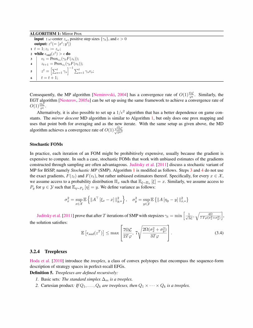
Based on this setup, we formally state the Mirror Prox (MP) algorithm in Algorithm 1.Suppose the step sizes in the MP algorithm satisfy γt = L−1. Then, at every iteration t ≥ 1 of the MP

algorithm, the corresponding solution zt = [xt; yt] satisfies xt ∈ X , yt ∈ Y , and

φ(xt)− φ(yt) = εsad(zt) ≤ ΩLϕt

.

ALGORITHM 1: Mirror Proxinput : ω-center zω , positive step sizes γt, and ε > 0output: zt(= [xt; yt])

1 t = 1; z1 := zω;2 while εsad(zt) > ε do3 vt = Proxzt(γtF (zt));4 zt+1 = Proxzt(γtF (vt));

5 zt =[∑t

s=1 γs

]−1∑ts=1 γsvs;

6 t = t+ 1;

Consequently, the MP algorithm [Nemirovski, 2004] has a convergence rate of O(1)ΩLϕε . Similarly, the

EGT algorithm [Nesterov, 2005a] can be set up using the same framework to achieve a convergence rate ofO(1)ΩL

ϕε .Alternatively, it is also possible to set up a 1/ε2 algorithm that has a better dependence on game con-

stants. The mirror descent MD algorithm is similar to Algorithm 1, but only does one prox mapping anduses that point both for averaging and as the new iterate. With the same setup as given above, the MDalgorithm achieves a convergence rate of O(1)

√ΩL√ϕε2

Stochastic FOMs

In practice, each iteration of an FOM might be prohibitively expensive, usually because the gradient isexpensive to compute. In such a case, stochastic FOMs that work with unbiased estimates of the gradientsconstructed through sampling are often advantageous. Juditsky et al. [2011] discuss a stochastic variant ofMP for BSSP, namely Stochastic MP (SMP). Algorithm 1 is modified as follows. Steps 3 and 4 do not usethe exact gradients, F (zt) and F (vt), but rather unbiased estimators thereof. Specifically, for every x ∈ X ,we assume access to a probability distribution Πx such that Eξ∼Πx [ξ] = x. Similarly, we assume access toPy for y ∈ Y such that Eη∼Py [η] = y. We define variance as follows:

σ2x = sup

x∈XE‖A> [ξx − x] ‖2y,∗

, σ2

y = supy∈Y

E‖A [ηy − y] ‖2x,∗

Juditsky et al. [2011] prove that after T iterations of SMP with stepsizes γt = min

[1√3L ,√

4Ω7Tϕ(σ2

x+σ2y)

],

the solution satisfies:

E[εsad(z

T )]≤ max

7ΩL2Tϕ

, 7

√2Ω(σ2

x + σ2y)

3Tϕ

. (3.4)

3.2.4 Treeplexes

Hoda et al. [2010] introduce the treeplex, a class of convex polytopes that encompass the sequence-formdescription of strategy spaces in perfect-recall EFGs.Definition 5. Treeplexes are defined recursively:

1. Basic sets: The standard simplex ∆m is a treeplex.2. Cartesian product: If Q1, . . . , Qk are treeplexes, then Q1 × · · · ×Qk is a treeplex.

3. Branching: Given a treeplex P ⊆ [0, 1]p, a collection of treeplexes Q = Q1, . . . , Qk where Qj ⊆[0, 1]nj , and l = l1, . . . , lk ⊆ 1, . . . , p, the set defined by

P l Q :=

(x, y1, . . . , yk) ∈ Rp+∑j nj : x ∈ P, y1 ∈ xl1 ·Q1, . . . , yk ∈ xlk ·Qk

is a treeplex. In this setup, we say xlj is the branching variable for the treeplex Qj .

A treeplex is a tree of simplices where children are connected to their parents through the branching op-eration. In the branching operation, the child simplex domain is scaled by the value of the parent branchingvariable. Understanding the treeplex structure is crucial because the proofs of our main results rely on in-duction over these structures. For EFGs, the simplices correspond to the information sets of a single playerand the whole treeplex represents that player’s strategy space. The branching operation has a sequentialinterpretation: The vector x represents the decision variables at certain stages, while the vectors yj representthe decision variables at the k potential following stages, depending on external outcomes. Here k ≤ p sincesome variables in x may not have subsequent decisions. For treeplexes, von Stengel [1996] has suggesteda polyhedral representation of the form Ex = e where the matrix E has its entries from −1, 0, 1 and thevector e has its entries in 0, 1.

For a treeplex Q, we denote by SQ the index set of the set of simplices contained in Q (in an EFG SQ isthe set of information sets belonging to the player). For each j ∈ SQ, the treeplex rooted at the j-th simplex∆j is referred to as Qj . Given vector q ∈ Q and simplex ∆j , we let Ij denote the set of indices of q thatcorrespond to the variables in ∆j and define qj to be the sub vector of q corresponding to the variables inIj . For each simplex ∆j and branch i ∈ Ij , the set Dij represents the set of indices of simplices reachedimmediately after ∆j by taking branch i (in an EFG Dij is the set of potential next-step information sets forthe player). Given a vector q ∈ Q, simplex ∆j , and index i ∈ Ij , each child simplex ∆k for every k ∈ Dijis scaled by qi. Conversely, for a given simplex ∆j , we let pj denote the index in q of the parent branchingvariable qpj that ∆j is scaled by. We use the convention that qpj = 1 ifQ is such that no branching operationprecedes ∆j . For each j ∈ SQ, dj is the maximum depth of the treeplex rooted at ∆j , that is, the maximumnumber of simplices reachable through a series of branching operations at ∆j . Then dQ gives the depth ofQ. We use bjQ to identify the number of branching operations preceding j-th simplex in Q.

Figure 3.1 illustrates an example treeplex Q. Q is constructed from nine two-to-three-dimensionalsimplices ∆1, . . . ,∆9. At level 1, we have taken the Cartesian product, denoted by ×, of the simplices ∆1

and ∆2. We have maximum depths d1 = 2, d2 = 1 beneath them. Since there are no preceding branchingoperations, the parent variables for these simplices ∆1 and ∆2 are qp1 = qp2 = 1. For ∆1, the correspondingset of indices in the vector q is I1 = 1, 2, while for ∆2 we have I2 = 3, 4, 5. At level 2, we have thesimplices ∆3, . . . ,∆7. The parent variable of ∆3 is qp3 = q1; therefore, ∆3 is scaled by the parent variableqp3 . Similarly, each of the simplices ∆3, . . . ,∆7 is scaled by their parent variables qpj that the branchingoperation was performed on. So on for ∆8 and ∆9 as well. The number of branching operations required toreach simplices ∆1,∆3 and ∆8 is b1Q = 0, b3Q = 1 and b8Q = 2, respectively.

Note that we allow more than two-way branches; hence our formulation follows that of Kroer et al.[2015] and differs from that of Hoda et al. [2010]. As discussed in Hoda et al. [2010], it is possible to modelsequence-form games by treeplexes that use only two-way branches. Yet, this can cause a large increase inthe depth of the treeplex, thus leading to significant degradation in the strong convexity parameter. Becausewe handle multi-way branches directly in our framework, our approach is more effective in taking intoaccount the structure of the sequence-form game and thereby resulting in better bounds on the associatedstrong convexity parameters and thus overall convergence rates.

∆1

q2 ·∆4

q8 q9

q1 ·∆3

q7 ·∆9

q19 q20

q7 ·∆8

q16q17

q18

q6 q7

q1 q2

∆2

q5 ·∆7

q14 q15

q4 ·∆6

q12 q13

q3 ·∆5

q10 q11

q3q4

q5

×

×

Figure 3.1: An example treeplex constructed from 9 simplices. Cartesian product operation is denoted by×.

Our analysis requires a measure of the size of a treeplex Q. Thus, we define

MQ := maxq∈Q‖q‖1. (3.5)

In the context of EFGs, suppose Q encodes player 1’s strategy space; then MQ is the maximum numberof information sets with nonzero probability of being reached when player 1 has to follow a pure strategywhile the other player may follow a mixed strategy. We also let

MQ,r := maxq∈Q

∑j∈SQ:bjQ≤r

‖qj‖1. (3.6)

Intuitively, MQ,r gives the maximum value of the `1 norm of any vector q ∈ Q after removing the variablescorresponding to simplices that are not within r branching operations of the root of Q.

3.2.5 Distance-generating functions with bounded strong convexity

In this section we introduce DGFs for domains with treeplex structures and establish their strong convexityparameters with respect to a given norm (see (3.3)).

The basic building block in our construction is the entropy DGF given by ωe(z) = −∑n

i=1 zi log(zi),for the simplex ∆n. It is well-known that ωe(·) is strongly convex with modulus 1 with respect to the`1 norm on ∆n (see Juditsky and Nemirovski [2011a]). We will show that a suitable modification of thisfunction achieves a desirable strong convexity parameter for the treeplex domain.

The treeplex structure is naturally related to the dilation operation [Hiriart-Urruty and Lemarechal,2001] defined as follows: Given a compact set K ⊆ Rd and a function f : K → R, we first define

K :=

(t, z) ∈ Rd+1 : t ∈ [0, 1] , z ∈ t ·K.

Definition 6. Given a function f(z), the dilation operation is the function f : K → R given by

f(z, t) =

t · f(z/t) if t > 0

0 if t = 0.

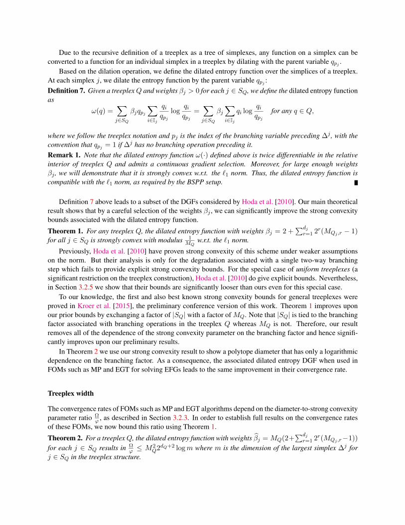
Due to the recursive definition of a treeplex as a tree of simplexes, any function on a simplex can beconverted to a function for an individual simplex in a treeplex by dilating with the parent variable qpj .

Based on the dilation operation, we define the dilated entropy function over the simplices of a treeplex.At each simplex j, we dilate the entropy function by the parent variable qpj :Definition 7. Given a treeplexQ and weights βj > 0 for each j ∈ SQ, we define the dilated entropy functionas

ω(q) =∑j∈SQ

βjqpj∑i∈Ij

qiqpj

logqiqpj

=∑j∈SQ

βj∑i∈Ij

qi logqiqpj

for any q ∈ Q,

where we follow the treeplex notation and pj is the index of the branching variable preceding ∆j , with theconvention that qpj = 1 if ∆j has no branching operation preceding it.Remark 1. Note that the dilated entropy function ω(·) defined above is twice differentiable in the relativeinterior of treeplex Q and admits a continuous gradient selection. Moreover, for large enough weightsβj , we will demonstrate that it is strongly convex w.r.t. the `1 norm. Thus, the dilated entropy function iscompatible with the `1 norm, as required by the BSPP setup.

Definition 7 above leads to a subset of the DGFs considered by Hoda et al. [2010]. Our main theoreticalresult shows that by a careful selection of the weights βj , we can significantly improve the strong convexitybounds associated with the dilated entropy function.

Theorem 1. For any treeplex Q, the dilated entropy function with weights βj = 2 +∑dj

r=1 2r(MQj ,r − 1)for all j ∈ SQ is strongly convex with modulus 1

MQw.r.t. the `1 norm.

Previously, Hoda et al. [2010] have proven strong convexity of this scheme under weaker assumptionson the norm. But their analysis is only for the degradation associated with a single two-way branchingstep which fails to provide explicit strong convexity bounds. For the special case of uniform treeplexes (asignificant restriction on the treeplex construction), Hoda et al. [2010] do give explicit bounds. Nevertheless,in Section 3.2.5 we show that their bounds are significantly looser than ours even for this special case.

To our knowledge, the first and also best known strong convexity bounds for general treeplexes wereproved in Kroer et al. [2015], the preliminary conference version of this work. Theorem 1 improves uponour prior bounds by exchanging a factor of |SQ| with a factor of MQ. Note that |SQ| is tied to the branchingfactor associated with branching operations in the treeplex Q whereas MQ is not. Therefore, our resultremoves all of the dependence of the strong convexity parameter on the branching factor and hence signifi-cantly improves upon our preliminary results.

In Theorem 2 we use our strong convexity result to show a polytope diameter that has only a logarithmicdependence on the branching factor. As a consequence, the associated dilated entropy DGF when used inFOMs such as MP and EGT for solving EFGs leads to the same improvement in their convergence rate.

Treeplex width

The convergence rates of FOMs such as MP and EGT algorithms depend on the diameter-to-strong convexityparameter ratio Ω

ϕ , as described in Section 3.2.3. In order to establish full results on the convergence ratesof these FOMs, we now bound this ratio using Theorem 1.

Theorem 2. For a treeplexQ, the dilated entropy function with weights βj = MQ(2+∑dj

r=1 2r(MQj ,r−1))

for each j ∈ SQ results in Ωϕ ≤ M2

Q2dQ+2 logm where m is the dimension of the largest simplex ∆j forj ∈ SQ in the treeplex structure.

3.2.6 Instantiating FOMs for extensive-form game solving

We now describe how to instantiate MP and MD for solving two-player zero-sum EFGs of the form givenin (3.1) for treeplex domains. The instantiation of EGT is similar. Below we state the customization of allthe definitions from Section 3.2.3 for our problem.

Let Z = X × Y be the treeplex corresponding to the cross product of the strategy spaces X ,Y forthe two players in (3.1) and m be the size of the largest simplex in this treeplex. Because X and Y aretreeplexes, it is immediately apparent that they are closed, convex, and bounded. We use the `1 norm onboth of the embedding spaces Ex,Ey; and as our DGF for Z compatible with `1 norm, we use the dilatedentropy DGF scaled with weights given in Theorem 2. Then Theorem 2 gives our bound on Ω

ϕ . Because thedual norm of `1 norm is the `∞ norm, an upper bound on the Lipschitz constant of our monotone operator,namely L, is given by:

L = max L1,L2 ,where

L1 = maxy∈Y

∣∣∣∣maxj

(Ay)j −minj

(Ay)j

∣∣∣∣ , L2 = maxx∈X

∣∣∣∣maxi

(A>x)i −mini

(A>x)i

∣∣∣∣ .Remark 2. Note that L is not at the scale of the maximum payoff difference in the original game. Thedifferences involved in L1,L2 are scaled by the probability of the observed nature outcomes on the path ofeach sequence. Thus, our Lipschitz constant L is exponentially smaller (in the number of observed naturesteps on the path to the maximizing sequence) than the maximum payoff difference in the original EFG.

Theorem 2 immediately leads to the following convergence rate result for MP or EGT equipped withdilated entropy DGFs to solve EFGs (and more generally BSPPs over treeplex domains).Theorem 3. Consider a BSPP over a treeplex domain Z . Suppose MP (or EGT) equipped with the dilatedentropy DGF with weights βj = 2 +

∑djr=1 2r(MZj ,r − 1) for all j ∈ SZ is used to solve the BSPP. Then

the convergence rate of this algorithm is

LM2Z 2dZ+2 logm

ε.

This rate is, to our knowledge, the state-of-the-art for FOMs with O(1/ε) convergence rate for EFGs.We can also instantiate MD, which has a better dependence on game constants, but sacrifices the linear

dependence on ε.Theorem 4. Consider a BSPP over a treeplex domain Z . Suppose MD equipped with the dilated entropyDGF with weights βj = 2 +

∑djr=1 2r(MZj ,r − 1) for all j ∈ SZ is used to solve the BSPP. Then the

convergence rate of this algorithm isLMZ 2dZ/2+1 logm

ε2.

For SMP we further need unbiased gradient estimators.

3.2.7 Sampling

We now introduce a broad class of unbiased gradient estimators for EFGs. We describe how to generate agradient estimate η of x>A given x ∈ X , that is, the gradient for player 2. Given y ∈ Y , the estimate ξ ofA>y is generated analogously. This class explicitly uses the tree structure representation of EFGs, so we

introduce some notation for it. We define H to be the set of nodes (or equivalently, histories) in the gametree. For any node h, we define A(h) to be the set of actions available at h. The node reached by takingaction a ∈ A(h) at h is denoted by h[a]. We let ph,x be the probability distribution over actions A(h) givenby the current iterate x. If h is a chance node, x has no effect on the distribution. We let u2(h) be the utilityof player 2 for reaching a terminal node h, and ηh be the index in η corresponding to a given terminal nodeh.

An EFG gradient estimator is defined by a sampling-description function C : H → N ∪ all, whereC(h) gives the number of samples drawn at the node h ∈ H . The estimate η of x>A is then generated usingthe following recursive sampling scheme:

Sample(h, τ) :

if h is a terminal node : ηh = τ · u2(h)

else if h belongs to player 2: ∀a ∈ A(h) : Sample(h[a], τ)

else if C(h) = all: ∀a ∈ A(h) : Sample(h[a], ph,x(a) · τ)

else:

Draw

a1, . . . , aC(h)

∼ ph,x,

∀j = 1, . . . , C(h) : Sample(h[aj ], τ · 1C(h))

.

Sampling is initiated with h = r, τ = 1, where r is the root node of the game tree. From the definition ofthis sampling scheme, it is clear that the expected value of any EFG estimator is exactly x>A as desired. Itis possible to generalize this class to sample A(h) at nodes h belonging to player 2 as well.

Lanctot et al. [2009] introduced several unbiased sampling schemes for EFGs. These correspond tocertain specializations of our general sampling scheme. Chance sampling, Cc(h), is where a single sampleis drawn if the node is a nature node, and otherwise all actions are chosen. This corresponds to the followingEFG estimator:

Cc(h) =

1 if h is a chance nodeall else

.

In external sampling, Ce(h), a single sample is drawn for the nodes that do not belong to the current player.Hence, when we estimate x>A, we get Ce(h) = 1.

In our experiments, for a given positive integer k, we focus on the following estimator

Cc,k(h) =

k if h is a chance nodeall else

. (3.7)

We now provide a simple upper bound for the variance of this class of gradient estimators. We will needthe maximum payoff difference for Player 2 in the EFG, which we denote by Γ2 = maxh,h′ u2(h)−u2(h′).An analogous theorem holds for σ2

y .Theorem 5. Any gradient estimator C : H → N ∪ all, has variance at most σ2

x ≤ Γ22.

This result immediately leads to the following first-of-its-kind bound on the convergence rate of astochastic FOM for EFG solving:Theorem 6. Consider a BSPP over a treeplex domain Z . Suppose SMP equipped with the dilated entropyDGF with weights βj = 2 +

∑djr=1 2r(MZj ,r − 1) for all j ∈ SZ and any gradient estimator C is used to

solve the BSPP. Using stepsizes γt = min

[1√3L ,

√4M2Z2dZ+2 logm

7T (Γ21+Γ2

2)

], the expected convergence rate of this

algorithm is

E[εsad(z

T )]≤ max

[7LM2

Z2dZ+2 logm

2T, 7

√2M2Z2dZ+2 logm(Γ2

1 + Γ22)

3T

]. (3.8)

3.2.8 Discussion of theoretical improvements

We first discuss the theoretical improvement in convergence rate originating from our new strong convexityand set width parameter bounds for FOMs achieving O(1

ε ) rate and then elaborate on how our convergencerate result is positioned with respect to other equilibrium-finding algorithms from the literature.

Improvement on strong convexity and set width parameter bounds

The ratio Ωϕ of set diameter over the strong convexity parameter is important for FOMs that rely on a prox

function, such as Nesterov’s EGT, MP, and SMP.Compared to the rate obtained in our preliminary conference version [Kroer et al., 2015], we get the

following improvement: Assuming that the number of actions available at each information set is on averagea, our bound improves the convergence rate of [Kroer et al., 2015] by a factor of O(dZ · adZ ).

As mentioned previously, Hoda et al. [2010] proved only explicit bounds for the special case of uniformtreeplexes that are constructed as follows: 1) A base treeplex Q along with a subset of b indices from it forbranching operations is chosen. 2) At each depth d, a Cartesian product operation of size k is applied. 3)Each element in a Cartesian product is an instance of the base treeplex with a size b branching operationleading to depth d − 1 uniform treeplexes constructed in the same way. Given bounds Ωb, ϕb for the basetreeplex, the bound of Hoda et al. [2010] for a uniform treeplex with d uniform treeplex levels (note that thetotal depth of the constructed treeplex is d · dQ, where dQ is the depth of the base treeplex Q) is

Ω

ϕ≤ O

(b2d−2k2d+2d2M2

Qb

Ωb

ϕb

).

Then when the base treeplex is a simplex of dimension m, their bound for the dilated entropy on a uniformtreeplex Z becomes

Ω

ϕ≤ O

(|SZ |2 d2

Z logm).

Even for the special case of a uniform treeplex with a base simplex, comparing Theorem 2 to their bound, wesee that our general bound improves the associated constants by exchanging O(|SQ|2 d2

Z) with O(M2Q2dZ ).

Since MQ does not depend on the branching operation in the treeplex, whereas |SQ| does, these are also thefirst bounds to remove any dependence on the branching operation.

A more intuitive bound on CFR convergence rate

The CFR literature has had several papers improving previous bounds on the convergence rate of the algo-rithm [Zinkevich et al., 2007, Lanctot et al., 2009, Burch et al., 2012]. The most recent such result shows abound of [Burch et al., 2012]:

∆iMi(σ∗i )√|Ai|√

T

where ∆i is the maximum payoff difference in the game, andMi(σ∗i ) is equal to

∑B∈Bi π

σ∗i (B)

√|B|. This

bound is somewhat difficult to compare to the original CFR bound as well as our results. In this section weexpress this bound in terms of a uniform game where players 1, 2, and nature alternate d times and have thesame number of actions |A1| = |A2| = |A0| = b. Note that this corresponds to each player’s strategy spacebeing a treeplex with depth d, branching operations of size b, and Cartesian product operations of size k.

Let player i be the player that goes second. For such a game, we get∑B∈Bi

πσ∗i (B)

√|B| =

∑B∈Bi

πσ∗i (B)

√k

=∑B∈Bi

πσ∗i (B)

√k =

∑B∈Bi

1

bd−dB

√k

=d∑

h=1

∑B∈Bi,dB=h

1

bd−h

√k =

d∑h=1

(bk)d−h1

bd−h

√k

=d∑

h=1

kd−h√k =√kkh − 1

k − 1,

As can be seen this value is essentially the same as MQ, i.e. the maximum value of the l1 norm over Q.

Improvements in extensive-form game convergence rate

CFR, EGT, MP, and SMP all need to keep track of a constant number of current and/or average iterates, sothe memory usage of all four algorithms is of the same order: when gradients are computed using an iterativeapproach as opposed to storing matrices or matrix decompositions, each algorithm requires a constant timesthe number of sequences in the sequence-form representation. Therefore, we compare mainly the numberof iterations required by each algorithm.

Theorem 2 establishes the best known results on strong convexity parameter and set width of prox func-tions based on dilated entropy DGF over treeplex domains; and consequently, Theorems 3 and 6 establishthe best known convergence results for all FOMs based on dilated entropy DGF such as MP, MD, SMP, andEGT algorithms.

In comparison to such FOMs, CFR and its stochastic counterpart MCCFR are the most popular algo-rithms for practical large-scale equilibrium finding. CFR has a O( 1

ε2) convergence rate; but its dependence

on the number of information sets is only linear (and sometimes sublinear [Lanctot et al., 2009]). Since ourresults have a quadratic dependence on M2

Q, CFR has a better dependence on game constants and can bemore attractive for obtaining low-quality solutions quickly for games with many information sets. MCCFRhas a similar convergence rate [Lanctot et al., 2009]. When we apply SMP with our results, we achieve anexpected convergence rate of O( 1

ε2), but with only a square root dependence on the ratio Ω

ϕ in (3.4). Despitetheir slower convergence rates, it is important to note that both SMP and MCCFR algorithms have muchcheaper iterations compared to the deterministic algorithms.

On a separate note, Gilpin et al. [2012] give an equilibrium-finding algorithm presented asO(ln(1ε )); but

this form of their bound has a dependence on a certain condition number of the A matrix. Specifically, their

iteration bound for sequential games is O(‖A‖2,2·ln(‖A‖2,2/ε)·

√D

δ(A) ), where δ(A) is the condition number of A,

‖A‖2,2 = supx 6=0‖Ax‖2‖x‖2 is the Euclidean matrix norm, and D = maxx,x∈X ,y,y∈Y ‖(x, y)− (x, y)‖22. Unfor-

tunately, the condition number is only shown to be finite for these games. Without any such unknown quan-tities based on condition numbers, Gilpin et al. [2012] establish an upper bound ofO(

‖A‖2,2·Dε ) convergence

rate. This algorithm, despite having the same dependence on ε as ours in its convergence rate, i.e., O(1ε ),

suffers from worse constants. In particular, there exist matrices such that ‖A‖2,2 =√‖A‖1,∞‖A‖∞,1,

where ‖A‖1,∞ and ‖A‖∞,1 correspond to matrix norms given by the maximum absolute column and rowsums, respectively. Then together with the value of D, this leads to a cubic dependence on the dimension of

Q. For games where the players have roughly equal-size strategy spaces, this is equivalent to a constant ofO(M4

Q) as opposed to our constant of O(M2Q).

3.2.9 Numerical experiments

We carry out numerical experiments to investigate the practical performance of several iterative methodsused in conjunction with EFGs and demonstrate the practical impact of our theoretical results. Specifically,we consider first-order methods EGT, MP, SMP together with regret-based algorithms CFR and MCCFR.For EGT, MP, and SMP we employ the dilated entropy DGF with weights chosen according to Theorem 2.To enhance the practical performance of EGT, we employ the balancing heuristic described by Hoda et al.[2010]. We run CFR with pruning, which was shown to improve its performance Lanctot et al. [2009]. ForMCCFR and SMP we tested 4 different EFG gradient estimators: Cc,1, Cc,5, Cc,10, Cc,20 (c.f. (3.7)). In ourexperiments we report only the results of the best estimater for each: MCCFR was best with Cc,1 while SMPwas best with Cc,20. For SMP, rather than employing the very small fixed stepsize given in (3.4), we use adecreasing stepsize that approaches this value from above.

We test these algorithms on a scaled up variant of the poker game Leduc holdem [Southey et al., 2005], abenchmark problem in the imperfect-information game-solving community. In our version, the deck consistsof k pairs of cards 1 . . . k, for a total deck size of 2k. Each player initially pays one chip to the pot, and isdealt a single private card. After a round of betting, a community card is dealt face up. After a subsequentround of betting, if neither player has folded, both players reveal their private cards. If either player pairstheir card with the community card they win the pot. Otherwise, the player with the highest private cardwins. In the event both players have the same private card, they draw and split the pot.

The results are shown in Figure 3.2. Each graph is a loglog plot that shows the results for a particularinstance of Leduc with 6, 10, 16 and 30 card decks, respectively. For each graph, we show the performanceof all five algorithms, with the x-axis showing the number of nodes in the game tree touched and the y-axisshowing the maximum regret over the two players. In these plots, we use the number of nodes touched inorder to account for the pruning in the CFR version that we run together with the effect of other constantssuch as the fact that the algorithms perform different numbers of tree traversals per iteration (for example,MP and SMP require two prox function applications). In line with what the theory predicts, FOMs withconvergence rate O(1

ε ) such as EGT and MP convergence faster despite the fact that they initially start outslower. These results suggest that they might be better suited for medium-to-high-precision equilibriumcomputation and smaller size instances. SMP does not perform as well on smaller instances; but its per-formance improves as the instances get larger. For example, while SMP is initially preferable to EGT andMP for the 30-card game, its performance deteriorates as the accuracy needed increases. We attribute thisbehavior of SMP to the small stepsizes required by SMP.

In our preliminary experiments, we observed that both MP and SMP are very sensitive to parameterselection. Nevertheless, we did not perform much engineering of the parameters of these algorithms in ourexperiments. This suggests the possibility of improving their practical performance with a more thoroughexperimental investigation which we leave as future work.

We also investigate the practical impact of applying the weights used in Theorem 3 (henceforth re-ferred to as new weights), rather than the weights proposed in the preliminary conference version of thispaper Kroer et al. [2015] (henceforth referred to as old weights). Figure 3.3 shows the result of runningEGT and MP with the old and the new weights. As the stepsize parameter for MP (γ) and smoothing pa-rameter for EGT (µ) required by the theory were found to be too conservative, in the left figure, we showthe results after tuning these parameters for the corresponding algorithms to yield the best results for eachweight vectors. The theory suggests the same stepsize and smoothing values for both old and new weights.

103 104 105 106 107 108 10910−5

10−4

10−3

10−2

10−1

100

Leduc 6 card

EGT

MP

CFR

MCCFR

SMP

103 104 105 106 107 108 10910−4

10−3

10−2

10−1

100

Leduc 10 card

EGT

MP

CFR

MCCFR

SMP

103 104 105 106 107 108 10910−3

10−2

10−1

100

Leduc 16 card

EGT

MP

CFR

MCCFR

SMP

103 104 105 106 107 108 10910−3

10−2

10−1

100

Leduc 30 card

EGT

MP

CFR

MCCFR

SMP

Figure 3.2: Regret as a function of the number of nodes touched in four different variants of Leduc holdemfor the CFR, MCCFR, EGT, MP, and SMP algorithms.

101 102 103 10410−4

10−3

10−2

10−1

100

Leduc 6 card, EGT and MP, best weights

MP old, γ = 0.0002

MP new, γ = 0.0004

EGT old, µ = 0.0001

EGT new, µ = 0.001

101 102 103 10410−3

10−2

10−1

100

Leduc 6 card, EGT, same weights

EGT old, µ = 0.005

EGT new, µ = 0.005

Figure 3.3: Regret as a function of the number of iterations for MP and EGT. Both axes are on a log scale.Throughout old corresponds to the weights from Kroer et al. [2015] and new corresponds to theweights from Theorem 3. The left plot shows MP with the old and new weights (γ denotes thestepsize) and EGT with the old and new weights (µ denotes the initial smoothing parameter).The right plot shows EGT with old and new weights using a fixed smoothing parameter µ.

Regardless of this, we noticed that the old weights are more sensitive to tuning and have smaller stepsizeand smoothing values. The right figure shows results for EGT when applying a single smoothing parameterto both the old and new weights. We observe that the positive impact of our new weighting scheme is morepronounced for MP. MP performs significantly better with the new stepsizes, with about an order of mag-nitude improvement. EGT also performs better with the new weights, both when using the same µ (on theright), and when using individually tuned µ (on the left).

3.2.10 Conclusions

We have investigated FOMs for computing Nash equilibria in two-player zero-sum perfect-recall EFGs. Onthe theoretical side, we analyzed the strong convexity properties of the dilated entropy DGF over treeplexes.By introducing specific weights that are tied to the structure of the treeplex, we improved prior results ontreeplex diameter from O(|SQ|2d2

Z) to O(M2Q2dZ ), thereby removing all dependence on branching from

the Cartesian product operator in the treeplex definition. Our results generalize to any treeplex, whereasthe prior results were for only uniform treeplexes, a significant restriction. These results lead to significantimprovements in the convergence rates of many FOMs that can be equipped with dilated entropy DGFsand used for EFG solving including but not limited to EGT, MP, and SMP. Finally, we designed a class ofsampling schemes for gradient estimation, generalizing prior schemes considered for MCCFR.

We numerically investigated the performance of EGT, MP, SMP, CFR, and MCCFR. For moderately-sized games, our experiments indicate that FOMs such as MP or EGT with the dilated entropy DGF havebetter practical, as well as theoretical, convergence rate than the current common practice of using CFRalgorithms. However, there is a cross-over point at which FOMs beat CFR. Our experiments demonstratedthat the cross-over point required more iterations to reach as the games got larger. This begs the questionof to what extent the improvements resulting from our approach can make FOMs competitive with CFRfor very large games where exact solutions are not computed. Because both MP and SMP are much morecustomizable than the other FOMs and here we only considered their basic variants, a compelling researchdirection is to investigate various strategies for step sizes and parameter choices for MP and SMP and seetheir impact on the practical performance of these algorithms and how they compare against EGT.

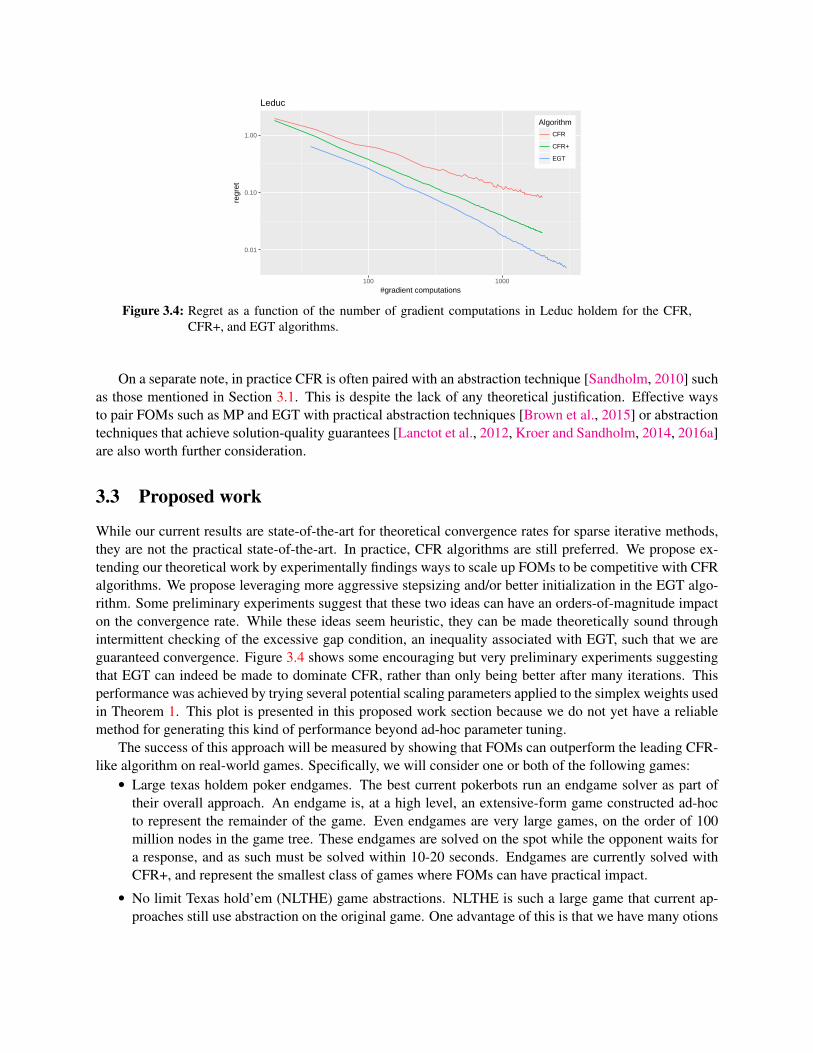
0.01

0.10

1.00

100 1000

#gradient computations

regr

et

Algorithm

CFR

CFR+

EGT

Leduc

Figure 3.4: Regret as a function of the number of gradient computations in Leduc holdem for the CFR,CFR+, and EGT algorithms.

On a separate note, in practice CFR is often paired with an abstraction technique [Sandholm, 2010] suchas those mentioned in Section 3.1. This is despite the lack of any theoretical justification. Effective waysto pair FOMs such as MP and EGT with practical abstraction techniques [Brown et al., 2015] or abstractiontechniques that achieve solution-quality guarantees [Lanctot et al., 2012, Kroer and Sandholm, 2014, 2016a]are also worth further consideration.

3.3 Proposed work

While our current results are state-of-the-art for theoretical convergence rates for sparse iterative methods,they are not the practical state-of-the-art. In practice, CFR algorithms are still preferred. We propose ex-tending our theoretical work by experimentally findings ways to scale up FOMs to be competitive with CFRalgorithms. We propose leveraging more aggressive stepsizing and/or better initialization in the EGT algo-rithm. Some preliminary experiments suggest that these two ideas can have an orders-of-magnitude impacton the convergence rate. While these ideas seem heuristic, they can be made theoretically sound throughintermittent checking of the excessive gap condition, an inequality associated with EGT, such that we areguaranteed convergence. Figure 3.4 shows some encouraging but very preliminary experiments suggestingthat EGT can indeed be made to dominate CFR, rather than only being better after many iterations. Thisperformance was achieved by trying several potential scaling parameters applied to the simplex weights usedin Theorem 1. This plot is presented in this proposed work section because we do not yet have a reliablemethod for generating this kind of performance beyond ad-hoc parameter tuning.

The success of this approach will be measured by showing that FOMs can outperform the leading CFR-like algorithm on real-world games. Specifically, we will consider one or both of the following games:• Large texas holdem poker endgames. The best current pokerbots run an endgame solver as part of

their overall approach. An endgame is, at a high level, an extensive-form game constructed ad-hocto represent the remainder of the game. Even endgames are very large games, on the order of 100million nodes in the game tree. These endgames are solved on the spot while the opponent waits fora response, and as such must be solved within 10-20 seconds. Endgames are currently solved withCFR+, and represent the smallest class of games where FOMs can have practical impact.

• No limit Texas hold’em (NLTHE) game abstractions. NLTHE is such a large game that current ap-proaches still use abstraction on the original game. One advantage of this is that we have many otions

for the exact kind of abstraction we want to solve, By increasing the scalability of equilibrium al-gorithms, we can enable the solution of larger game abstractions. NLTHE is the current frontier oflarge-scale EFG solving, where many of the state-of-the-art contemporary bots are more exploitablethan always folding [Lisy and Bowling, 2017].

Theoretically, we propose extending our results by developing corresponding lower bounds on the con-vergence rates achievable with the class of entropy-based smoothing functions we consider. Furthermore,we propose showing corresponding upper and/or lower bounds on the convergence rate achievable withdilation-based l2 smoothing. Ideally, this will allow us to show that entropy-based smoothing is theoret-ically superior to l2 smoothing for EFGs. This would complement experimental results from Hoda et al.[2010], which found entropy smoothing to be superior, and parallel the simplex case, where the entropyDGF is known to be superior.

Finally, we propose the development of sparse iterative methods for computing Nash equilibrium re-finements. In the case of zero-sum games, polynomial time algorithms are known for refinements suchas normal-form proper and quasi-perfect equilibria [Miltersen and Sørensen, 2008, 2010, Farina and Gatti,2017]. However, these algorithms rely on solving one or more linear programs which are modifications tothe sequence-form LP of von Stengel [1996]. This leads to LPs whose size is linear in the size of the gametree. As with regular Nash equilibrium computation, such LP formulations are not practical for large-scalegames. Instead, we propose leveraging a perturbed sequence-form polytope (such as that of Miltersen andSørensen [2010]) in the standard bilinear saddle-point formulation, and then focus on solving this perturbedsaddle-point problem directly. For a small enough perturbation, solving this perturbed problem should leadto an approximate equilibrium refinement. We propose combining our results from this chapter with a lin-early perturbed dilated entropy DGF, and then applying solvers such as EGT or MP to the computation ofapproximate quasi-perfect equilibria or extensive-form perfect equilibria.

Chapter 4

Abstraction for large games

Initially, game abstractions were created by hand, using domain dependent knowledge [Shi and Littman,2002, Billings et al., 2003]. More recently, automated abstraction has taken over [Gilpin and Sandholm,2006, 2007c, Zinkevich et al., 2007]. This has typically been used for information abstraction, whereasaction abstraction is still largely done by hand [Gilpin et al., 2008, Schnizlein et al., 2009]. Recently,automated action abstraction approaches have also started to emerge [Hawkin et al., 2011, 2012, Sandholmand Singh, 2012, Brown and Sandholm, 2014, 2015].

Ideally, abstraction would be performed in a lossless way, such that implementing an equilibrium fromthe abstract game results in an equilibrium in the full game. Abstraction techniques for this were introducedby Gilpin and Sandholm [2007c] for a subclass of games called game of ordered signals. Unfortunately,lossless abstraction often leads to games that are still too large to solve. Thus, we must turn to lossy ab-straction. However, significant abstraction pathologies (nonmonotonicities) have been shown in games thatcannot exist in single-agent settings: if an abstraction is refined, the equilibrium strategy from that newabstraction can actually be worse in the original game than the equilibrium strategy from a coarser abstrac-tion Waugh et al. [2009a]! Until recently, all lossy abstraction techniques for general games of imperfectinformation were without any solution quality bounds. Basilico and Gatti [2011] give bounds for the specialgame class Patrolling Security Games. Johanson et al. [2013] provide computational methods for evaluatingthe quality of a given abstraction via computing a best response in the full game after the fact. Lanctotet al. [2012] present regret bounds for strategies with low immediate regret computed in imperfect recallabstractions, with their result also extending to perfect-recall abstractions. Their result depends on the coun-terfactual regret minimization (CFR) algorithm being used for equilibrium computation in the abstraction,and focuses on abstraction via information coarsening, thus allowing neither action abstraction nor reductionof the size of the game tree in terms of nodes. Waugh et al. [2015] and Brown and Sandholm [2015] developiterative abstraction-refinement schemes that converge to a Nash equilibrium in the limit, but do not givebounds when an abstraction of the game is solved. Sandholm and Singh [2012] provide lossy abstractionalgorithms with bounds for stochastic games. They leave as an open problem whether similar bounds canbe achieved for extensive-form games. A key complication keeping the analysis in their paper from directlyextending to extensive-form games is information sets. In stochastic games, once the opponent strategiesare fixed, the best response analysis can be approached on a node-by-node basis. With information sets thisbecomes much more complex, as strategies have to be evaluated not only according to how they perform ata given node, but also how they perform according to the distribution of nodes in the information set.

This chapter develops the first algorithm-agnostic theoretical bounds on solution quality for (possiblyapproximate) Nash equilibria computed in abstractions of EFGs rather than the full game. In addition, the

28

bounds we develop (both for perfect and imperfect-recall abstractions) are exponentially stronger than theonly prior (algorithm specific) bounds for EFGs [Lanctot et al., 2012].

4.1 Perfect-recall abstraction

4.1.1 Introduction

This section develops the first bounds on lossy abstraction in general perfect-recall extensive-form games.These results are independent of the equilibrium computation approach, and allow both information coars-ening and removal of nodes and actions to make the game tree smaller.

To achieve these more general results, we introduce several new analysis tools:1. Most importantly, much of our analysis operates on a per information set basis, which fundamentally

changes how the analysis can be performed.

2. To enable high expressiveness in the types of abstractions that can be computed, our mappings be-tween real and abstract games are not all surjective functions.

3. We introduce a stricter notion of strategy mapping, called undivided lifted strategies.

4. We introduce a new solution concept, self-trembling equilibrium, the concept of which is used in ouranalysis to achieve bounds for general Nash equilibria (defined in Section 2.3).

5. We introduce several new notions of error in abstractions that are used to characterize our bounds.As a special case, our results generalize the results of Sandholm and Singh [2012], since any DAG-

structured stochastic game can be converted to an extensive form game. We also tighten the bound givenin their paper. Since our results apply to general Nash equilibria, as well as subgame-perfect equilibria, wealso generalize the set of equilibrium concepts that the analysis applies to; theirs was for subgame-perfectequilibrium.

Our framework is the first general theoretical framework for reasoning about quality of equilibria com-puted in abstract games. The only prior work [Gilpin and Sandholm, 2007c] is for a very restricted settingthat closely resembles poker games, and only concerns lossless abstraction. In contrast, our results apply toall extensive-form games of perfect recall, and can be used to reason about both lossless and lossy abstrac-tion. Further, we show that, even in the restricted setting considered in their paper, our framework can findlossless abstractions that theirs cannot.

We also present several new algorithmic characterizations and algorithms for building abstractions thatminimize our bounds. We show several hardness results related to computing abstractions on a level-by-levelbasis, and show how only considering level-by-level abstraction can lead to not finding the smallest, or any,lossless abstractions. Motivated by these results, we develop the first abstraction algorithm with boundedloss, which operates on all levels of the tree at once. We then present experimental results, where we applyour algorithm to a relatively simple poker game. Finally, we discuss additional results, connections to otherabstraction approaches, and directions for future research.

4.1.2 Framework

We will consider two extensive form games, the original game Γ and the abstract game Γ′. Both gameshave the same set of players N . The same elements are defined for Γ′, except each one is denoted by aprime superscript. For example, the node space for Γ′ is denoted by S′. The value for player i at leaf nodez′ ∈ Z ′ in Γ′ is denoted ui(z′). We define the largest utility at any leaf node in the abstract game to beW = maxi maxz′∈Z′ ui(z

′), which will be useful later.

We will use W σ′i : S ′i → R and W σ′

i : I ′i → R to denote the value functions for the abstract gameΓ′ (completely analogous to the value functions for the original game defined in Section 2.2). Thus, byProposition 1 we can write the value function for the abstract game as

W σ′i (I ′) =

∑a′∈AI′

σ′(I ′, a′)∑I′∈Da′

I′

πσ′−i(I

′)

πσ′−i(I

′)W σ′i (I ′).

Abstraction functions

We define an information set abstraction function f : I → I ′ which maps from original information setsto abstract information sets. Similarly, h : S → S ′ is a node abstraction function that maps from originalnodes to abstract nodes. Finally, g : A → A′ is an action abstraction function that maps from originalactions to abstract actions. All three functions are surjections, so that the game Γ′ is no bigger than Γ, andideally significantly smaller. We define f−1 : I ′ → I to be the set-valued inverse of the information setabstraction function. For a given I ′, f−1(I ′) returns all information sets that map to I ′. We define h−1 andg−1 similarly. We also define the function h−1

I : S ′ → S which for given I, s′ ∈ f(I) returns h−1(s′) ∩ I ,the subset of nodes in I that map to s′. Similarly, we define, h−1

Ps : S ′ → S which for a given s, s′ returnsh−1(s′) ∩ Ps, where Ps is the set of all ancestors and descendants of s.

We require that for any two actions that map to the same abstract action, the two nodes respectivelyreached by performing the actions at a given node map to the same abstract node. Formally, for all s ∈ S, ifg(a1) = g(a2) for a1, a2 ∈ As, then h(tsa1) = h(tsa2), where tsa is the node reached by performing action aat state s, as defined above.

As with prior abstraction approaches, these abstraction functions allow us to map a larger game onto asmaller game, through many-to-one mapping of nodes. We now present a novel approach for mapping nodesone-to-many. This leads to a larger set of valid abstractions, thereby sometimes allowing either smallerabstractions for a given bound, or the same size abstraction with a smaller bound. We call this “multi-mapping”. An example where it is useful is given in Figure 4.1. In this game, nature starts out choosingamong four actions. Player one then has two information sets, one for when either of the two leftmostnature actions were chosen, and one for when either of the two rightmost nature actions were chosen. Ifplayer 1 goes left at any node, player 2 then has two information sets. Player 2 can also only distinguishbetween nature’s actions in sets of two, but different sets than player 1. In this game, we can losslessly treatplayer 2’s information sets 2A, 2C and 2B, 2D as one big information set, since there is a mapping ofactions at 2A to actions at 2B such that the utilities for Player 2 are the same, and similarly for 2C and 2D.However, we need to formalize the notion that 2A is similar to 2B without merging the nodes, as they arenot similar for Player 1. In mapping the smaller information set 2A, 2C onto the abstract information set2A, 2C, 2B, 2D, we wish to specify that 2A is represented by the two nodes 2A and 2B. 1

We will now incorporate “multi-mapping” into the abstraction framework. To our knowledge, we arethe first to allow for such abstraction. We define a mapping function φ : Sφ → 2S

′which maps from a

subset Sφ ⊂ S of the original nodes to the powerset 2S′

of the abstract nodes. For all information sets I , wedefine the sets Iφ, I¬φ, the partition of I into two sets such that s ∈ Sφ for s ∈ Iφ and s /∈ Sφ for s ∈ I¬φ.

Since in our abstraction framework we are allowing “multi-mapping” (one original node mapped to mul-tiple abstract nodes), we have to ensure that all those abstract nodes are similar (in terms of their dependence

1This does not create a smaller abstraction in terms of the tree size, but it decreases the number of information sets. This isrelevant to equilibrium-finding algorithms, such as CFR, whose complexity depends on the number of information sets rather thanthe number of nodes in the game tree. A similar notion of abstraction was introduced by Lanctot et al. [2012].

N

P1

2A

0,1 2,0

0,1

P1

2B

0,1 0,0

0,0

P1

2C

12,0 2,1

0,10

P1

2D

0,0 0,1

0,1

Figure 4.1: Extensive form game, with nature playing first, picking among four outcomes uniformly atrandom. The next level, with nodes denoted P1, belongs to player 1, and the last level ofinternal nodes named 2A-2D belong to player 2.

on the other players). Specifically, we require the following constraints for each information set I such thatIφ > 0.

1. If an abstract node s′ ∈ f(I) is part of φ(s) for some s ∈ Iφ, then no other nodes in I can map to s′.

2. For all nodes s and pairs of nodes s′1, s′2 ∈ φ(s) at level k, each level l ∈ H−0, l > k, the edges on

the respective paths to s′1, s′2 must be in an information set together, and belong to the same action, or

both be in information sets with a single action.

3. For all abstract nodes s′ ∈ φ(s), we require that the subtree rooted at s also maps onto the subtreerooted at s′. For all such pairs of nodes, we define a surjective function φs,s′ , completely analogousto the function h, defining this mapping.

4. For all descendants s of s and pairs of nodes s′1, s′2 ∈ φ(s), φs,s′1(s) must be in the same information

set as φs,s′2(s).The example presented above can be described in terms of our φ function: φ(2A) = 2A, 2B, φ(2B) =

2A, 2B, φ(2C) = 2C, 2D, φ(2D) = 2C, 2D. Since the children of these nodes are all leaf nodes,we need not define the subtree mapping functions φ2A,2B, φ2C,2B .

Mapping behavioral strategies from the abstract game back to the original game

When computing a strategy profile σ′ in Γ′, we need some notion of how to interpret this profile in Γ. Herewe introduce two classes of mappings from abstract strategies to real strategies. First, we present the naturalextension of lifted strategies introduced by Sandholm and Singh [2012] to extensive-form games. In thisdefinition, a valid mapping σ↑σ

′is any strategy profile such that for each information set I and abstract

action a′ ∈ Af(I), the probability σ′(f(I), a′) of selecting that abstract action is divided any way across theactions g−1(a′) ∩ I .Definition 8. (Strategy lifting) Given an abstract game Γ′ and a strategy profile σ′, a lifted strategy for Γ isa strategy profile σ↑σ

′such that for all I , all a′ ∈ Af(I):

∑a∈g−1(a′) σ

↑σ′(I, a) = σ′(f(I), a′).For our game-theoretic results, we require a stronger notion of similarity in the mapping. We introduce

undivided lifted strategies, a refinement of lifted strategies. In addition to the lifted strategy constraint, werequire that the probability distribution over nodes in an information set I ∈ Γ such that σ−0(I) > 0, whendisregarding nature probabilities, conditioned on reaching the information set, is the same as for the abstractinformation set, when summing over node mappings.Definition 9. (Undivided strategy lifting) ) Given an abstract game Γ′ and a strategy profile σ′, an undividedlifted strategy for Γ is a lifted strategy profile σ such that for all I ∈ Γ we have

1. For s ∈ Iφ:πσ−0(s)

πσ−0(I) =∑

s′∈φ(s)πσ−0(s′)

πσ′−0(f(I))

, and

2. For s′ ∈ f(I¬φ):πσ′−0(s′)

πσ′−0(f(I))

=∑

s∈h−1I (s′)

πσ−0(s)

πσ−0(I)

One natural family of action abstraction techniques is to select actions for the abstract game from theactions in the original game (as opposed to creating new actions), or, in other words, to simply removeactions from the original game to generate the abstract game. That is, the abstraction is created by restrictingplay only to a subset of the actions, and potentially also restricting nature to only choosing a subset of itsoutcomes. Then, the strategy mapping just consists of playing the strategy computed in the restricted gameand ignoring the remaining actions. All prior action abstraction algorithms have operated within that family(e.g., Gilpin et al. [2008], Schnizlein et al. [2009], Hawkin et al. [2011, 2012], Sandholm and Singh [2012],Ganzfried and Sandholm [2013], Brown and Sandholm [2014]). Such lifting (as long as the informationabstraction is done within the framework of our paper, as described above) is a form of undivided strategylifting.

4.1.3 Reward-approximation and information-approximation error terms

We define approximation error terms, that give us a notion of the distance between the real game and theabstract game. These will later be used to prove bounds on the solution quality of equilibria computed usingthe abstract game.

First we define reward approximation error. Intuitively, we define the reward error at leaf nodes to bethe maximum difference between values of the real leaf and the abstract leaves that it maps to, at playernodes to be the maximum error of the child nodes, and at nature nodes to be a weighted sum of the error ofthe child nodes. Formally, the reward approximation error for the mapping from Γ to Γ′ for a given agent i,and node s is

εRs,i =

maxs′∈Φ(s) |ui(s)− ui(s′)| if s is a leaf nodemaxa∈As ε

Rtsa,i

if s is a player node∑a∈As σ0(s, a)εRtsa,i if s is a nature node

Here Φ−1(s) =⋃s∈Sφ,s′∈φ(s) φs,s′(s) ∪ h(s) is the set of all abstract nodes that s maps to through either

some φs,s′ function or h. For a given strategy profile, the error for node s for a non-leaf, non-nature nodecould be defined as the weighted sum of the errors of the actions at the state. But since we do not knowwhich strategy will be played, we have to take the maximum. The reward error for Player i of an informationset I is the maximum error over the nodes in I , and the total reward error is the maximum of this quantityover all players:

εRI,i = maxs∈I

εRs,i, εR = maxiεRr,i

Similarly, we define the distribution error for an information set I and nodes s′ ∈ f(I¬φ) and s ∈ Iφ tobe:

εDI,s′ =

∣∣∣∣∣∑

s∈h−1I (s′) π

σ−i(s)

πσ−i(I)−

πσ′−i(s

′)

πσ′−i(f(I))

∣∣∣∣∣ , εDI,s =

∣∣∣∣∣∑

s′∈φ(s) πσ′−i(s

′)

πσ′−i(f(I))

−πσ−i(s)

πσ−i(I)

∣∣∣∣∣The distribution error for information set I and error over all information sets at height k is:

εDI =∑

s′∈f(I¬φ)

εI,s′ +∑s∈Iφ

εDI,s, εDk = maxI∈Ik

εDI

For all distribution error notions, they depend on the strategy profile played, but we omit this in the subscriptsfor ease of readability. For all proofs, it will be clear what the strategy profile is. We define the naturedistribution error of an information set I and nodes s′ ∈ f(I¬φ), s ∈ Iφ to respectively be

ε0I,s′ =

∣∣∣∣∣∑

s∈h−1I (s′) π

σ0 (s)

πσ0 (I)− πσ

′0 (s′)

πσ′

0 (f(I))

∣∣∣∣∣ , ε0I,s =

∣∣∣∣∣∑

s′∈φ(s) πσ′0 (s′)

πσ′

0 (f(I))− πσ0 (s)

πσ0 (I)

∣∣∣∣∣This is the difference between nature’s probability of reaching s′ or s and nature’s probability of reaching anynode in h−1

I (s′) and in φ(s) respectively, all normalized by the probability of reaching the given informationsets. The nature error for information set I is

ε0I =∑

s′∈f(I¬φ)

ε0I,s′ +∑s∈Iφ

ε0s

For a nature node s at height k ∈ H0 and s′ ∈ Φ(s), we define the nature action a′ ∈ As′ error and nodeerror to respectively be

ε0s,s′,a′ =

∣∣∣∣∣∣σ′0(s′, a′)−∑

a∈g−1(a′)∩As

σ0(s, a)

∣∣∣∣∣∣ , ε0s = maxs′∈Φ(s)

∑a′∈As′

ε0s,s′,a′

The nature error at height k is

ε0k =

maxI∈Ik ε

0I if k /∈ H0

maxs∈Sk ε0s if k ∈ H0

In contrast to distribution error, nature distribution error does not depend on the strategy profile. For anyundivided lifted strategy, the distribution error is bounded by the nature distribution error.Proposition 2. For any undivided lifted strategy σ and information set I , εDI ≤ ε0I .

We show that for a given node s and abstract node s′ that is a descendant of h(s), the probabilityof reaching s′ from h(s) is at least as high as the probability of reaching any node in h−1(s′) from s,disregarding error in nature:Proposition 3. For any node s, abstract node s′ that’s a descendant of h(s), and strategy σ lifted from σ′,∑

s∈h−1(s′)

πσ(s, s) ≤ πσ′(h(s), s′) +∑

l∈H0,k≥l>k′ε0l

The same result holds for the set of nodes φ−1s,s′(s

′) for all s, s′ such that φs,s′ is defined.

4.1.4 Lifted strategies from abstract equilibria have bounded regret

We are now ready to move to the main part of the paper, which is a mathematical framework for boundingthe loss from abstraction in extensive-form games.

We first show that the utility obtained from implementing any lifted strategy in Γ is close to the utilityof the original strategy in Γ′. We will use this to prove our main result.Proposition 4. For any player i, abstract strategy σ′, and lifted strategy σ↑σ

′:

|V σ↑σ′

i (r)−W σ′i (f(r))| ≤ εRi +

∑j∈H0

ε0jW

We are now ready to show our main result, which is game theoretic. We show that any Nash equilibriumcomputed in the abstract game, when implemented as an undivided lifted strategy in the original game, hasbounded regret.Theorem 7. For any Nash equilibrium σ′ in Γ′, any undivided lifted strategy σ is a 2εR +

∑j∈Hi ε

0jW +∑

j∈H02ε0jW -Nash equilibrium in Γ.2

It is possible to make the nature error bound tighter in the above, by not using the error over the entirelevel at a given height k, but instead keeping the errors defined in terms of the current subtree. For expo-sitional ease we avoided this, since we later show that this error can often be kept at 0, but point out that itcould be relevant in certain applications.

Using exactly the same technique as above, except without using the self-trembling property for subgame-inducing nodes, it is possible to show that any subgame-perfect equilibrium in the abstract game maps to anapproximate subgame-perfect equilibrium in the full game.

Example where the bound is tight

We now investigate the tightness of our bounds. First, we show that the bound over payoff error is tight.Proposition 5. There exist games such that requiring any amount of abstraction leads to every Nash equi-librium of the abstraction having regret 2εR for some player when implemented in the original game withany undivided strategy.

P1

P2

10

l

0

r

L

P2

0

l

10

r

R

P1

P2

5 5

P1

P2

5

P2

5

P1

P2

5

Figure 4.2: On the left is a zero-sum extensive form game with one decision node for Player 1 and twodecision nodes (in the same information set) for Player 2. In the middle are the two possibleresults from performing a single action abstraction, either merging actions L and R, or l and r.On the right is the final abstraction which both intermediate abstractions reduce to.

For the nature error terms, we show that the bound is tight up to a constant factor of 6.Proposition 6. There exist games such that requiring any amount of abstraction leads to some Nash equi-librium of the abstraction having regret 1

6(∑

j∈Hi ε0jW +

∑j∈H0

2ε0jW ) for some player when implementedin the original game with any lifted strategy.

In both the above tightness examples, we relied on either mapping only undivided lifted strategies (in thefirst case), or showing the bound is tight for only some equilibria (in the latter case). However, computingthe best lifted strategy can, in general, amount to computing an equilibrium in the full game, as it does in thefirst case. Likewise, avoiding certain equilibria in the abstract game would require somehow adding moreinformation to the abstraction computation, thus linking it more intimately to the original game. This was

2With the same proof, except without using the self-trembling property for subgame-inducing nodes, we can show that anysubgame-perfect equilibrium in the abstract game maps to an approximate subgame-perfect equilibrium in the original game. Thisrequires that subgame-inducding nodes in the real game map to subgame-inducing nodes in the abstract game. This is easilyachieved by disallowing multi-mapping on subgame-inducing nodes.

Figure 4.3: On the left is a simplified extensive form game with two layers of nature nodes, followed bydecision nodes for Player 1 in two different information sets. On the right is given the onlypossible abstraction that does not lead to a loss of 10.

considered by Johanson et al. [2013], but their evaluation requires computing best responses in the originalgame.

4.1.5 Abstraction algorithms and complexity

In this section we develop several algorithms for computing abstractions in extensive form games, such thatNash equilibria computed in these abstractions satisfy the bound derived in Theorem 7 when mapped to anundivided lifted strategy in the original game.

Level-by-level abstraction

Prior game abstraction algorithms typically proceed level by level in the game tree—possibly moving bothup and down—e.g. Gilpin and Sandholm [2006, 2007a,c], Gilpin et al. [2007, 2008], Zinkevich et al. [2007],Sandholm and Singh [2012], Johanson et al. [2013], Ganzfried and Sandholm [2014]. We give a generalframework for a large class of level-by-level abstraction algorithms, and investigate the required subroutines.We then present an impossibility result for level-by-level abstraction.

First we give a general framework for computing abstractions level by level. The algorithm operates ona game Γ, and a set of nodes S at some level k, where S would usually be an information set. It proceedsto build the set AIso, a set of action pairs that are eligible for merging, along with the cost c of mergingthem. This is done by iterating over all action pairs a1, a2 available at the nodes, and calling the subroutineAPPROXISOMORPHIC, which computes whether the actions can be merged and at what cost, for each nodes ∈ S. Once the set AIso has been constructed, the algorithm calls a subroutine COMPUTEPROTOTYPES,which selects the subset of actions that are kept (we call these prototypes), with the remaining branchesmapped onto the prototypes.3

The two subroutines APPROXISOMORPHIC and COMPUTEPROTOTYPES perform the brunt of the workin this algorithm. We will now, in turn, examine what the subroutines entail.

3The theory from earlier in this paper also applies to the setting where the abstract game has new actions, if the new action isconstructed from an action in the original game (and that subtree under that action) by simply changing payoffs in that subtree.However, as in all prior abstraction algorithms, in this algorithms section we focus on abstraction that selects action prototypesfrom the actions in the original game.

ALGORITHM 2: A framework for level-by-level abstraction with bounded loss in extensive-form games.Input: A game Γ, a set of nodes S at some level k such that they have the same action set availableOutput: An abstract game Γ′

1 AIso ← ∅2 for each action pair a1, a2 ∈ AS do3 for each node s ∈ S do Test APPROXISOMORPHIC(tsa1

, tsa2) ;

4 Let c be the cost of merging a1, a2 over all s ∈ S5 if isomorphic for all s ∈ I then add ((a1, a2), c) to AIso ;6 Call COMPUTEPROTOTYPES(AIso) to compute a set of prototypes that the remaining actions map onto.

Extensive-form game tree isomorphism

In order to determine whether two given actions can be merged at some information set (APPROXISOMORPHIC

function above), it must be determined what the cost of merging the subtrees are at each node in the informa-tion set. A special, and simple, case is when the subtrees are subgames, and there is only a single node in theinformation set. Consider such two subgames rooted at nodes s1, s2. Since we are assuming that abstractionis conducted level by level, the algorithmic problem amounts to finding the cheapest onto mapping of s1

onto s2. To reason about this problem, we introduce the extensive-form game tree isomorphism problem.For the purposes of this section, we will consider the node mapping function h an onto function, rather thana surjection, since abstraction is not performed as part of this subroutine.

First we introduce a simple notion of isomorphism. It does not capture everything we need for theAPPROXISOMORPHIC subroutine, but we will later show that even this simple notion is hard to compute.For two game trees to be isomorphic, this definition requires two parts. First, the trees must be isomorphicin the traditional sense. Second, for any node pairs from the same information set, their mapped nodes haveto be in the same information set, and for any node pairs in different information sets, their mapped nodesmust be in different information sets.Definition 10. (Extensive form game tree topology isomorphism) A topology isomorphism (TI) betweenextensive form games Γ,Γ′ is an onto mapping h such that

1. For nodes s1, s2 ∈ Γ belonging to the same information set I , h(s1) and h(s2) belong to the sameinformation set in Γ′.

2. For nodes s1 ∈ I1 and s2 ∈ I2, where I1 6= I2, h(s1) and h(s2) belong to different information setsin Γ′.

3. For nodes s and sc, where sc is a child of s, h(sc) is a child of h(s).For any tree isomorphism on two extensive-form game trees (that is, ignoring information sets), any

node at level k in Γ will map to a node h(k) at level k in Γ′. For leaf nodes, they are the only nodes without-degree one, so leaf nodes must map to leaf nodes. Likewise, the root node r has some distance d to eachleaf node, since we assumed uniform depth, so h(r) must map to the root node in Γ′. Now consider somenode s at height k, at depth d. h(s) must be at height k in order to be isomorphic, and the shortest path to theroot node must be of length d. Thus, our requirement that a TI must respect player’s turn taking is achievedalready by it being a tree isomorphism.

We now present a refinement of TI, which we call extensive form game tree strategic isomorphism (SI),that captures the chance and utility structure of the game. This refinement is what we need to computefor the APPROXISOMORPHIC subroutine. For subtrees where this isomorphism does not exist, we want tocompute the mapping that minimizes the distance to strategic isomorphism.Definition 11. (Extensive form game tree strategic isomorphism) An extensive form game tree strategic

isomorphism (SI) is a TI that satisfies the following further constraints.1. For all nodes s at some height k ∈ H0, for each a ∈ As, σ(s, a) = σ(h(s), g(a)).2. For all leaf nodes z ∈ Z and players i ∈ N , Vi(z) = Vi(h(z)).We now show that both TI and SI are graph isomorphism-complete. A graph isomorphism complete

problem is a problem such that there exists a polynomial time reduction both to and from the graph isomor-phism problem [Booth and Colbourn, 1979].Theorem 8. Deciding whether two game trees are extensive-form game tree topologically isomorphic orextensive-form game tree strategically isomorphic is graph isomorphism-complete.

Game isomorphism has been studied to a limited extent in the literature. The more general question ofwhether two games are isomorphic across game types has been studied by Gabarro et al. [2007]. Peleg et al.[1999] and Sudholter et al. [2000] study extensive form game tree isomorphism in the context of strategicequivalence, but do not consider the computational problem. To our knowledge, we are the first paper tointroduce the question of computing extensive-form game tree isomorphisms.

Choosing the set of prototypes

After computing the loss incurred by merging the different action pairs available at the set of nodes underconsideration, the subroutine COMPUTEPROTOTYPES computes a subset of the action pairs whose subtreesare kept as the abstract game, with the remaining subtrees mapped onto these. We now show that, even whenthe values of merging all action pairs have been computed, the problem of choosing the optimal subset ofactions is NP-complete.Definition 12. (Action subset selection problem) The input is a set of actions A, a cost ca1,a2 for mergingeach action pair a1, a2 ∈ A, some value k that specifies the number of actions to be selected, and a cost c.The action subset selection problem asks if there exists a set of k actions and a mapping of the remainingactions onto this set, such that the cost is less than or equal to c.Theorem 9. The action subset selection problem is NP-complete.4

The problem of computing an extensive form game abstraction that minimizes the bound given in The-orem 7 is easily seen to be NP-complete as well—even with just one player, and thus it holds for zero-sumgames also. The action subset selection problem itself reduces to a two-level game tree by making a chancenode as the root, with all children being in the same information set of size |A|, with |A| actions available,where each node is used to ensure the correct cost of merging for a single action pair, with all other mergesbeing free at the node.

A sequence of single abstraction transformations to the optimal abstraction might not exist

We now show a fundamental issue with level-by-level abstraction. It can leave valid (even lossless) abstrac-tions undiscovered: reasoning across merges at different levels and in different subtrees simultaneously isrequired in order to stay within the set of valid abstractions throughout the traversal of the game tree. Toshow this, we show a slightly broader result: determining whether a merge is within the desired error boundcan require reasoning about merges in subtrees different from the ones considered for merging.Theorem 10. Any abstraction technique that computes the abstraction by merging subtrees must satisfy atleast one of the following properties.

4Sandholm and Singh [2012] show that in stochastic games it is NP-complete to compute an abstraction where one of the playersdoes not automatically receive the worst possible payoff. However, some bound-minimizing solutions do not solve the problemthat is reduced from. Thus that result does not imply that minimizing the bound is NP-complete.

1. It does not always find the smallest abstraction in the space of valid abstractions for a given bound.2. When merging two nodes at a level, it must ensure that future merges at other levels in the tree, outside

of the two subtrees below those two nodes, will enable returning to an abstraction within the bound.This applies even if the game is a game of ordered signals Gilpin and Sandholm [2007c], zero-sum, andonly information abstraction is performed.

Proof. Consider a two-player poker game where the card deck consists of two kings and two jacks. Eachplayer is dealt a private card and then a single public card is dealt. We consider two variants based onwhat the payoffs at the leaves are. In the first variant, Player 1 always wins. The second variant is a slightmodification, where if Player 2 pairs a private J2 with a public K2 he wins, and otherwise Player 1 wins.Both variants are zero-sum games of ordered signals. Figure 4.4 shows the possible sequences of cards dealt.The two variants are obtained by setting δ equal to 1 or −1 in Figure 4.4, respectively. If Player 1 always

P1

P2

A

δ

K1

-δ

K2

J2

A

0

J2

0

K2

K1

A

0

J2

0

K1

K2

J1

P2

A

0

K1

0

K2

J1

A

0

J1

0

K2

K1

A

0

J1

0

K1

K2

J2

P2

A

0

J2

0

K2

J1

A

0

J1

0

K2

J2

A

0

J1

0

J2

K2

K1

P2

A

0

J2

0

K1

J1

A

0

J1

0

K1

J2

A

0

J1

0

J2

K1

K2

Figure 4.4: A signal tree for a simple poker game. Nodes labeled P1 or P2 denote the card being dealtprivately to player 1 or 2. Nodes labeled A denote a public card. A leaf node labeled 1 indicatesPlayer 1 winning.

wins (δ = 1), the whole game can be abstracted into a single string of cards dealt, as none of them matter. IfPlayer 2 wins (δ = −1), the two public kings cannot be abstracted into a single king when Player 1 holds J1and Player 2 holds J2 based on the following reasoning. Consider K1 and K2 dealt to Player 1 at the root.Player 2 has two information sets that consist of him holding a J2 and the public card being a king. Eachof those two information sets has two nodes corresponding to Player 1 holding the other jack or the otherking. The two information sets differ based on whether the public king is K1 or K2. If K1 and K2 at theroot are abstracted into a single tree, then one of these two information sets loses a node, since the sequenceK1, J2,K2 would map onto K2, J2,K1, or vice versa. This leads to Player 2 being able to deduce exactlywhich card Player 1 has for the information set that is now a singleton. For the other information set, theprobability on the node where Player 1 has a private king would be higher than the probability on the nodewhere Player 1 has a private jack. Thus, if a lossless abstraction is desired, the choice of whether to abstractK1 and K2 at the root hinges on whether δ is set to 1 or not.

One consequence is that the GameShrink lossless abstraction algorithm Gilpin and Sandholm [2007c]does not work correctly for all games of ordered signals.

Generating an abstraction by considering all levels at once

Motivated by the problems described in Section 4.1.5, we develop an algorithm for computing abstractionswith bounded loss that operates on all levels at once. The only assumption we make about structure of thegame, is that we only allow nature nodes to merge if they have the same number of actions, and only allowdifferent branches to merge if they have the same probability of occurring.

Using integer-programming (IP), we develop two similar models for computing abstractions. One takesas input the maximum number of game tree nodes allowed and computes an abstraction that minimizesthe bound given in Theorem 7. The other takes as input a desired error bound and computes the smallestabstraction subject to satisfying the bound.

Variables

For each node si, we introduce a variable pi ∈ 0, 1 denoting whether si is a prototype. For each levelk ∈ H and ordered pair of nodes at height k, si, sj ∈ Sk, we introduce a variable δi,j ∈ 0, 1 denotingwhether si is mapped onto sj . For each unordered pair of information sets Ii, Ij at height k, we introduce avariable Ii,j ∈ 0, 1 denoting whether the two information sets map to the same abstract information set.

Objective functions

In the case where we are given a bound to satisfy and wish to compute the smallest abstraction, we maximizethe sum over all abstraction variables δi,j , thereby minimizing the number of nodes in the game tree:

maxδi,j ,pi,Ii,j

∑i,j

δi,j (4.1)

In the case where we are given a maximum tree size and want to minimize the bound, we minimize the sumover leaf nodes mapped onto each other, weighted by the absolute difference in utility at the leaves:

minδi,j ,pi,Ii,j

∑z∈Z

∑z∈Z

maxi∈N|ui(z)− ui(z)|δi,j (4.2)

Constraints

To ensure that nodes are either prototypes or mapped onto a single prototype, we introduce the followingthree constraints. The first and second constraints below are introduced for all nodes si, and the third for allpairs of nodes si, sj at the same height.∑

j∈Sk

δi,j ≤ 1,∀si ∈ S, pi +∑j∈Sk

δi,j ≥ 1,∀si ∈ S, δj,i − pi ≤ 0, ∀k ∈ H, si, sj ∈ Sk (4.3)

The first constraint ensures that each node is mapped onto at most one other node. The second and thirdconstraints ensure that the variables pi accurately reflect whether si is a prototype. The second constraintrequires that pi = 1 unless si is mapped to some other node. The third constraint sets pi = 0 if si ismapped onto any other node sj . Together, the last two constraints ensure that nodes are only mapped ontoprototypes, and that prototype nodes are not mapped onto anything.

If a node si is mapped onto another node sj , one of the constraints specified in Section 4.1.2 requiresthat the children at si map onto the children at sj . This is ensured by the following constraint, where Ci isthe set of all child node indices of si.

δi,j −∑cj∈Cj

sci,cj ≤ 0, ∀si ∈ S \ Z, ci ∈ Ci, (4.4)

If δi,j = 1, this constraint requires that sci is mapped onto some child node of sj by requiring that at leastone of them is set to one. Similarly, if si is mapped onto sj , we require that the parent node of si, denoted

by spi , is mapped onto the parent node of sj , denoted by spj . This gives the following constraint, where theparent mapping variable δpi,pj is required to be set to one if δi,j = 1.

δi,j − δpi,pj ≤ 0,∀k ∈ H, si, sj ∈ Sk (4.5)

For each node pair si, sj at some height k, let Ii, Ij be their respective information sets and Ii,j thevariable denoting whether the information sets are merged. If the nodes are merged, we require that theirinformation sets are also merged, which is achieved by the following constraint.

δi,j − Ii,j ≤ 0,∀k ∈ H, si, sj ∈ Sk (4.6)

Information set merges are transitive, so if two information sets are both merged with the same third infor-mation set, we require that they are themselves merged:

Ii,j + Ii,l − Ij,l ≤ 1, ∀k ∈ H, Ii, Ij , Il ∈ Ik (4.7)

Using the variable Ii,j for two information sets Ii, Ij , we can ensure that each prototype node in the abstractmerged information set has a node from each information set mapping onto it. Without loss of generality,assume sl ∈ Ii, we add the following constraint.

pl + Ii,j −∑sm∈Ij

δm,l ≤ 1, ∀Ii, Ij , sl ∈ Ii (4.8)

This requires that if sl is a prototype, pl = 1, and if Ii,j = 1, at least one node from Ij maps onto sl.As mentioned above, we only allow nature outcomes to map onto each other if their probability is the

same. Further, if for some nature node sj mapped onto a nature node si we have that m > 1 child nodesof sj map onto the same child node of si, then we must ensure that m− 1 child nodes at si map onto ci, inorder to keep the nature distribution error at zero. This is achieved by the following two constraints.

δci,cj = 0, ∀si, sj , ci ∈ Ci, cj ∈ Cj , σ(si, ci) 6= σ(sj , cj) (4.9)∑cj∈Cj

δcj ,ci =∑ck∈Ci

δck,ci + 1, ∀si, sj ∈ S \ Z, ci ∈ Ci (4.10)

The first constraint just disallows mapping children of nature nodes that do not have equal probability ofoccurring. The second constraint ensures that the probability of a prototype child being chosen at the naturenode, which is equal to the sum of the probabilities of outcomes at the node that are mapped to it, is equalto the sum of probabilities over outcomes mapped to it from sj .

For the case where a specific bound is given as input and we wish to compute the minimum size abstrac-tion, we add the following constraint.∑

zi,zj∈Zmaxi∈N|ui(zi)− ui(zj)|δi,j ≤ εR (4.11)

This constraint sums over all leaf node pair mappings, and weights them by the difference in utility at thepair. We require that this sum be less than εR, the given bound. For the case where a maximum tree size Kis given as input and we wish to minimize the bound, we add the following constraint.

maxδi,j ,pi,Ii,j

∑i,j

δi,j ≥ |S| −K (4.12)

This constraint requires that at least |S| −K merges are performed, so the abstraction has at most K nodes.The number of variables in the model is O(|Z|2). The largest constraint sets are those in Equation 4.7

and those over all variable pairs at each level. The former is O(maxk∈H I3k) and the latter is O(|Z|2).

4.1.6 Experiment

We applied our IP model to a simple poker game. Our game has a deck of five cards: two jacks, a queen,and two kings. Two players play the game, and after each round of cards is dealt, up to two rounds of bettingoccur. A full description of the game is given in the appendices.

One advantage of poker games for testing our approach is that the chance outcomes can be decoupledfrom the player actions using the signal tree. The signal tree is defined conceptually by removing all playeractions from the game tree, and only considering the tree of possible nature moves (aka signals). Clearly, forthis decoupling to be possible, the nature moves can be conditioned only on which prior nature events haveoccurred, not on player actions. Any abstraction computed on the signal tree can easily be converted to anabstraction of the full game. Gilpin and Sandholm [2007c] introduced the signal tree in the specific settingof games of ordered signals, a game class closely resembling poker. More generally, in any game where theplayer’s action options are independent of nature’s moves, abstraction can be performed on the signal tree.

In our poker game, the unabstracted signal tree has 86 nodes; the game tree has 4806 nodes. The IPhas 4,427 binary variables (one for each pair of nodes at each level of the signal tree, plus the additionalbookkeeping ones) and 38,813 constraints. To solve the IP, we used CPLEX version 12.5.

For the model where a bound is given as input and the objective is to minimize tree size, we ran experi-ments with a bound ranging from 0 to 20 chips. Figure 4.5 Left shows a plot of the game sizes as a functionof the bound. As can be seen, tree size is a step function of the given bound. Four different abstraction sizeswere found. The coarsest abstraction has four signal tree nodes, and thus represents a single sequence ofoutcomes where the players act essentially without seeing any cards. The coarsest lossless abstraction hassize 30. It is not until we allow a loss bound of 5 that the algorithm finds a lossy abstraction (of size 14). For

Figure 4.5: Left: Number of nodes in the signal tree (left y-axis) and in the game tree (right y-axis) as afunction of the allowed loss in the IP model when minimizing tree size. Right: Exploitability asa function of the allowed signal tree size. Exploitability for both players is shown, along withour theoretical bound.

the model where a maximum tree size is given as input and the objective is to minimize the regret bound, weran experiments for signal tree size bounds from 4 to 54. Figure 4.5 Right shows exploitability as a functionof allowed signal tree size. Three plots are shown, the exploitability of each of the two players, and theexploitability bound given by Theorem 7. By and large, the three plots decrease with signal tree size, witha non-monotonicity at size 6, where Player 1’s exploitability goes up compared to that at size 4. This is aninstance of abstraction pathology, which exists in games: refining an abstraction can cause the equilibriumstrategies to have higher exploitability in the original game Waugh et al. [2009a].

The different abstractions (signal trees) that the IP generated are presented in the appendix. Interestingly,sometimes the IP generated an abstraction that is asymmetric between the players.

4.1.7 Discussion

We presented the first framework for giving theoretical guarantees on solution quality in lossy abstraction inextensive-form games. We defined notions of payoff and nature error between the abstraction and the orig-inal game, and developed analysis tools that enable one to give an upper bound on regret and exploitabilityof equilibria computed in the abstract game, when mapped to the original game. To do this, we introduceda notion of strategy mappings, undivided lifted strategies. We also introduced an equilibrium refinement,self-trembling equilibrium, that we used to analyze the quality of general Nash equilibria from abstractgames.

Using this framework, we developed the first lossy extensive-form game abstraction algorithm withbounds on solution quality. We did this by designing an IP that computes either the minimal size abstractiongiven a bound on solution quality, or a solution with minimum bound given a cap on tree size. Experimentson a relatively simple poker game showed that our method finds a lossless abstraction when one is availableand lossy abstractions when smaller abstractions are desired.

While our framework can be used for lossy abstraction, it is also a powerful tool for lossless abstractionif we set the bound to zero. This is, to our knowledge, the first framework to provide tools for character-izing lossless abstractions in general extensive-form games of perfect recall. Likewise, our IP model is thefirst algorithm to compute abstractions with such guarantees. It is also the first algorithm to automaticallydetect the canonical representation of poker games while guaranteeing losslessness, without resorting to anydomain-specific tricks. Until now, there has been no theory for algorithmically detecting such symmetriesin a general sense that goes beyond poker. Further, as we described in Section 6, the only similar workwith theoretical guarantees Gilpin and Sandholm [2007c] has the problem that it might not be able to reachthe lossless abstractions due to discontinuity between the regions of lossless abstractions in the space of allabstractions. This is in spite of their work analyzing a much more restricted game setting, that very closelyresembles poker, whereas our theoretical work makes no assumptions about the game beyond perfect recall.

As mentioned in Section 4.1.1, our quality results for lossy abstraction generalize similar results forthe special case of stochastic games (expanded to a DAG) Sandholm and Singh [2012]. They get a cubicdependence on the depth of the game tree in their bounds. In our work, if we consider the sum over errorterms in the bound in Theorem 7, we have 2εR +

∑j∈Hi ε

0jW +

∑j∈H0

2ε0jW . The two expressions∑j∈Hi ε

0jW and

∑j∈H0

2ε0jW have the biggest dependence on depth in our bound. In converting thestochastic game, W gets a linear dependence on the depth, and the summations are linear in the depth. Theerror term ε0j has no dependence on depth for either term, since each state of the stochastic game induces asubgame in the extensive-form representation. Our bound, when applied to a stochastic game DAG thus hasonly a quadratic dependence on depth, while theirs was cubic.

We introduced the extensive form game tree isomorphism and action subset selection problems, bothimportant for computing abstractions on a level-by-level basis. We proved that the former is graph isomor-phism complete, and the latter NP-complete. We showed that level-by-level abstraction can be too myopicand thus fail to find even obvious lossless abstractions. At the same time, it can be challenging to scale upthe IP that considers all levels at once, depending on the game.

The hardness results do not mean that abstraction is not helpful. For one, the worst-case hardness resultsdo not imply hardness in practice. Furthermore, many games can be decomposed in terms of informationstructure. Our algorithm can be used to compute abstractions on the decomposed parts, leading to a smallergame size in the full game. One example of such decomposition is conducting abstraction on the signal tree

instead of the full game tree. In fact, essentially all information abstraction algorithms for poker proceedlevel by level in tree data structures that are like the signal tree, except that each tree consists of signals toonly one player. Such algorithms have proven to be key for being able to address large games even if theabstraction algorithm solves NP-complete subproblems when dealing with each level in turn [Gilpin andSandholm, 2007a], even in two-player zero-sum games which are solvable in worst-case polynomial time.

There are many possible future directions for developing abstraction algorithms within our frameworkthat provides bounds, for example, algorithms that proceed level by level but do not necessarily find anoptimal abstraction (and may not even optimize within a level), or algorithms that consider multiple levelsat once, but potentially not all levels and potentially not optimally.

While our algorithms work for any game of perfect recall, the set of abstractions they can compute isonly a subset of all possible abstractions. Recent progress on abstraction for the specific application ofsolving poker games has been focused on the use of imperfect-recall abstractions [Waugh et al., 2009b,Johanson et al., 2013]. They happen to work well for poker, but are poorly understood. Other practicalabstraction algorithms that fall outside our framework are ones that merge different information sets atdifferent branches in the tree without requiring that nodes in the subtrees map to each other, nor that theyare in the same information set for the other players. It is easy to construct examples where such abstractionhas arbitrarily high loss, but it seems to work well in practice—at least for poker. It would be interesting toexplore whether our bounding framework could be extended to these kinds of abstractions.

4.2 Imperfect-recall abstraction

4.2.1 Introduction

In recent years, imperfect-recall abstractions [Waugh et al., 2009b] have been the leading approach in the An-nual Computer Poker Competition (ACPC). For the last several years, the winning no-limit Texas Hold’embots have employed it (for example, see the winners “Baby Tartanian8” by Brown and Sandholm and “Slum-bot” by Jackson, from the ACPC [2016]). Recently, this approach was also used in security games Lisyet al. [2016]. We expect that it could also be relevant to settings such as sequential auctions and trading,like the trading-agent competition, where abstraction approaches have previously been considered Well-man et al. [2005]. The motivation for imperfect-recall is computational. It allows the agent to forget lessimportant details, in order to afford–from a computational perspective–to have a finer-grained abstractionof the present. Halpern and Pass [2013] showed this same phenomenon in “computational games,” whereagents are charged for computation. In this setting, choosing to forget information can be rational, becauseit decreases computational cost.

To the best of our knowledge, the only prior results for imperfect-recall abstraction were developed byLanctot et al. [2012]. They present regret bounds in a class of imperfect-recall abstractions for equilibriacomputed using CFR [Zinkevich et al., 2007].

In contrast to prior work, our results are for a fairly general class of imperfect-recall abstractions, and arealgorithm agnostic; they apply to both Nash equilibria, and strategies with bounded counterfactual regret.We focus on these two classes of strategies because they are, to the best of our knowledge, the only typesof strategies used in practical large-scale game solving. While refinements of Nash equilibria are desirablein some settings, they are usually too expensive to compute in the large-scale games where abstractions areapplied.

To develop our results, we generalize the notion of skew well-formed games (SWFGs) introduced byLanctot et al. [2012], by introducing a new game class chance-relaxed skew well-formed (CRSWF) games.CRSWF games generalize SWFGs by also allowing chance error. Enabling chance error allows for a richer

set of abstractions where nodes can go in the same abstract information set even if the nature probabilitiesof reaching those nodes and going from those nodes are not the same (this was left as an open problemby Lanctot et al. [2012]). This enables dramatically smaller abstractions for some games. We extend thetechniques from Section 4.1 to give theoretical solution-quality bounds for this class. The solution qualitybounds we derive are exponentially stronger than those of Lanctot et al. [2012] which had a linear depen-dence on the number of information sets in the game tree, and did not weight the leaf reward error by theprobability of a given leaf being reached. The reward error term in our result has only a linear dependenceon tree height (actually, just the number of information sets any single player can experience on a path ofplay). Our leaf reward error term is weighted by the probability of the leaf being reached. Furthermore, ourbounds are independent of the equilibrium computation method, while that prior work was only for CFR.

For games where abstraction of a subset of information sets at a single level is guaranteed to result in aCRSWF game, we show an equivalence between the problem of computing a single-level abstraction thatminimizes our theoretical solution-quality guarantees and a class of clustering problems. Using the decreasein solution-quality bound from abstracting a pair of information sets as a distance function, we show thatsuch abstraction problems form a metric space. This yields a 2-approximation algorithm for performingabstraction at a single level in the game tree when information sets differ only by the actions taken byplayers. When information sets differ based on nature’s actions, our equivalence yields a new clusteringobjective that has not, to our knowledge, been previously studied. Our clustering results yield the firstabstraction algorithm for computing imperfect-recall abstractions with solution-quality bounds.

Finally, we use our theoretical results to conduct experiments on a simple die-based poker game thathas been used as a benchmark for game abstraction in prior work. The experiments show that the CFRalgorithm works well even on abstractions where different nature probabilities are abstracted together, andthat the theoretical bound is within 0 to 2 orders of magnitude of the regrets at CFR convergence.

4.2.2 Perfect-recall refinements and abstraction concepts

For games Γ′ = 〈N,A, S, Z,H, σ0, u, I ′〉 and Γ = 〈N,A, S, Z,H, σ0, u, I〉, we say that Γ is a perfect-recall refinement of Γ′ if Γ has perfect-recall, and for any information set I ∈ I : ∃I ′ ∈ I ′, I ⊆ I ′.That is, the game Γ can be obtained by partitioning the nodes of each information set in I ′ appropriately.For any perfect-recall refinement Γ, we let P(I ′) denote the information sets I ∈ I such that I ⊆ I ′ and⋃I∈P(I′) = I ′. For an information set I in Γ, we let fI denote the corresponding information set in Γ′.

We will focus on the setting where we start out with some perfect-recall game Γ, and wish to computean imperfect-recall abstraction such that the original game is a perfect-recall refinement of the abstraction.Imperfect-recall abstractions will be denoted by Γ′ = 〈N,A, S, Z,H, σ0, u, I ′〉. That is, they are the samegame, except that some information sets have been merged.

For imperfect-recall information sets, we let W (I ′) =∑

s∈I′πσ(s)πσ(I′)V (s) be the value of an information

set. Note that this definition is slightly different from that used in the section on perfect-recall abstraction.In particular we use the reach probabilities of all players here, whereas for perfect-recall abstraction we usedthe reach probabilities for all players except i.

We will later be concerned with a notion of how much better a player i could have done at an informationset: the regret for information set I and action a is r(I, a) = V σI→a

i (I) − V σi (I). That is, the increase in

expected utility for Player i obtained by deviating to taking action a at I . The immediate regret at aninformation set I given a strategy profile σ is r(I) = maxa∈AI r(I, a). Regret is defined analogously forimperfect-recall games using W (I).

Chance-relaxed skew well-formed (CRSWF) games

Now we introduce the class of imperfect-recall games that we consider as potential abstractions of a perfect-recall game. We call this class CRSWF games. A CRSWF game is an imperfect-recall game where thereexists a perfect-recall refinement of the game that satisfies a certain set of properties that we introduce below.We will focus on the general problem of computing solution concepts in CRSWF games and mapping thesolution concept to a perfect-recall refinement. Typically, the perfect-recall refinement is the original game,and the CRSWF game is an abstraction that is easier to solve.

Intuitively, a CRSWF game is an imperfect-recall game where there exists a refinement that satisfies twointuitive properties for any pair of information sets that are separated in the perfect-recall refinement. Thefirst is that a bijection exists between the leaf nodes of the information set pair such that leaves mapped toeach other pass through the same non-nature actions on the path from the information set to the leaf. Thisensures that the probability of reaching pairs of leaves that map to each other is similar. The second is thata bijection exists between the nodes in the pair of information sets, such that the path leading to two nodesmapped to each other passes through the same information set-action pairs over all players except the actingplayer and nature. This ensures that the conditional distribution over nodes in the information sets is similar.Definition 13. For an EFG Γ′, and a perfect-recall refinement Γ, we say that Γ′ is a CRSWF game withrespect to Γ if for all i ∈ N, I ′ ∈ I ′i, I, I ∈ P(I ′), there exists a bijection φ : ZI → ZI such that for allz ∈ ZI :

1. In Γ′, X−i,0(z) = X−i,0(φ(z)), that is, for two leaf nodes mapped to each other (for these twoinformation sets in the original game), the action sequences of the other players on those two pathsmust be the same in the abstraction.5

2. In Γ′, Xi(z[I], z) = Xi(φ(z)[I], φ(z)), that is, for two leaf nodes mapped to each other (for informa-tion sets I and I in the original game), the action sequence of Player i from I to z and from I to φ(z)must be the same in the abstraction.

Our definition implicitly assumes that leaf nodes are all at the same level. This is without loss ofgenerality, as any perfect-recall game can be extended to satisfy this.

With this definition, we can define the following error terms for a CRSWF refinement Γ of an imperfect-recall game Γ′ for all i ∈ N, I ′ ∈ I ′i, I, I ∈ P(I ′), z ∈ I•∣∣∣ui(z)− δI,Iui(φ(z))

∣∣∣ ≤ εRI,I

(z), the reward error at z, after scaling by δI,I at I .

•∣∣∣π0(z[I], z)− π0(φ(z)[I], φ(z))

∣∣∣ = ε0I,I

(z) , the leaf probability error at z.

•∣∣∣π0(z[I])π0(I) −

π0(φ(z)[I])

π0(I)

∣∣∣ = εDI,I

(z[I]) , the distribution error of z[I].

The scaling term δI,I does not affect the abstract game; it can be chosen by the user to minimize the boundsproved later. The reward error uses an inequality rather than equality because the error at a leaf node canvary by player.

Instead of our probability and distribution error terms, Lanctot et al. [2012] require π0(z) = lI,Iπ0(φI,I(z)),where lI,I is a scalar defined on a per information set pair basis. We omit any such constraint, and insteadintroduce probability and distribution error terms as above. Our definition allows for a richer class of ab-stractions. Consider some game where every nature probability in the game differs by a small amount.For such a game, no two information sets can be merged according to the SWFG definition, whereas ourdefinition allows such abstraction.

5It is possible to relax this notion slightly: if two actions of another player are not the same, as long as they are on the path (atthe same level) to all nodes in their respective full-game information sets (I and I), they do not affect the distribution over nodes inthe information sets, and are thus allowed to differ in the abstraction.

We define uI,I(s) = maxi∈N,z∈Zs ui(z) + εRI,I

(z), the maximum utility plus its scaled error achieved atany leaf node. This will simplify notation when we take the maximum over error terms related to probabilitytransitions.

We now define additional aggregate approximation error terms. These will be useful when reasoninginductively about more than one height of the game at a time. We define the reward approximation errorεRI,I

(s) for information sets I, I ∈ P(I ′) and any node s in I to be

εRI,I

(s) =

εRI,I

(z) if ∃z ∈ Z : z = s∑a∈As σ0(s, a)εR

I,I(tsa) if s ∈ S0

maxa∈As εRI,I

(tsa) if s /∈ S0 ∧ s /∈ Z,

We define the transition approximation error ε0I,I

(s) for information sets I, I ∈ P(I ′) and any node s in Ito be

ε0I,I

(s) = max~a∈Xb

−0(s)

∑z∈Z~as

ε0I,I

(z)uI,I(s)

We define the distribution approximation error for an information set pair I, I ∈ P(I ′) to be

εDI,I

=∑s∈I

εDI,I

(s)uI,I(s).

Figure 4.6 shows two subtrees of an example game tree. Dotted lines with arrow heads show a CRSWFabstraction of the game. First consider the left node for P2, which maps to the right P2 node. It has distri-bution approximation error of zero (as is always the case for singleton information sets). It has transitionapproximation error of 0.2·10 = 2 (the maximizing sequences of player actions~a are [a, l] or [a, r]). Finally,the node has reward approximation error 1 · 0.5, since the biggest utility difference between nodes mappedto each other is 1, and the definition of reward approximation error allows taking a weighted sum at naturenodes. Now consider the leftmost information set for P1. The distribution approximation error at this infor-mation set is 0.2 · 10, since the conditional probability of being at each of the two nodes in the informationset differs by 0.1 from the node in the information set that it is mapped to. The transition approximationerror is zero for both nodes in the information set. The reward approximation error is zero, since all leafnodes under the information set are mapped to leaf nodes with the same utility.

4.2.3 Strategies from abstract near-equilibria have bounded regret

To prove our main result, we first show that strategies with bounded regret at information sets in CRSWFgames have bounded regret at their perfect-recall refinements.Proposition 7. For any CRSWF game Γ′, refinement Γ, strategy profile σ, and information set I ′ ∈ I ′ suchthat Player i has bounded regret r(I ′, a) for all a ∈ AI′ , the regret r(I, a∗) at any information set I ∈ P(I ′)and action a∗ ∈ AI is bounded by

r(I, a∗) ≤ maxI∈P(I′)

δI,Ir(I′, a∗) + 2

∑s∈I

πσ(s)

πσ(I)

(ε0I,I

(s) + εRI,I

(s))

+ εDI,I.

P2

N

P1

10 0

P1

0 10

N

P1

10 0

P1

0 9

P2

N

P1

10 0

P1

0 10

N

P1

10 0

P1

0 10

a

0.5

l r

0.5

l r

b

0.5

L R

0.5

L R

A

0.4

l r

0.6

l r

B

0.5

L R

0.5

L R

Figure 4.6: Two subtrees of a game tree. Information sets are denoted by dotted lines. A CRSWF abstrac-tion is shown, with merged information sets and their node mapping denoted by dotted lineswith arrowheads. All actions are mapped to their corresponding upper/lower-case actions in themerged information sets.

Intuitively, the scaling variable δI,I ensures that if the regret at I ′ is largely based on some other infor-mation set, then the regret is scaled to fit with the payoffs at I .

With this result, we are ready to prove our main results. First, we show that strategies with boundedregret at each information set in CRSWF games are ε-self-trembling equilibria when implemented in anyperfect-recall refinement.Theorem 11. For any CRSWF game Γ′ and strategy σ with bounded immediate regret rI′ at each infor-mation set I ′ ∈ Γ′ where σ−i(I ′) > 0, σ is an ε-self-trembling equilibrium when implemented in anyperfect-recall refinement Γ, where ε = maxi∈N εi and

εi = max~a∈Xb

i (r)

∑j∈Hi

∑I∈D~a,jr

πσ−i(I)

(max

I∈P(fI)δI,Ir(fI) + 2

∑s∈I

πσ(s)

πσ(I)

(ε0I,I

(s) + εRI,I

(s))

+ εDI,I

).

This version of our bound weights the error at each information set by the probability of reaching theinformation set, and similarly, the error at each of the nodes in the information set is weighted by the prob-ability of reaching it. This is important for CFR-style algorithms, where the regret at each information setI only goes to zero when weighted by πσ−i(I). If one wishes to compute an abstraction that minimizesthe bound independently of a specific strategy profile, it is possible to take the maximum over all playeractions. Importantly, this preserves the probability distribution over errors at nature nodes. In the previousCFR-specific results of Lanctot et al. [2012], the reward error bound for each information set was the max-imum reward error at any leaf node. Having the reward error be a weighted sum over the nature nodes andonly maximized over player action sequences allows significantly finer-grained measurement of similaritybetween information sets. Consider any poker game where an information set represents the hand that theplayer holds, and consider three hands: a pair of aces IA, pair of kings IK , or pair of twos I2. When thereward error is measured as the maximum over nodes in the information set, IA and IK are as dissimilaras IA, I2, since the winner changes for at least one hand held by the opponent for both information sets. Incontrast to this, when reward errors are weighted by the probability of them being reached, we get that IAand IK are much more similar than IA and I2.

Our proof techniques have their root in those of Section 4.1 as well as the notion of refinements usedby Lanctot et al. [2012]. We devise additional machinery, mainly Proposition 7 and the notion of CRSWFabstractions, to deal with imperfect recall. In doing so, our bounds get a linear dependence on height for thereward approximation error. The prior bounds [Kroer and Sandholm, 2014] have no dependence on heightfor the reward approximation error, and are thus tighter for perfect-recall abstractions.

In general, it is known that imperfect-recall games are harder to solve than perfect-recall games: Inthe two-player zero-sum case, the problem is NP-hard Koller and Megiddo [1992]. However, our gameclass, CRSWF games, is not so broad that it encompasses the type of game used in the proof by Koller andMegiddo [1992]. More importantly, we are not necessarily interested in solving the imperfect-recall game.Ultimately, we wish to find a strategy that we can map back to the original game, and get a good strategy.Theorem 11 shows that we do not need to solve the imperfect-recall game; we can just compute a strategywith low regret at each information set. To do this, we can employ the CFR algorithm, similar to Lanctotet al. [2012].

We now show a second result, which concerns the mapping of Nash equilibria in CRSWF games toapproximate Nash equilibria in perfect-recall refinements.Theorem 12. For any CRSWF game Γ′ and Nash equilibrium σ, σ is an ε-Nash equilibrium when imple-mented in any perfect-recall refinement Γ, where ε = maxi∈N εi and

εi = max~a∈Xb

i (r)

∑j∈Hi

∑I∈D~a,jr

πσ−i(I)

(max

I∈P(fI)2∑s∈I

πσ(s)

πσ(I)

(ε0I,I

(s) + εRI,I

(s))

+ εDI,I

).

For practical game solving, Theorem 11 has an advantage over Theorem 12: any algorithm that providesguarantees on immediate counterfactual regret in imperfect-recall games can be applied. For example,the CFR algorithm can be run on a CRSWF abstraction, and achieve the bound in Theorem 11, with theinformation set regrets πσ−i(I)r(fI) decreasing at a rate of O(

√(T )). Conversely, no good algorithms are

known for computing Nash equilibria in imperfect-recall games.

4.2.4 Complexity and algorithms

We now investigate the problem of computing CRSWF abstractions with minimal error bounds. First, weshow that this is hard, even for games with a single player and a game tree of height two.6

Theorem 13. Given a perfect-recall game and a limit on the number of information sets, determiningwhether a CRSWF abstraction with a given bound as in Theorem 11 or 12 exists is NP-complete. This holdseven if there is only a single player, and the game tree has height two.

The hardness proof is by reduction from clustering, which also hints that clustering techniques couldbe used in an abstraction algorithm within our framework. Performing abstraction at a single level of thegame tree that minimizes our bound reduces to clustering if the information sets considered for clusteringsatisfy Conditions 1 and 2. The distance function for clustering depends on how the trees match on utilityand nature error, and the objective function depends on the topology higher up the tree. In such a setting, animperfect-recall abstraction with solution quality bounds can be computed by clustering valid informationsets level-by-level in a bottom-up fashion. In general, a level-by-level approach has no optimality guarantees,as some games allow no abstraction unless coupled with other abstraction at different levels (a perfect-recallabstraction example of this is shown in Section 4.1.5). However, considering all levels simultaneously isoften impossible in practice. A medical example of a setting where a level-by-level scheme would workwell is given by Chen and Bowling [2012], where an opponent initially chooses a robustness measure,which impacts nature outcomes and utility, but not the topology of the different subtrees. Similarly, thedie-roll poker game introduced by Lanctot et al. [2012] as a game abstraction benchmark is amenable to thisapproach.

6Sandholm and Singh [2012] already showed hardness of computing an optimal abstraction when minimizing the actual loss ofa unique equilibrium.

We now show that single-level abstraction problems (SLAPs) where Conditions 1 and 2 of Definition 13are satisfied for all merges form a metric space together with the distance function that measures the errorbound for merging information set pairs. Clustering problems over metric spaces are often computationallyeasier, yielding constant-factor approximation algorithms Gonzalez [1985], Feder and Greene [1988].

Definition 14. A metric space is a set M and a distance function d : M ×M → R such that the followingholds for all x, y, z ∈M : (a) d(x, y) ≥ 0 (b) d(x, y) = 0⇔ x = y (identity of indiscernibles) (c) d(x, y) =d(y, x) (symmetry) (d) d(x, y) ≤ d(x, z) + d(z, y) (triangle inequality) .Proposition 8. For a set of information sets Im such that any partitioning of Im yields a CRSWF abstrac-tion (with no scaling, i.e. δI,I = 1,∀I, I ∈ Im), and a function d : Im × Im → R describing the loss

incurred in the error bound when merging I, I ∈ Im, the pair (Im, d) forms a metric space.

Conversely to our result above, if the scaling variables can take on any value, the triangle inequality doesnot hold, so (Im, d) is not a metric space.

Consider three information sets I1, I2, I3, each with two nodes reached with probability 0.9 and 0.1,respectively. Let there be one action at each information set, leading directly to a leaf node in all cases. LetI1 = 1, 2, I2 = 5, 11, I3 = 10, 23, where the name of the node is also the payoff of Player 1 at thenode’s leaf. We have that I1 and I2 map onto each other with scaling variable δI1,I2 = 5 to get εRI1,I2 = 1 andI2,3 with δI2,I3 = 2, εRI2,I3 = 1. However, I1 and I3 map onto each other with δI1,I3 = 10 to get εRI1,I3 = 3which is worse than the sum of the costs of the other two mappings, since all reward errors on the rightbranches are multiplied by the same probability 0.1, i.e., 0.1 · εRI1,I2 + 0.1 · εRI2,I3 < 0.1 · εRI1,I3 .

The objective function for our abstraction problem has two extreme versions. The first is when theinformation set that is reached depends entirely on players not including nature. In this case, the error boundover the abstraction at each level is the maximum error of any single information set. This is equivalent tothe minimum diameter clustering problem, where the goal is to minimize the maximum distance betweenany pair of nodes that share a cluster; Gonzalez [1985] gave a 2-approximation algorithm when the distancefunction satisfies the triangle inequality. Coupled with Proposition 8 this gives a 2-approximation algorithmfor minimizing our bound on SLAPs. The other extreme is when each of the information sets being reacheddiffer only in nature’s actions. In this setting, the error bound over the abstraction is a weighted sum of theerror at each information set. This is equivalent to clustering where the objective function being minimizedis the weighted sum over all elements, with the cost of each element being the maximum distance to anyother element within its cluster. To our knowledge, clustering with this objective function had not beenstudied in the literature, even when the weights are uniform, prior to our introduction of this objectivefunction. However, inspired by the problem-setting presented in this chapter, Gupta et al. [2016] developedapproximation algorithms for this problem based on a pre-publication manuscript of our work.

In its most general setting, the objective function can be thought of as a tree, where a given leaf noderepresents some information set, and takes on a value equal to the maximum distance to any information setwith which it is clustered. Each internal node either takes the maximum or weighted sum of its child-nodeerrors. The goal is to minimize the error at the root node. In practice, integer programs (IPs) have sometimesbeen applied to clustering information sets for EFG abstraction [Gilpin and Sandholm, 2007a, Gilpin et al.,2007] (without bounds on solution quality, and just for perfect-recall abstractions), and are likely to performwell in our setting. An IP can easily be devised for any objective function in the above form.

For abstraction problems across more than a single level, Proposition 8 does not give any guarantees.While the result can be applied level-by-level, the abstraction performed at one level affects which informa-tion sets are valid for merging at other levels, and thus the approximation factor is not preserved across thelevels.

0

2

4

6

8

10

12

14

16

18

20

22

24

26

28

30

0 2 4 6 8 10 12 14 16 18 20 22 24 26 28 30 32 34 36number of abstract information sets

regr

et b

ound

(in

chi

ps)

Figure 4.7: Regret bounds for varying SLAP sizes in DRP. The x-axis shows the number of informationsets in the abstraction, and the y-axis shows the theoretical bound on soluation quality. The totalnumber of information sets in the original game is 36

4.2.5 Experiments

We now investigate what the optimal SLAP bounds (in terms of Theorem 12) look like for the die roll poker(DRP) game, a benchmark game for testing abstraction [Lanctot et al., 2012]. Die-roll poker is a simple two-player zero-sum poker game where dice, rather than cards, are used to determine winners. At the beginningof the game, each player antes one chip to the pot. The game then consists of two rounds. In each round,each player rolls a private die (making the game imperfect information). Afterwards a betting round occurs.During betting rounds, a player may fold (causing the other player to win), call (match the current bet), orraise by a fixed amount, with a maximum of two raises per round. In the first round, each raise is worth twochips. In the second round, each raise is worth four chips. The maximum that a player can bet is 13 chips,if each player uses all their raises. At the end of the second round, if neither player has folded, a showdownoccurs. In the showdown, the player with the largest sum of the two dice wins all the chips in the pot. If theplayers are tied, the pot is split.

DRP has the nice property that abstractions computed at the bottom level of the tree satisfy the conditionsof Definition 13. At heights above that one we can similarly use our clustering approach, but where twoinformation sets are eligible for merging only if there is a bijection between their future die rolls such that theinformation sets for the future rolls in the bijection have been merged. A clustering would be computed foreach set in the partition that represents a group of information sets eligible for merging. In the experimentsin this paper we will focus on abstraction at the bottom level of the tree. We use CPLEX to solve an IPencoding the SLAP of minimizing our bound given a limit on the number of abstract information sets. Theresults are shown in Figure 4.7. For one or two clusters, the bound is bigger than the largest payoff in thegame, but already at three clusters it is significantly lower. At eight clusters, the bound is smaller than thatof always folding, and decreases steadily to zero at eleven clusters (the original game has 36 informationsets). While these experiments show that our bound is relatively small for the DRP game, they are limited inthat we only performed abstraction at a single level. If abstraction at multiple levels is performed, the boundis additive in the error over the levels.

Another important question is how well strategies computed in abstractions that are good—as mea-sured by our bound—perform in practice. Lanctot et al. [2012] conducted experiments to investigate theperformance of CFR strategies computed in imperfect-recall abstractions of several games: DRP, Phantom

100 101 102 103 104

iterations

10−3

10−2

10−1

100

101

regr

et

Correlated DRP

correlation

0.03

0.02

0.01

0.0

100 101 102 103 104

iterations

10−1

100

101

regr

et

Correlated DRP

correlation

0.07

0.06

0.05

0.04

Figure 4.8: Log-log plots of the sum of the two players’ regrets as a function of CFR iterations on thebound-minimizing abstraction of CDRP. The legends give the amount of correlation in the dierolls of the different CDRP games on which we ran experiments. The horizontal lines show therespective ex-ante regret bound of Theorem 12 for each of the CDRP games. (In the first gameon the left where the correlation is zero, the abstraction is lossless, so the horizontal line (notshown) would be at zero.)

tic-tac-toe (where moves are unobserved), and Bluff. They found that CFR computes strong strategies inimperfect-recall abstractions of all these games, even when the abstraction did not necessarily fall undertheir framework. Their experiments validate a subset of the class of CRSWF abstractions: ones where thereis no nature error. Due to this existing experimental work, we focus our experiments on problems whereabstraction does introduce nature error. One class of problems where such error can occur are settingswhere players observe imperfect signals of some phenomenon. For such settings, one would expect thatthere is correlation between the observations made by the players. Examples include negotiation, sequentialauctions, and strategic acquisition.

DRP can be thought of as a game where the die rolls are the signals. Regular DRP has a uniformdistribution over the signals. We now consider a generalization of DRP where die rolls are correlated:correlated die-roll poker (CDRP). There are many variations on how one could make the rolls correlated;we use the following. We have a single correlation parameter c, and the probability of any pair of values(v1, v2), for Player 1 and 2 respectively, is 1

#sides2− c |v1 − v2|. The probabilities for the second round of

rolls is independent of the first round. As an example, the probability of Player 1 rolling a 3 and Player2rolling a 5 with a regular 6-sided die in either round would be 1

36 − 2c. We generate DRP games with a4-sided die and c ∈ 0, 0.01, 0.02, 0.03, 0.04, 0.05, 0.06, 0.07.

For each value of c, we compute the optimal bound-minimizing abstraction for the second round ofrolls, with a static mapping between information sets such that for any sequence of opponent rolls, thenodes representing that sequence in either information set are mapped to each other. The bound cost ofthe mappings is precomputed, and the optimal abstraction is found with a standard MIP formulation ofclustering. After computing the optimal abstraction for a given game, we run CFR on the abstraction, andmeasure the regret for either player in terms of their regret in the full game. Figure 4.8 shows the results ofthese experiments. On the x-axis is the number of CFR iterations. On the y-axis is r1 + r2, where ri is theregret for Player i for the strategy at a given iteration. Furthermore, the horizontal lines denote the regretbound of Theorem 12 for an exact Nash equilibrium. On the left in Figure 4.8 is shown the results for thefour smallest values of c, on the right the four largest values. As can be seen, CFR performs well on theabstractions, even for large values of c: when c = 0.7, a very aggressive abstraction, the sum of regrets still

goes down to ∼ 0.25 (for reference, always folding has a regret of 1). We also see that for c ≥ 0.2, theregret stops decreasing after around 1000 iterations. This is likely where CFR converges in the abstraction,with the remaining regret representing the information lost through the abstraction. We also see that ourtheoretical bound is at the same order of magnitude as the actual bound even when CFR converges.

4.2.6 Discussion

In this section, we proved bounds for abstractions obtained through merging information sets. The perfect-recall results of Section 4.1 also allow abstraction by removing actions available to players. The followingapproach can be adopted for imperfect-recall abstraction with such branch removal, while still obtainingsolution-quality guarantees. First, a valid perfect-recall abstraction is computed, where the desired branchesare removed. The results by Section 4.1 give bounds on the solution quality of equilibria computed in thisabstraction. An imperfect-recall abstraction can then be computed from this perfect-recall abstraction, withour results providing bounds on solution quality for this step. Solution quality bounds can then be achievedfor the final abstraction by taking the sum of the bounds for the two steps. It is likely that tighter boundscould be derived by analyzing the distance between the original game and the final abstraction directly. Weleave this as future research.

An important avenue for future research is how to merge the solution-quality bounds obtained in thiswork with practical algorithms for generating abstractions. We showed how single-level abstraction prob-lems can be addressed. For multi-level abstraction, a similar approach can be adopted, but where the ab-straction is either computed greedily level-by-level, or using IP or search algorithms that ensure that theabstraction satisfies Conditions 1 and 2 of Definition 13 across levels.

4.3 Discretizing continuous action spaces

4.3.1 Introduction

The computational EFG literature has largely focused on games where the action spaces are discrete atevery node of the game. Indeed, most algorithms for solving extensive-form games require this (e.g. vonStengel [1996], Zinkevich et al. [2007], Lanctot et al. [2009], Hoda et al. [2010], Pays [2014]). (One notableexception to this was introduced by Johanson et al. [2012], where a technique was demonstrated for handlingcontinuous action spaces for nature in a fairly restricted sense.) However, not all games encountered inpractice are discrete. Sources of continuity include noise (e.g. Gaussian) being modeled by a nature node,bid sizes in auctions, betting sizes in no-limit poker games, type profiles in mechanism design, and powerlevels in jamming games.

In the past, such continuity has largely been handled by heuristic discretization, with no theoreticalguarantees on solution quality. In contrast, we develop the first general bounds on solution quality fordiscretizations of continuous action spaces in a very broad class of games. Building on our results onperfect-recall abstraction in Section 4.1, we show how to discretize continuous action spaces in a way thatgives theoretical bounds on solution quality when using any Nash equilibrium computed in the discretizedgame to form a strategy in the full (continuous) game.

We then proceed to investigate the computation of discretizations that minimize an error bound. Wefirst formulate the general problem, making only the assumption that the error bound function is monotonic,which intuitively requires that the error gets worse the farther a point gets from the discrete point to which itmaps. Since our problem formulation consists of linear constraints, this immediately leads to the conclusionthat convex error functions can typically be minimized in polynomial time. We then go on to consider error

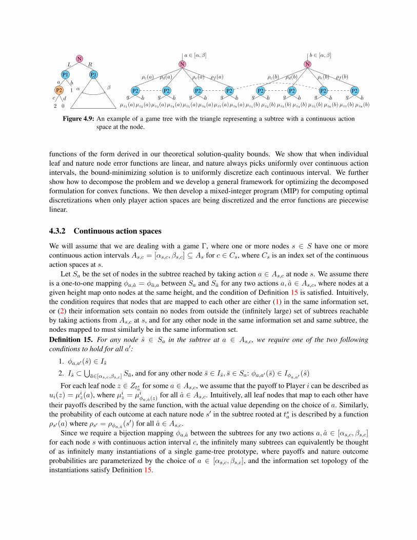
N

P1

P2

2

c

0

d

a

1

b

L

P1

R

βα

N

P2

µz1(a)

g

µz2(a)h

ρc(a)

P2

µz3(a)

g

µz4(a)h

ρd(a)

P2

µz5(a)

g

µz6(a)h

ρe(a)

P2

µz7(a)

g

µz8(a)h

ρf (a)

a ∈ [α, β]

N

P2

µz1(b)

g

µz2(b)h

ρc(b)

P2

µz3(b)

g

µz4(b)h

ρd(b)

P2

µz5(b)

g

µz6(b)h

ρe(b)

P2

µz7(b)

g

µz8(b)h

ρf (b)

b ∈ [α, β]

Figure 4.9: An example of a game tree with the triangle representing a subtree with a continuous actionspace at the node.

functions of the form derived in our theoretical solution-quality bounds. We show that when individualleaf and nature node error functions are linear, and nature always picks uniformly over continuous actionintervals, the bound-minimizing solution is to uniformly discretize each continuous interval. We furthershow how to decompose the problem and we develop a general framework for optimizing the decomposedformulation for convex functions. We then develop a mixed-integer program (MIP) for computing optimaldiscretizations when only player action spaces are being discretized and the error functions are piecewiselinear.

4.3.2 Continuous action spaces

We will assume that we are dealing with a game Γ, where one or more nodes s ∈ S have one or morecontinuous action intervals As,c = [αs,c, βs,c] ⊆ As for c ∈ Cs, where Cs is an index set of the continuousaction spaces at s.

Let Sa be the set of nodes in the subtree reached by taking action a ∈ As,c at node s. We assume thereis a one-to-one mapping φa,a = φa,a between Sa and Sa for any two actions a, a ∈ As,c, where nodes at agiven height map onto nodes at the same height, and the condition of Definition 15 is satisfied. Intuitively,the condition requires that nodes that are mapped to each other are either (1) in the same information set,or (2) their information sets contain no nodes from outside the (infinitely large) set of subtrees reachableby taking actions from As,c at s, and for any other node in the same information set and same subtree, thenodes mapped to must similarly be in the same information set.Definition 15. For any node s ∈ Sa in the subtree at a ∈ As,c, we require one of the two followingconditions to hold for all a′:

1. φa,a′(s) ∈ Is2. Is ⊂

⋃a∈[αs,c,βs,c]

Sa, and for any other node s ∈ Is, s ∈ Sa: φa,a′(s) ∈ Iφa,a′ (s)For each leaf node z ∈ Ztsa for some a ∈ As,c, we assume that the payoff to Player i can be described as

ui(z) = µiz(a), where µiz = µiφa,a(z) for all a ∈ As,c. Intuitively, all leaf nodes that map to each other havetheir payoffs described by the same function, with the actual value depending on the choice of a. Similarly,the probability of each outcome at each nature node s′ in the subtree rooted at tsa is described by a functionρs′(a) where ρs′ = ρφa,a(s′) for all a ∈ As,c.

Since we require a bijection mapping φa,a between the subtrees for any two actions a, a ∈ [αs,c, βs,c]for each node s with continuous action interval c, the infinitely many subtrees can equivalently be thoughtof as infinitely many instantiations of a single game-tree prototype, where payoffs and nature outcomeprobabilities are parameterized by the choice of a ∈ [αs,c, βs,c], and the information set topology of theinstantiations satisfy Definition 15.

An example game is shown in Figure 4.9. On the left is a game with three players: nature(N ), Player1 (P1), and Player 2 (P2). Nature first chooses between L and R (with some unspecified fixed probabilitydistribution). If L is chosen, a discrete subgame is reached. IfR is chosen, P1 has a continuous action space[α, β]. In the middle and right are shown two specific subtrees under the continuous action space, for P1choosing actions a, b ∈ [α, β], respectively. The information set that spans across the trees is an exampleof one that satisfies Condition 1 of Definition 15, while the one that does not span across the trees satisfiesCondition 2.

So far we have described our notation in terms of discretizing a single continuous action space at somenode. When there is more than one node with a continuous action space that is being discretized, we haveto consider two groups of nodes with continuous action spaces.

The first group is the set of all nodes s that have one or more continuous action intervals, and s is the firstnode on the path from the root to s with a continuous action space. Let the set of all such nodes be S1 ⊆ S.These nodes are handled exactly as described above. If there are additional continuous action spaces in thesubtree after taking some action a ∈ As,c for some s, c, then the bijections between subtrees simply mapuncountably many nodes.

The second group is the set of all nodes s′ such that there is at least one node-action pair s, a on the pathfrom the root to s′, where s has a continuous action space As,c such that a ∈ As,c. Let this set of nodes becalled S2 ⊂ S. Let ~a ∈ Rn, where n is the number of continuous action spaces leading to s′ and includingthe one at s′, such that ai ∈ [αi, βi] where [αi, βi] is the continuous action space for the i’th node with acontinuous action space on the path to s′. We then require that the payoff and nature functions are functionsof ~a rather than a single action choice. For fixed choices in the past, the functions then behave exactly as thefunctions for nodes in S1.

We fix some ordering of all continuous intervals, and define A = ×s∈S1∪S2,c∈CsAs,c to be the Cartesianproduct over all continuous intervals. We will use j to denote indices into this ordering I. We let [αj , βj ]denote the endpoints of interval j ∈ I. From now on we will use ~a ∈ A to denote elements of this set. Adiscretization is a finite set of points A′ ⊂ A. The size |A′| = m is the number of discrete points chosen foreach interval. If fewer than m points are desired for some interval As,c with index j ∈ I, we can simply let~aj = ~a′j for distinct points ~a,~a′ ∈ A′. For a node s, we will use ~as to refer to the subset of actions taken onthe path to s such that the action is part of a continuous action interval. We will overload the notation of thepayoff and nature error functions so that for a given f or h for a node s, they take elements ~a ∈ A as input,with the implicit understanding that the value of the function depends only on ~as. We will let π0(~a) denotethe product of probabilities over each index j into ~a such that nature acts at ~aj .

The game Γ′ = 〈N,A′, S′, Z ′,H, σ0, u, I ′〉 is the discrete extensive-form game obtained by restrictingplayers to selecting actions that are part of the discretization A′.

4.3.3 Discretization model

Discretization mapping and error terms

We will need to reason about the similarity of the full game Γ and the induced game Γ′ for a given dis-cretization A′. To do this we will require a mapping of the continuous action space onto the discretization:Definition 16. A discretization mapping is a surjective function g : A→ A′ that maps the continuous actionspace A onto the discretization A′. We require that g is decomposable, so for all ~a ∈ A, g(~a)j depends onlyon ~aj . GA′ denotes the set of legal discretization maps for a given discretization A′.

The discretization mapping along with the bijections φa,a′ for all s ∈ S, c ∈ Cs, a, a′ ∈ As,c immedi-ately defines a mapping of the nodes S onto the nodes S′. Denote this node mapping function by h : S → S′.

For any node s ∈ S∩S′, h(s) = s. For s ∈ S, s /∈ S′, h(s) is the node in S′ reached by inductively applyingthe maps g and φ~asj ,g(~as)j at each continuous action space on the path to s.

Due to the constraints in Definition 15, g also leads to an information set mapping, as any two nodess1, s2 ∈ I for some I must map to the same information set: h(s1), h(s2) ∈ I ′ for some I ′. We letf : I → I ′ be this information set mapping.

For all three functions g, h, f we also define their inverses g−1, h−1, f−1, that return all intervals A ⊆ A,nodes S ⊂ S, and information sets I ⊆ I, respectively, that map onto given ~a ∈ A′, s′ ∈ S′, and I ′ ∈ I ′,respectively. We denote by h−1

I (s′) the intersection h−1(s′) ∩ I .Given a discretization mapping g, it will be convenient to define aggregate utility error terms for nodes

of the real game:

εRs,i =

maxa∈As ε

Rtsa,i

if s is a player node∫a∈As σ0(s, a)εRtsa,i if s is a nature node∣∣µis(~a)− µis(g(~a))

∣∣ if s is a leaf node

Similarly, we define aggregate error terms for nature error. We define the nature distribution error of aninformation set I and node s′ ∈ f(I) to be

ε0I,s′ =

∣∣∣∣∣∫s∈h−1

I (s′) σ0(s)

σ0(I)− σ′0(s′)

σ′0(f(I))

∣∣∣∣∣This is the difference between nature’s probability of reaching s′ and its probability of reaching any nodein h−1

I (s′), normalized by the probability of reaching the given information sets. The nature error forinformation set I is

ε0I =∑

s′∈f(I)

ε0I,s′

For a nature node s at height k ∈ H0 and s′ = h(s), we define the nature action a′ ∈ As′ error and nodeerror to respectively be

ε0s,s′,a′ =

∣∣∣∣∣σ′0(s′, a′)−∫a∈g−1(a′)∩As

σ0(s, a)

∣∣∣∣∣ε0s =

∑a′∈As′

ε0s,s′,a′

The nature error at height k is

ε0k =

∫I∈Ik π(I)ε0I if k /∈ H0∫s∈Sk π(s)ε0s if k ∈ H0

Finally, we let W = maxi∈N,z∈Z ui(z) be the maximum payoff at any leaf node.

Strategy mapping

Once a Nash equilibrium has been computed in the discretized game, we need to define a way of convertingthat strategy profile to a strategy profile for the full game. We perform this mapping in the following simpleway. Since all subtrees under discretized intervals have the same shape (based on how we defined the

Nash equilibrium ε-Nash equilibrium

Discrete game

Discretization

Equilibrium-finding algorithm

Map to real game

Real game

Figure 4.10: An overview of our discretization approach.

discretization problem in Section 4.3.2) and thus same number of actions, we can simply implement thesame strategy that we computed for a given discretized subtree at all subtrees that map to it. Specifically,let σ′ be the strategy profile computed for the discretized game. Then for each real node s ∈ S, we setσ(s, a) = σ′(h(s), a′), where a′ is the action at s′ that leads to h(tsa). For continuous intervals, we simplypick each discrete point a with the probability that it was chosen in the discrete game, and every other actionwith probability zero. This mapping yields a strategy profile that satisfies the following property, which wewill use to derive bounds later:

Proposition 9. For a strategy profile σ′ computed in a discretized game Γ′, our method of strategy conver-sion leads to a strategy profile σ for the full game Γ so that for any information set pair I, I ′ such that Imaps onto I ′, σ−0(I) > 0, and σi(I) > 0,

∣∣∣∣∣∣∣σ(s′)

σ(I ′)−

∑s∈g−1

I (s′)

σ(s)

σ(I)

∣∣∣∣∣∣∣ ≤ ε0I,s′

4.3.4 Overview of our approach

Given some game with continuous action spaces, the goal in this work is to pick a finite set of points foreach continuous action interval. This will induce a finite extensive-form game. A (potentially approximate)Nash equilibrium is then computed in the discrete game. The computed Nash equilibrium is then mappedto a strategy profile in the full (continuous) game. Figure 4.10 illustrates the approach.

Under reasonable assumptions, we will derive solution quality bounds for any Nash equilibrium com-puted in the abstraction when implemented in the full game. More specifically, we will show that suchstrategy profiles constitute ε-Nash equilibria in the full game, where the ε depends on the error terms wedefined in the previous section. These results are anlogous to the solution-quality results for perfect-recallabstraction in Section 4.1.

4.3.5 Discretization quality bounds

We start by showing an error bound on solution quality for any given discretization and discretization map-ping, leveraging Theorem 7.Theorem 14. For any game Γ with continuous action spaces A that satisfy the constraint given in Defini-tion 15, discretization A′ ⊂ A, and discretization mapping g : A → A′, any Nash equilibrium σ computedin Γ′ constitutes an ε-Nash equilibrium when implemented in Γ, where

ε = maxi

2εRs,i +

∑k∈Hi

ε0kW

+ 2∑k∈H0

ε0kW

The bounds as given here are in their most general form. In particular, the two nature error terms∑k∈Hi ε

0kW and 2

∑k∈H0

ε0kW are not given in terms of the functions ρs that describe the change in natureoutcome probabilities. ε0k can easily be bounded for all k inHi andH0 respectively:

ε0k ≤∫I∈Ik

π(I)∑

s′∈f(I)

∣∣∣∣∣∫s∈h−1

I (s′)π0(~as)− π0(~as

′)

∣∣∣∣∣ = ξ0k

ε0k ≤∫s∈Sk

π(s)∑a′∈As′

∣∣∣∣∣∫a∈g−1

I (a′)σ0(s, a)− σ0(s′, a′)

∣∣∣∣∣ = ξ0k

This gives the following corollary:Corollary 1. For any game Γ with continuous action spaces A that satisfy the constraint given in Defini-tion 15, discretization A′ ⊂ A, and discretization mapping g : A → A′, any Nash equilibrium σ computedin Γ′ constitutes an ε-Nash equilibrium when implemented in Γ, where

ε = maxi

2εRs,i +

∑k∈Hi

ξ0kW

+ 2∑k∈H0

ξ0kW

The ξ0k terms do not diverge. While an infinite sum is taken in both cases, the terms are probability

weighted, and∫I∈Ik π(I) = 1,

∫s∈Sk π(s) = 1. Since we are dealing with probability distributions, we can

take the maximum over Ik or Sk. In practical settings, it may be desireable to take several maxima. First,in the current form of both Theorem 14 and Corollary 1, the bound depends on the strategy profile of theplayers, not just nature. To make the bound independent of player actions, one can take the maximum overplayer actions. Second, instead of computing the infinite sum of errors over Ik or Sk, it may be useful totake the probability-weighted sum of errors over discrete points, and then compute the maximum error overeach discrete point.

4.3.6 Discretization algorithms

In this section we consider general bounded discretization problems that are largely independent of thespecific error bound to be minimized. This means that our algorithms will apply to the results from Sec-tion 4.3.5, and also to any (potentially stronger or more general) bounds obtained in the future, as long asthey fall under the setting described in Section 4.3.6.

Optimal discretization as an optimization problem

We consider a more general class of problems than those described in Section 4.3.2. We consider a gameΓ where one or more s ∈ S has a continuous action space. We again let A be the set of all intervals to bediscretized with index set I and let ~alj refer to the kj discrete points chosen for interval j. We assume thepoints in the discretization are ordered, so ~alj < ~al+1

j for all j ∈ I, l ∈ [kj ].We start by formulating the optimization problem very generally. We assume that we have an error

bounding function Ψ : Ak × GA → R that takes as input a discretization A′ and discretization map g andreturns a real-valued error bound Ψ(A′, g). We make two innocuous assumptions about Ψ to represent thenatural condition that the error increases the further an actual point is from the discrete point to which itmaps.

First, each point maps to its nearest lower or upper discrete point. Formally, for all j ∈ I, and any pointal, ~alj < al < ~al+1

j not in the discretization, Ψ is minimized at g(al) = ~alj or g(al) = ~al+1j .

Second, for all j ∈ I, and any two points al, al, ~alj < al < al < ~al+1j not in the discretization, if

Ψ is minimized when g(al) = ~alj then Ψ is minimized when g(al) = ~alj , and if Ψ is minimized wheng(al) = ~al+1

j then Ψ is minimized when g(al) = ~al+1j .

We will say that an error function Ψ that satisfies our two assumptions is monotonic. Given a monotonicΨ and a discretization A′, the optimal mapping for each interval j ∈ I can be determined by finding thesplitting point between each interval

[~alj ,~a

l+1j

]such that the left side of the splitting point is mapped onto

~alj and right side is mapped onto ~al+1j .

For each interval j ∈ I, we introduce real-valued variables ~alj ∈ Aj , l ∈ [kj ] and gτs,c, τ ∈ [kj − 1],where kj is the desired number of discrete points for interval Aj . The variables ~alj represent the discretepoints, while gτj represents the point between ~aτj and ~aτ+1

j that separates the interval, such that the points in

the interval[~aτj , g

τj

]map onto ~aτj and the points in the interval

[gτj ,~a

τ+1j

]map onto ~aτ+1

j . Since any set of

values for ~alj , gτj over all j ∈ I, l ∈ [kj ] , τ ∈ [kj − 1] completely specifies a discretization and discretization

mapping, we let A′v, gv denote the discretization and mapping obtained by a solution. The feasible set ofthis problem is

F =

A′v, gv :

~alj ≤ ~al+1j ∀j ∈ I, l ∈ [kj − 1]

~aτj ≤ gτj ≤ ~aτ+1j ∀j ∈ I, τ ∈ [kj − 1]

~alj ∈ Aj ∀j ∈ I, l ∈ [kj ]

gτj ∈ Aj ∀j ∈ I, τ ∈ [kj − 1]

(4.13)

With this notation, we arrive at the most generic form of the optimal discretization problem for mono-tonic error functions:

min

Ψ(A′v, gv) :(A′v, gv

)∈ F

(4.14)

Setting k = 1, one can see that this is equivalent to minimizing any function, so this general form willnot get us far. Fortunately, there is often further structure in practical games. In the rest of the algorithmssection, we will consider various forms of structure that enable us to design efficient algorithms for findinggood discretizations.

Convex error function The constraints specified in (4.13) are all linear. Thus, if Ψ is convex, solving(4.14) becomes a convex minimization problem over linear constraints. These are solvable in polynomial

time under mild assumptions [Ben-Tal and Nemirovski, 2001]7. Perhaps more importantly, large subsets ofthis class of error functions have practically efficient solution methods—e.g., an error function that is conic-quadratic or semi-definite representable (Ben-Tal and Nemirovski [2001] give a thorough discussion of suchrepresentability), smooth, or non-smooth with certain structure [Nesterov, 2005b, Beck and Teboulle, 2012].

Decomposable error function

In Section 4.3.5, we considered error functions that are a mixture of maximums (player nodes) and probability-weighted sums (nature nodes) of the error functions at individual nodes. We now consider how to (recur-sively) represent such error functions using linear inequalities, for the purpose of computation.

Let ξj : Aj × gj → R be an error function that gives the error incurred at interval j ∈ I when choosingdiscretization A′j and mapping gj at Aj . Recursively taking the maximum or weighted sum can be imple-mented by recursively applying the following linear inequalities, where variable eδ represents the error at agiven node or information set δ:

E =

es ≥

∑a∈As

σ0(s, a)etsa

es ≥maxa∈As

etsa

es ≥ξj

(4.15)

The same linear formulation can also be used to formulate the error bound in the case where ξs : A× g arefunctions that give the error for each leaf and nature node. In a slight abuse of notation, we denote the set oferror function solutions described in (4.15) by E .

If each error function ξj depends only on the subset of A that consists of interval j and any descendantintervals, the discretization problem can be decomposed: find each interval j ∈ I that is the first continuousinterval from the root to the interval. Each such interval, along with its subtrees and any intervals therein,can be minimized separately.

Minimizing our bound

We will now study the game class that satisfies Definition 15 and minimization of the bound given in Corol-lary 1. We will consider various types of error functions.

Linear error functions In this section we consider games Γ where the utility and nature outcome dis-tribution functions µz, ρs, at all z ∈ Z, s ∈ S that are descendants of a continuous interval, are Lipschitzcontinuous with Lipschitz constant Lz/s. This encompasses two important practical classes of game: (1) allthe functions µ and ρ are linear, and (2) the functions are non-linear but the bound being derived is based onknowing (only) that the functions are Lipschitz continuous.

If all continuous intervals at nature nodes have a uniform distribution, we get the following simpleresults: all intervals should be discretized into uniform interval sizes.Theorem 15. For a game Γ with continuous action spaces A, where each utility and nature outcome dis-tribution function is Lipschitz continuous with constant Lz/s for each leaf z or nature node s, and allcontinuous nature intervals are uniformly distributed, the bound-minimizing kj-point discretization at each

7 A heavily updated version of this book is at http://www2.isye.gatech.edu/˜nemirovs/.

http://www2.isye.gatech.edu/~nemirovs/

interval A′j is:

~alj = αj +

(l − 1

2

)·(βj − αjkj

)∀l ∈ [kj ]

gτj = αj + τ ·(βj − αjkj

)∀τ ∈ [kj − 1]

We will call this a uniform discretization.When the conditions of the above theorem do not hold, the decomposition results from Section 4.3.6

and the recursive linearization (4.15) still apply. In the following two subsections, we leverage this fact.

Convex error functions As we pointed out above, taking the maximum, sum, and integral all preserveconvexity. Thus, if the error ∣∣µz(a)− µz(a′)

∣∣ or∣∣ρs(a)− ρ(a′)

∣∣at each leaf or nature node can be represented by a convex function, the linear constraints in (4.15) can beused to represent the overall error as a convex function. As discussed in Section 4.3.6, this would, dependingon the specific structure, allow the application of various efficient polynomial-time methods. We do not givespecific algorithms here, but merely point out that optimal solutions can be found in polynomial time. Inpractice, the specific choice of which polynomial-time algorithm to apply should be informed by the exactstructure of the error functions of the given game.

Piecewise linear error functions We now consider piecewise linear utility error functions and piecewiselinear nature probability error functions for discretizing continuous player action intervals. We do not con-sider discretizing nature actions here because even with linear functions and a uniform nature distribution,discretizing nature intervals would lead to quadratic error, as shown in the proof of Theorem 15. Even if theactual error functions are not piecewise linear, this can be used for arbitrarily accurate approximation.

Finding a bound-minimizing discretization, subject to a limit on the number of discretization points,is NP-hard. This is easily seen from Theorem 9, and representing their discrete game-abstraction problemusing a step function.

However, it can be represented by a MIP, where the number of binary variables is equal to the numberof pieces summed over all functions. This number can be significantly decreased if the interval pieces overthe different functions µ, ρ under some interval j ∈ I align. We use the same variable formulation ~alj , g

lj

as defined in (4.13), and the feasible set F remains the same. Consider an interval j ∈ I and the set ofpoints where some function in the subtrees at j changes piece. This set of points divides the interval [αj , βj ]into pieces. Let Pj be an index set into these pieces. The size of Pj is clearly bounded by the sum ofpieces in functions in subtrees at j. We introduce a Boolean variable bγ,lj , cγ,τj for each γ ∈ Pj , l ∈ [kj ],and τ ∈ [kj − 1], representing whether ~alj , g

τj fall into the interval representing piece γ ∈ Pj , respectively.

When bγ,lj (cγ,τj ) = 1, we restrict ~alj(gτj ) as follows:

αγj · bγ,lj ≤ ~a

lj , ~alj ≤ β

γj + (βj − βγj ) · bγ,lj

The sum∑

γ∈Pj bγ,lj = 1 ensures that only one interval is chosen. The constraints for cγ,τj , gτj are completely

analogous. For each leaf node z with piecewise payoff function µγz , and l ∈ [kj ], we can then introduce price

variables plz, plz(~a

lj), p

lz(g

lj) ∈ R, with the latter two for the interval

[~alj , g

lj

], and constrain them linearly as

follows:

P =

plz ≥plz(glj)− plz(~alj)

plz(glj) ≥µγz (glj)−M · c

γ,τj ∀γ ∈ Pj

plz(~alj) ≤µγz (~alj) +M · bγ,lj ∀γ ∈ Pj

(4.16)

This is correct for sufficiently large M ∈ R. We now have variables plz representing each error functionfor the discrete points, and can apply the linear constraints from (4.15) to get a linear representation of theoverall error. Thus we get the following MIP, where er is the objective value at the root according to (4.15):

miner : er ∈ E ,

(A′v, gv

)∈ F ∩ P, bγ,lj , cγ,τj ∈ 0, 1

(4.17)

4.3.7 Applications

In this section, we discuss some applications of our results. We will focus on three recent problems that haveincluded continuity in their problem formulation, or discretized away continuity: robust policy optimizationunder parameter uncertainty Chen and Bowling [2012], security games Yin and Tambe [2012], Kiekintveldet al. [2011], Marecki et al. [2012], and sequential wifi-jamming under battery constraints DeBruhl et al.[2014].

Chen and Bowling [2012] propose the use of zero-sum extensive-form game solving as a way of tractablycomputing optimally robust policies for Markov Decision Processes (MDPs) with parameter uncertainty.They design robustness criteria that can be implemented via nature first sampling parameter instances, andan opponent then choosing the worst of these. This sampling by nature was necessary in order to get gameswhere the action space for the players is finite. Now, with our discretization-quality results, it is possibleto use a broader class of robustness measures that allow continuous action spaces, while obtaining solutionquality bounds.

Several papers have investigated continuous settings for security games. These have been for single-shot Kiekintveld et al. [2011], Yin and Tambe [2012] or repeated Bayesian Stackelberg games Marecki et al.[2012]. Since our framework is for the more general setting of extensive-form games, our solution-qualitybounds apply to all these settings. Furthermore, they would also apply to more sophisticated models thatinclude both sequential actions and imperfect information. Marecki et al. [2012] mention as future work thesetting where the follower also behaves strategically. Our results immediately yield solution quality boundsfor discretizations for this setting.

Another area with continuity is wifi jamming. In recent work, sequential-interaction models were intro-duced for this domain DeBruhl et al. [2014]. These models employ discretized action spaces, where boththe jammer and transmitter have a (small) finite set of possible power levels to transmit at. However, this isan abstraction of reality, where software-defined radios mean that action spaces can be continuous (at leastup to the bit-precision of the hardware). Using the techniques developed in this paper, we can give solutionquality bounds on the utility loss obtained from considering only a discrete number of possible power levels(possibly by padding the game tree with dummy actions to satisfy Definition 15). DeBruhl et al. [2014] alsomention that in a more realistic model, both transmitter and jammer would be modeled as observing onlynoisy signals of the actions taken by the other player. Since these observations would be of a continuum,the noise would likewise be continuous. The discretization quality bounds derived here would immediatelyapply to this setting.

4.3.8 Differences to abstraction practice in poker

We have already discussed how our framework can be used to give theoretical bounds on solution quality inpractical scenarios. In particular, we showed that a uniform discretization is optimal for linear error functions(for discretizing nature this required a uniform distribution over the continuous action space). This standssomewhat in contrast to how practical abstractions are created for poker.

Consider no-limit Texas hold’em (NLHE). This game is the premier testbed for (discrete) extensive-form game solving algorithms [Sandholm, 2010]. Each year, the Annual Computer Poker Competition isheld, where research groups submit highly-tuned poker-playing programs. The winning programs are basedon computing Nash equilibrium approximations in abstractions of the full extensive-form game [Sandholm,2010].

In NLHE, at each betting step, the acting player may bet any amount from the minimum bet to their entirestack of chips. To handle this action space, the top agents devise betting abstractions. These are completelyanalogous to the discretizations considered in this paper. The payoff functions under the subtrees are alllinear in the specific actions chosen. At a cursory glance, one might say that Theorem 15 suggests thatthe optimal discretization would be uniform. However, the discretizations employed by the poker bots aremore akin to a geometric progression. For example, Brown et al. [2015] describe using a betting abstractionconsisting of 0.5, 0.75, 1, 1.5, 2 and 5 times the pot size, as well as the all-in action. At the start of betting,all-in is approximately 133 times the pot size. Both examples and experiments by Ganzfried and Sandholm[2013] support the idea that the uniform mapping is not optimal.

A potential explanation for this is that the subtrees reached for different choices of bet size technicallydo not fall under the constraints of Definition 15. Consider a group of bets, say raising in the range of [1, 2](here we consider continuous bets in this small continuous range due to ease of exposition, one can constructsimilar examples with larger integer ranges) with a stack size of 2.5. The subtree where the player bets 2exists as a subset of the subtree at every other betsize. These subsets all map to each other in a way thatobeys Definition 15. However, if the player bets 1 instead, the opponent may reraise by 1, in which case theagent can call. This scenario does not exist when betting 2, as the player already bet her entire stack. Forany two bet sizes a1 < a2, these discrepancies due to extra actions exist. To resolve this issue, one couldpad the tree with extra actions such that Definition 15 is satisfied, but it is unclear how this would interactwith the solution-quality bound, and could thus lead to nonoptimality of the uniform discretization.

4.3.9 Conclusions

We analyzed the problem of developing solution-quality bounds for discretization of extensive-form gameswith continuous action spaces. To our knowledge, we developed the first such bounds. We developed boundsfor a very general class of continuous games: ones where there is a finite set of prototype trees, such thatthe instantiation of a given prototype has its nature probability outcomes and utilities parameterized by thechoice on the continuous intervals. We developed bounds both where they depend on the specific Nashequilibrium (Theorem 14) and where they are independent of the Nash equilibrium chosen (Corollary 1).

We then considered the problem of computing bound-minimizing discretizations. First we developedvery general bound-minimization formulations that allow a broad class of error-bounding functions. Wediscussed how such functions can be minimized in polynomial time when they are convex. We then consid-ered the more specific problem of minimizing our bound developed for Corollary 1. For the case where allutility error and nature probability error functions are Lipschitz continuous (without additional structure),and nature chooses uniformly over each continuous interval, we showed that the bound-minimizing solutionis to discretize uniformly. For the case where the error functions at individual nodes can be represented

by convex functions, we showed how to generate a convex optimization formulation of the overall prob-lem. We also developed a MIP for piecewise linear error functions, which can also be used for arbitrarilyaccurate approximation. We also showed how the problem can be decomposed into separately optimizablecomponents.

Ganzfried and Sandholm [2013] dicuss randomized mappings, where each real point has a probabilitydistribution over which of its nearest discrete points it maps to. Their experiments strongly suggest that suchrandomization is desirable. Incorporating randomized mappings in our work could potentially lead to betterdiscretizations, almost certainly in practice, and potentially also in theory. We leave this as future research.

4.4 Proposed work

While the above lines of work have provided much-need theoretical foundations for the area of abstraction inEFGs, there is still a lot of work to do in order to bridge the gap to practical abstraction work. All algorithmsmentioned in the preceding section require either 1) solving an integer program whose size is on the order ofmagnitude of the game tree (this can be improved to just the signal tree for games of ordered signals) [Kroerand Sandholm, 2014], or 2) solving for abstractions level-by-level with prohibitively strong constraints onthe type of abstraction allowed [Kroer and Sandholm, 2016a].

The main issue facing our theoretical framework (as well as that of Lanctot et al. [2012]) is that when weconsider a pair of information sets I, I ′ for merging, we require some form of mapping between the nodesin the two information sets. In this mapping, we require that any pair of nodes s ∈ I, s′ ∈ I ′ that map toeach other have the same path of information set-action pairs, over all players for perfect recall (this is, atleast, the most obvious way to satisfy Definition 9), over the opponents in the past and over all players inthe future for imperfect recall (explicitly required by Definition 13).

An example from a small poker game can elucidate this. Consider a poker game with three cards: king,queen, and jack. For an information set representing us holding a king, there will be nodes representing ouropponent holding a queen or jack. Similarly if we are holding a queen, our opponent has to have a king orjack. If we want to merge our two information sets for king and queen, it is clear that the two jack nodescan map to each other. But if we want to satify the constraints in Definitions 9 and 13, the king and queennodes cannot map to each other immediately, as they are on different information set-action pair paths forour opponent. Instead, we are then required to also perform this abstraction for our opponent. In a biggergame, these constraints end up making the space of feasible abstractions very small.

We propose developing practical methods for computing abstractions, while retaining bounds on thesolution quality. We propose two different directions that could potentially achieve this:• By allowing additional worst-case assumptions about paths such as the ones described above. This

will allow a trade-off between 1) allowing more flexible abstraction that violates the prior constraints,and 2) deteriorating the solution quality bound, as these violations would lead to worse bounds. Thiswill greatly expand the set of feasible abstractions, thereby potentially making the computationalproblem easier. In the best-case scenario, this new framework will allow analysis of a general level-by-level abstraction algorithm. Either this will be achieved by analyzing existing level-by-level algo-rithms such as Ganzfried and Sandholm [2014] or by developing new algorithms that explicitly usethe bound quality as an objective.

• Making stronger assumptions about the game structure. This would be similar to the work on games ofordered signals [Gilpin and Sandholm, 2007b], but would require potentially slightly stronger assump-tions (Section 4.1.5 suggests that stronger assumptions will be necessary). One concrete direction isto exploit just the private signals of the game for abstraction, since private signals are easier to prove

bounds for.Depending on our success in developing such a scheme, we will attempt one or more of:• Compute the first strategy with a meaningful bound on regret in NLTHE. Ideally, this would be

achieved by first computing some abstraction with bounded solution quality, and then applying ascalable equilibrium-finding algorithm to the abstraction. Alternatively, we may focus on develop-ing methodologies for ex-post bounded regret computation by developing a hybrid best-response andabstraction approach.

• Show that existing practical abstraction algorithms compute solutions with bounds on solution quality.• If we are unable to develop a practical algorithm with bounds, we will also explore whether a solution-

quality impossibility result can be proven about the type of abstraction that is employed in practice.

Chapter 5

Limited lookahead in sequential games

5.1 Introduction

Limited lookahead has been a central topic in AI game playing for decades. To date, it has been studiedin single-agent settings and perfect-information games—specifically in well-known games such as chess,checkers, Go, etc., as well as in random game tree models [Korf, 1990, Pearl, 1981, 1983, Nau, 1983, Nauet al., 2010, Bouzy and Cazenave, 2001, Ramanujan et al., 2010, Ramanujan and Selman, 2011]. In thispaper, we initiate the game-theoretic study of limited lookahead in imperfect-information games. Suchgames are more broadly applicable to practical settings—for example auctions, negotiations, security, cy-bersecurity, and medical settings—than perfect-information games. Mirrokni et al. [2012] conducted agame-theoretic analysis of lookahead, but they consider only perfect-information games, and the results arefor four specific games rather than broad classes of games. Instead, we analyze the questions for imperfectinformation and general-sum extensive-form games.

As is typical in the literature on limited lookahead in perfect-information games, we derive our resultsfor a two-agent setting. One agent is a rational player (Player R) trying to optimally exploit a limited-lookahead player (Player L). Our results extend immediately to one rational player and more than onelimited-lookahead player, as long as the latter all break ties according to the same scheme (statically, favor-ably, or adversarially—as described later in the paper). This is because such a group of limited-lookaheadplayers can be treated as one from the perspective of our results.

The type of limited-lookahead player we introduce is analogous to that in the literature on perfect-information games. Specifically, we let the limited-lookahead player L have a node evaluation function hthat places numerical values on all nodes in the game tree. Given a strategy for the rational player, at eachinformation set at some depth i, Player L picks an action that maximizes the expected value of the evaluationfunction at depth i + k, assuming optimal play between those levels. Our study is the game-theoretic,imperfect-information generalization of lookahead questions studied in the literature and we believe thismakes it interesting in its own right. However, the model also has applications such as biological games,where the goal is to steer an evolution or adaptation process (which typically acts myopically with lookahead1) [Sandholm, 2015] and security games where opponents are often assumed to be myopic (as makes sensewhen the number of adversaries is large [Yin et al., 2012]). Furthermore, investigating how well a rationalplayer can exploit a limited-lookahead player lends insight into the limitations of using limited-lookaheadalgorithms in multiagent decision making.

We then design algorithms for finding an optimal strategy to commit to for the rational player. We focuson this rather than equilibrium computation because the latter seems nonsensical in this setting: the limited-

65

lookahead player determining a Nash equilibrium strategy would require her to reason about the whole gamefor the rational player’s strategy, which rings contrary to the limited-lookahead assumption. Computingoptimal strategies to commit to in standard rational settings has previously been studied in normal-formgames [Conitzer and Sandholm, 2006] and extensive-form games [Letchford and Conitzer, 2010], the latterimplying some complexity results for our setting as we will discuss.

As in the literature on lookahead in perfect-information games, a potential weakness of our approach isthat we require knowing the evaluation function h (but make no other assumptions about what informationh encodes). In practice, this function may not be known. As in the perfect-information setting, this can leadto the rational exploiter being exploited if their model of h is sufficiently wrong.

5.2 Model of limited lookahead

We now describe our model of limited lookahead. We use the term optimal hypothetical play to refer tothe way the limited-lookahead agent thinks she will play when looking ahead from a given information set.In actual play part way down that plan, she may change her mind because she will then be able to see to adeeper level of the game tree.

Let k be the lookahead of Player L, and SkI,a the nodes at lookahead depth k below information set I thatare reachable (through some path) by action a. As in prior work in the perfect-information game setting,Player L has a node-evaluation function h : S → R that assigns a heuristic numerical value to each node inthe game tree.

Given a strategy σR for the other player and fixed action probabilities for Nature, Player L chooses, atany given information set I ∈ IL at depth i, a (possibly mixed) strategy whose support is contained in theset of actions that maximize the expected value of the heuristic function at depth i + k, assuming optimalhypothetical play by her (maxσl in the formula below). We will denote this set by A∗I =

a : a ∈ arg maxa∈AI

maxσL

∑s∈I

πσ−L(s)

πσ−L(I)

∑s′∈SkI,a

πσ(tsa, s′)h(s′),

where σ = σL, σR is the strategy profile for the two players. Here moves by Nature are also countedtoward the depth of the lookahead. The model is flexible as to how the rational player chooses σR andhow the limited-lookahead player chooses a (possibly mixed) strategy with supports within the sets A∗I . Forone, we can have these choices be made for both players simultaneously according to the Nash equilibriumsolution concept. As another example, we can ask how the players should make those choices if one of theplayers gets to make, and commit to, all her choices before the other.

5.3 Complexity

In this section we analyze the complexity of finding strategies according to these solution concepts.

5.3.1 Nash equilibrium

Finding a Nash equilibrium when Player L either has information sets containing more than one node, orhas lookahead at least 2, is PPAD-hard [Papadimitriou, 1994]. This is because finding a Nash equilibriumin a 2-player general-sum normal-form game is PPAD-hard [Chen et al., 2009], and any such game can be

converted to a depth 2 extensive-form game (where the second player does not know what the first playermoved), where the general-sum payoffs are the evaluation function values.

If the limited-lookahead player only has singleton information sets and lookahead 1, an optimal strategycan be trivially computed in polynomial time in the size of the game tree for the limited-lookahead player(without even knowing the other player’s strategy σR) because for each of her information sets, we simplyhave to pick an action that has highest immediate heuristic value. To get a Nash equilibrium, what remainsto be done is to compute a best response for the rational player, which can also be easily done in polynomialtime [Johanson et al., 2011].

5.3.2 Commitment strategies

Next we study the complexity of finding commitment strategies. The complexity depends on whetherthe game has incomplete information (information sets that include more than one node) for the limited-lookahead player, how far that player can look ahead, and how she breaks ties in her action selection.

No information sets, lookahead 1, static tie-breaking As for the Nash equilibrium case, if the limited-lookahead player only has singleton information sets and lookahead 1, an optimal strategy can be triviallycomputed in polynomial time. We can use the same approach, except that the specific choice among theactions with highest immediate value is dictated by the tie-breaking rule. With this strategy in hand, findinga utility-maximizing strategy for Player R again consists of computing a best response.

No information sets, lookahead 1, adversarial tie-breaking When ties are broken adversarially, the choiceof response depends on the choice of strategy for the rational player. The set of optimal actions A∗s for anynode s ∈ SL can be precomputed, since Player R does not affect which actions are optimal. Player L willthen choose actions from these sets to minimize the utility of Player R. We can view the restriction to asubset of actions as a new game, where Player L is a rational player in a zero-sum game. An optimal strategyfor Player R to commit to is then a Nash equilibrium in this smaller game. This is solvable in polynomialtime by an LP that is linear in the size of the game tree [von Stengel, 1996], and algorithms have beendeveloped for scaling to large games [Hoda et al., 2010, Zinkevich et al., 2007, Lanctot et al., 2009, Kroerand Sandholm, 2014, 2016a, Gilpin and Sandholm, 2007b, Ganzfried and Sandholm, 2014].

No information sets, lookahead 1, favorable tie-breaking In this case, Player L picks the action from A∗sthat maximizes the utility of Player R. Perhaps surprisingly, computing the optimal solution in this case isharder than when facing an adversarial opponent.Theorem 16. Computing a utility-maximizing strategy for the rational player to commit to is NP-hard if thelimited-lookahead player breaks ties in favor of the rational player.

No information sets, lookahead > 1, favorable tie-breaking It is NP-hard to compute an optimal strategyto commit to in extensive-form games when both players are rational [Letchford and Conitzer, 2010]. Thatwas proven by reducing from knapsack to a 2-player perfect-information game of depth 4. This immediatelygives us two results: (1) finding an optimal strategy for Player R to commit to is NP-hard if Player L haslookahead at least 4, and (2) computing an optimal strategy to commit to for Player L is NP-hard even withlookahead 1. Their result also implies NP-hardness of computing a strategy to commit to for the rationalplayer, if our L player has lookahead of at least 4. We tighten this to lookahead 2:Theorem 17. Computing a utility-maximizing strategy for the rational player to commit to is NP-hard if thelimited lookahead player has lookahead at least 2.

Limited-lookahead player has information sets When the limited lookahead player has information sets,we show that computing a strategy to commit to is NP-hard:

Theorem 18. Computing a utility-maximizing strategy for the rational player to commit to is NP-hard if thelimited lookahead player has information sets of at least size 6.

5.4 Algorithms

In this section we will develop an algorithm for solving the hard commitment-strategy case. Naturally itsworst-case runtime is exponential. As mentioned in the introduction, we focus on commitment strategiesrather than Nash equilibria because Player L playing a Nash equilibrium strategy would require that playerto reason about the whole game for the opponent’s strategy. Further, optimal strategies to commit to aredesirable for applications such as biological games [Sandholm, 2015] (because evolution is respondingto what we are doing) and security games [Yin et al., 2012] (where the defender typically commits to astrategy).

Since the limited-lookahead player breaks ties adversarially, we wish to compute a strategy that max-imizes the worst-case best response by the limited-lookahead player. For argument’s sake, say that wewere given A, which is a fixed set of pairs, one for each information set I of the limited-lookaheadplayer, consisting of a set of optimal actions A∗I and one strategy for hypothetical play σIl at I . Formally,A =

⋃I∈Il〈A

∗I , σ

Il 〉. To make these actions optimal for Player L, Player R must choose a strategy such that

all actions in A are best responses according to the evaluation function of Player L. Formally, for all actiontriples a, a∗ ∈ A, a′ /∈ A (letting π(s) denote probabilities induced by σIL for the hypothetical play betweenI, a and s): ∑

s∈SkI,a

π(s) · h(s) >∑

s∈SkI,a′

π(s) · h(s) (5.1)

∑s∈SkI,a

π(s) · h(s) =∑

s∈SkI,a∗

π(s) · h(s) (5.2)

Player R chooses a worst-case utility-maximizing strategy that satisfies (5.1) and (5.2), and Player L hasto compute a (possibly mixed) strategy from A such that the utility of Player R is minimized. This can besolved by a linear program:Theorem 19. For some fixed choice of actions A, Nash equilibria of the induced game can be computed inpolynomial time by a linear program that has size O(|S|) +O(

∑I∈IL |AI | ·maxs∈S |As|k).

To prove this theorem, we first design a series of linear programs for computing best responses for thetwo players. We will then use duality to prove the theorem statement.

In the following, it will be convenient to change to matrix-vector notation, analogous to that of von Sten-gel [1996], with some extensions. Let A = −B be matrices describing the utility function for Player R andthe adversarial tie-breaking of Player L over A, respectively. Rows are indexed by Player R sequences, andcolumns by PlayerL sequences. For sequence form vectors x, y, the objectives to be maximized for the play-ers are then xAy, xBy, respectively. Matrices E,F are used to describe the sequence form constraints forPlayer R and L, respectively. Rows correspond to information sets, and columns correspond to sequences.Letting e, f be standard unit vectors of length |IR| , |IL|, respectively, the constraints Ex = e, Fy = fdescribe the sequence form constraint for the respective players. Given a strategy x for Player R satis-fying (5.1) and (5.2) for some A, the optimization problem for Player L becomes choosing a vector of y′

representing probabilities for all sequences inA that minimize the utility of PlayerR. Letting a prime super-script denote the restriction of each matrix and vector to sequences inA, this gives the following primal (5.3)and dual (5.4) LPs:

maxy′

(xTB′)y′

F ′y′ = f ′

y ≥ 0

(5.3)minq′

q′T f ′

q′TF ′ ≥ xTB′ (5.4)

where q′ is a vector with |A| + 1 dual variables. Given some strategy y′ for Player L, Player R maximizesutility among strategies that induce A. This gives the following best-response LP for Player R:

maxx

xT (Ay′)

xTET = eT

x ≥ 0

xTH¬A − xTHA ≤ −εxTGA∗ = xTGA

(5.5)

where the last two constraints encode (5.1) and (5.2), respectively. The dual problem uses the unconstrainedvectors p, v and constrained vector u and looks as follows

minp,u,v

eT p− ε · u

ET p+ (H¬A −HA)u+ (GA∗ −GA)v ≥ A′y′

u ≥ 0

(5.6)

We can now merge the dual (5.4) with the constraints from the primal (5.5) to compute a minimax strategy:Player R chooses x, which she will choose to minimize the objective of (5.4),

minx,q′

q′T f ′

q′TF ′ − xTB′ ≥ 0

−xTET = −eT

x ≥ 0

xTHA − xTH¬A ≥ εxTGA − xTGA∗ = 0

(5.7)

Taking the dual of this gives

maxy′,p

−eT p+ ε · u

−ET p+ (HA −H¬A)u+ (GA −GA∗)v ≤ B′y′

F ′y′ = f ′

y, u ≥ 0

(5.8)

The theorem follows by a duality proof on (5.7) and (5.8).In reality we are not given A. To find a commitment strategy for Player R, we could loop through

all possible structures A, solve LP (5.7) for each one, and select the one that gives the highest value. Wenow introduce a mixed-integer program (MIP) that picks the optimal induced game A while avoiding enu-meration. The MIP is given in (5.9). We introduce Boolean sequence-form variables that denote making

sequences suboptimal choices. These variables are then used to deactivate subsets of constraints, so that theMIP branches on formulations of LP (5.7), i.e., what goes into the structureA. The size of the MIP is of thesame order as that of LP (5.7).

minx,q,z

qT f

qTF ≥ xTB − zMEx = e

xTHA ≥ xTH¬A + ε− (1− z)MxTGA = xTGA∗ ± (1− z)M∑a∈AI

za ≥ za′

x ≥ 0, z ∈ 0, 1

(5.9)

The variable vector x contains the sequence form variables for Player R. The vector q is the set of dualvariables for Player L. z is a vector of Boolean variables, one for each Player L sequence. Setting za = 1denotes making the sequence a an inoptimal choice. The matrix M is a diagonal matrix with sufficientlylarge constants (e.g. the smallest value in B) such that setting za = 1 deactivates the corresponding con-straint. Similar to the favorable-lookahead case, we introduce sequence form constraints

∑a∈AI za ≥ za′

where a′ is the parent sequence, to ensure that at least one action is picked when the parent sequence isactive. We must also ensure that the incentivization constraints are only active for actions in A:

xTHA − xTH¬A ≥ ε− (1− z)M (5.10)

xTGA − xTGA∗ = 0± (1− z)M

for diagonal matrices M with sufficiently large entries. Equality is implemented with a pair of inequalityconstraints ≤,≥, where ± denotes adding or subtracting, respectively.

The values of each column constraint in (5.10) is implemented by a series of constraints. We add Booleanvariables σIL(I ′, a′) for each information set action pair I ′, a′ that is potentially chosen in hypothetical playat I . Using our regular notation, for each a, a′ where a is the action to be made dominant, the constraint isimplemented by: ∑

s∈SkI,a

vi(s) ≥ vdI (I), vi(s) ≤ σIL(I ′, a′) ·M (5.11)

where the latter ensures that vi(s) is only non-zero if chosen in hypothetical play. We further need theconstraint vi(s) ≤ πσ−L(s)h(s) to ensure that vi(s), for a node s at the lookahead depth, is at most theheuristic value weighted by the probability of reaching s.

5.5 Experiments

In this section we experimentally investigate how much utility can be gained by optimally exploiting alimited-lookahead player. We conduct experiments on Kuhn poker [Kuhn, 1950], a canonical testbed forgame-theoretic algorithms, and a larger simplified poker game that we call KJ. Kuhn poker consists of athree-card deck: king, queen, and jack. Each player antes 1. Each player is then dealt one of the three cards,and the third is put aside unseen. A single round of betting (p = 1) then occurs. In KJ, the deck consists of

two kings and two jacks. Each player antes 1. A private card is dealt to each, followed by a betting round(p = 2), then a public card is dealt, follower by another betting round (p = 4). If no player has folded, ashowdown occurs. For both games, each round of betting looks as follows:• Player 1 can check or bet p.

If Player 1 checks Player 2 can check or raise p.− If Player 2 checks the betting round ends.− If Player 2 raises Player 1 can fold or call.· If Player 1 folds Player 2 takes the pot.· If Player 1 calls the betting round ends.

If Player 1 raises Player 2 can fold or call.− If Player 2 folds Player 1 takes the pot.− If Player 2 calls the betting round ends.

In Kuhn poker, the player with the higher card wins in a showdown. In KJ, showdowns have two possibleoutcomes: one player has a pair, or both players have the same private card. For the former, the playerwith the pair wins the pot. For the latter the pot is split. Kuhn poker has 55 nodes in the game tree and 13sequences per player. The KJ game tree has 199 nodes, and 57 sequences per player.

To investigate the value that can be derived from exploiting a limited-lookahead opponent, a node eval-uation heuristic is needed. In this work we consider heuristics derived from a Nash equilibrium. For a givennode, the heuristic value of the node is simply the expected value of the node in (some chosen) equilibrium.This is arguably a conservative class of heuristics, as a limited-lookahead opponent would not be expectedto know the value of the nodes in equilibrium. Even with this form of evaluation heuristic it is possible toexploit the limited-lookahead player, as we will show. We will also consider Gaussian noise being addedto the node evaluation heuristic, more realistically modeling opponents who have vague ideas of the valuesof nodes in the game. Formally, let σ be an equilibrium, and i the limited-lookahead player. The heuristicvalue h(s) of a node s is:

h(s) =

ui(s) if s ∈ Z∑

a∈As σ(s, a)h(tsa) otherwise(5.12)

We consider two different noise models. The first adds Gaussian noise with mean 0 and standard deviationγ independently to each node evaluation, including leaf nodes. Letting µs be a noise term drawn fromN (0, γ): h(s) = h(s) + µs. The second, more realistic, model adds error cumulatively, with no error onleaf nodes:

h(s) =

ui(s) if s ∈ Z[∑

a∈As σ(s, a)h(tsa)]

+ µs otherwise(5.13)

Using MIP (5.9), we computed optimal strategies for the rational player in Kuhn poker and KJ. The MIPmodels were solved by CPLEX version 12.5. The results are given in Figure 5.1. The x-axis is the noiseparameter γ for h and h. The y-axis is the corresponding utility for the rational player, averaged over at least1000 runs per tuple 〈game, choice of rational player, lookahead, standard deviation〉. Each figure containsplots for the limited-lookahead player having lookahead 1 or 2, and a baseline for the value of the game inequilibrium without limited lookahead.

Figures 5.1a and b show the results for using evaluation function h in Kuhn poker, with the rationalplayer in plot a and b being Player 1 and 2, respectively. For rational Player 1, we see that, even with nonoise in the heuristic (i.e., the limited-lookahead player knows the value of each node in equilibrium), it is

0 0.2 0.4 0.6 0.8 1−0.1

−0.05

0

0.05

0.1

0.15

0.2

0.25

0.3

0.35

0.4

Standard deviation

Utilit

y

Lookahead 1

Lookahead 2

Value of game

(a) Kuhn Player 1, h

0 0.2 0.4 0.6 0.8 10.05

0.1

0.15

0.2

0.25

0.3

0.35

0.4

0.45

0.5

Standard deviation

Utilit

y

Lookahead 1

Lookahead 2

Value of game

(b) Kuhn Player 2, h

0 0.2 0.4 0.6 0.8 1

0

0.2

0.4

0.6

0.8

1

1.2

Standard deviation

Utilit

y

Lookahead 1

Lookahead 2

Value of game

(c) KJ Player 1, h

0 0.2 0.4 0.6 0.8 1−0.1

0

0.1

0.2

0.3

0.4

0.5

0.6

Standard deviation

Utilit

y

Lookahead 1

Lookahead 2

Value of game

(d) KJ Player 2, h

Figure 5.1: Winnings in Kuhn poker and KJ for the rational player as Player 1 and 2, respectively, forvarying per-node independent evaluation function noise. Error bars show standard deviation.

possible to exploit the limited-lookahead player if she has lookahead 1. (With lookahead 2 she achieves thevalue of the game.) For both amounts of lookahead, the exploitation potential steadily increases as noise isadded.

Figures 5.1c and d show the same variants for KJ. Here, lookahead 2 is worse for the limited-lookaheadplayer than lookahead 1. To our knowledge, this is the first known imperfect-information lookahead pathol-ogy. Such pathologies are well known in perfect-information games [Beal, 1980, Pearl, 1981, Nau, 1983],and understanding them remains an active area of research [Lustrek et al., 2006, Nau et al., 2010, Wilsonet al., 2012]. This version of the node heuristic does not have increasing visibility: node evaluations do notget more accurate toward the end of the game. Our experiments on KJ with h in Figures 5.2 g and h do nothave this pathology, and h does have increasing visibility.

Figure 5.3 shows a simple subtree (that could be attached to any game tree) where deeper lookaheadcan make the agent’s decision arbitrarily bad, even when the node evaluation function is the exact expected

(a) Kuhn Player 1, h

0 0.2 0.4 0.6 0.8 10.05

0.1

0.15

0.2

0.25

0.3

0.35

0.4

0.45

0.5

Standard deviation

Utilit

y

Lookahead 1

Lookahead 2

Value of game

(b) Kuhn Player 2, h

0 0.2 0.4 0.6 0.8 1

0

0.2

0.4

0.6

0.8

1

1.2

Standard deviation

Utilit

y

Lookahead 1

Lookahead 2

Value of game

(c) KJ Player 1, h

0 0.2 0.4 0.6 0.8 1

0

0.2

0.4

0.6

0.8

1

Standard deviation

Utilit

y

Lookahead 1

Lookahead 2

Value of game

(d) KJ Player 2, h

Figure 5.2: Winnings in Kuhn poker and KJ for the rational player as Player 1 and 2, respectively, forvarying cumulative evaluation function noise. Error bars show standard deviation.

value of a node in equilibrium.

P1 P2∗

P1∗

α

−α1

0

01

0

0

Figure 5.3: A subtree that exhibits lookahead pathology.

We now go over the example of Figure 5.3. Assume without loss of generality that all payoffs are positivein some game. We can then insert the subtree in Figure 5.3 as a subgame at any node belonging to P1, andit will be played with probability 0 in equilibrium, since it has expected value 0. Due to this, all strategieswhere Player 2 chooses up can be part of an equilibrium. Assuming that P2 is the limited-lookahead player

and minimizing, for large enough α, the node labeled P1∗ will be more desirable than any other node in thegame, since it has expected value −α according to the evaluation function. A rational player P1 can use thisto get P2 to go down at P2∗, and then switch to the action that leads to α. This example is for lookahead 1,but we can generalize the example to work with any finite lookahead depth: the node P1∗ can be replacedby a subtree where every other leaf has payoff 2α, in which case P2 would be forced to go to the leaf withpayoff α once down has been chosen at P2∗.

Figures 5.2e and f show the results for Kuhn poker with h. These are very similar to the results for h,with almost identical expected utility for all scenarios. Figures 5.1g and h, as previously mentioned, showthe results with h on KJ. Here we see no abstraction pathologies, and for the setting where Player 2 is therational player we see the most pronounced difference in exploitability based on lookahead.

5.6 Conclusions and future work

This chapter initiated the study of limited lookahead in imperfect-information games. We characterized thecomplexity of finding a Nash equilibrium and optimal strategy to commit to for either player. Figure 5.4summarizes those results, including the cases of favorable and static tie-breaking, the discussion of whichwe deferred to the extended online paper.

Information sets

PPAD,NP-hardLookahead depth > 1

Solution concept

Tie-breaking rule

NP-hardP

Adversarial, static FavorableP

Equilibrium CommitmentPPAD,NP-hard

yes no

no yes

Figure 5.4: Our complexity results. PPAD,NP-hard indicates that finding a Nash equilibrium (optimalstrategy to commit to) is PPAD-hard (NP-hard). P indicates polytime.

We then designed a MIP for computing optimal strategies to commit to for the rational player. Theproblem was shown to reduce to choosing the best among a set of two-player zero-sum games (the tie-breaking being the opponent), where the optimal strategy for any such game can be computed with an LP.We then introduced a MIP that finds the optimal solution by branching on these games.

We experimentally studied the impact of limited lookahead in two poker games. We demonstratedthat it is possible to achieve large utility gains by exploiting a limited-lookahead opponent. As one wouldexpect, the limited-lookahead player often obtains the value of the game if her heuristic node evaluation isexact (i.e., it gives the expected values of nodes in the game tree for some equilibrium)—but we provideda counterexample that shows that this is not sufficient in general. Finally, we studied the impact of noisein those estimates, and different lookahead depths. While lookahead 2 usually outperformed lookahead 1,we uncovered an imperfect-information game lookahead pathology: deeper lookahead can hurt the limited-lookahead player. We demonstrated how this can occur with any finite depth of lookahead, even if thelimited-lookahead player’s node evaluation heuristic returns exact values from an equilibrium.

Our algorithms in the NP-hard adversarial tie-breaking setting scaled to games with hundreds of nodes.For some practical settings more scalability will be needed. There are at least two exciting future directionstoward achieving this. One is to design faster algorithms. The other is designing abstraction techniquesfor the limited-lookahead setting. As noted in Chapter 4, abstraction plays an important role in large-scale

game solving [Sandholm, 2010]. Limited-lookahead games have much stronger structure, especially lo-cally around an information set, and it may be possible to utilize that to develop abstraction techniqueswith significantly stronger solution quality bounds. Also, leading practical game abstraction algorithms(e.g., [Ganzfried and Sandholm, 2014]), while theoretically unbounded, could immediately be used to in-vestigate exploitation potential in larger games. Finally, uncertainty over h is an important future researchdirection. This would lead to more robust solution concepts, thereby alleviating the pitfalls involved withusing an imperfect estimate.

5.7 Proposed work

The work developed in this chapter represents the first generalization of extensive-form game limited-lookahead research to the game-theoretic and imperfect-information setting. However, in order to be broadlyapplicable in practice, it is necessary to model uncertainty about the limited-lookahed behavior of the op-ponents. We propose extending the model developed in this chapter to include uncertainty over the node-evaluation function of the limited-lookahead player.

We will consider two types of uncertainty: uncertainty over a base set of functions hi : S → Rsampled before the game begins, or a stochastic node-evaluation function h : S → Xs, whereXs is an inde-pendent random variable representing the evaluation function at node s. The former is more likely to yieldresults; for example, we can model the uncertainty over the node-evaluation function as an initial chance-node appended to the game. The latter would lead to greater flexibility in modeling, and it could ideally becombined with the former. The latter, more general framework may be computationally difficult to handleif the goal is to maximize expected value. Expected value maximization has the drawback that it requires adistribution, and is therefore still unrealistic for some practical settings. Instead, we will investigate the useof robust optimization frameworks, which require fewer assumptions about the node-evaluation function,and are more likely to be practically computable. In particular, rather than try to maximize the expectedpayoff against some distributional assumption about the node-evaluation function, we will focus on show-ing robustness against any node-evaluation function from some uncertainty set. This will likely allow us toleverage algorithms for either robust convex or robust combinatorial optimization [Ben-Tal and Nemirovski,2002, Ben-Tal et al., 2009, Mutapcic and Boyd, 2009, Bertsimas et al., 2011]

Chapter 6

Timeline

My proposed research will roughly be completed as follows:January 2017: Proposal

January–February 2017: Large-scale equilibrium refinements (Section 3), submit to IJCAI

January–April 2017: Speeding up FOMs to be competitive with CFR at earlier stages of convergence(Section 3), submit first results to EC

May–July 2017: Show efficient implementation of FOMs on large games (Section 3)

June–August 2017: Robust optimization for uncertainty in limited lookahead (Section 5)

June–December 2017: Practical abstraction algorithms with solution-quality bounds (Section 4)

January–March 2018: Academic job interviews

March–April 2018: Writing my thesis document

May 2018: Thesis defense

76

Chapter 7

A brief overview of my non-thesis research

This chapter briefly surveys some of the research directions I have followed during my Ph.D. that are notincluded in my proposed thesis.• Prediction markets. In my work on prediction markets [Kroer et al., 2016], we present a new com-

binatorial market maker that operates arbitrage-free combinatorial prediction markets specified byinteger programs. Although the problem of arbitrage-free pricing, while maintaining a bound onthe subsidy provided by the market maker, is #P-hard in the worst case, we posit that the typicalcase might be amenable to modern integer programming (IP) solvers. At the crux of our method isthe Frank-Wolfe (conditional gradient) algorithm which is used to implement a Bregman projectionaligned with the market maker’s cost function, using an IP solver as an oracle. We demonstrate thetractability and improved accuracy of our approach on real-world prediction market data from combi-natorial bets placed on the 2010 NCAA Men’s Division I Basketball Tournament, where the outcomespace is of size 263. To our knowledge, this is the first implementation and empirical evaluation of anarbitrage-free combinatorial prediction market on this scale.

• Sequential planning for biological problems. In Kroer and Sandholm [2016b] we study biologicaladaptation, a powerful mechanism that makes many disorders hard to combat. We study steering suchadaptation through sequential planning. We propose a general approach where we leverage MonteCarlo tree search to compute a treatment plan, and the biological entity is modeled by a black-boxsimulator that the planner calls during planning. We show that the framework can be used to steera biological entity modeled via a complex signaling pathway network that has numerous feedbackloops that operate at different rates and have hard-to-understand aggregate behavior.

• Computational bundling. In Kroer and Sandholm [2015a], we study a common revenue-enhancementapproach—bundling—in the context of the most commonly studied combinatorial auction mecha-nism, the Vickrey-Clarke-Groves (VCG) mechanism. A challenge in mechanism design for combi-natorial auctions is that the prior distribution on each bidder’s valuation can be doubly exponential.Such priors do not exist in most applications. Rather, in many applications (such as premium displayadvertising markets), there is essentially a point prior, which may not be accurate. We adopt the pointprior model, and prove robustness to inaccuracy in the prior. Then, we present a branch-and-boundframework for finding the optimal bundling. We introduce several techniques for branching, upperbounding, lower bounding, and lazy bounding. Experiments on CATS distributions validate the ap-proach and show that our techniques dramatically improve scalability over a leading general-purposeMIP solver.

77

Bibliography

ACPC. Annual Computer Poker Competition website. http://www.computerpokercompetition.org/, 2016. [Online; accessed 23-Feb-2016].

C. Archibald and Y. Shoham. Modeling billiards games. In International Conference on Autonomous Agentsand Multi-Agent Systems (AAMAS), Budapest, Hungary, 2009.

Nicola Basilico and Nicola Gatti. Automated abstractions for patrolling security games. In AAAI Conferenceon Artificial Intelligence (AAAI), 2011.

Donald F Beal. An analysis of minimax. Advances in computer chess, 2:103–109, 1980.

Amir Beck and Marc Teboulle. Smoothing and first order methods: A unified framework. SIAM Journal onOptimization, 22(2):557–580, 2012.

Aharon Ben-Tal and Arkadi Nemirovski. Robust optimization–methodology and applications. MathematicalProgramming, 92(3):453–480, 2002.

Aharon Ben-Tal, Laurent El Ghaoui, and Arkadi Nemirovski. Robust optimization. Princeton UniversityPress, 2009.

Ahron Ben-Tal and Arkadi Nemirovski. Lectures on modern convex optimization: analysis, algorithms, andengineering applications, volume 2. Siam, 2001.

Dimitris Bertsimas, David B Brown, and Constantine Caramanis. Theory and applications of robust opti-mization. SIAM review, 53(3):464–501, 2011.

Darse Billings, Neil Burch, Aaron Davidson, Robert Holte, Jonathan Schaeffer, Terence Schauenberg, andDuane Szafron. Approximating game-theoretic optimal strategies for full-scale poker. In Proceedings ofthe 18th International Joint Conference on Artificial Intelligence (IJCAI), 2003.

Kellog S Booth and Charles J Colbourn. Problems polynomially equivalent to graph isomorphism. Com-puter Science Department, Univ., 1979.

B Bosansky, Christopher Kiekintveld, V Lisy, and Michal Pechoucek. An exact double-oracle algorithm forzero-sum extensive-form games with imperfect information. Journal of Artificial Intelligence Research,pages 829–866, 2014.

Bruno Bouzy and Tristan Cazenave. Computer go: an ai oriented survey. Artificial Intelligence, 132(1):39–103, 2001.

Michael Bowling, Neil Burch, Michael Johanson, and Oskari Tammelin. Heads-up limit hold’em poker issolved. Science, 347(6218):145–149, January 2015.

Noam Brown and Tuomas Sandholm. Regret transfer and parameter optimization. In AAAI Conference onArtificial Intelligence (AAAI), 2014.

78

http://www.computerpokercompetition.org/

http://www.computerpokercompetition.org/

Noam Brown and Tuomas Sandholm. Simultaneous abstraction and equilibrium finding in games. InProceedings of the International Joint Conference on Artificial Intelligence (IJCAI), 2015.

Noam Brown, Sam Ganzfried, and Tuomas Sandholm. Hierarchical abstraction, distributed equilibriumcomputation, and post-processing, with application to a champion no-limit Texas Hold’em agent. InInternational Conference on Autonomous Agents and Multi-Agent Systems (AAMAS), 2015.

Neil Burch, Marc Lanctot, Duane Szafron, and Richard G Gibson. Efficient monte carlo counterfactualregret minimization in games with many player actions. In Advances in Neural Information ProcessingSystems, pages 1880–1888, 2012.

Katherine Chen and Michael Bowling. Tractable objectives for robust policy optimization. In Proceedingsof the Annual Conference on Neural Information Processing Systems (NIPS), 2012.

Xi Chen, Xiaotie Deng, and Shang-Hua Teng. Settling the complexity of computing two-player Nashequilibria. Journal of the ACM, 2009.

Vincent Conitzer and Tuomas Sandholm. Computing the optimal strategy to commit to. In Proceedings ofthe ACM Conference on Electronic Commerce (ACM-EC), Ann Arbor, MI, 2006.

Constantinos Daskalakis, Alan Deckelbaum, and Anthony Kim. Near-optimal no-regret algorithms for zero-sum games. Games and Economic Behavior, 92:327–348, 2015.

Bruce DeBruhl, Christian Kroer, Anupam Datta, Tuomas Sandholm, and Patrick Tague. Power nappingwith loud neighbors: optimal energy-constrained jamming and anti-jamming. In Proceedings of the 2014ACM conference on Security and privacy in wireless & mobile networks, pages 117–128. ACM, 2014.

Gabriele Farina and Nicola Gatti. Extensive-form perfect equilibrium computation in two-player games. InAAAI Conference on Artificial Intelligence (AAAI), 2017.

Tomas Feder and Daniel Greene. Optimal algorithms for approximate clustering. In Proceedings of theAnnual Symposium on Theory of Computing (STOC), 1988.

Joaquim Gabarro, Alina Garcıa, and Maria Serna. On the complexity of game isomorphism. In Mathemati-cal Foundations of Computer Science 2007, pages 559–571. Springer, 2007.

Sam Ganzfried and Tuomas Sandholm. Tartanian5: A heads-up no-limit Texas Hold’em poker-playingprogram. In Computer Poker Symposium at the National Conference on Artificial Intelligence (AAAI),2012.

Sam Ganzfried and Tuomas Sandholm. Action translation in extensive-form games with large action spaces:Axioms, paradoxes, and the pseudo-harmonic mapping. In Proceedings of the International Joint Con-ference on Artificial Intelligence (IJCAI), 2013.

Sam Ganzfried and Tuomas Sandholm. Potential-aware imperfect-recall abstraction with earth mover’sdistance in imperfect-information games. In AAAI Conference on Artificial Intelligence (AAAI), 2014.

Richard Gibson, Marc Lanctot, Neil Burch, Duane Szafron, and Michael Bowling. Generalized samplingand variance in counterfactual regret minimization. In AAAI Conference on Artificial Intelligence (AAAI),2012.

Andrew Gilpin and Tuomas Sandholm. A competitive Texas Hold’em poker player via automated abstrac-tion and real-time equilibrium computation. In Proceedings of the National Conference on ArtificialIntelligence (AAAI), pages 1007–1013, 2006.

Andrew Gilpin and Tuomas Sandholm. Better automated abstraction techniques for imperfect informationgames, with application to Texas Hold’em poker. In International Conference on Autonomous Agents

and Multi-Agent Systems (AAMAS), pages 1168–1175, 2007a.

Andrew Gilpin and Tuomas Sandholm. Lossless abstraction of imperfect information games. Journal of theACM, 54(5), 2007b.

Andrew Gilpin and Tuomas Sandholm. Lossless abstraction of imperfect information games. Journal of theACM, 54(5), 2007c. Early version ‘Finding equilibria in large sequential games of imperfect information’appeared in the Proceedings of the ACM Conference on Electronic Commerce (EC), pages 160–169,2006.

Andrew Gilpin and Tuomas Sandholm. Expectation-based versus potential-aware automated abstractionin imperfect information games: An experimental comparison using poker. In Proceedings of the AAAIConference on Artificial Intelligence (AAAI), 2008. Short paper.

Andrew Gilpin, Tuomas Sandholm, and Troels Bjerre Sørensen. Potential-aware automated abstraction ofsequential games, and holistic equilibrium analysis of Texas Hold’em poker. In Proceedings of the AAAIConference on Artificial Intelligence (AAAI), 2007.

Andrew Gilpin, Tuomas Sandholm, and Troels Bjerre Sørensen. A heads-up no-limit Texas Hold’em pokerplayer: Discretized betting models and automatically generated equilibrium-finding programs. In Inter-national Conference on Autonomous Agents and Multi-Agent Systems (AAMAS), 2008.

Andrew Gilpin, Javier Pena, and Tuomas Sandholm. First-order algorithm with O(ln(1/ε)) convergencefor ε-equilibrium in two-person zero-sum games. Mathematical Programming, 133(1–2):279–298, 2012.Conference version appeared in AAAI-08.

Teofilo F Gonzalez. Clustering to minimize the maximum intercluster distance. Theoretical ComputerScience, 38, 1985.

Anupam Gupta, Guru Guruganesh, and Melanie Schmidt. Approximation algorithms for aversion k-clustering via local k-median. In 43rd International Colloquium on Automata, Languages, and Pro-gramming, ICALP, pages 66:1–66:13, 2016.

Joseph Y Halpern and Rafael Pass. Sequential equilibrium in computational games. In Proceedings of theTwenty-Third international joint conference on Artificial Intelligence, pages 171–176. AAAI Press, 2013.

John Hawkin, Robert Holte, and Duane Szafron. Automated action abstraction of imperfect informationextensive-form games. In AAAI Conference on Artificial Intelligence (AAAI), 2011.

John Hawkin, Robert Holte, and Duane Szafron. Using sliding windows to generate action abstractions inextensive-form games. In AAAI Conference on Artificial Intelligence (AAAI), 2012.

Jean-Baptiste Hiriart-Urruty and Claude Lemarechal. Fundamentals of convex analysis. 2001.

Samid Hoda, Andrew Gilpin, Javier Pena, and Tuomas Sandholm. Smoothing techniques for computingNash equilibria of sequential games. Mathematics of Operations Research, 35(2):494–512, 2010. Con-ference version appeared in WINE-07.

Albert Jiang and Kevin Leyton-Brown. Polynomial-time computation of exact correlated equilibrium incompact games. In Proceedings of the ACM Conference on Electronic Commerce (EC), 2011.

Michael Johanson, Kevin Waugh, Michael Bowling, and Martin Zinkevich. Accelerating best responsecalculation in large extensive games. In Proceedings of the International Joint Conference on ArtificialIntelligence (IJCAI), 2011.

Michael Johanson, Nolan Bard, Neil Burch, and Michael Bowling. Finding optimal abstract strategies inextensive-form games. In AAAI Conference on Artificial Intelligence (AAAI), 2012.

Michael Johanson, Neil Burch, Richard Valenzano, and Michael Bowling. Evaluating state-space abstrac-tions in extensive-form games. In International Conference on Autonomous Agents and Multi-AgentSystems (AAMAS), 2013.

Anatoli Juditsky and Arkadi Nemirovski. First order methods for nonsmooth convex large-scale optimiza-tion, i: general purpose methods. Optimization for Machine Learning, pages 121–148, 2011a.

Anatoli Juditsky and Arkadi Nemirovski. First order methods for nonsmooth convex large-scale optimiza-tion, ii: utilizing problems structure. Optimization for Machine Learning, pages 149–183, 2011b.

Anatoli Juditsky, Arkadi Nemirovski, and Claire Tauvel. Solving variational inequalities with stochasticmirror-prox algorithm. Stochastic Systems, 1(1):17–58, 2011.

Christopher Kiekintveld, Janusz Marecki, and Milind Tambe. Approximation methods for infinite bayesianstackelberg games: modeling distributional payoff uncertainty. In 10th International Conference on Au-tonomous Agents and Multiagent Systems AAMAS 2011, 2011.

Daphne Koller and Nimrod Megiddo. The complexity of two-person zero-sum games in extensive form.Games and Economic Behavior, 4(4):528–552, October 1992.

Daphne Koller, Nimrod Megiddo, and Bernhard von Stengel. Efficient computation of equilibria for exten-sive two-person games. Games and Economic Behavior, 14(2):247–259, 1996.

Richard E Korf. Real-time heuristic search. Artificial intelligence, 42(2):189–211, 1990.

Christian Kroer and Tuomas Sandholm. Extensive-form game abstraction with bounds. In Proceedings ofthe ACM Conference on Economics and Computation (EC), 2014.

Christian Kroer and Tuomas Sandholm. Computational bundling for auctions. In International Conferenceon Autonomous Agents and Multi-Agent Systems (AAMAS), 2015a. Extended version: Carnegie MellonUniversity, Computer Science Department technical report CMU-CS-13-111, 2013.

Christian Kroer and Tuomas Sandholm. Discretization of continuous action spaces in extensive-form games.In International Conference on Autonomous Agents and Multi-Agent Systems (AAMAS), 2015b.

Christian Kroer and Tuomas Sandholm. Limited lookahead in imperfect-information games. In Proceedingsof the International Joint Conference on Artificial Intelligence (IJCAI), 2015c.

Christian Kroer and Tuomas Sandholm. Imperfect-recall abstractions with bounds in games. In Proceedingsof the ACM Conference on Economics and Computation (EC), 2016a.

Christian Kroer and Tuomas Sandholm. Sequential planning for steering immune system adaptation. InProceedings of the International Joint Conference on Artificial Intelligence (IJCAI), 2016b.

Christian Kroer, Kevin Waugh, Fatma Kılınc-Karzan, and Tuomas Sandholm. Faster first-order methods forextensive-form game solving. In Proceedings of the ACM Conference on Economics and Computation(EC), 2015.

Christian Kroer, Miroslav Dudık, Sebastien Lahaie, and Sivaraman Balakrishnan. Arbitrage-free combinato-rial market making via integer programming. In Proceedings of the 2016 ACM Conference on Economicsand Computation, EC ’16, Maastricht, The Netherlands, July 24-28, 2016, pages 161–178, 2016.

H. W. Kuhn. A simplified two-person poker. In H. W. Kuhn and A. W. Tucker, editors, Contributions to theTheory of Games, volume 1 of Annals of Mathematics Studies, 24, pages 97–103. Princeton UniversityPress, Princeton, New Jersey, 1950.

Marc Lanctot, Kevin Waugh, Martin Zinkevich, and Michael Bowling. Monte Carlo sampling for regret

minimization in extensive games. In Proceedings of the Annual Conference on Neural Information Pro-cessing Systems (NIPS), pages 1078–1086, 2009.

Marc Lanctot, Richard Gibson, Neil Burch, Martin Zinkevich, and Michael Bowling. No-regret learning inextensive-form games with imperfect recall. In International Conference on Machine Learning (ICML),2012.

Joshua Letchford and Vincent Conitzer. Computing optimal strategies to commit to in extensive-form games.In Proceedings of the ACM Conference on Electronic Commerce (EC), 2010.

Richard Lipton, Evangelos Markakis, and Aranyak Mehta. Playing large games using simple strategies. InProceedings of the ACM Conference on Electronic Commerce (ACM-EC), pages 36–41, San Diego, CA,2003. ACM.

Viliam Lisy and Michael Bowling. Eqilibrium approximation quality of current no-limit poker bots. InAAAI Computer Poker Workshop, 2017.

Viliam Lisy, Trevor Davis, and Michael Bowling. Counterfactual regret minimization in sequential securitygames. In AAAI Conference on Artificial Intelligence (AAAI), 2016.

Michael Littman and Peter Stone. A polynomial-time Nash equilibrium algorithm for repeated games. InProceedings of the ACM Conference on Electronic Commerce (ACM-EC), pages 48–54, San Diego, CA,2003.

Mitja Lustrek, Matjaz Gams, and Ivan Bratko. Is real-valued minimax pathological? Artificial Intelligence,170(6):620–642, 2006.

Janusz Marecki, Gerald Tesauro, and Richard Segal. Playing repeated stackelberg games with unknownopponents. In International Conference on Autonomous Agents and Multiagent Systems, AAMAS 2012,2012.

Peter Bro Miltersen and Troels Bjerre Sørensen. Fast algorithms for finding proper strategies in game ttrees.In Annual ACM-SIAM Symposium on Discrete Algorithms (SODA), 2008.

Peter Bro Miltersen and Troels Bjerre Sørensen. Computing a quasi-perfect equilibrium of a two-playergame. Economic Theory, 42(1):175–192, 2010.

Vahab Mirrokni, Nithum Thain, and Adrian Vetta. A theoretical examination of practical game playing:lookahead search. In Algorithmic Game Theory, pages 251–262. Springer, 2012.

Boris S Mordukhovich, Javier F Pena, and Vera Roshchina. Applying metric regularity to compute a con-dition measure of a smoothing algorithm for matrix games. SIAM Journal on Optimization, 20(6):3490–3511, 2010.

Enrique Munoz de Cote, Ruben Stranders, Nicola Basilico, Nicola Gatti, and Nick Jennings. Introducingalarms in adversarial patrolling games. In Proceedings of the 2013 international conference on Au-tonomous agents and multi-agent systems, pages 1275–1276. International Foundation for AutonomousAgents and Multiagent Systems, 2013.

Almir Mutapcic and Stephen Boyd. Cutting-set methods for robust convex optimization with pessimizingoracles. Optimization Methods & Software, 24(3):381–406, 2009.

Dana S Nau. Pathology on game trees revisited, and an alternative to minimaxing. Artificial intelligence, 21(1):221–244, 1983.

Dana S Nau, Mitja Lustrek, Austin Parker, Ivan Bratko, and Matjaz Gams. When is it better not to lookahead? Artificial Intelligence, 174(16):1323–1338, 2010.

Arkadi Nemirovski. Prox-method with rate of convergence o (1/t) for variational inequalities with lipschitzcontinuous monotone operators and smooth convex-concave saddle point problems. SIAM Journal onOptimization, 15(1):229–251, 2004.

Yurii Nesterov. Excessive gap technique in nonsmooth convex minimization. SIAM Journal of Optimization,16(1):235–249, 2005a.

Yurii Nesterov. Smooth minimization of non-smooth functions. Mathematical Programming, 103:127–152,2005b.

Christos H. Papadimitriou. On the complexity of the parity argument and other inefficient proofs of exis-tence. Journal of Computer and system Sciences, 48(3):498–532, 1994.

Francois Pays. An interior point approach to large games of incomplete information. In AAAI ComputerPoker Workshop, 2014.

Judea Pearl. Heuristic search theory: Survey of recent results. In IJCAI, volume 1, pages 554–562, 1981.

Judea Pearl. On the nature of pathology in game searching. Artificial Intelligence, 20(4):427–453, 1983.

Bezalel Peleg, Joachim Rosenmuller, and Peter Sudholter. The canonical extensive form of a game form:Symmetries. Springer, 1999.

Raghuram Ramanujan and Bart Selman. Trade-offs in sampling-based adversarial planning. In ICAPS,pages 202–209, 2011.

Raghuram Ramanujan, Ashish Sabharwal, and Bart Selman. On adversarial search spaces and sampling-based planning. In ICAPS, volume 10, pages 242–245, 2010.

I. Romanovskii. Reduction of a game with complete memory to a matrix game. Soviet Mathematics, 3:678–681, 1962.

Tuomas Sandholm. The state of solving large incomplete-information games, and application to poker. AIMagazine, pages 13–32, Winter 2010. Special issue on Algorithmic Game Theory.

Tuomas Sandholm. Steering evolution strategically: Computational game theory and opponent exploitationfor treatment planning, drug design, and synthetic biology. In AAAI Conference on Artificial Intelligence(AAAI), 2015. Senior Member Track.

Tuomas Sandholm and Satinder Singh. Lossy stochastic game abstraction with bounds. In Proceedings ofthe ACM Conference on Electronic Commerce (EC), 2012.

David Schnizlein, Michael Bowling, and Duane Szafron. Probabilistic state translation in extensive gameswith large action sets. In Proceedings of the 21st International Joint Conference on Artificial Intelligence(IJCAI), 2009.

Jiefu Shi and Michael Littman. Abstraction methods for game theoretic poker. In CG ’00: Revised Papersfrom the Second International Conference on Computers and Games, pages 333–345, London, UK, 2002.Springer-Verlag.

Finnegan Southey, Michael Bowling, Bryce Larson, Carmelo Piccione, Neil Burch, Darse Billings, andChris Rayner. Bayes’ bluff: Opponent modelling in poker. In Proceedings of the 21st Annual Conferenceon Uncertainty in Artificial Intelligence (UAI), pages 550–558, July 2005.

Peter Sudholter, Joachim Rosenmuller, and Bezalel Peleg. The canonical extensive form of a game form:Part II. representation. Journal of Mathematical Economics, 33(3):299–338, 2000.

Oskari Tammelin, Neil Burch, Michael Johanson, and Michael Bowling. Solving heads-up limit Texas

hold’em. In Proceedings of the 24th International Joint Conference on Artificial Intelligence (IJCAI),2015.

Bernhard von Stengel. Efficient computation of behavior strategies. Games and Economic Behavior, 14(2):220–246, 1996.

Kevin Waugh and Drew Bagnell. A unified view of large-scale zero-sum equilibrium computation. InComputer Poker and Imperfect Information Workshop at the AAAI Conference on Artificial Intelligence(AAAI), 2015.

Kevin Waugh, David Schnizlein, Michael Bowling, and Duane Szafron. Abstraction pathologies in extensivegames. In International Conference on Autonomous Agents and Multi-Agent Systems (AAMAS), 2009a.

Kevin Waugh, Martin Zinkevich, Michael Johanson, Morgan Kan, David Schnizlein, and Michael Bowling.A practical use of imperfect recall. In Symposium on Abstraction, Reformulation and Approximation(SARA), 2009b.

Kevin Waugh, Dustin Morrill, Drew Bagnell, and Michael Bowling. Solving games with functional regretestimation. In AAAI Conference on Artificial Intelligence (AAAI), 2015.

Michael P. Wellman, Daniel M. Reeves, Kevin M. Lochner, Shih-Fen Cheng, and Rahul Suri. Approxi-mate strategic reasoning through hierarchical reduction of large symmetric games. In Proceedings of theNational Conference on Artificial Intelligence (AAAI), 2005.

Brandon Wilson, Inon Zuckerman, Austin Parker, and Dana S Nau. Improving local decisions in adversarialsearch. In ECAI, pages 840–845, 2012.

Z Yin, A Jiang, M Tambe, C Kietkintveld, K Leyton-Brown, T Sandholm, and J Sullivan. TRUSTS: Schedul-ing randomized patrols for fare inspection in transit systems using game theory. AI Magazine, 2012.

Zhengyu Yin and Milind Tambe. A unified method for handling discrete and continuous uncertainty inbayesian stackelberg games. In International Conference on Autonomous Agents and Multiagent Systems,AAMAS 2012, 2012.

Martin Zinkevich, Michael Bowling, Michael Johanson, and Carmelo Piccione. Regret minimization ingames with incomplete information. In Proceedings of the Annual Conference on Neural InformationProcessing Systems (NIPS), 2007.

large-scale sequential imperfect-information game solving

Documents