large-scale 3-d modeling by integration of resistivity ...hgg.au.dk/fileadmin/ · pdf...

Hydrol. Earth Syst. Sci., 18, 4349–4362, 2014www.hydrol-earth-syst-sci.net/18/4349/2014/doi:10.5194/hess-18-4349-2014© Author(s) 2014. CC Attribution 3.0 License.

Large-scale 3-D modeling by integration of resistivity models andborehole data through inversion

N. Foged1, P. A. Marker 2, A. V. Christansen1, P. Bauer-Gottwein2, F. Jørgensen3, A.-S. Høyer3, and E. Auken1

1HydroGeophysics Group, Department of Geoscience, Aarhus University, Denmark2Department of Environmental Engineering, Technical University of Denmark, Denmark3Geological Survey of Denmark and Greenland, Groundwater and Quaternary Geology Mapping, Denmark

Correspondence to:[email protected]

Received: 14 January 2014 – Published in Hydrol. Earth Syst. Sci. Discuss.: 4 February 2014Revised: 22 August 2014 – Accepted: 20 September 2014 – Published: 4 November 2014

Abstract. We present an automatic method for parameter-ization of a 3-D model of the subsurface, integrating litho-logical information from boreholes with resistivity modelsthrough an inverse optimization, with the objective of furtherdetailing of geological models, or as direct input into ground-water models. The parameter of interest is the clay fraction,expressed as the relative length of clay units in a depth inter-val. The clay fraction is obtained from lithological logs andthe clay fraction from the resistivity is obtained by establish-ing a simple petrophysical relationship, a translator function,between resistivity and the clay fraction. Through inversionwe use the lithological data and the resistivity data to deter-mine the optimum spatially distributed translator function.Applying the translator function we get a 3-D clay fractionmodel, which holds information from the resistivity data setand the borehole data set in one variable. Finally, we usek-means clustering to generate a 3-D model of the subsurfacestructures. We apply the procedure to the Norsminde surveyin Denmark, integrating approximately 700 boreholes andmore than 100 000 resistivity models from an airborne surveyin the parameterization of the 3-D model covering 156 km2.The final five-cluster 3-D model differentiates between claymaterials and different high-resistivity materials from infor-mation held in the resistivity model and borehole observa-tions, respectively.

1 Introduction

In a large-scale geological and hydrogeological modelingcontext, borehole data seldom provide an adequate databasedue to low spatial density in relation to the complexity of thesubsurface to be mapped. Conversely, dense areal coveragecan be obtained from geophysical measurements, and air-borne electromagnetic (EM) methods in particular are suit-able for 3-D mapping, as they cover large areas in a shortperiod of time. However, the geological and hydrogeologi-cal parameters are only mapped indirectly, and an interpre-tation of the airborne results is needed, often based on site-specific relationships. Linking electrical resistivity to hydro-logical properties is thus an area of increased interest, as re-viewed by Slater (2007).

Integrating geophysical models and borehole informationhas proved to be a powerful combination for 3-D geologi-cal mapping (Jørgensen et al., 2012; Sandersen et al., 2009),and several modeling approaches have been reported. Oneway of building 3-D models is through a knowledge-driven(cognitive), manual approach (Jørgensen et al., 2013a). Thiscan be carried out by making layer-cake models composedof stacked layers or by making models composed of struc-tured or unstructured 3-D meshes where each voxel is as-signed a geological/hydrogeological property. The latter al-lows for a higher degree of model complexity to be incor-porated (Turner, 2006; Jørgensen et al., 2013a). The cogni-tive approach enables various types of background know-ledge such as the sedimentary processes, sequence stratig-raphy, etc. to be utilized. However, the cognitive modelingapproach is difficult to document and to reproduce due to its

Published by Copernicus Publications on behalf of the European Geosciences Union.

4350 N. Foged et al.: Integration of resistivity models and borehole data

subjective nature. Moreover, any cognitive approach will bequite time consuming, especially when incorporating largeairborne electromagnetic (AEM) surveys, easily exceeding100 000 resistivity models.

Geostatistical modeling approaches such as multiple-pointgeostatistical methods (Daly and Caers, 2010; Strebelle,2002), transition probability indicator simulation (Carle andFogg, 1996), or sequential indicator simulation (Deutsch andJournel, 1998) provide models with a higher degree of ob-jectivity in shorter time compared to the cognitive, man-ual modeling approaches. An example of combining AEMand borehole information in a transition probability indicatorsimulation approach is given by He et al. (2014). Geostatis-tical modeling approaches based primarily on borehole dataoften face the problem that the data are too sparse to rep-resent the lateral heterogeneity at the desired spatial scale.Including geophysical data enables a more accurate estima-tion of the geostatistical properties, especially laterally. Thiscould be determination of the transition probabilities and themean lengths of the different units. However, the geophysi-cal data also open the question of to what degree the differ-ent data types should be honored in the model simulationsand estimations. Combined use of geostatistical and cog-nitive approaches can be a suitable solution in some cases(Jørgensen et al., 2013b; Raiber et al., 2012; Stafleu et al.,2011). Direct integration of borehole information and ge-ological knowledge as prior information into the inversionof the geophysical data is another technique for combiningthe two types of information and thereby creating better geo-physical models and subsequently better geological and hy-drological models (Høyer et al., 2014; Wisén et al., 2005).

Geological models are commonly used as the basis forhydrostratigraphical input to groundwater models. However,even though groundwater model predictions are sensitive tovariations in the hydrostratigraphy, the groundwater modelcalibration is non-unique, and different hydrostratigraphicmodels may produce similar results (Seifert et al., 2012).

Sequential, joint, and coupled hydrogeophysical inver-sion techniques (Hinnell et al., 2010) have been used to in-form groundwater models with both geophysical and tra-ditional hydrogeological observations. Such techniques usepetrophysical relationships to translate between geophysicaland hydrogeological parameter spaces. For applications ingroundwater modeling using electromagnetic data, see, forinstance, Dam and Christensen (2003) and Herckenrath etal. (2013). Also, clustering analyses can be used to delineatesubsurface hydrogeological properties. Fuzzyc-means clus-tering has been used to delineate geological features frommeasured EM34 signals with varying penetration depths(Triantafilis and Buchanan, 2009) and to delineate the poros-ity field from tomography-inverted radar attenuation and ve-locities and seismic velocities (Paasche et al., 2006).

We present an automatic procedure for parameterizationof a 3-D model of the subsurface. The geological parameterwe map is the clay fraction (CF). In this paper we refer to

clay as material described as clay in a lithological well logregardless the type of clay: clay till, mica clay, Paleogeneclay, etc. This term is robust in the sense that most geolo-gists and drillers have a common conception on the descrip-tion of clay and it can easily be derived from the litholog-ical logs. The clay fraction is then the cumulated thicknessof clay layers in a depth interval divided by the length ofthe depth interval. The CF procedure integrates lithologicalinformation from boreholes with resistivity information, typ-ically from large-scale geophysical AEM surveys. We obtainthe CF from the resistivity data by establishing a petrophysi-cal relationship, a translator function, between resistivity andthe CF. Through an inverse mathematical formulation we usethe lithological borehole data to determine the optimum pa-rameters of the translator function. Hence, the 3-D CF modelholds information from the resistivity data set and the bore-hole data set in one variable. As a last step, we cluster ourmodel space represented by the CF model and geophysicalresistivity model usingk-means clustering to form a struc-tural 3-D cluster model, with the objective of further detail-ing for geological models, or as direct input into groundwatermodels.

Lithological interpretation of a resistivity model is not triv-ial since the resistivity of a geological media is controlledby porosity, pore water conductivity, degree of saturation,amount of clay minerals, etc. Different, primarily empiri-cal, models try to explain the different phenomena, whereArchie’s law (Archie, 1942) is the most fundamental empir-ical model, taking the porosity, pore water conductivity, andthe degree of saturation into account, but does not account forelectrical conduction of currents taking place on the surfaceof the clay minerals. The Waxman and Smits model (Wax-man and Smits, 1968) together with the dual-water model ofClavier et al. (1984) provides a fundamental basis for widelyand repeatedly used empirical rules for shaly sands and ma-terial containing clay (e.g., Bussian, 1983; Sen, 1987; Reviland Glover, 1998). However, in a sedimentary depositionalenvironment, it can be assumed in general that clay or clay-rich sediments will exhibit lower resistivities than the non-clay sediments, silt, sand, gravel, and chalk. As such, dis-crimination between clay and non-clay sediments based onresistivity models is feasible and the CF value is a suitableparameter to work with in the integration of resistivity mod-els and lithological logs. A 3-D CF model or clay/sand modelwill also contain key structural information for a groundwa-ter model, since it delineates the impermeable clay units andthe permeable sand/gravel units.

With the CF procedure we use a two-parameter resistivity-to-CF translator function, which relies on the lithologi-cal logs providing the local information for the optimumresistivity-to-CF translation. Hence, we avoid describing thephysical relationships underlying the resistivity images ex-plicitly.

First, we give an overall introduction to the CF proce-dure, and then we move to a more detailed description of

Hydrol. Earth Syst. Sci., 18, 4349–4362, 2014 www.hydrol-earth-syst-sci.net/18/4349/2014/

N. Foged et al.: Integration of resistivity models and borehole data 4351

the different parts: observed data and uncertainty, forwardmodeling, inversion and minimization, and clustering. Lastwe demonstrate the method in a field example with resis-tivity data from an airborne SkyTEM survey combined withquality-rated borehole information.

2 Methodology

Conceptually, our approach sets up a function that best de-scribes the petrophysical relationship between clay fractionand resistivity. Through inversion we determine the optimumparameters of this translator function by minimizing the dif-ference between the clay fraction calculated from the resis-tivity models (9res) and the observed clay fraction in thelithological well logs (9log).

A key aspect in the CF procedure is that the translatorfunction can change horizontally and vertically, adapting tothe local conditions and borehole data. The calculation is car-ried out in a number of elevation intervals (calculation inter-vals) to cover an entire 3-D model space. Having obtained theoptimum and spatially distributed translator function we cantransform the resistivity models to form a 3-D clay fractionmodel, incorporating the key information from both the re-sistivity models and the lithological logs into one parameter.The CF procedure is a further development to three dimen-sions of the accumulated clay thickness procedure by Chris-tiansen et al. (2014), which is formulated in 2-D.

The flowchart in Fig. 1 provides an overview of the CFprocedure. The observed clay fraction (9log) is calculatedfrom the lithological logs (box 1) in the calculation inter-vals. The translator function (box 2) and the resistivity mod-els (box 3) form the forward response, which produces aresistivity-based clay fraction (box 4) in the different calcu-lation intervals. The parameters of the translator function areupdated during the inversion to obtain the best consistencybetween9resand9log. The output is the optimum resistivity-to-CF translator function (box 5), and when applying this tothe resistivity models (the forward response of the final iter-ation), we obtain the optimum9resand block kriging is usedto generate a regular 3-D CF model (box 6).

The final step is ak-means clustering analysis (box 7).With the clustering we achieve a 3-D model of the subsurfacedelineating a predefined number of clusters that representzones of similar physical properties, which can be used asinput in, for example, a detailed geological model or as struc-tural delineation for a groundwater model.

The subsequent paragraphs detail the description of the in-dividual parts of the CF procedure.

2.1 Observed data – lithological logs and clay fraction

The common parameter derived from the lithological logsand resistivity data sets is the clay fraction (Fig. 1, boxes1–4). The clay fraction of a given depth interval in a bore-

Figure 1.Conceptual flowchart for the CF procedure and clustering.

hole (named9log) is calculated as the cumulative thicknessof layers described as clay divided by the length of the inter-val. By using this definition of clay and clay fraction we caneasily calculate9log in depth intervals for any lithologicalwell log, as the example in Fig. 2a shows. Having retrievedthe9log values, we then need to estimate their uncertaintiessince a variance estimate,σ 2

log, is needed in the evaluation ofthe misfit to9res.

The drillings are conducted with a range of different meth-ods. This has a large impact on the uncertainties of the litho-logical well log data. The drilling methods span from coredrilling resulting in a very good base for the lithology clas-sification to direct circulation drillings (cuttings are flushedto the surface between the drill rod and the formation) result-ing in poorly determined layer boundaries and a very highrisk of introducing contamination into the samples due to thetravel time from the bottom to the surface. Other parametersaffecting the uncertainty of the9log are, to mention a fewimportant ones, sample intervals and sample density, accu-racy of the geographical positioning and elevation, and thecredibility of the driller.

2.2 Forward data – the translator function

For calculating the clay fraction for a resistivity model,9res,we use the translator function as shown in Fig. 2b, which isdefined by anmlow and anmup parameter. With the CF pro-cedure we primarily want to determine resistivity threshold

www.hydrol-earth-syst-sci.net/18/4349/2014/ Hydrol. Earth Syst. Sci., 18, 4349–4362, 2014


Figure 2. (a) Example of how a lithological log translates into a9log and how a resistivity model translates into9res, for a number ofcalculation intervals. The resistivity values and the resulting clay fraction values are stated on the bars, but are also indicated by coloraccording to the color scales of Fig. 7.(b) The translator function returns a weight,W , between 0 and 1 for a given resistivity value.The translator function is defined by the two parametersmlow andmup. In this example themlow andmup parameters are 40 and 70�m,respectively.

values for a clay–sand interpretation of the resistivity mod-els. Thin geological layers are often not directly visible inthe resistivity models, whereas they will most often appear incarefully described boreholes. The length of the calculationintervals reflects the resolution capability of the geophysicalmethod of choice, which means that in some cases the calcu-lation intervals contain both sand and clay layers when im-posed on the lithological logs. The translator function musttherefore be able to translate resistivity values as partly clayand partly sand to obtain consistency with the lithologicallogs. This is possible with the translator function in Fig. 2b,wheremlow andmup represent the clay and sand cut-off val-ues. Thus for resistivity values belowmlow the layer is en-tirely clay (weight≈ 1) and for resistivity values abovemupthe layer is entirely sand or non-clay (weight≈ 0).

Many functions fulfilling the above criteria could havebeen chosen, but we use the one shown because it is dif-ferentiable throughout while being flat at both ends andfully described by just two parameters. The translator func-tion (W(ρ)) is mathematically a scaled complementary error

function, defined as

W (ρ) = 0.5 · erfc

(K ·

(2ρ − mup− mlow

)(mup− mlow

) )(1)

K = erfc−1(0.05),

wheremlow andmup are defined as the resistivity (ρ) at whichthe translator function,W(ρ), returns a weight of 0.975 and0.025, respectively (thek value scales the erfc function ac-cordingly). For a layered resistivity model the9res value inone calculation interval is then calculated as

9res=1∑ti

·

N∑i=1

W (ρi) · ti, (2)

whereN is the number of resistivity layers in the calculationinterval,W(ρi) is the clay weight for the resistivity in layeri, ti is the thickness of the resistivity layer, and6ti is thelength of the calculation interval. In other words,W weightsthe thickness of a resistivity layer, so for a resistivity belowmlow the layer thickness is counted as clay (W ≈ 1) whilefor a resistivity abovemup the layer is counted as non-clay(W ≈ 0). Figure 2a shows how a single resistivity model istranslated into9res in numbers of calculation intervals.

The resistivity models are also associated with an uncer-tainty, and if the variance estimates of the resistivities and



Figure 3. The translator function and 3-D translator function grid.Each node in the 3-D translator function grid holds a set ofmup andmlow. Themup andmlow parameters are constrained to all neigh-boring parameters as indicated with the black arrows from the blackcenter node.

thicknesses for the geophysical models are available, we takethese into account. The propagation of the uncertainty fromthe resistivity models to the9res values is described in detailin Christiansen et al. (2014).

To allow for variation, both laterally and vertically, in theresistivity-to-9res translation, a regular 3-D grid is definedfor the survey block (Fig. 3). Each grid node holds one set ofmup andmlow parameters. The vertical discretization followsthe clay fraction calculation intervals, varying between 4 and20 m increasing with depth. The horizontal discretization istypically 0.5–2 km and a 2-D bilinear horizontal interpola-tion of themup andmlow is applied to define the translatorfunction uniquely at the positions of the resistivity models.

To migrate information of the translator function from re-gions with many boreholes to regions with few or no bore-holes, horizontal and vertical smoothness constraints are ap-plied between the translator functions at each node point asshown in Fig. 3. Choosing appropriate constraints is basedon the balance between fitting the data while having a rea-sonable model. The balance is site and data specific, butwould typically be based on visual evaluations comparingthe results against key boreholes. The smoothness constraintsfurthermore act as regularization and stabilize the inversionscheme.

Finally, we need to estimate9res values at the9log posi-tions (named9∗

res) for evaluation. We estimate the9∗res val-

ues by performing a point kriging interpolation of the9resvalues and associated uncertainties within a search radius oftypically 500 m. The experimental semi-variogram is calcu-

lated from the9res values for the given calculation intervaland can normally be approximated well with an exponen-tial function, which then enters the kriging interpolation. Thecode Gstat (Pebesma and Wesseling, 1998) is used for krig-ing, variogram calculation, and variogram fitting. Hence, forthe output estimates of the9∗

res, both the original variance of9res and the variance on the kriging interpolation itself is in-cluded to provide total variance estimates of the9∗

res values(σ 2∗

res), which are needed for a meaningful evaluation of thedata misfit at the borehole positions.

2.3 Inversion – objective function and minimization

The inversion algorithm in its basic form consists of a non-linear forward mapping of the model to the data space:

δ9obs= Gδmtrue+ elog, (3)

where δ9obs denotes the difference between the observeddata (9log) and the nonlinear mapping of the model to thedata space (9res). δmtrue represents the difference betweenthe model parameters (mup, mlow) of the true, but unknown,translator function and an arbitrary reference model (the ini-tial starting model for the first iteration, then at later iterationsthe model from the previous iteration).elog is the observa-tional error, andG denotes the Jacobian matrix that containsthe partial derivatives of the mapping. The general solutionto the nonlinear inversion problem of Eq. (1) is described byChristiansen et al. (2014) and is based on Auken and Chris-tiansen (2004) and Auken et al. (2005).

The objective function,Q, to be minimized includes a dataterm,Rdat, and a regularization term from the horizontal andvertical constraints,Rcon. Rdat is given as

Rdat =

√√√√√ 1

Ndat·

Ndat∑i=1

(9log, i − 9∗

res, i

)2

σ 2i

, (4)

whereNdat is the number of9log values andσ 2i is the com-

bined variance of theith 9log (σ 2log) and9res (σ 2∗

res) given as

σ 2i = σ 2

log, i + σ 2∗

res, i . (5)

The inversion is performed in logarithmic model space toprevent negative parameters, andRcon is therefore definedas

Rcon =

√√√√ 1

Ncon·

Ncon∑i=1

(ln(mj

)− ln(mk)

)2(ln(er, i))2 , (6)

whereer is the regularizing constraint between the two con-strained parametersmj andmk of the translator function andNcon is the number constraint pairs. Theer values in Eq. (6)are stated as constraint factors, meaning that anei factor of



Figure 4. The black square marks the Norsminde survey area.

1.2 corresponds approximately to a model change of±20 %.In total the objective functionQ becomes

Q =

√Ndat · R2

dat+ Ncon · R2con

(Ndat+ Ncon). (7)

Furthermore, is it possible to add prior information as a priorconstraint on the parameters of the translator function, whichjust adds a third component toQ in Eq. (7) similar toRcon inEq. (6).

The minimization of the nonlinear problem is performedin a least-squares sense by using an iterative Gauss–Newtonminimization scheme with a Marquardt modification. Thefull set of inversion equations and solutions are presented inChristiansen et al. (2014).

2.4 Cluster analysis

The delineation of the 3-D model is obtained through ak-means clustering analysis, which distinguishes groups ofcommon properties within multivariate data. We have basedthe clustering analysis on the CF model and the resistivitymodel. Other data which are informative for structural delin-eation of geological or hydrological properties can also be in-cluded in the cluster analysis. For example, this could be geo-logical a priori information or groundwater quality data. Theresistivity model is part of the CF model, but is reused forthe clustering analysis because the representation of lithol-ogy used in the CF model inversion has simplified the geo-logical heterogeneity captured in the resistivity model.

K-means clustering is a hard clustering algorithm used togroup multivariate data. Ak-means cluster analysis is iter-ative optimization with the objective of minimizing a dis-tance function between data points and a predefined numberof clusters (Wu, 2012). We have used Euclidean length as a

measure of distance. We use thek-means algorithm in MAT-LAB R2013a, which has implemented a two-phase search,batch and sequential, to minimize the risk of reaching a localminimum (Wu, 2012).K-means clustering can be performedon several variables, but for variables to impact the clusteringequally, data must be standardized and uncorrelated. The CFmodel and resistivity model are by definition correlated. Weuse principal component analysis (PCA) to obtain uncorre-lated variables.

PCA is a statistical analysis based on data variance for-mulated by Hotelling (1933). The aim of a PCA is to findlinear combinations of original data while obtaining maxi-mum variance of the linear combinations (Härdle and Simar,2012). This results in an orthogonal transformation of theoriginal multidimensional variables into a space where di-mension one has largest variance, dimension two has secondlargest variance, etc. In this case the PCA is not used to re-duce variable space but only to obtain an orthogonal repre-sentation of the original variable space to use in the clusteringanalysis. Principal components are orthogonal and thus un-correlated, which makes the principal components useful inthe subsequent clustering analysis. The PCA is scale sensi-tive and the original variables must therefore be standardizedprior to the analysis. Because the principal components haveno physical meaning, a weighting of the CF model and theresistivity model cannot be included in thek-means cluster-ing. Instead the variables are weighed prior to the PCA.

3 Norsminde case

The Norsminde case model area is located in eastern Jutland,Denmark (Fig. 4), around the town of Odder (Fig. 5) and cov-ers 156 km2, representing the Norsminde Fjord catchment.The catchment area has been mapped and studied intensely inthe NiCA research project in connection with nitrate reduc-tion in geologically heterogeneous catchments (Refsgaard etal., 2014). The modeling area has a high degree of geolog-ical complexity in the upper part of the section. The area ischaracterized by Paleogene and Neogene sediments coveredby glacial Pleistocene deposits. The Paleogene is composedof fine-grained marl and clay, and the Neogene layers consistof marine Miocene clay interbedded with deltaic sand lay-ers (Rasmussen et al., 2010). The Neogene is not present inthe southern and eastern part of the area, where the glacialsediments therefore directly overlie the Paleogene clay. ThePaleogene and Neogene layers in the region are frequently in-cised by Pleistocene buried tunnel valleys, and one of these ispresent in the southern part, where it crosses the model areato great depths with an overall E–W orientation (Jørgensenand Sandersen, 2006). The Pleistocene deposits generally ap-pear very heterogeneous, and according to boreholes they arecomposed of glacial meltwater sediments and till.



Figure 5. (a) Resistivity model positions for the SkyTEM survey and the ground-based TEM soundings.(b) Borehole locations, quality(shape), and drill depth (color). Quality 1 corresponds to the highest quality and 4 to the lowest quality. The red dashed line outlines thecatchment area (156 km2).

3.1 Borehole data

In Denmark, the borehole data are stored in the nationaldatabase Jupiter (Møller et al., 2009), dating back to 1926,which is an archive for all data and information obtainedby drilling. Today, the Jupiter database holds informationabout more than 240 000 boreholes. All borehole layers inthe database are assigned a lithology code, which makes iteasy to extract the different types of clay layers for the calcu-lation of the9log values in the different calculation intervals.

For the model area, approximately 700 boreholes arestored in the database. Based on borehole meta-data foundin the database, we use an automatic quality-rating system,where each borehole is rated from 1 to 4 (He et al., 2014).The ratings are used to assign different uncertainty (weights)to the lithological logs/the9log values in the CF-procedure.

The meta-data used for the quality-rating are as follows:

– drill method: auger, direct circulation, air-lift drilling,etc.;

– vertical sample density;

– accuracy of the geographical position: GPS or manualmap location;

– accuracy of the elevation: differential GPS or other;

– drilling purpose: scientific, water abstraction, geophys-ical shot holes, etc.;

– credibility of drilling contractor.

The boreholes are assigned points in the different categoriesand finally grouped into four quality groups according totheir total score. Boreholes in the lowest quality group (4)are primarily boreholes with low sample frequencies (lessthan one sample per 10 m), low accuracy in geographical po-sition, and/or drilled as geophysical shot holes for seismicexploration.

The locations, quality ratings, and drill depths of the bore-holes are shown in Fig. 5b. The drill depths and quality rat-ings are summarized in Fig. 6. As the top bar in Fig. 6 shows,4 % of the boreholes are categorized as quality 1, 46 % asquality 2, 32 % as quality 3, and 18 % as quality 4. The un-certainties of the9log values for the quality groups 1–4 arebased on a subjective evaluation and are defined as 10, 20,30, and 50 %, respectively. The number of boreholes drasti-cally decreases with depth as shown in Fig. 6. Thus, whileabout 100 boreholes are present at a depth of 60 m, only 25boreholes reach a depth greater than 90 m.

3.2 EM data

The major part of the model area is covered by SkyTEMdata, and adjoining ground-based transient electromagnetic(TEM) soundings are included in the resistivity data set(Fig. 5a).

The SkyTEM data were collected with the newly de-veloped SkyTEM101 system (Schamper et al., 2014b). TheSkyTEM101 system has the ability to measure very earlytimes, which improves the resolution of the near-surface geo-logical layers when careful system calibration and advanced



Figure 6. Number of boreholes vs. drill depth for the Norsmindesurvey area. The bars show how many boreholes reach a certaindepth. The value to the right of the bars specifies the number ofboreholes per km2 at the different depths. The color coding of thebars marks the borehole quality grouping.

processing and inversion methodologies are applied (Scham-per et al., 2014a). The recorded times span the interval from∼ 3 µs to 1–2 ms after end of the turn-off ramp, which gives adepth of investigation (DOI) (Christiansen and Auken, 2012)of approximately 100 m for an average ground resistivity of50�m. The SkyTEM survey was performed with a denseline spacing of 50 m for the western part and 100 m line spac-ing for eastern part (Fig. 5a). Additional cross lines weremade in a smaller area resulting in a total of 2000 line km forthe complete survey. The sounding spacing along the linesis approximately 15 m, resulting in a total of 106 770 1-Dresistivity models. The inversion was carried out in a spa-tially constrained inversion setup (Viezzoli et al., 2008) witha smooth 1-D model formulation (29 layers, with fixed layerboundaries), using the AarhusInv inversion code (Aukenet al., 2014) and the Aarhus Workbench software package(Auken et al., 2009). The resistivity models have been termi-nated individually at their estimated DOI, calculated as de-scribed by Christiansen and Auken (2012).

The ground-based TEM soundings originate from map-ping campaigns in the mid-1990s. The TEM soundingswere all acquired with the Geonics TEM47/PROTEM sys-tem (Geonics Limited, 2012) in a central loop configurationwith a 40 m by 40 m transmitter loop. One-dimensional lay-ered resistivity models with three to five layers were used inthe interpretation of the TEM sounding data.

3.3 Model setup

The 3-D translator function grid has a horizontal discretiza-tion of 1 km, with 16 nodes in thex direction and 18 nodesin the y direction. Vertically the model spans from 100 mabove sea level (a.s.l.) (highest surface elevation) to 120 mbelow sea level (b.s.l.). The vertical discretization is 4 m for

layers a.s.l. and 8 m for layers b.s.l., which results in 40calculation intervals. Hence, in total, the model grid holds16× 18× 40= 11 520 translator functions each holding twoparameters. Translator functions in the 3-D grid situatedabove terrain, below DOI of the resistivity models, and out-side geophysical coverage does not contribute at all, and areonly included to make the translator function grid regularfor easier computation/bookkeeping. The effective numberof translator functions is therefore close to 5200.

The regularization constraints between neighboring trans-lator functions nodes are set relatively loose to promote apredominantly data driven inversion problem. In this case weuse horizontal constraint factors of 2 and vertical constraintfactors of 3. This roughly allows the two parameters of thetranslator function to vary by a factor of 2 (horizontal) anda factor of 3 (vertical) relative to adjacent translator functionparameters. The resulting variations in the translator modelgrid are a trade-off between data, data uncertainties, and theconstraints (Eq. 7). A spatially uniform initial translator func-tion was used withmlow = 35�m andmup = 55�m.

To create the final regular 3-D CF model the9res valuesfrom the geophysical models, the9log values from the bore-holes, and associated variances are used in a 2-D kriging in-terpolation for each calculation interval. The 2-D grids arethen stacked to form the 3-D CF model. The9log values areprimarily used to close gaps in the resistivity data set whereboreholes are present, as seen for the large central hole inthe resistivity survey (Fig. 8b), which is partly closed in theCF model domain (Fig. 8d) by borehole information. In or-der to match the computational grid setup of a subsequentgroundwater model, a horizontal discretization of 100 m isused for the 3-D CF model grid. In this case the dense EMairborne survey data could actually support a finer horizontaldiscretization (25–50 m) in the CF model.

Thek-means clustering is performed on two variables, theCF model and resistivity model, in a 3-D grid with regu-lar horizontal discretization of 100 m and vertical discretiza-tion of 4 m between 96 and 0 m a.s.l. and 8 m between 0 and120 m b.s.l. CF model values range between 0 and 1 and havetherefore not been standardized. The resistivity values havebeen log-transformed and standardized by first subtractingthe mean and then dividing by four times the standard devia-tion. The standardization of the resistivity was performed inthis way to balance the weight between the two variables inthe clustering. A five-cluster delineation is presented for theNorsminde case in the Results section.

3.4 Results

CF modeling results from the Norsminde area are presentedin cross sections in Fig. 7 and as horizontal slices in Fig. 8.The total misfit of Eq. (7) is 0.37, but, probably more in-teresting, the isolated data fit (Eq. 1) is 1.26, meaning thatwe fit the data almost to the level of the assigned noise. Fig-ure 7a and b show the inversion results of themlow andmup



Figure 7. Northwest–southeast cross sections (vertical exaggerationx6). Location and orientation of the cross sections are marked in Fig. 8.(a)Themlow parameters of the translator function.(b) Themup parameters of the translator function.(c)The resistivity section with boreholeswithin 200 m of the profile superimposed. Black and yellow vertical bars show the position of boreholes: black blocks mark the clay layers,and yellow blocks mark sand and gravel layers.(d) Clay fraction section and boreholes (same boreholes as plotted in the resistivity section).

parameters in section view. The vertical variation in the trans-lator is pronounced in the resistivity transition zones, becausesharp layer boundaries have a smoother representation in theresistivity domain.

For the deeper part of the model (deeper than 10 m b.s.l.),the translator functions vary less. This corresponds well tothe general geological setting of the area with relatively ho-mogenous clay sequences in the deeper part, but it is alsoa result of very limited borehole information for the deepermodel parts. The general geological setting of the area is alsoclearly reflected in the translator function in the horizontalslices in Fig. 8a and b. The eastern part of the area with low-estmlow values (dark blue in Fig. 8a) and lowestmup values(light blue/green in Fig. 8b) corresponds to the area where thehighly conductive Paleogene clays are present. In the west-ern part of the area, the cross section intersects the glacialcomplex, where the clays are mostly tills, and highermlowandmup values are needed to get the optimum translation.

The resistivity cross section in Fig. 7c and the slice sec-tion in Fig. 8c reveal a detailed picture of the effect of thegeological structures seen in the resistivity data. Generally, agood correlation with the boreholes is observed. Translatingthe resistivities, we obtain the CF model presented in Figs. 7dand 8d. The majority of the voxels in the CF model have val-ues close to 0 or 1. This is expected since the lithologicallogs are described as binary clay/non-clay, and9log valuesnot equal to 0 or 1 can only occur if both clay and non-claylithologies are present in the same calculation interval in aparticular borehole.

From evaluation of the result in Figs. 7d and 8d, it is ob-vious that the very resistive zones are translated into a CFvalue close to 0 and the very conductive zones are translatedinto CF value close to 1. Focusing on the intermediate re-sistivities (20–60�m) it is clear that the translation of resis-tivity to CF is not one to one. For example, the buried val-ley structure (profile coordinate 6500–8500 m, Fig. 7d) hasmostly high-resistivity fill with some intermediate resistivity



Figure 8. Horizontal slices at 2 m b.s.l. cropped to the catchment area (dashed line).(a) The mlow parameters of the translator functionsuperimposed on the 1 km translator function grid (black dots).(b) Themup parameters of the translator function superimposed on the 1 kmtranslator function grid (black dots).(c) Resistivity slice (interpolated). Note that no EM data are available around the town of Odder (seeFig. 5a), resulting in a “hole” in the resistivity map.(d) Resulting CF model. The hole in the resistivity map is partly closed here because CFvalues from boreholes are available in this area.

zones. In the CF section, these intermediate resistivity zonesare translated into zones of high clay content, consistent withthe lithological log at profile coordinate 7000 m that containsa 25 m thick clay layer. The CF section sharpens the layerboundaries compared to the smooth layer transitions in theresistivity section. The integration of the resistivity data andlithological logs in the CF procedure results in a high degreeof consistency between the CF results and the lithologicallogs, as seen in the CF section in Fig. 7d.

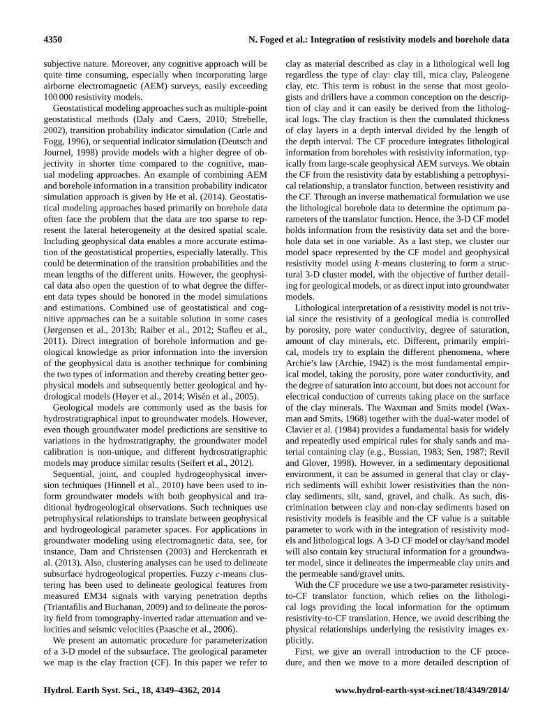
Horizontal slices of the 3-D cluster model are shown inFig. 9. The near-surface parts of the model (Fig. 9a, b) aredominated by clusters 2 and 4, while the deeper parts of themodel (Fig. 9c, d) are dominated by clusters 3 and 5, with the

east–west-striking buried valley to the south (Fig. 9c) primar-ily represented by clusters 1 and 2.

The histograms in Fig. 10 show how the original variables,the CF model, and the resistivity model are represented inthe five clusters. Clusters 3 and 5 have resistivity values al-most exclusively below 10�m and CF values above 0.7, butmostly close to 1. In the resistivity model space, clusters 2and 4 represent high and intermediate resistivity values, re-spectively, with some overlap, while cluster 1 overlaps withboth clusters 2 and 4. Figure 10 also clearly shows that boththe resistivity values and the CF values contribute to the fi-nal clusters. The clusters 1, 2, and 4 span only part of theresistivity space with significant overlaps (Fig. 10a), while



they are clearly separated in the CF model space and spanthe entire interval (Fig. 10b). The opposite is observed forclusters 3, 4, and 5, which are clearly separated in the resis-tivity space (Fig. 10a), but strongly overlap in the CF modelspace (Fig. 10b).

The CF model does not differentiate between clay types,in contrast to the EM resistivity data, which have a good res-olution in the low-resistivity range and are therefore able, tosome degree, to distinguish between clay types. This resultsin the two-part clustering of the low resistivity (> 20�m) val-ues as seen in Fig. 10a.

4 Discussion

4.1 Translator function, grid, and discretization

The spatially varying resistivity-to-CF translator functionis the key to achieving consistency between the boreholeinformation and the resistivity models, and the spatial varia-tions of the translator model account for, at least, two mainphenomena: (1) changes in the resistivity–lithology petro-physical relationship, and (2) the resolution capability in thegeophysical results.

The first issue includes spatial changes in the pore waterresistivity, the degree of water saturation, and/or contents ofclay minerals for the sediments described lithologically asclay. The spatial variation in the pore water resistivity on thismodeling scale is probably relatively smooth and small andwill therefore only have a minor impact on the resistivity-to-lithology/CF translation. Even in the case with larger fluctu-ations in the pore water resistivity (e.g., presence of salinepore water), the translator function will automatically adaptto this as long as we have borehole information available thatresembles the changes and the basic assumption that the clay-rich formations are more conductive than coarse-grained sed-iments is fulfilled.

In the Norsminde area used in the case history, the ground-water table is generally located a few meters below the sur-face and the groundwater is fresh. This means that the neitherpore water resistivity nor the water saturation plays a majorrole in the resistivity–clay-fraction relationship and thus thetranslator function. However, in the case with a thicker unsat-urated zone like for the pore water resistivity, the translatorfunction will automatically adapt to this situation as long asborehole information is available.

The varying content of clay minerals in the lithologies de-scribed as clay will effect the translator model. The correla-tion between the clay mineral content and resistivity is quitestrong and could be the key parameter instead of the simpleclay fraction of this procedure, but it would require clay min-eral content values available in boreholes on a large modelingscale, which is why we disregard this approach and use theintentionally simple definition of clay and clay fraction.

Figure 9. Horizontal slices in four depths of the 3-D cluster model.

The second issue concerns the resolution of the true for-mation resistivity in the resistivity models. Lithological logscontain point information with a good and uniform verti-cal resolution. In contrast, AEM data provide a good spatialcoverage, but the vertical resolution is relatively poor anddecreases with depth. Detailed geological layer sequencesmight only be represented by an average conductivity or onlyhave a weak signature in the resistivity models. By allowingspatial variation in the translation we can, to some degree,resolve weak layer indications in the resistivity models byutilizing the vertically detailed structural information fromthe lithological logs via the translator function.

The resolution in the final CF model is strongly correlatedto the resolution in the resistivity model, since the resistiv-ity data set contributes the majority of the information. Ingeneral, EM methods are sensitive to absolute changes in theelectric conductivity, which makes the resolution in the low-resistivity end superior to the resolution of high-resistivitycontrasts. The diffusive behavior of EM methods resultsin a decreasing horizontal and vertical resolution capabilitywith depth, and the vertical resolution capability furthermorestrongly depends on the layer sequence. A sequence of thinlithological layering may therefore be represented as a singleresistivity layer with an average conductivity, which is obvi-ously challenging for the geological interpretation. The hor-izontal resolution strongly depends on the sample/line den-sity of the geophysical measurements, but the footprint ofa single measurement sets the lower limit for the horizontalresolution. The Norsminde airborne SkyTEM survey is con-ducted with a very dense line spacing, giving a very high



Figure 10.Cluster statistics. The histograms show which data fromthe original variables make up the five clusters.(a) The distributionof the resistivity data in the five clusters.(b) The distribution of theCF data in the five clusters.

lateral resolution, which could actually support a finer hori-zontal discretization (25–50 m) in the CF model. The 100 mhorizontal discretization of the CF model and cluster modelwas selected to match the computational grid setup of a sub-sequent groundwater model. A detailed overview of resolu-tion capabilities of the Norsminde SkyTEM survey is givenby Schamper et al. (2014b), including an extensive compari-son to borehole data.

The horizontal sampling of the translator function shouldin principle be able to reproduce the true (but unknown) vari-ations in the resistivity-to-CF translation. However, it is pri-marily the borehole density and secondarily the complexityof the petrophysical relationship between clay and resistivitythat dictate the needed horizontal sampling of the transla-tor function. In our experience, a horizontal discretization ofthe translator function grid of 1–2 km (linearly interpolatedbetween nodes) is sufficient to obtain an acceptable consis-tency between the lithological logs and the translated resis-tivities. For the deeper part of the model domain where theborehole information is sparse, a coarser translator functiongrid would be sufficient.

Starting model values for the translator function in theinversion scheme become important in areas with very lowborehole density, primarily the deeper part of the model do-main. The starting model values are selected based on experi-ence and by visual comparison of the resistivity models withkey lithological logs. The horizontal and vertical constraintsmigrate information from regions with many boreholes to re-gions with few or no boreholes. As in most inversion tasks, afew initial inversions are performed to fine-tune and evaluatethe effect of different starting models and constraint setups.

The CF procedure supports both uncertainty estimates onthe input data, on the output translator functions, and on thefinal CF model. Generally, the uncertainties in the CF modelare closely related to the borehole density and quality, as wellas resolution and density of the resistivity models. The cal-culation and estimation of input and output uncertainties isdescribed in detail in Christiansen et al. (2014).

4.2 Clustering and validation

For the clustered 3-D model, each cluster represents someunit with fairly uniform characteristics. It could be hydro-stratigraphic units where the hydraulic conductivity of thecluster units is determined through a subsequent ground-water model calibration, typically constrained by hydrologi-cal head and discharge data. Groundwater model calibrationof the Norsminde 3-D cluster model has been performed witha preliminary positive outcome, but more experiments areneeded before drawing final conclusions. In this process oneneeds to evaluate the cluster validity, i.e., how many clustersthe data can support. Cluster validity can be assessed withvarious statistical measures (e.g., Halkidi et al., 2002). Thenumber of clusters resulting in the best hydrological perfor-mance might also be used as a measure of cluster validity.The validity of the clusters and the resulting groundwatermodel is still to be explored in more detail.

5 Conclusions

We have presented a procedure to produce 3-D clay fraction(CF) models, integrating the key sources of information in awell-documented and objective way.

The CF procedure combines lithological borehole in-formation with geophysical resistivity models in produc-ing large-scale 3-D clay fraction models. The integrationof the lithological borehole data and the resistivity mod-els is accomplished through inversion, where the optimumresistivity-to-CF function minimizes the difference betweenthe observed clay fraction from boreholes and the clay frac-tion found through the geophysical resistivity models. TheCF procedure allows for horizontal and lateral variation inthe resistivity-to-CF translation with smoothness constraintsas regularization. The spatially varying translator functionis the key to achieving consistency between the borehole



information and the resistivity models. The CF procedurefurthermore handles uncertainties in both input and outputdata.

The CF procedure was applied to a 156 km2 survey withmore than 700 boreholes and 100 000 resistivity models froman airborne survey. The output was a detailed 3-D clay frac-tion model combining resistivity models and lithologicalborehole information into one parameter.

Finally a cluster analysis was applied to achieve a pre-defined number of geological/hydrostratigraphic clusters inthe 3-D model and enabled us to integrate various sourcesof information, both geological and geophysical. The finalfive-cluster model differentiates between clay materials anddifferent high-resistivity materials from information held inresistivity model and borehole observations, respectively.

With the CF procedure and clustering we aim to build 3-Dmodels suitable as structural input for groundwater models.Each cluster will then represent a hydrostratigraphic unit andthe hydraulic conductivity of the units will be determinedthrough the groundwater model calibration constrained byhydrological head and discharge data.

The 3-D clay fraction model can also be seen as a binomialgeological sand–clay model by interpreting the high and lowCF values as clay and sand, respectively, as the color scale forthe CF model example in Figs. 7 and 8 indicates. Integrationand further development of the CF model into more-complexgeological models have been carried out with success (Jør-gensen et al., 2013b).

Acknowledgements.The research for this paper was carried outwithin the STAIR3-D project (funded by Geocenter Denmark) andthe HyGEM project (funded by the Danish Council for StrategicResearch under contract no. DSF 11-116763). We are also gratefulfor the support provided through the NiCA research project (fundedby the Danish Council for Strategic Research under contract no.DSF 09-067260), which allowed us access to the SkyTEM datafor the Norsminde case, and wish to thank Claus Ditlefsen, senioradvisor at the Geological Survey of Denmark and Greenland(GEUS), for his work and help with quality rating of the boreholedata. Finally, we extend our great thanks to our colleagues, toCasper Kirkegaard for help with optimization of the numericalcode, and to Professor Emeritus Niels Bøie Christensen forinsightful comments on the uncertainty migration.

Edited by: M. Giudici

References

Archie, G. E.: The electrical resistivity log as an aid in determiningsome reservoir characteristics, Trans. AIME, 146, 54–62, 1942.

Auken, E. and Christiansen, A. V.: Layered and laterally constrained2-D inversion of resistivity data, Geophysics, 69, 752–761, 2004.

Auken, E., Christiansen, A. V., Jacobsen, B. H., Foged, N., andSørensen, K. I.: Piecewise 1-D Laterally Constrained Inversionof resistivity data, Geophys. Prospect., 53, 497–506, 2005.

Auken, E., Christiansen, A. V., Westergaard, J. A., Kirkegaard, C.,Foged, N., and Viezzoli, A.: An integrated processing scheme forhigh-resolution airborne electromagnetic surveys, the SkyTEMsystem, Explor. Geophys., 40, 184–192, 2009.

Auken, E., Christiansen, A. V., Kirkegaard, C., Fiandaca, G.,Schamper, C., Behroozmand, A. A., Binley, A., Nielsen, E., Ef-fersø, F., Christensen, N. B., Sørensen, K. I., Foged, N., andVignoli, G.: An overview of a highly versatile forward andstable inverse algorithm for airborne, ground-based and bore-hole electromagnetic and electric data, Explor. Geophys., 1–13,doi:10.1071/EG13097, 2014.

Bussian, A. E.: Electrical conductance in a porous medium, Geo-physics, 48, 1258–1268, 1983.

Carle, S. F. and Fogg, G. E.: Transition Probability-Based IndicatorGeostatistics, Mathematical Geology, 28, 453–476, 1996.

Christiansen, A. V. and Auken, E.: A global measure for depth ofinvestigation, Geophysics, 77, 4, WB171–WB177, 2012.

Christiansen, A. V., Foged, N., and Auken, E.: A concept for cal-culating accumulated clay thickness from borehole lithologicallogs and resistivity models for nitrate vulnerability assessment,J. Appl. Geophys., 108, 69–77, 2014.

Clavier, C., Coates, G., and Dumanoir, J.: Theoretical and experi-mental bases for the dual-water model for interpretation of shalysands, Soc. Petrol. Eng. J., 24, 153–168, 1984.

Daly, C. and Caers, J. K.: Multi-point geostatistics – an introductoryoverview, First Break, 28, 39–47, 2010.

Dam, D. and Christensen, S.: Including geophysical data in groundwater model inverse calibration, Ground Water, 41, 178–189,2003.

Deutsch, C. V. and Journel, A. G.: GSLIB: geostatistical software li-brary and user’s guide, Second edition, Oxford University Press,1998.

Geonics Limited,http://www.geonics.com/index.html(last acces:29 October 2014), 2012.

Halkidi, M., Batistakis, Y., and Vazirgiannis, M.: Clustering validitychecking methods: Part II, Sigmod Record, 31, 19–27, 2002.

Härdle, K. W. and Simar, L.: Applied Multivariate Statistical Anal-ysis, Springer, 2012.

He, X., Koch, J., Sonnenborg, T. O., Jørgensen, F., Scham-per, C., and Refsgaard, J. C.: Transition probability basedstochastic geological modeling using airborne geophysicaldata and borehole data: Water Resour. Res., Special Issueon Patterns in Soil-Vegetation-Atmosphere Systems, Mon-itoring, Modeling and Data Assimilation, 50, 3147–3169,doi:10.1002/2013WR014593, 2014.

Herckenrath, D., Fiandaca, G., Auken, E., and Bauer-Gottwein,P.: Sequential and joint hydrogeophysical inversion using afield-scale groundwater model with ERT and TDEM data, Hy-drol. Earth Syst. Sci., 17, 4043–4060, doi:10.5194/hess-17-4043-2013, 2013.

Hinnell, A. C., Ferre, T. P. A., Vrugt, J. A., Huisman, J. A.,Moysey, S., Rings, J., and Kowalsky, M. B.: Improved extrac-tion of hydrologic information from geophysical data throughcoupled hydrogeophysical inversion, Water Resour. Res., 46,doi:10.1029/2008WR007060, 2010.

Hotelling, H., Analysis of a complex of statistical variables intoprincipal components, J. Educ. Psychol., 24, 417–441, 1933.

Høyer, A.-S., Jørgensen, F., Lykke-Andersen, H., and Christiansen,A. V.: Iterative modelling of AEM data based on geological a


http://dx.doi.org/10.1071/EG13097

http://www.geonics.com/index.html

http://dx.doi.org/10.1002/2013WR014593

http://dx.doi.org/10.5194/hess-17-4043-2013


http://dx.doi.org/10.1029/2008WR007060


priori information from seismic and borehole data, Near Surf.Geophys., 12, 635–650, doi:10.3997/1873-0604.2014024, 2014.

Jørgensen, F. and Sandersen, P. B. E.: Buried and open tunnel val-leys in Denmark-erosion beneath multiple ice sheets, QuaternarySci. Rev., 25, 1339–1363, 2006.

Jørgensen, F., Scheer, W., Thomsen, S., Sonnenborg, T. O., Hinsby,K., Wiederhold, H., Schamper, C., Burschil, T., Roth, B., Kirsch,R., and Auken, E.: Transboundary geophysical mapping of geo-logical elements and salinity distribution critical for the assess-ment of future sea water intrusion in response to sea level rise,Hydrol. Earth Syst. Sci., 16, 1845–1862, doi:10.5194/hess-16-1845-2012, 2012.

Jørgensen, F., Møller, R. R., Nebel, L., Jensen, N., Christiansen,A. V., and Sandersen, P.: A method for cognitive 3-D geologicalvoxel modelling of AEM data, B. Eng. Geol. Environ., 72, 421–432, doi:10.1007/s10064-013-0487-2, 2013a.

Jørgensen, F., Sandersen, P. B. E., Høyer, A.-S., Pallesen, T. M.,Foged, N., He, X., and Sonnenborg, T. O.: A 3-D geologicalmodel from Jutland, Denmark, Combining modeling techniquesto address variations in data density, data type, and geology, TheGeological Society of America, 125th Anniversary Annual Meet-ing, Denver, Colorado, USA, 2013b.

Møller, I., Verner, H., Søndergaard, V. H., Flemming, J., Auken, E.,and Christiansen, A. V.: Integrated management and utilizationof hydrogeophysical data on a national scale, Near Surf. Geo-phys., 7, 647–659, 2009.

Paasche, H.,Tronicke, J., Holliger, K., Green, A. G., and Maurer,H.: Integration of diverse physical-property models: Subsurfacezonation and petrophysical parameter estimation based on fuzzyc means cluster analyses, Geophysics, 71, H33–H44, 2006.

Pebesma, E. J. and C. G. Wesseling: Gstat: A Program for geosta-tistical Modelling, Prediction and Simultation, Comput. Geosci.,24, 17–31, 1998.

Raiber, M., White, P. A., Daughney, C. J., Tschritter, C., Davidson,P., and Bainbridge, S. E.: Three-dimensional geological mod-elling and multivariate statistical analysis of water chemistrydata to analyse and visualise aquifer structure and groundwa-ter composition in the Wairau Plain, Marlborough District, NewZealand, J. Hydrol., 48, 436–437, 2012.

Rasmussen, E. S., Dybkjær, K., and Piasecki, S.: Lithostratigraphyof the upper Oligocene – Miocene succession of Denmark, Geol.Surv. Den. Greenl., 22, 1–92, 2010.

Refsgaard, A., Auken, E., Bamberg, C. A., Christensen, B. S. B.,Clausen, T., Dalgaard, E., Effersø, F., Ernstsen, V., Gertz, F.,Hansen, A. L., He, X., Jacobsen,B. H., Jensen, K. H., Jørgensen,F., Jørgensen, L. F., Koch, J., Nilsson, B., Petersen, C., DeSchep-per, G., Schamper, C., Sørensen, K. I., Therrien, R., Thirup, C.,and Viezzoli, A.: Nitrate reduction in geologically heterogeneouscatchments – A framework for assessing the scale of predic-tive capability of hydrological models, ScienceDirect, 468–469,1278–1288, 2014.

Revil, A. and Glover, P. W. J.: Nature of surface electrical con-ductivity in natural sands, sandstones, and clays, Geophys. Res.Lett., 25, 691–694, 1998.

Sandersen, P., Jørgensen, F., Larsen, N. K., Westergaard, J. H., andAuken, E.: Rapid tunnel-valley formation beneath the recedingLate Weichselian ice sheet in Vendsyssel, Denmark, Boreas, 38,834–851, doi:10.1111/j.1502-3885.2009.00105.x, 2009.

Schamper, C., Auken, E., and Sørensen, K. I.: Coil responseinversion for very early time modelling of helicopter-bornetime-domain electromagnetic data and mapping of near-surface geological layers, Geophys. Prospect., 62, 658–674,doi:10.1111/1365-2478.12104, 2014a.

Schamper, C., Jørgensen, F., Auken, E., and Effersø, F.: As-sessment of near-surface mapping capabilities by airbornetransient electromagnetic data – An extensive comparisonto conventional borehole data, Geophysics, 79, B187–B199,doi:10.1190/geo2013-0256.1, 2014b.

Seifert, D., Sonnenborg, T. O., Refsgaard, J. C., Højberg, A. L., andTroldborg, L.: Assessment of hydrological model predictive abil-ity given multiple conceptual geological models: Water Resour.Res., 48, W06503, doi:10.1029/2011WR011149, 2012.

Sen, P. N.: Electrochemical origin of conduction in shaly forma-tions: Society of Petroleum Engineers, Presented at 62nd AnnualTechnical Conference and Exhibition, 1987.

Slater, L.: Near surface electrical characterization of hydraulic con-ductivity: From petrophysical properties to aquifer geometries –A review, Surv. Geophys., 28, 169–197, 2007.

Stafleu, J., Maljers, D., Gunnink, J. L., Menkovic, A., and Bussch-ers, F. S.: 3-D modelling of the shallow subsurface of Zeeland,the Netherlands: Geologie en Mijnbouw/Netherlands, J. Geosci.,90, 293–310, 2011.

Strebelle, S.: Conditional simulation of complex geological struc-tures using multiple-point statistics, Math. Geol., 34, 1–21, 2002.

Triantafilis, J. and Buchanan, S. M.: Identifying common near-surface and subsurface stratigraphic units using EM34 signaldata and fuzzyk means analysis in the Darling River valley, Aust.J. Earth Sci., 56, 535–558, 2009.

Turner, A.: Challenges and trends for geological modelling and vi-sualisation, B. Eng. Geol. Environ., 65, 109–127, 2006.

Viezzoli, A., Christiansen, A. V., Auken, E., and Sørensen, K. I.:Quasi-3-D modeling of airborne TEM data by Spatially Con-strained Inversion, Geophysics, 73, F105–F113, 2008.

Waxman, M. H. and Smits, L. J. M.: Electrical Conductivities inOil-Bearing Shaly Sands, Society of Petroleum Engineers Jour-nal, 8, 107–122, 1968.

Wisén, R., Auken, E., and Dahlin, T.: Combination of 1-D later-ally constrained inversion and 2-D smooth inversion of resistiv-ity data with a priori data from boreholes, Near Surf. Geophys.,3, 71–79, 2005.

Wu, J.: Advances ink means Clustering: A Data Mining Thinking,Springer, 2012.


http://dx.doi.org/10.3997/1873-0604.2014024



http://dx.doi.org/10.1007/s10064-013-0487-2

http://dx.doi.org/10.1111/j.1502-3885.2009.00105.x

http://dx.doi.org/10.1111/1365-2478.12104

http://dx.doi.org/10.1190/geo2013-0256.1

http://dx.doi.org/10.1029/2011WR011149

large-scale 3-d modeling by integration of resistivity ...hgg.au.dk/fileadmin/ · pdf...

Documents