laplace approximation in high-dimensional bayesian regression · r.f. barber, m. drton, k.m....
TRANSCRIPT
Laplace approximation in high-dimensional
Bayesian regression
Rina Foygel Barber
Department of StatisticsThe University of ChicagoChicago, IL 60637, U.S.A.e-mail: [email protected]
Mathias Drton
Department of StatisticsUniversity of WashingtonSeattle, WA 98195, U.S.A.
e-mail: [email protected]
and
Kean Ming Tan
Department of BiostatisticsUniversity of WashingtonSeattle, WA 98195, U.S.A.e-mail: [email protected]
Abstract: We consider Bayesian variable selection in sparse high-dimensional regres-sion, where the number of covariates p may be large relative to the sample size n, butat most a moderate number q of covariates are active. Specifically, we treat generalizedlinear models. For a single fixed sparse model with well-behaved prior distribution, clas-sical theory proves that the Laplace approximation to the marginal likelihood of themodel is accurate for sufficiently large sample size n. We extend this theory by givingresults on uniform accuracy of the Laplace approximation across all models in a high-dimensional scenario in which p and q, and thus also the number of considered models,may increase with n. Moreover, we show how this connection between marginal likeli-hood and Laplace approximation can be used to obtain consistency results for Bayesianapproaches to variable selection in high-dimensional regression.
Keywords and phrases: Bayesian inference, generalized linear models, Laplace ap-proximation, logistic regression, model selection, variable selection.
1. Introduction
A key issue in Bayesian approaches to model selection is the evaluation of the marginallikelihood, also referred to as the evidence, of the different models that are being considered.While the marginal likelihood may sometimes be available in closed form when adoptingsuitable priors, most problems require approximation techniques. In particular, this is thecase for variable selection in generalized linear models such as logistic regression, which arethe models treated in this paper. Different strategies to approximate the marginal likelihoodare reviewed by Friel and Wyse (2012). Our focus will be on the accuracy of the Laplaceapproximation that is derived from large-sample theory; see also Bishop (2006, Section 4.4).
Suppose we have n independent observations of a response variable, and along with eachobservation we record a collection of p covariates. Write L(β) for the likelihood function of
1
arX
iv:1
503.
0833
7v1
[m
ath.
ST]
28
Mar
201
5
R.F. Barber, M. Drton, K.M. Tan/Laplace approximation in high-dimensional regression 2
a generalized linear model relating the response to the covariates, where β ∈ Rp is a vectorof coefficients in the linear predictor (McCullagh and Nelder, 1989). Let f(β) be a prior
distribution, and let β be the maximum likelihood estimator (MLE) of the parameter vectorβ ∈ Rp. Then the evidence for the (saturated) regression model is the integral∫
Rp
L(β)f(β) dβ,
and the Laplace approximation is the estimate
Laplace := L(β)f(β)
((2π)p
detH(β)
)1/2
,
where H denotes the negative Hessian of the log-likelihood function logL.Classical asymptotic theory for large sample size n but fixed number of covariates p shows
that the Laplace approximation is accurate with high probability (Haughton, 1988). With pfixed, this then clearly also holds for variable selection problems in which we would considerevery one of the finitely many models given by the 2p subsets of covariates. This accuracyresult justifies the use of the Laplace approximation as a proxy for an actual model evidence.The Laplace approximation is also useful for proving frequentist consistency results aboutBayesian methods for variable selection for a general class of priors. This is again discussedin Haughton (1988). The ideas go back to the work of Schwarz (1978) on the Bayesianinformation criterion (BIC).
In this paper, we set out to give analogous results on the interplay between Laplace ap-proximation, model evidence, and frequentist consistency in variable selection for regressionproblems that are high-dimensional, possibly with p > n, and sparse in that we consideronly models that involve small subsets of covariates. We denote q as an upper bound on thenumber of active covariates. In variable selection for sparse high-dimensional regression, thenumber of considered models is very large, on the order of pq. Our interest is then in boundson the approximation error of Laplace approximations that, with high probability, hold uni-formly across all sparse models. Theorem 1, our main result, gives such uniform bounds (seeSection 3). A numerical experiment supporting the theorem is described in Section 4.
In Section 5, we show that when adopting suitable priors on the space of all sparse models,model selection by maximizing the product of model prior and Laplace approximation isconsistent in an asymptotic scenario in which p and q may grow with n. As a corollary, weobtain a consistency result for fully Bayesian variable selection methods. We note that theclass of priors on models we consider is the same as the one that has been used to defineextensions of BIC that have consistency properties for high-dimensional variable selectionproblems (see, for example, Bogdan, Ghosh and Doerge, 2004; Chen and Chen, 2008; Zak-Szatkowska and Bogdan, 2011; Chen and Chen, 2012; Frommlet et al., 2012; Luo and Chen,2013; Luo, Xu and Chen, 2015; Barber and Drton, 2015). The prior has also been discussedby Scott and Berger (2010).
2. Setup and assumptions
In this section, we provide the setup for the studied problem and the assumptions neededfor our results.

R.F. Barber, M. Drton, K.M. Tan/Laplace approximation in high-dimensional regression 3
2.1. Problem setup
We treat generalized linear models for n independent observations of a response, which wedenote as Y1, . . . , Yn. Each observation Yi follows a distribution from a univariate exponentialfamily with density
pθ(y) ∝ exp {y · θ − b(θ)} , θ ∈ R,
where the density is defined with respect to some measure on R. Let θi be the (natural)parameter indexing the distribution of Yi, so Yi ∼ pθi . The vector θ = (θ1, . . . , θn)T is thenassumed to lie in the linear space spanned by the columns of a design matrix X = (Xij) ∈Rn×p, that is, θ = Xβ for a parameter vector β ∈ Rp. Our work is framed in a settingwith a fixed/deterministic design X. In the language of McCullagh and Nelder (1989), ourbasic setup uses a canonical link, no dispersion parameter and an exponential family whosenatural parameter space is the entire real line. This covers, for instance, logistic and Poissonregression. However, extensions beyond this setting are possible; see for instance the relatedwork of Luo and Chen (2013) whose discussion of Bayesian information criteria encompassesother link functions.
We write Xi for the ith row of X, that is, the p-vector of covariate values for observation Yi.The regression model for the responses then has log-likelihood, score, and negative Hessianfunctions
logL(β) =
n∑i=1
Yi ·XTi β − b(XT
i β) ∈ R ,
s(β) =
n∑i=1
Xi
(Yi − b′(XT
i β))∈ Rp ,
H(β) =
n∑i=1
XiXTi · b′′(XT
i β) ∈ Rp×p .
The results in this paper rely on conditions on the Hessian H, and we note that, implicitly,these are actually conditions on the design X.
We are concerned with a sparsity scenario in which the joint distribution of Y1, . . . , Ynis determined by a true parameter vector β0 ∈ Rp supported on a (small) set J0 ⊂ [p] :={1, . . . , p}, that is, β0j 6= 0 if and only if j ∈ J0. Our interest is in the recovery of the setJ0 when knowing an upper bound q on the cardinality of J0, so |J0| ≤ q. To this end, weconsider the different submodels given by the linear spaces spanned by subsets J ⊂ [p] of thecolumns of the design matrix X, where |J | ≤ q.
For notational convenience, we take J ⊂ [p] to mean either an index set for the covariatesor the resulting regression model. The regression coefficients in model J form a vector oflength |J |. We index such vectors β by the elements of J , that is, β = (βj : j ∈ J), andwe write RJ for the Euclidean space containing all these coefficient vectors. This way thecoefficient and the covariate it belongs to always share a common index. In other words, thecoefficient for the j-th coordinate of covariate vector Xi is denoted by βj in any model Jwith j ∈ J . Furthermore, it is at times convenient to identify a vector β ∈ RJ with the vectorin Rp that is obtained from β by filling in zeros outside of the set J . As this is clear from thecontext, we simply write β again when referring to this sparse vector in Rp. Finally, sJ(β)and HJ(β) denote the subvector and submatrix of s(β) and H(β), respectively, obtained byextracting entries indexed by J . These depend only on the subvectors XiJ = (Xij)j∈J of thecovariate vectors Xi.
R.F. Barber, M. Drton, K.M. Tan/Laplace approximation in high-dimensional regression 4
2.2. Assumptions
Recall that n is the sample size, p is the number of covariates, q is an upper bound on themodel size, and β0 is the true parameter vector. We assume the following conditions to holdfor all considered regression problems:
(A1) The Euclidean norm of the true signal is bounded, that is, ‖β0‖2 ≤ a0 for a fixedconstant a0 ∈ (0,∞).
(A2) There is a decreasing function clower : [0,∞) → (0,∞) and an increasing functioncupper : [0,∞) → (0,∞) such that for all J ⊂ [p] with |J | ≤ 2q and all β ∈ RJ , theHessian of the negative log-likelihood function is bounded as
clower(‖β‖2)IJ �1
nHJ(β) � cupper(‖β‖2)IJ .
(A3) There is a constant cchange ∈ (0,∞) such that for all J ⊂ [p] with |J | ≤ 2q and allβ, β′ ∈ RJ ,
1
n‖HJ(β)−HJ(β′)‖sp ≤ cchange · ‖β − β′‖2,
where ‖ · ‖sp is the spectral norm of a matrix.
Assumption (A2) provides control of the spectrum of the Hessian of the negative log-likelihood function, and (A3) yields control of the change of the Hessian. Together, (A2) and(A3) imply that for all ε > 0, there is a δ > 0 such that
(1− ε)HJ(β0) � HJ(βJ) � (1 + ε)HJ(β0), (2.1)
for all J ⊇ J0 with |J | ≤ 2q and βJ ∈ RJ with ‖βJ − β0‖2 ≤ δ; see Prop. 2.1 in Barber andDrton (2015). Note also that we consider sets J with cardinality 2q in (A2) and (A3) becauseit allows us to make arguments concerning false models, with J 6⊇ J0, using properties of thetrue model given by the union J ∪ J0.
Remark 2.1. When treating generalized linear models, some control of the size of the truecoefficient vector β0 is indeed needed. For instance, in logistic regression, if the norm ofβ0 is too large, then the binary response will take on one of its values with overwhelmingprobability. Keeping with the setting of logistic regression, Barber and Drton (2015) showhow assumptions (A2) and (A3) hold with high probability in certain settings in which thecovariates are generated as i.i.d. sample. Assumptions (A2) and (A3), or the implicationfrom (2.1), also appear in earlier work on Bayesian information criteria for high-dimensionalproblems such as Chen and Chen (2012) or Luo and Chen (2013).
Let {fJ : J ⊂ [p], |J | ≤ q} be a family of probability density functions fJ : RJ → [0,∞)that we use to define prior distributions in all q-sparse models. We say that the family islog-Lipschitz with respect to radius R > 0 and has bounded log-density ratios if there existtwo constants F1, F2 ∈ [0,∞) such that the following conditions hold for all J ⊂ [p] with|J | ≤ q:
(B1) The function log fJ is F1-Lipschitz on the ball BR(0) = {β ∈ RJ : ‖β‖2 ≤ R}, i.e., forall β′, β ∈ BR(0), we have
| log fJ(β′)− log fJ(β)| ≤ F1‖β′ − β‖2.
(B2) For all β ∈ RJ ,log fJ(β)− log fJ(0) ≤ F2.
R.F. Barber, M. Drton, K.M. Tan/Laplace approximation in high-dimensional regression 5
Example 2.1. If we take fJ to be the density of a |J |-fold product of a centered normaldistribution with variance σ2, then (B1) holds with F1 = R/σ2 and F2 = 0.
3. Laplace approximation
This section provides our main result. For a high-dimensional regression problem, we showthat a Laplace approximation to the marginal likelihood of each sparse model,
Evidence(J) :=
∫RJ
L(β)fJ(β)dβ ,
leads to an approximation error that, with high probability, is bounded uniformly across allmodels. To state our result, we adopt the notation
a = b(1± c) :⇐⇒ a ∈ [b(1− c), b(1 + c)].
Theorem 1. Suppose conditions (A1)–(A3) hold. Then, there are constants ν, csample, aMLE ∈(0,∞) depending only on (a0, clower, cupper, cchange) such that if
n ≥ csample · q3 max{log(p), log3(n)},
then with probability at least 1 − p−ν the following two statements are true for all sparsemodels J ⊂ [p], |J | ≤ q:
(i) The MLE βJ satisfies ‖βJ‖2 ≤ aMLE.
(ii) If additionally the family of prior densities {fJ : J ⊂ [p], |J | ≤ q} satisfies the Lipschitzcondition from (B1) for radius R ≥ aMLE + 1, and has log-density ratios bounded as in (B2),then there is a constant cLaplace ∈ (0,∞) depending only on (a0, clower, cupper, cchange, F1, F2)such that
Evidence(J) = L(βJ)fJ(βJ) ·
((2π)|J|
detHJ(βJ)
)1/2
·
1± cLaplace
√|J |3 log3(n)
n
.
Proof. (i) Bounded MLEs. It follows from Barber and Drton (2015, Sect. B.2)1 that, with
the claimed probability, the norms ‖βJ‖2 for true models J (i.e., J ⊇ J0 and |J | ≤ 2q) arebounded by a constant. The result makes reference to an event for which all the claims wemake subsequently are true. The bound on the norm of an MLE of a true model was obtainedby comparing the maximal likelihood to the likelihood at the true parameter β0. As we shownow, for false sparse models, we may argue similarly but comparing to the likelihood at 0.
Recall that a0 is the bound on the norm of β0 assumed in (A1) and that the functions clower
and cupper in (A2) are decreasing and increasing in the norm of β0, respectively. Throughoutthis part, we use the abbreviations
clower := clower(a0), cupper := cupper(a0).
1In the proof of this theorem, we cite several results from Barber and Drton (2015, Sect. B.2, Lem. B.1).Although that paper treats the specific case of logistic regression, by examining the proofs of their resultsthat we cite here, we can see that they hold more broadly for the general GLM case as long as we assumethat the Hessian conditions hold, i.e., Conditions (A1)–(A3), and therefore we may use these results for thesetting considered here.

R.F. Barber, M. Drton, K.M. Tan/Laplace approximation in high-dimensional regression 6
First, we lower-bound the likelihood at 0 via a Taylor-expansion using the true model J0.For some t ∈ [0, 1], we have that
logL(0)− logL(β0) = −βT0 sJ0(β0)− 1
2βT0 HJ0(tβ0)β0 ≥ −βT0 sJ0(β0)− 1
2na20cupper,
where we have applied (A2). Lemma B.1 in Barber and Drton (2015) yields that
|βT0 sJ0(β0)| ≤ ‖HJ0(β0)−12 sJ0(β0)‖‖HJ0(β0)
12 β0‖ ≤ τ0a0
√ncupper,
where τ20 can be bounded by a constant multiple of q log(p). By our sample size assumption(i.e., the existence of the constant csample), we thus have that
logL(0)− logL(β0) ≥ −n · c1 (3.1)
for some constant c1 ∈ (0,∞).Second, we may consider the true model J ∪ J0 instead of J and apply (B.17) in Barber
and Drton (2015) to obtain the bound
logL(βJ)− logL(β0) ≤
‖βJ − β0‖ ·(√ncupper · τJ\J0 −
nclower
4min
{‖βJ − β0‖,
clower
2cchange
}), (3.2)
where τ2J\J0 can be bounded by a constant multiple of q log(p). Choosing our sample size
constant csample large enough, we may deduce from (3.2) that there is a constant c2 ∈ (0,∞)such that
logL(βJ)− logL(β0) ≤ −n‖βJ − β0‖c2
whenever ‖βJ −β0‖ > clower/(2cchange). Using the fact that logL(0) ≤ log(βJ) for any modelJ , we may deduce from (3.2) that there is a constant c2 ∈ (0,∞) such that
logL(0)− logL(β0) ≤ −n‖βJ − β0‖c2
whenever ‖βJ − β0‖ > clower/(2cchange). Together with (3.1), this implies that ‖βJ − β0‖ is
bounded by a constant c3. Having assumed (A1), we may conclude that the norm of βJ isbounded by a0 + c3.
(ii) Laplace approximation. Fix J ⊂ [p] with |J | ≤ q. In order to analyze the evidence ofmodel J , we split the integration domain RJ into two regions, namely, a neighborhood N ofthe MLE βJ and the complement RJ\N . More precisely, we choose the neighborhood of theMLE as
N :={β ∈ RJ : ‖HJ(βJ)1/2(β − βJ)‖2 ≤
√5|J | log(n)
}.
Then the marginal likelihood, Evidence(J), is the sum of the two integrals
I1 =
∫NL(β)fJ(β)dβ,
I2 =
∫RJ\N
L(β)fJ(β)dβ.

R.F. Barber, M. Drton, K.M. Tan/Laplace approximation in high-dimensional regression 7
We will estimate I1 via a quadratic approximation to the log-likelihood function. Outside ofthe region N , the quadratic approximation may no longer be accurate but due to concavity of
the log-likelihood function, the integrand can be bounded by e−c‖βJ−βJ‖2 for an appropriatelychosen constant c, which allows us to show that I2 is negligible when n is sufficiently large.
We now approximate I1 and I2 separately. Throughout this part we assume that we havea bound aMLE on the norms of the MLEs βJ in sparse models J with |J | ≤ q. For notationalconvenience, we now let
clower := clower(aMLE), cupper := cupper(aMLE).
(ii-a) Approximation of integral I1. By a Taylor-expansion, for any β ∈ RJ there is at ∈ [0, 1] such that
logL(β) = logL(βJ)− 1
2(β − βJ)THJ
(βJ + t(β − βJ)
)(β − βJ).
By (A3) and using that |t| ≤ 1,∥∥∥HJ
(βJ + t(β − βJ)
)−HJ(βJ)
∥∥∥sp≤ n · cchange ‖β − βJ‖2.
Hence,
logL(β) = logL(βJ)− 1
2(β − βJ)THJ(βJ)(β − βJ)± 1
2‖β − βJ‖32 · n cchange. (3.3)
Next, observe that (A2) implies that
HJ(βJ)−1/2 �√
1
nclower· IJ .
We deduce that for any vector β ∈ N ,
‖β − βJ‖2 ≤√
5|J | log(n) ‖HJ(βJ)−1/2‖sp ≤
√5|J | log(n)
nclower. (3.4)
This gives
logL(β) = logL(βJ)− 1
2(β − βJ)THJ(βJ)(β − βJ)±
√|J |3 log3(n)
n·
√125c2change
4c3lower
. (3.5)
Choosing the constant csample large enough, we can ensure that the upper bound in (3.4)
is no larger than 1. In other words, ‖β − βJ‖2 ≤ 1 for all points β ∈ N . By our assumption
that ‖βJ‖2 ≤ aMLE, the set N is thus contained in the ball
B ={β ∈ RJ : ‖β‖2 ≤ aMLE + 1
}.
Since, by (B1), the logarithm of the prior density is F1-Lipschitz on B, it follows form (3.4)that
log fJ(β) = log fJ(βJ)± F1‖β − βJ‖2 = log fJ(βJ)± F1
√5|J | log(n)
nclower. (3.6)
R.F. Barber, M. Drton, K.M. Tan/Laplace approximation in high-dimensional regression 8
Plugging (3.5) and (3.6) into I1, and writing a = b · exp{±c} to denote a ∈ [b · e−c, b · ec],we find that
I1 = L(βJ)fJ(βJ) exp
±√|J |3 log3(n)
n·
√ 5F 21
nclower+
√125c2change
4c3lower
×∫N
exp
{−1
2(β − βJ)THJ(βJ)(β − βJ)
}dβ.
(3.7)
In the last integral, change variables to ξ = HJ(βJ)1/2(β − βJ) to see that∫N
exp
{−1
2(β − βJ)THJ(βJ)(β − βJ)
}dβ
=(
detHJ(βJ))−1/2
·∫‖ξ‖2≤
√5|J| log(n)
exp
{−1
2‖ξ‖22
}dξ
=
((2π)|J|
detHJ(βJ)
)1/2
· Pr{χ2|J| ≤ 5|J | log(n)
}
=
((2π)|J|
detHJ(βJ)
)1/2
· exp{±1/√n}, (3.8)
where we use a tail bound for the χ2-distribution stated in Lemma A.1. We now substi-tute (3.8) into (3.7), and simplify the result using that e−x ≥ 1− 2x and ex ≤ 1 + 2x for all0 ≤ x ≤ 1. We find that
I1 = L(βJ)fJ(βJ)
((2π)|J|
detHJ(βJ)
)1/21± 2
1 +
√125c2change
4c3lower
+
√5F 2
1
clower
√ |J |3 log3(n)
n
(3.9)
when the constant csample is chosen large enough.
(ii-b) Approximation of integral I2. Let β be a point on the boundary of N . It then holdsthat
(β − βJ)THJ(βJ)(β − βJ) =√
5|J | log(n) · ‖HJ(βJ)1/2(β − βJ)‖2.
We may deduce from (3.5) that
logL(β) ≤ logL(βJ)−√
5|J | log(n)
2‖HJ(βJ)1/2(β − βJ)‖2 +
√|J |3 log3(n)
n·
√125c2change
4c3lower
≤ logL(βJ)− ‖HJ(βJ)1/2(β − βJ)‖2 ·√|J | log(n),
for |J |3 log3(n)/n sufficiently small, which can be ensured by choosing csample large enough.The concavity of the log-likelihood function now implies that for all β 6∈ N we have
logL(β) ≤ logL(βJ)− ‖HJ(βJ)1/2(β − βJ)‖2 ·√|J | log(n). (3.10)
Moreover, using first assumption (B2) and then assumption (B1), we have that
log fJ(β) ≤ log fJ(0) + F2 ≤ log fJ(βJ) + F1‖βJ‖2 + F2.

R.F. Barber, M. Drton, K.M. Tan/Laplace approximation in high-dimensional regression 9
Since ‖βJ‖2 ≤ aMLE, it thus holds that
log fJ(β) ≤ log fJ(βJ) + F1aMLE + F2. (3.11)
Combining the bounds from (3.10) and (3.11), the integral can be bounded as
I2 ≤ L(βJ)fJ(βJ)eF1aMLE+F2 ·∫RJ\N
exp{−‖HJ(βJ)1/2(β − βJ)‖2 ·
√|J | log(n)
}dβ.
(3.12)
Changing variables to ξ = HJ(βJ)1/2(β − βJ) and applying Lemma A.2, we may bound theintegral in (3.12) as∫
RJ\Nexp
{−‖HJ(βJ)1/2(β − βJ)‖2 ·
√|J | log(n)
}dβ
≤(
detHJ(βJ))−1/2
·∫‖ξ‖2>
√5|J| log(n)
exp{−√|J | log(n) · ‖ξ‖2
}dξ
≤(
detHJ(βJ))−1/2
· 4(π)|J|/2
Γ(12 |J |
) √5|J | log(n)|J|−1√
|J | log(n)e−√5 |J| log(n)
=
((2π)|J|
detHJ(βJ)
)1/2
· 2√
5
Γ(12 |J |
) (5
2|J | log(n)
)|J|/2−1· 1
n√5 |J|
.
Stirling’s lower bound on the Gamma function gives
(|J |/2)|J|/2−1
Γ(12 |J |
) =(|J |/2)|J|/2
Γ(12 |J |+ 1
) ≤ 1√|J |π
e|J|/2.
Using this inequality, and returning to (3.12), we see that
I2 ≤ L(βJ)fJ(βJ)
((2π)|J|
detHJ(βJ)
)1/2
× eF1aMLE+F2 · 2e√
5√|J |π
·(
5e log(n)
n
)|J|/2−11
n(√5−1/2)·|J|+1
. (3.13)
Based on this fact, we certainly have the very loose bound that
I2 ≤ L(βJ)fJ(βJ)
((2π)|J|
detHJ(βJ)
)1/2
eF1aMLE+F2 · 1√n, (3.14)
for all sufficiently large n.
(ii-c) Combining the bounds. From (3.9) and (3.14), we obtain that
Evidence(J) = I1 + I2 = L(βJ)fJ(βJ)
((2π)|J|
detHJ(βJ)
)1/2
×1±
eF1aMLE+F2 + 2 +
√125c2changec3lower
+
√20F 2
1
clower
√ |J |3 log3(n)
n
(3.15)
for sufficiently large n, as desired.
R.F. Barber, M. Drton, K.M. Tan/Laplace approximation in high-dimensional regression 10
Remark 3.1. The proof of Theorem 1 could be modified to handle other situations of interest.For instance, instead of a fixed Lipschitz constant F1 for all log prior densities, one couldconsider the case where log fJ is Lipschitz with respect to a constant F1(J) that growswith the cardinality of |J |, e.g., at a rate of
√|J | in which case the rate of square root of
|J |3 log3(n)/n could be modified to square root of |J |4 log3(n)/n. The term eF1(J)aMLE thatwould appear in (3.15) could be compensated using (3.13) in less crude of a way than whenmoving to (3.14).
4. Numerical experiment for sparse Bayesian logistic regression
In this section, we perform a simulation study to assess the approximation error in Laplaceapproximations to the marginal likelihood of logistic regression models. To this end, wegenerate independent covariate vectors X1, . . . , Xn with i.i.d. N(0, 1) entries. For each choiceof a (small) value of q, we take the true parameter vector β0 ∈ Rp to have the first qentries equal to two and the rest of the entries equal zero. So, J0 = {1, . . . , q}. We thengenerate independent binary responses Y1, . . . , Yn, with values in {0, 1} and distributed as(Yi|Xi) ∼ Bernoulli(pi(Xi)), where
pi(x) =
(exp
(xTβ0
)1 + exp (xTβ0)
)⇐⇒ log
(pi(x)
1− pi(x)
)= x · β0,
based on the usual (and canonical) logit link function.We record that the logistic regression model with covariates indexed by J ⊂ [p] has the
likelihood function
L(β) = exp
{n∑i=1
Yi ·XTiJβ − log
(1 + exp(XT
iJβ))}
, β ∈ RJ , (4.1)
where, as previously defined, XiJ = (Xij)j∈J denotes the subset of covariates for model J .The negative Hessian of the log-likelihood function is
HJ(β) =
n∑i=1
XiJXTiJ ·
exp(XTiJβ)(
1 + exp(XTiJβ)
)2 .For Bayesian inference in the logistic regression model given by J , we consider as a priordistribution a standard normal distribution on RJ , that is, the distribution of a random vectorwith |J | independentN(0, 1) coordinates. As in previous section, we denote the resulting priordensity by fJ . We then wish to approximate the evidence or marginal likelihood
Evidence(J) :=
∫RJ
L(β)fJ(β) dβ.
As a first approximation, we use a Monte Carlo approach in which we simply draw inde-pendent samples β1, . . . , βB from the prior fJ and estimate the evidence as
MonteCarlo(J) =1
B
B∑b=1
L(βb),

R.F. Barber, M. Drton, K.M. Tan/Laplace approximation in high-dimensional regression 11
02
46
8
Number of Samples, n
Lapl
ace
Appr
oxim
atio
n Er
ror
50 60 70 80 90 100
● ● ● ● ● ●
● q=1q=2q=3
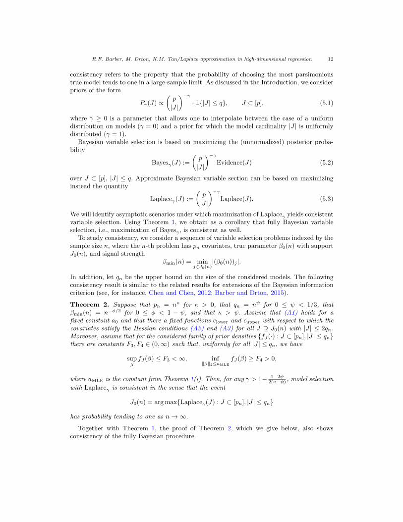
Fig 1. Maximum Laplace approximation error, averaged over 100 data sets, as a function of the samplesize n. The number of covariates is n/2, and the number of active covariates is bounded by q ∈ {1, 2, 3}.
where we use B = 50, 000 in all of our simulations. As a second method, we compute theLaplace approximation
Laplace(J) := L(βJ)fJ(βJ)
((2π)|J|
detHJ(βJ)
)1/2
,
where βJ is the maximum likelihood estimator in model J . For each choice of the number ofcovariates p, the model size q, and the sample size n, we calculate the Laplace approximationerror as
maxJ⊂[p], |J|≤q
| log MonteCarlo(J)− log Laplace(J) | .
We consider n ∈ {50, 60, 70, 80, 90, 100} in our experiment. Since we wish to compute theLaplace approximation error of every q-sparse model, and the number of possible models ison the order of pq, we consider p = n/2 and q ∈ {1, 2, 3}. The Laplace approximation error,averaged across 100 independent simulations, is shown in Figure 1. We remark that the errorin the Monte Carlo approximation to the marginal likelihood is negligible compared to thequantity plotted in Figure 1. With two independent runs of our Monte Carlo integrationroutine, we found the Monte Carlo error to be on the order of 0.05.
For each q = 1, 2, 3, Figure 1 shows a decrease in Laplace approximation error as nincreases. We emphasize that p and thus also the number of considered q-sparse modelsincrease with n. As we increase the number of active covariates q, the Laplace approximationerror increases. These facts are in agreement with Theorem 1. This said, the scope of thissimulation experiment is clearly limited by the fact that only small values of q and moderatevalues of p and n are computationally feasible.
5. Consistency of Bayesian variable selection
In this section, we apply the result on uniform accuracy of the Laplace approximation (The-orem 1) to prove a high-dimensional consistency result for Bayesian variable selection. Here,
R.F. Barber, M. Drton, K.M. Tan/Laplace approximation in high-dimensional regression 12
consistency refers to the property that the probability of choosing the most parsimonioustrue model tends to one in a large-sample limit. As discussed in the Introduction, we considerpriors of the form
Pγ(J) ∝(p
|J |
)−γ· 1{|J | ≤ q}, J ⊂ [p], (5.1)
where γ ≥ 0 is a parameter that allows one to interpolate between the case of a uniformdistribution on models (γ = 0) and a prior for which the model cardinality |J | is uniformlydistributed (γ = 1).
Bayesian variable selection is based on maximizing the (unnormalized) posterior proba-bility
Bayesγ(J) :=
(p
|J |
)−γEvidence(J) (5.2)
over J ⊂ [p], |J | ≤ q. Approximate Bayesian variable section can be based on maximizinginstead the quantity
Laplaceγ(J) :=
(p
|J |
)−γLaplace(J). (5.3)
We will identify asymptotic scenarios under which maximization of Laplaceγ yields consistentvariable selection. Using Theorem 1, we obtain as a corollary that fully Bayesian variableselection, i.e., maximization of Bayesγ , is consistent as well.
To study consistency, we consider a sequence of variable selection problems indexed by thesample size n, where the n-th problem has pn covariates, true parameter β0(n) with supportJ0(n), and signal strength
βmin(n) = minj∈J0(n)
|(β0(n))j |.
In addition, let qn be the upper bound on the size of the considered models. The followingconsistency result is similar to the related results for extensions of the Bayesian informationcriterion (see, for instance, Chen and Chen, 2012; Barber and Drton, 2015).
Theorem 2. Suppose that pn = nκ for κ > 0, that qn = nψ for 0 ≤ ψ < 1/3, thatβmin(n) = n−φ/2 for 0 ≤ φ < 1 − ψ, and that κ > ψ. Assume that (A1) holds for afixed constant a0 and that there a fixed functions clower and cupper with respect to which thecovariates satisfy the Hessian conditions (A2) and (A3) for all J ⊇ J0(n) with |J | ≤ 2qn.Moreover, assume that for the considered family of prior densities {fJ(·) : J ⊂ [pn], |J | ≤ qn}there are constants F3, F4 ∈ (0,∞) such that, uniformly for all |J | ≤ qn, we have
supβfJ(β) ≤ F3 <∞, inf
‖β‖2≤aMLE
fJ(β) ≥ F4 > 0,
where aMLE is the constant from Theorem 1(i). Then, for any γ > 1− 1−2ψ2(κ−ψ) , model selection
with Laplaceγ is consistent in the sense that the event
J0(n) = arg max{Laplaceγ(J) : J ⊂ [pn], |J | ≤ qn}
has probability tending to one as n→∞.
Together with Theorem 1, the proof of Theorem 2, which we give below, also showsconsistency of the fully Bayesian procedure.
R.F. Barber, M. Drton, K.M. Tan/Laplace approximation in high-dimensional regression 13
Corollary 5.1. Under the assumptions of Theorem 2, fully Bayesian model selection isconsistent, that is, the event
J0(n) = arg max{Bayesγ(J) : J ⊂ [pn], |J | ≤ qn}
has probability tending to one as n→∞.
Proof of Theorem 2. Our scaling assumptions for pn, qn and βmin(n) are such that the con-ditions imposed in Theorem 2.2 of Barber and Drton (2015) are met for n large enough. Thistheorem and Theorem 1(i) in this paper then yield that there are constants ν, ε, Cfalse, aMLE >0 such that with probability at least 1−pνn the following three statements hold simultaneously:
(a) For all |J | ≤ qn with J ⊇ J0(n),
log L(βJ)− log L(βJ0(n)) ≤ (1 + ε)(|J\J0(n)|+ ν) log(pn) . (5.4)
(b) For all |J | ≤ qn with J 6⊃ J0(n),
log L(βJ0(n))− log L(βJ) ≥ Cfalse nβmin(n)2 . (5.5)
(c) For all |J | ≤ qn and some constant aMLE > 0,
‖βJ‖ ≤ aMLE. (5.6)
In the remainder of this proof we show that these three facts, in combination with furthertechnical results from Barber and Drton (2015), imply that
J0(n) = arg max{Laplaceγ(J) : J ⊂ [pn], |J | ≤ qn}. (5.7)
For simpler notation, we no longer indicate explicitly that pn, qn, β0 and derived quantitiesvary with n. We will then show that
logLaplaceγ(J0)
Laplaceγ(J)= (logP (J0)− logP (J)) +
(logL(βJ0)− logL(βJ)
)− |J\J0| log
√2π
+(
log fJ0(βJ0)− log fJ(βJ))
+1
2
(log detHJ(βJ)− log detHJ0(βJ0)
)(5.8)
is positive for any model given by a set J 6= J0 of cardinality |J | ≤ q. We let
clower := clower(aMLE), cupper := cupper(aMLE).
False models. If J 6⊇ J0, that is, if the model is false, we observe that
logP (J0)− logP (J) = −γ log
(p
|J0|
)+ γ log
(p
|J |
)≥ −γ log
(p
|J0|
)≥ −γq log p.
Moreover, by (A2) and (5.6),
log detHJ(βJ)− log detHJ0(βJ0) ≥ |J | · log(nclower)− |J0| · log(ncupper)
≥ −q log
(n
cuppermin{clower, 1}
).

R.F. Barber, M. Drton, K.M. Tan/Laplace approximation in high-dimensional regression 14
Combining the lower bounds with (5.5), we obtain that
logLaplaceγ(J0)
Laplaceγ(J)≥ Cfalsenβ
2min − |J\J0| log(
√2π)− q log
(pγn
cuppermin{clower, 1}
)+ log
(F4
F3
)≥ Cfalsenβ
2min − q log
(cupper
min{clower, 1}·√
2πnpγ)
+ log
(F4
F3
).
By our scaling assumptions, the lower bound is positive for sufficiently large n.
True models. It remains to resolve the case of J ) J0, that is, when model J is true.We record that from the proof of Theorem 2.2 in Barber and Drton (2015), it holds on theconsidered event of probability at least 1− p−ν that for any J ⊇ J0,
‖βJ − β0‖2 ≤4√cupper√nclower
τ|J\J0|, (5.9)
where
τ2r =2
(1− ε′)3·[(J0 + r) log
(3
ε′
)+ log(4pν) + r log(2p)
].
Under our scaling assumptions on p and q, it follows that ‖βJ−β0‖2 tends to zero as n→∞.We begin again by considering the prior on models, for which we have that
logP (J0)− logP (J) = γ log|J0|!(p− |J0|)!|J |!(p− |J |)!
≥ −γ|J\J0| log q + γ|J\J0| log(p− q)
≥ −γ|J\J0| log q + γ|J\J0|(1− ε) log p
for all n sufficiently large. Indeed, we assume that p = nκ and q = nψ with κ > ψ such thatp− q ≥ p1−ε for any small constant ε > 0 as long as p is sufficiently large relative to q.
Next, if J ) J0, then (A2) and (A3) allow us to relate HJ(βJ) and HJ0(βJ0) to therespective Hessian at the true parameter, i.e., HJ(β0) and HJ0(β0). We find that
log
(detHJ(βJ)
detHJ0(βJ0)
)≥ log
(detHJ(β0)
detHJ0(β0)
)+ |J | log
(1− cchange
clower‖βJ − β0‖2
)− |J0| log
(1 +
cchangeclower
‖βJ0 − β0‖2).
Note that by assuming n large enough, we may assume that ‖βJ − β0‖2 and ‖βJ0 − β0‖2are small enough for the logarithms to be well defined; recall (5.9). Using that x ≥ log(1 +x) for all x > −1 and log(1− x
2 ) ≥ −x for all 0 ≤ x ≤ 1, we see that
log
(detHJ(βJ)
detHJ0(βJ0)
)≥ log
(detHJ(β0)
detHJ0(β0)
)− 2|J |cchange
clower‖βJ − β0‖2
− |J0|cchangeclower
‖βJ0 − β0‖2.
Under our scaling assumptions, q3 log(p) = o(n), and thus applying (5.9) twice shows that
−2|J |cchangeclower
‖βJ − β0‖2 − |J0|cchangeclower
‖βJ0 − β0‖2
R.F. Barber, M. Drton, K.M. Tan/Laplace approximation in high-dimensional regression 15
is larger than any small negative constant for n large enough. For simplicity, we take thelower bound as −1. By (A2), it holds that
log
(detHJ(β0)
detHJ0(β0)
)= log det
(HJ\J0(β0)−HJ0,J\J0(β0)THJ0(β0)−1HJ0,J\J0(β0)
)≥ |J\J0| log(n) + |J\J0| log(clower),
because the eigenvalues of the Schur complement of HJ(β0) are bounded the same way asthe eigenvalues of HJ(β0); see, e.g., Chapter 2 of Zhang (2005). Hence, for sufficiently largen, the following is true for all J ) J0:
log detHJ(βJ)− log detHJ0(βJ0) ≥ |J\J0| log(n) + |J\J0| log(clower)− 1. (5.10)
Combining the bound for the model prior probabilities with (5.4) and (5.10), we have forany true model J ) J0 that
logLaplaceγ(J0)
Laplaceγ(J)
≥ −(1 + ε)(|J\J0|+ ν) log(p) + γ|J\J0|(1− ε) log(p) +1
2|J\J0| log(n)
− γ|J\J0| log(q) +1
2|J\J0|
(log
clower
2π
)+ log
(F4
F3
)− 1
≥ 1
2|J\J0|
(log(n)− log q2γ + 2 [(1− ε)γ − (1 + ε)(1 + ν)] log(p) + log
(clower
2π
))+ log
(F4
F3
)− 1.
This lower bound is is positive for all n large because our assumption that p = nκ, q = nψ
for 0 ≤ ψ < 1/3, and
γ > 1− 1− 2ψ
2(κ− ψ)
implies that
limn→∞
√n
p(1+ε)(1+ν)−γ(1−ε)qγ=∞ (5.11)
provided the constants ε, ν, and ε are chosen sufficiently small.
6. Discussion
In this paper, we have shown that in the context of high-dimensional variable selectionproblems, the Laplace approximation can be accurate uniformly across a potentially verylarge number of sparse models. We then showed how this approximation result allows one togive results on the consistency of fully Bayesian techniques for variable selection.
In practice, it is of course infeasible to evaluate the evidence or Laplace approximation forevery single sparse regression model, and some search strategy must be adopted instead. Somerelated numerical experiments can be found in Chen and Chen (2008), Chen and Chen (2012),Zak-Szatkowska and Bogdan (2011), and Barber and Drton (2015), although that workconsiders BIC scores that drop some of the terms appearing in the Laplace approximation.
Finally, we emphasize that the setup we considered concerns generalized linear modelswithout dispersion parameter and with canonical link. The conditions from Luo and Chen(2013) could likely be used to extend our results to other situations.

R.F. Barber, M. Drton, K.M. Tan/Laplace approximation in high-dimensional regression 16
References
Anderson, T. W. (2003). An introduction to multivariate statistical analysis, third ed. Wi-ley Series in Probability and Statistics. Wiley-Interscience [John Wiley & Sons], Hoboken,NJ. MR1990662 (2004c:62001)
Barber, R. F. and Drton, M. (2015). High-dimensional Ising model selection withBayesian information criteria. Electronic Journal of Statistics 9 567–607.
Bishop, C. M. (2006). Pattern recognition and machine learning. Information Science andStatistics. Springer, New York. MR2247587 (2007c:62002)
Bogdan, M., Ghosh, J. K. and Doerge, R. (2004). Modifying the Schwarz Bayesianinformation criterion to locate multiple interacting quantitative trait loci. Genetics 167989–999.
Chen, J. and Chen, Z. (2008). Extended Bayesian information criteria for model selectionwith large model spaces. Biometrika 95 759–771. MR2443189
Chen, J. and Chen, Z. (2012). Extended BIC for small-n-large-P sparse GLM. Statist.Sinica 22 555–574. MR2954352
Friel, N. and Wyse, J. (2012). Estimating the evidence—a review. Stat. Neerl. 66 288–308.MR2955421
Frommlet, F., Ruhaltinger, F., Twarog, P. and Bogdan, M. (2012). Modified ver-sions of Bayesian information criterion for genome-wide association studies. Comput.Statist. Data Anal. 56 1038–1051. MR2897552
Haughton, D. M. A. (1988). On the choice of a model to fit data from an exponentialfamily. Ann. Statist. 16 342–355. MR924875 (89e:62036)
Laurent, B. and Massart, P. (2000). Adaptive estimation of a quadratic functional bymodel selection. Ann. Statist. 28 1302–1338. MR1805785 (2002c:62052)
Luo, S. and Chen, Z. (2013). Selection consistency of EBIC for GLIM with non-canonicallinks and diverging number of parameters. Stat. Interface 6 275–284. MR3066691
Luo, S., Xu, J. and Chen, Z. (2015). Extended Bayesian information criterion in theCox model with a high-dimensional feature space. Ann. Inst. Statist. Math. 67 287–311.MR3315261
McCullagh, P. and Nelder, J. A. (1989). Generalized linear models. Monographson Statistics and Applied Probability. Chapman & Hall, London Second edition [ofMR0727836]. MR3223057
Natalini, P. and Palumbo, B. (2000). Inequalities for the incomplete gamma function.Math. Inequal. Appl. 3 69–77. MR1731915 (2001c:33006)
Schwarz, G. (1978). Estimating the dimension of a model. Ann. Statist. 6 461–464.MR0468014 (57 ##7855)
Scott, J. G. and Berger, J. O. (2010). Bayes and empirical-Bayes multiplicity adjustmentin the variable-selection problem. Ann. Statist. 38 2587–2619. MR2722450 (2011h:62268)
Zak-Szatkowska, M. and Bogdan, M. (2011). Modified versions of the Bayesian in-formation criterion for sparse generalized linear models. Comput. Statist. Data Anal. 552908–2924. MR2813055 (2012g:62313)
Zhang, F., ed. (2005). The Schur complement and its applications. Numerical Methods andAlgorithms 4. Springer-Verlag, New York. MR2160825 (2006e:15001)
Appendix A: Technical lemmas
This section provides two lemmas that were used in the proof of Theorem 1.
R.F. Barber, M. Drton, K.M. Tan/Laplace approximation in high-dimensional regression 17
Lemma A.1 (Chi-square tail bound). Let χ2k denote a chi-square random variable with k
degrees of freedom. Then, for any n ≥ 3,
P{χ2k ≤ 5k log(n)
}≥ 1− 1
nk≥ exp{−1/
√n}.
Proof. Since log(n) ≥ 1 when n ≥ 3, we have that
k + 2√k · k log(n) + 2k log(n) ≤ 5k log(n).
Using the chi-square tail bound in Laurent and Massart (2000), it thus holds that
P{χ2k ≤ 5k log(n)
}≥ P
{χ2k ≤ k + 2
√k · k log(n) + 2k log(n)
}≥ 1− e−k log(n).
Finally, for the last step, by the Taylor series for x 7→ ex, for all n ≥ 3 we have
exp{−1/√n} ≤ 1− 1√
n+
1
2· 1
n≤ 1− 1
n.
Lemma A.2. Let k ≥ 1 be any integer, and let a, b > 0 be such that ab ≥ 2(k − 1). Then∫‖ξ‖2>a
exp{−b‖ξ‖2}dξ ≤4(π)k/2
Γ(12k) ak−1
be−ab,
where the integral is taken over ξ ∈ Rk.
Proof. We claim that the integral of interest is∫‖ξ‖2>a
exp{−b‖ξ‖2}dξ =2(π)k/2
bkΓ(12k) ∫ ∞
r=ab
rk−1e−rdr. (A.1)
Indeed, in k = 1 dimension,∫‖ξ‖2>a
exp{−b‖ξ‖2}dξ = 2
∫ ∞r=a
e−brdr =2
be−ab,
which is what (A.1) evaluates to. If k ≥ 2, then using polar coordinates (Anderson, 2003,Exercises 7.1-7.3), we find that∫
‖ξ‖2>aexp{−b‖ξ‖2}dξ = 2π
∫ ∞r=a
rk−1e−brdr ·k−2∏i=1
∫ π/2
−π/2cosi(θi)dθi
= 2π
∫ ∞r=a
rk−1e−brdr ·k−2∏i=1
√π Γ
(12 (i+ 1)
)Γ(12 (i+ 2)
) ,
which again agrees with the formula from (A.1).Now, the integral on the right-hand side of (A.1) defines the upper incomplete Gamma
function and can be bounded as
Γ(k, ab) =
∫ ∞r=ab
rk−1e−rdr ≤ 2e−ab(ab)k−1
for ab ≥ 2(k− 1); see inequality (3.2) in Natalini and Palumbo (2000). This gives the boundthat was to be proven.