landscape indices as measures of the effects of fragmentation: can pattern …€¦ · ·...
TRANSCRIPT

Landscape indices as measures ofthe effects of fragmentation: canpattern reflect process?
DOC SCIENCE INTERNAL SERIES 98
Daniel Rutledge
Published by
Department of Conservation
PO Box 10-420
Wellington, New Zealand

DOC Science Internal Series is a published record of scientific research carried out, or advice given,
by Department of Conservation staff, or external contractors funded by DOC. It comprises progress
reports and short communications that are generally peer-reviewed within DOC, but not always
externally refereed. Fully refereed contract reports funded from the Conservation Services Levy (CSL)
are also included.
Individual contributions to the series are first released on the departmental intranet in pdf form.
Hardcopy is printed, bound, and distributed at regular intervals. Titles are listed in the DOC Science
Publishing catalogue on the departmental website http://www.doc.govt.nz and electronic copies of
CSL papers can be downloaded from http://www.csl.org.nz
© Copyright March 2003, New Zealand Department of Conservation
ISSN 1175�6519
ISBN 0�478�22380�3
In the interest of forest conservation, DOC Science Publishing supports paperless electronic
publishing. When printing, recycled paper is used wherever possible.
This report was prepared for publication by DOC Science Publishing, Science & Research Unit; editing
and layout by Helen O�Leary. Publication was approved by the Manager, Science & Research Unit,
Science Technology and Information Services, Department of Conservation, Wellington.

CONTENTS
Abstract 5
1. Introduction 6
2. Ecosystem fragmentation: concept and consequences 7
2.1 What is fragmentation and what is ecosystem fragmentation? 7
2.2 Effects of fragmentation 9
2.2.1 Effects on abiota 9
2.2.2 Effects on biota 9
3. Landscape indices used to characterise fragmentation 10
3.1 Composition 11
3.2 Shape 13
3.3 Configuration 14
3.3.1 Distance-based configuration indices 16
3.3.2 Pattern-based configuration indices 17
4. Landscape indices and ecosystem fragmentation:
what do we know? 18
5. Conclusions 20
6. Future research 22
7. Acknowledgements 24
8. References 24

5DOC Science Internal Series 98
© March 2003, New Zealand Department of Conservation. This paper may be cited as:
Rutledge, D. 2003: Landscape indices as measures of the effects of fragmentation: can pattern reflect
process? DOC Science Internal Series 98. Department of Conservation, Wellington. 27 p.
Landscape indices as measures ofthe effects of fragmentation: canpattern reflect process?
Daniel Rutledge
Landcare Research, Private Bag 3127, Hamilton, New Zealand
A B S T R A C T
This review examines landscape indices and their usefulness in reflecting the
effects of ecosystem fragmentation. Rapid fragmentation of natural ecosystems
by anthropogenic activity spurred the development of landscape indices, which
occurred in three phases. In proliferation, indices were introduced to quantify
aspects of fragmentation, including composition, shape, and configuration. In
re-evaluation, several studies demonstrated that landscape indices vary with
varying landscape attributes, correlate highly with one another, and relate
differently to different processes. Finally, in re-direction, efforts shifted towards
developing new or modified indices motivated by ecological theory or
incorporating pattern directly into models of ecological process.
Overall, landscape indices do not serve as useful indicators of fragmentation
effects. While certain indices are useful in specific cases, most indices should
only be used to describe landscape pattern. Research should develop
knowledge and models of ecosystem processes that incorporate fragmentation
directly. Potential research areas include area requirements of different
processes, understanding when patterns of fragmentation are important and
when not, understanding which processes operate at which scales, determining
relationships between pattern and exotic species persistence, and evaluating
the effects of different levels of information on pattern and any follow-on
effects. Studying processes directly will provide the information required to
choose among various conservation options to maximize conservation gains.
Keywords: configuration, connectivity, ecosystem, fragmentation, habitat,
landscape, landscape indices, pattern, process, shape, viability
6 Rutledge�Landscape indices as measures of the effects of fragmentation
1. Introduction
Since their arrival in New Zealand nearly 1000 years ago, humans have
substantially changed its landscape. Natural ecosystems have been replaced by
man-made ecosystems or altered through the introduction of many non-native
species. Indigenous forests have declined from an estimated 81% to 23% of total
land area and remain mostly in upland areas with steeper slopes. Tussock and
scrub have increased from 12% to 23% of total land area, including large
expanses of the exotic scrub gorse (Ulex europaeus). Non-native ecosystems,
including croplands, pastures, plantation forests, and urban areas now
comprise approximately 45% of New Zealand�s land area (Leathwick et al. in
press). These changes alter the conditions in which native species live,
including but not limited to the amount, distribution, and availability of
resources; the presence of new competitors or predators; the loss of co-evolved
species; and the distribution of social networks.
In addition to a decrease in total area, most natural ecosystems have also been
partitioned or fragmented into (often many) smaller pieces. The remaining
pieces, typically called �patches� or �fragments�, can vary in a number of ways.
First, they can vary in number. Theoretically the number of patches could be
unlimited, but in practice the number of patches is limited by: the definition of
a patch; the size or extent of the study area; and the resolution of the study unit.
Second, they can vary in distribution of sizes, ranging from one very large patch
and a number of much smaller patches, to a uniform distribution where each
patch is roughly the same size. Third, they can vary in shape, ranging from
simple shapes such as paddocks to highly complex and convoluted shapes such
as riparian areas. Fourth, they can vary in spatial configuration in terms of their
position relative to similar patches and dissimilar patches. For example,
remaining areas of indigenous forest range from relatively large patches found
within the conservation estate to very small patches on private land scattered
throughout agricultural areas.
The loss and fragmentation of indigenous ecosystems presents a formidable
challenge to conservation management, given that both the resulting patterns
and their effects on different ecological processes vary considerably.
Furthermore, these patterns and effects change over time and at varying rates
(Turner 1989). Given limited time and resources, there is a need to identify and
understand general relationships between patterns and processes, particularly
those that result from human activities.
Having recognized such a need, the amount of research on pattern and process
and the interactions between them has grown over the past 20 years. One area
receiving considerable attention has been the development of indices to
measure landscape pattern (Hargis et al. 1997, 1998; Tischendorf 2001). If
pattern does affect process, then indices of landscape pattern may correlate
with ecological processes and could provide a means to detect and monitor
ecological changes. This is particularly important given the recognition that
conservation management must occur over broad spatial and temporal scales
and that most natural ecosystems now occupy much smaller and fragmented
areas when compared with their former distributions.

7DOC Science Internal Series 98
This review assesses the state of knowledge concerning landscape indices and,
in particular, whether those indices can measure or indicate the effects of
fragmentation on ecosystems. It is organized into five sections: a broad
overview of fragmentation and its consequences; a description of fragmentation
indices, including a discussion of their benefits and drawbacks; a brief history of
the development of fragmentation indices; conclusions about the usefulness of
fragmentation indices for conservation management; and possible future
research directions.
This review does not attempt to do several things. First, it does not constitute
an exhaustive study of all fragmentation indices developed to date. There are
simply too many. Second, it does not provide an in-depth evaluation of the
mathematical properties of the indices presented. Instead, this review tries to
focus mostly on their use and relevance to ecological processes. Third, it does
not give much attention to the very real problem of the calculation, use, and
interpretation of landscape indices in a polygon (vector) environment versus a
grid (raster) environment. Those issues are best left to the user when dealing
with a particular index.
2. Ecosystem fragmentation:concept and consequences
2 . 1 W H A T I S F R A G M E N T A T I O N A N D W H A T I S
E C O S Y S T E M F R A G M E N T A T I O N ?
Fragmentation is an intuitive concept and involves dividing something into a
number of smaller pieces. Fragmentation is characterised by the number and
size distribution of the resulting pieces. A plate that is broken into 100 pieces is
more fragmented than a plate broken into 10 pieces. Similarly, a plate broken
into 10 pieces of equal size is more fragmented than a plate broken into 10
pieces, one of which is 90% of the original plate.
In an ecological sense, fragmentation involves dividing up contiguous
ecosystems into smaller areas called �patches.� A patch is an area having
relatively homogeneous conditions relative to other patches (Forman 1995).
The term �class� typically represents the different categories of possible
patches, e.g. land cover/land use classes, habitat classes, or vegetation classes.
Most often fragmentation implies the division of natural ecosystems into
smaller patches as the result of human activities, such as the development of
agricultural or urban areas in places once supporting forests or wetlands.
Fragmentation of an ecosystem will, by definition:
� Increase the number of patches
� Decrease the mean patch size
� Increase the total amount of edge, where edge is the border between patches
of two different classes

8 Rutledge�Landscape indices as measures of the effects of fragmentation
However, unlike the plate example given above, ecosystem fragmentation is
complicated in that the patches (or pieces) do not move. Historically,
fragmentation has occurred in conjunction with loss of area. Human activities
have also tended to simplify the shape and alter the configuration of remaining
patches of natural ecosystems. Consequently, the term �fragmentation� has been
applied broadly to all aspects of ecosystem change, including loss, composition
(number/size), shape, and configuration. For example, Forman (1995, p. 407)
defines fragmentation as follows:
The breaking up of a habitat or land type into smaller parcels, is here
considered as similar to the dictionary sense of breaking an object in
pieces. It is implicit that the pieces are somewhat-widely and usually
unevenly separated. Thus breaking a plate on the floor is fragmentation,
whereas carving up or subdividing an area with equal-width lines is
dissection.
Forman reflects the prevailing view that fragmentation includes other aspects
besides the number and size of patches, particularly the spatial configuration of
the resulting patches. Loss of area is implicit in his definition, although the
effects of loss of area should be separated out from effects of fragmentation.
Recently, studies have begun to partition the effects of loss and fragmentation
both theoretically (Fahrig 2001) and empirically (MacNally & Brown 2001;
MacNally & Horrocks 2002). Others have attempted to partition effects of shape
and configuration (Hargis et al. 1997; Huxel & Hastings 1999), but a strict
separation of the four aspects of ecosystem change is difficult given their
interrelationship.
It must be emphasized that the measurement of fragmentation depends on
patch definition and patch scale. Patch definition represents the set of possible
classes used to describe a particular area. Patches can represent ecosystems,
defined as areas containing a particular combination of abiotic and biotic
components, such as forest, wetlands, tussock, etc. Patches can represent the
generic concept of habitat, defined as areas containing resources needed by one
or more species of interest (Morrison et al. 1992; Hall et al. 1997). This results
in a binary (yes/no) classification of a landscape into habitat/non-habitat. Patch
definition often stems from an interpretation of the combined physical
attributes (e.g. land cover) and human activities (e.g. land use) occurring at a
given location. For example, the New Zealand Land Cover Database (Ministry
for the Environment 1997) has classes that indicate primarily land cover
(indigenous forest), a mixture of land cover and land use (plantation forest),
and primarily land use (urban). Increasing the number of classes will usually
increase fragmentation by creating more patches, whereas decreasing the
number of classes will decrease fragmentation as rarer land cover classes are
lost (Turner et al. 1989; Turner 1990).
Patch scale relates to the resolution of the study. Increasing resolution will
decrease the smallest patch size (e.g. one can detect smaller patches) and
probably increase the number of patches (Turner et al. 1989). Increasing
resolution will also affect measurement of patch area and patch edge, thus
affecting many landscape indices, particularly those related to shape (Benson &
MacKenzie 1995).

9DOC Science Internal Series 98
2 . 2 E F F E C T S O F F R A G M E N T A T I O N
Fragmentation affects ecosystems by altering the conditions within a patch and
the flow of resources (organisms, propagules, nutrients) among patches. As
discussed above, fragmentation occurs in conjunction with loss of area and
includes changes in composition, shape, and configuration of resulting patches.
What follows is a brief summary of the general effects of fragmentation on abiota
and biota. For a more comprehensive treatment, consult the following: Saunders
et al. (1991); Forman (1995); Harrison & Bruna (1999); Olff & Ritchie (2002).
2.2.1 Effects on abiota
Fragmenting an ecosystem alters the inputs and outputs of physical resources as
a function of the size, number, shape, and configuration of the resulting
patches. The level of effect often decreases along a gradient away from the
boundary of a patch towards the interior. To account for this relationship, a
patch is typically divided into �core� and �edge� areas (Morrison et al. 1992;
Forman 1995). Core areas lie at least a certain distance from the edge and tend
to have abiotic conditions similar to those found in the interior of larger
patches. Edge areas receive the most influence from neighbouring patches and
have a higher degree of alteration. Long and narrow patches may effectively
have no core area despite being quite large. The primary difficulty with the
core/edge model is that the distance used depends on the process of interest.
The abiotic conditions affected by fragmentation include light, moisture, wind,
and soil regimes (Saunders et al. 1991; Didham 1998). Within New Zealand, the
most relevant abiotic changes are those that occur in patches of indigenous
forest which once dominated the landscape and that now receive the highest
level of conservation effort. Fragmentation creates more forest edge, and the
new edge is often adjacent to patches with a more open physical structure such
as pasture or urban areas. The edge areas tend to receive more solar radiation.
Increased solar radiation can produce higher temperatures and drier conditions,
particularly when coupled with increased airflow from surrounding open areas.
The same processes can also affect soil conditions through heating and drying.
2.2.2 Effects on biota
Different species will respond differently to fragmentation. The differential
responses will restructure the ecological community within patches, often to a
state of lower species richness and high relative abundance of generalist species
(Harrison & Bruna 1999). Some changes will result from intraspecific processes
responding to changes in abiotic conditions. Other changes will result from
adjustments in interspecific interactions. Much study on fragmentation is
taxonomically oriented, with a high bias towards bird studies. Instead of a
taxonomic approach, it would be more fruitful to discuss the relationship
between fragmentation and biota in terms of the four, basic, intraspecific
population processes of growth, reproduction, mortality, and dispersal
(immigration and emigration) and the corresponding interspecific processes.
As abiotic conditions change, growth rates will change. Plant species
composition will change as competitive interactions cause reshuffling to reflect
changing abiotic conditions. The new plant species composition will affect

10 Rutledge�Landscape indices as measures of the effects of fragmentation
faunal species composition by determining which plant resources are available
to herbivores, which herbivores are available to predators, and what ends up
being recycled by detritivores. Animals may be forced to increase the size of
their home range to find enough resources to meet dietary needs, or their body
size may decrease as a consequence (Sumner et al. 1999). With fewer resources,
individuals may have fewer reserves for reproduction or combating parasites.
Conversely, edge areas may actually support more species because edge areas
tend to have attributes of both adjacent patches (Berry 2001).
Reproduction rates will change according to resource availability, mating
opportunities, and the density of herbivores/predators. Sometimes patches are
divided into sources and sinks; sources support self-sustaining populations
where rates of increase are ≥1 and sinks support populations but with rates of
increase <1 (Pulliam 1988). Changing abiotic conditions may affect seed
production, germination rates, and seedling survival. Animals may be smaller
owing to reduced food resources, which would make less energy available for
reproduction. Social structures may be disrupted and reduce the opportunity
for mating. Seeds or nests may be more vulnerable to predation by herbivores or
predators, respectively.
Mortality rates will vary according to resource availability, such as nutrients or
cover, or the presence/absence of a herbivore, predator, or competitor. At the
population level, an overall increase in mortality rate implies a greater risk of
extinction within the patch. Smaller patch sizes may increase mortality risk by
reducing the total area required for a predator to search or by increasing
visibility as individuals move between different patches. Conversely,
fragmentation may benefit certain species by providing a refuge if the predator
or disease has difficulty moving among patches.
Fragmentation often produces a series of isolated patches that remain
connected through dispersal. The theory of Island Biogeography (MacArthur &
Wilson 1967), which relates species persistence to island size and distance from
a colonization source, provides the underlying basis for the study of dispersal.
The traditional view is of the patch as habitat and the surrounding area or
�matrix� as inhospitable and often lethal (Haila 2002). A considerable amount of
research, both theoretical and empirical, has gone into understanding dispersal
among a network of patches. The salient message is that the effects vary widely
depending on the process or organism of interest. For example, species that
prefer core areas may avoid intervening areas altogether, effectively isolating
themselves (Pearson et al. 1996).
3. Landscape indices used tocharacterise fragmentation
Landscape indices broadly fall into one of two categories: non-spatial and spatial
(Gustafson 1998). Non-spatial indices describe landscape composition and
include measurements of the number of patch classes or proportions of total
11DOC Science Internal Series 98
area. Spatial indices describe patch attributes and contain information relevant
to measuring fragmentation. The spatial indices can be further divided into
those that describe patch composition, shape and configuration. In the strictest
sense, only patch composition relates to fragmentation, but the traditional view
of ecosystem fragmentation encompasses all three (as well as loss of area).
The major landscape indices for research on fragmentation were placed into the
three categories described above: composition (Table 1), shape (Table 2), and
configuration (Table 3). The decision to include an index in the table depended
on its treatment (or lack of treatment) in the literature and the amount of
original information it contained. Additional indices exist that are either related
to ones listed in the table or made available in software packages. FRAGSTATS,
for example, offers statistics at the patch, class, and landscape level (McCarigal
& Marks 1995; McCarigal et al. 2002). An index such as patch area can be
aggregated to report on mean patch area at the class or landscape level, but only
the index of patch area was included in the table. Several indices found in
FRAGSTATS appear to have little or no use in the literature, so were not listed in
the table.
The following discussion compares/contrasts the three categories of landscape
indices relevant to fragmentation.
3 . 1 C O M P O S I T I O N
Composition indices describe the basic characteristics of fragmentation. The
two basic indices used to quantify fragmentation are number of patches and
patch area, usually measured as mean patch area. However, they provide an
incomplete picture because the fragmentation concept also encompasses the
relative sizes of the pieces that result. Also, mean patch size is sensitive to the
addition or deletion of small patches. As a result, the largest patch index, which
measures the largest patch of a given class as a percentage of the total
landscape, is used to indicate relative size (With & King 1999; Saura & Martinez-
Millan 2001). These measures are affected by the resolution (Benson &
MacKenzie 1995) and extent of the study area. Patch density partly offsets this
problem by indicating the number of patches within a given area (usually 100)
and can, therefore, be used to compare different landscapes (McCarigal & Marks
1995; Saura & Martinez-Millan 2001).
The indices discussed above are measures of patch attributes and do not
necessarily have an ecological basis, although mean patch size and largest patch
index can be related to organism area requirements. A relatively new index
related to patch size is average patch carrying capacity (Vos et al. 2001).
Average patch carrying capacity scales patch size based on a species� area
requirements (Vos et al. 2001). It may provide a more meaningful measure of
patch size but will vary from one species to another. Also, the calculation for
species with large home ranges that encompass patches of habitat (e.g. areas
containing needed resources) and non-habitat (areas without such resources)
may prove difficult.

12 Rutledge�Landscape indices as measures of the effects of fragmentation
Jaeger (2000) has introduced two new indices that relate to patch composition:
splitting index and effective mesh size. Both are related to another index called
the degree of division index, which is a measure of aggregation within a
landscape. The splitting index relates to the number of patches and indicates
TABLE 1 . SELECTED LANDSCAPE INDICES MEASURING FRAGMENTATION COMPOSITION. SYMBOLS FOLLOW
AUTHORS� CONVENTION OR MCCARIGAL ET AL. (2002) . FOR DETAILED DESCRIPTIONS AND FORMULAE OF
LANDSCAPE INDICES, SEE RI ITTERS ET AL. (1995) AND MCCARIGAL ET AL. (2002) .
NAME SYMBOL VALUE 1 DESCRIPTION COMMENTS REFERENCE(S)
Number NP 1 ≤ NP ≤ Nmax Number of patches Depends on patch Turner et al. (1989)
of patches of a particular class definition and data
resolution
Mean patch MPS Amin< MPS ≤ Atot Average area of a Depends on data McCarigal et al. (2002)
size patch of a particular resolution; sensitiveclass to addition/deletion of
small patches
Largest patch LPI 0 < LPI ≤ 1 Percentage of Important for certain Forman (1995); With &
index landscape area ecological processes King (1999); Saura &
occupied by the Martinez-Millan (2001)
largest patch of a class
Patch density PD 0 < PD Number of patches of a Same as number of McCarigal & Marks
particular class per unit patches when (1995); Saura & Martinez-
area (standardized to comparing two Millan (2001)
100 ha in FRAGSTATS) landscapes of the
same size
Splitting S 0 < S ≤ Nmax Number of equal-sized Related to degree of Jaeger (2000)
index patches of a particular division (see Table 3)
class required to produce
a desired degree of
landscape division
Effective m Amin< m ≤ Atot Size of equal-area patch Related to degree of Jaeger (2000)
mesh size of a particular class division (see Table 3)
required to produce a
desired degree of
landscape division
Average Kavg 0 < Kavg< Kmax Average of the number Area depends on Vos et al. (2001)
patch of reproductive areas species of interest
carrying found in a patch based
capacity on the area needed
by a particular species
to reproduce
Core area CORE 0 ≤ CORE ≤ 1 Amount of area whose Specified distance varies McCarigal & Marks
boundary is a specified based on process or (1995); Schumaker
distance inwards from species of interest (1996)
the patch edge
Core area CAI 0 ≤ CAI ≤ 1 Percentage area of a Unitless; based on core McCarigal & Marks (1995)
index patch that is core area area and varies based
on process or species
of interest
1 Variables are defined as follows: Nmax = maximum possible number of patches, achieved when each patch has a minimum possible
area based on data resolution; Amin = minimum possible patch size based on data resolution; Atot = total area of a particular class; Kmax
= maximum number of reproductive areas if the entire landscape was suitable for reproduction by a particular species, e.g, total
landscape area divided by the area needed by a particular species to reproduce.

13DOC Science Internal Series 98
how many equal-sized patches produce a particular value of the degree of
division index. Effective mesh size relates to mean patch size and indicates what
size of equal-sized patches will produce a particular degree of division index.
Based on their mathematical properties, Jaeger claims that these new measures
are better than their counterparts, but those claims have not yet been
substantiated.
Two composition indices that are more ecologically based are core area and core
area index (McCarigal & Marks 1995; Schumaker 1996). As previously discussed,
core areas indicate interior areas of a patch which retain similar abiotic and biotic
conditions to pre-fragmented conditions and do not experience strong
influences from neighbouring patches. These indices measure core area, as
discussed earlier, and vary based on the relationship of patch size to patch shape
and the process of interest. In effect, they straddle the boundary between both
characteristics. Core area is a simple measurement of area, while core area index
is a ratio of core area to patch area (and hence unitless).
3 . 2 S H A P E
Shape indices attempt to quantify patch complexity, which can be important
for different ecological processes (Forman 1995). For example, circles or
squares will have less edge and, potentially, more core area. Other shapes�
such as long, narrow features like tree lines, or sinuous features like riparian
areas�may have comparatively little core area despite a large total area.
Compact areas may be less �visible� to species dispersing across the landscape,
while convoluted or linear shapes may intercept the paths of more organisms or
propagules (Forman 1995).
Most measures of patch shape focus on some variation of the perimeter-to-area
ratio (Krummel et al. 1987). More complex shapes will have a larger perimeter
or edge for a given area and therefore a higher perimeter:area ratio. The simple
ratio of perimeter:area suffers from a negative relationship with size, given the
same shape. For example, the perimeter:area ratio of a 4 × 4 square is 16/16 = 1,
while the perimeter:area ratio for a 10 × 10 square is 40/100 = 0.4 (Frohn 1998).
Shape index (McCarigal & Marks 1995; Patton 1975) overcomes size-
dependence by comparing the perimeter:area ratios to a standard shape such as
a square or circle. This removes the relationship with size but imposes the
restriction of choosing a reference shape.
Another index commonly used to characterise shape is fractal dimension
(Krummel et al. 1987; O�Neill, Krummel et al. 1988; Milne 1991). Fractal
dimension measures the degree of shape complexity. For images on a raster
(gridded) map, fractal dimension varies from 1, which indicates relatively
simple shapes such as squares, to 2, which indicates more complex and
convoluted shapes. The methods for calculating fractal dimension vary
depending upon the question or application. For landscape analysis, a common
method involves regressing the patch perimeters versus patch areas on a log:log
scale and relating the fractal dimension to the slope of the regression
(McCarigal & Marks 1995). Like shape index, fractal dimension measurements
are not affected by patch scale per se, e.g. a square of any size will have the
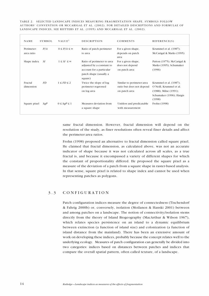
14 Rutledge�Landscape indices as measures of the effects of fragmentation
same fractal dimension. However, fractal dimension will depend on the
resolution of the study, as finer resolutions often reveal finer details and affect
the perimeter:area ratios.
Frohn (1998) proposed an alternative to fractal dimension called square pixel.
He claimed that fractal dimension, as calculated above, was not an accurate
indicator of shape because it was not calculated across all scales, as a true
fractal is, and because it encompassed a variety of different shapes for which
the constant of proportionality differed. He proposed the square pixel as a
measure of the deviation of a patch from a square shape in raster-based analysis.
In that sense, square pixel is related to shape index and cannot be used when
representing patches as polygons.
3 . 3 C O N F I G U R A T I O N
Patch configuration indices measure the degree of connectedness (Tischendorf
& Fahrig 2000b) or, conversely, isolation (Moilanen & Hanski 2001) between
and among patches on a landscape. The notion of connectivity/isolation stems
directly from the theory of Island Biogeography (MacArthur & Wilson 1967),
which relates species persistence on an island to a dynamic equilibrium
between extinction (a function of island size) and colonization (a function of
island distance from the mainland). There has been an extensive amount of
work on developing these indices, probably because the concept relates well to the
underlying ecology. Measures of patch configuration can generally be divided into
two categories: indices based on distances between patches and indices that
compare the overall spatial pattern, often called texture, of a landscape.
TABLE 2 . SELECTED LANDSCAPE INDICES MEASURING FRAGMENTATION SHAPE. SYMBOLS FOLLOW
AUTHORS� CONVENTION OR MCCARIGAL ET AL. (2002) . FOR DETAILED DESCRIPTIONS AND FORMULAE OF
LANDSCAPE INDICES, SEE RI ITTERS ET AL. (1995) AND MCCARIGAL ET AL. (2002) .
NAME SYMBOL VALUE 1 DESCRIPTION COMMENTS REFERENCE(S)
Perimeter: P/A 0 ≤ P/A ≤ ∞ Ratio of patch perimeter For a given shape, Krummel et al. (1987);
area ratio to area depends on patch McCarigal & Marks (1995)
area
Shape index SI 1 ≤ SI ≤ ∞ Ratio of perimeter to area For a given shape, Patton (1975); McCarigal &
adjusted by a constant to does not depend Marks (1995); Schumaker
account for a particular on patch area (1996)
patch shape (usually a
square)
Fractal FD 1 ≤ FD ≤ 2 Twice the slope of log Similar to perimeter:area Krummel et al. (1987);
dimension perimeter regressed ratio but does not depend O�Neill, Krummel et al.
on log area on patch area (1988); Milne (1991);
Schumaker (1996); Hargis
(1998)
Square pixel SqP 0 ≤ SqP ≤ 1 Measures deviation from Unitless and predicatable Frohn (1998)
a square shape with measurement

15DOC Science Internal Series 98
TABLE 3 . SELECTED LANDSCAPE INDICES MEASURING FRAGMENTATION CONFIGURATION. SYMBOLS
FOLLOW AUTHORS� CONVENTION OR MCCARIGAL ET AL. (2002) . FOR DETAILED DESCRIPTIONS AND
FORMULAE OF LANDSCAPE INDICES, SEE RI ITTERS ET AL. (1995) AND MCCARIGAL ET AL. (2002) .
NAME SYMBOL VALUE 1 DESCRIPTION COMMENTS REFERENCE(S)
Nearest dij 0 < dij < Dmax Distance from patch i Depends on the Hargis et al. (1998);
neighbour to the nearest occupied species of interest Moilanen & Nieminen
patch j (2002)
Proximity PX 0 ≤ PX ≤ PXmax Sum of area of all patches Depends on the species Gustafson & Parker (1992;
index within distance d of interest 1994); Hargis et al. (1998)
of patch i
Buffer index Si,d 0 ≤ Si,d ≤ Si,d,max Amount of area of the Essentially the same as Moilanen & Nieminen
same class within distance proximity index (2002)
d of patch i
Connectivity Si 0 ≤ Si ≤ Si,max Measures connectedness of Related to measures Verboom et al. (1991); Vos
focal patch to all possible of connectivity in et al. (2001); Moilanen
source populations metapopulation ecology & Nieminen (2002)
Isolate ICI 0 < ICI ≤ ∞ Measures connectedness Depends on the species Kininmonth et al. (unpubl.
connectivity from a focal patch to of interest data)
index nearby patches based on
analysis of vectors between
randomly selected points
Patch PC 0 ≤ PC ≤ 1 Proportional to area- Depends on the species Schumaker (1996);
cohesion weighted perimeter:area of interest Gustafson (1998); Saura
ratio divided by area- & Martinez-Millan (2001)
weighted mean shape index
Contagion CONTAG 0 < CONTAG ≤ 100 Measures the degree of Widely studied; different O�Neill, Krummel et al.
adjacency or �clumpiness� patterns can produce the (1988); O�Neill, Milne et
of a map based on same value of the index al. (1988); Li & Reynolds
adjacency of cells (1993); Riitters et al.
(1996); Schumaker (1996);
Hargis et al. (1998)
Interspersion/ IJI 0 ≤ IJI ≤ 100 Measures the degree of Similar to contagion but McCarigal & Marks (1995)
juxtaposition aggregation or �clumpiness� patch-based rather than
of a map based on cell-based
adjacency of patches
Patch per PPU 0 ≤ PPU ≤ Nmax Number of patches per Depends on resolution Frohn (1998)
unit area unit area but not extent
Aggregation AI 0 ≤ AI ≤ 1 Ratio of actual edge to Similar to contagion Bregt & Wopereis (1990);
index total amount of possible He et al. (2000)
edge
Degree of I 0 ≤ D ≤ 1 Probability that two Motivated by process of Jaeger (2000)
division randomly chosen places two animals meeting
in a landscape are not in for mating purposes
the same patch
Lacunarity L 1/P < L < 1 The count of the number Value depends on Plotnick et al. (1993); With
of cells of a particular class window size & King (1999); Olff &
inside a sliding window Ritchie (2002)
of a given size
Graph theory Various � Measures connectedness of Used to indicate the Cantwell & Forman (1993);
patches based as nodes importance of individual Keitt et al. (1997); Urban &
in a graph patches to entire landscapes Keitt (2001)
1 Variables defined as follows: Dmax = the longest measurable distance in the landscape minus two times the size of the smallest possible
patch size; PXmax = PX for two patches, each with slightly less than half the total area of the landscape and separated by the minimum
possible distance based on the smallest possible patch size; Si,d,max = total area within a distance d of patch i minus area of patch i and
minus the minimum area needed to isolate patch i from the Si,max; Si,max = total area of the landscape minus the area of patch i minus
the area of all patches that are not in the same class as patch i; ∞ = maximum value of ICI, assumed to be infinity; Nmax = maximum
number of patches possible in a landscape based on data resolution, e.g. total landscape area divided by minimum patch size; P =
proportion of a particular class in a landscape, e.g. area of a class divided by total landscape area.
16 Rutledge�Landscape indices as measures of the effects of fragmentation
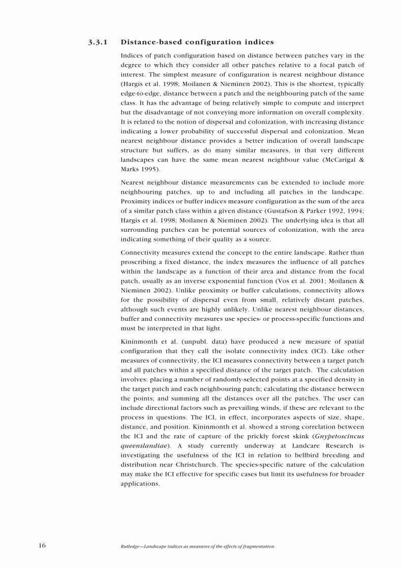
3.3.1 Distance-based configuration indices
Indices of patch configuration based on distance between patches vary in the
degree to which they consider all other patches relative to a focal patch of
interest. The simplest measure of configuration is nearest neighbour distance
(Hargis et al. 1998; Moilanen & Nieminen 2002). This is the shortest, typically
edge-to-edge, distance between a patch and the neighbouring patch of the same
class. It has the advantage of being relatively simple to compute and interpret
but the disadvantage of not conveying more information on overall complexity.
It is related to the notion of dispersal and colonization, with increasing distance
indicating a lower probability of successful dispersal and colonization. Mean
nearest neighbour distance provides a better indication of overall landscape
structure but suffers, as do many similar measures, in that very different
landscapes can have the same mean nearest neighbour value (McCarigal &
Marks 1995).
Nearest neighbour distance measurements can be extended to include more
neighbouring patches, up to and including all patches in the landscape.
Proximity indices or buffer indices measure configuration as the sum of the area
of a similar patch class within a given distance (Gustafson & Parker 1992, 1994;
Hargis et al. 1998; Moilanen & Nieminen 2002). The underlying idea is that all
surrounding patches can be potential sources of colonization, with the area
indicating something of their quality as a source.
Connectivity measures extend the concept to the entire landscape. Rather than
proscribing a fixed distance, the index measures the influence of all patches
within the landscape as a function of their area and distance from the focal
patch, usually as an inverse exponential function (Vos et al. 2001; Moilanen &
Nieminen 2002). Unlike proximity or buffer calculations, connectivity allows
for the possibility of dispersal even from small, relatively distant patches,
although such events are highly unlikely. Unlike nearest neighbour distances,
buffer and connectivity measures use species- or process-specific functions and
must be interpreted in that light.
Kininmonth et al. (unpubl. data) have produced a new measure of spatial
configuration that they call the isolate connectivity index (ICI). Like other
measures of connectivity, the ICI measures connectivity between a target patch
and all patches within a specified distance of the target patch. The calculation
involves: placing a number of randomly-selected points at a specified density in
the target patch and each neighbouring patch; calculating the distance between
the points; and summing all the distances over all the patches. The user can
include directional factors such as prevailing winds, if these are relevant to the
process in questions. The ICI, in effect, incorporates aspects of size, shape,
distance, and position. Kininmonth et al. showed a strong correlation between
the ICI and the rate of capture of the prickly forest skink (Gnypetoscincus
queenslandiae). A study currently underway at Landcare Research is
investigating the usefulness of the ICI in relation to bellbird breeding and
distribution near Christchurch. The species-specific nature of the calculation
may make the ICI effective for specific cases but limit its usefulness for broader
applications.

17DOC Science Internal Series 98
3.3.2 Pattern-based configuration indices
Pattern-based indices of configuration attempt to provide a measure of the
overall complexity of the landscape in question. Unlike distance measures, they
do not have a patch focus and are calculated using the entire landscape.
The most widely-used and often-cited measurement of spatial pattern is
contagion (O�Neill, Krummel et al. 1988; Li & Reynolds 1993). Contagion
measures the degree of adjacency between cells on a raster landscape. Measures
vary from near 0 to 100. High values indicate a high degree of adjacency
between cells of the same class (clumped). Low values indicate relatively
similar probabilities of adjacency among classes (random or dispersed). One
problem with contagion is that results can vary depending on the method used
to calculate frequencies of adjacency between cell types (Riitters et al. 1996).
FRAGSTATS (McCarigal & Marks 1995) provides an interspersion/juxtaposition
index that measures adjacency of patches and not just pixels. This index also
varies from 0 to 100 but has the reverse interpretation from contagion. Low
values indicate low levels of interspersion (clumped) while high values indicate
high levels of interspersion (random or dispersed).
Frohn (1998) proposed an alternative to contagion called patch per unit area.
He criticized the contagion index because it can vary depending on the spatial
resolution, the number of classes, and even rotation of an image. He also
provided examples where the contagion index gave counterintuitive results,
i.e. low values for clumped landscapes and high values for random landscapes.
In contrast, patch per unit area remains invariant under scale changes because it
includes a factor that scales with the unit of resolution. It also appears to better
quantify the level of aggregation within a map. Despite these advances, patch
per unit area does not appear to be widely used.
Another measure similar to contagion is patch cohesion (Schumaker 1996).
Patch cohesion measures the degree of aggregation or �connectedness� of
patches and correlates well with dispersal success under a variety of conditions.
In that sense, it is related to contagion but also has indirect connections to
distance-based measures of patch configuration. Patch cohesion shows promise
because it appears to correlate well with a variety of models of dispersal
success. However, the definition of a patch will be different for each species;
thus patch cohesion will be different for each species, making its utility for
broad-scale conservation planning questionable.
Two indices have been proposed recently as alternatives to contagion:
aggregation index and degree of division (He et al. 2000; Jaeger 2000).
Aggregation index measures the degree of aggregation of a particular patch
class on the landscape by comparing the number of shared edges with the total
possible number of shared edges. The level of aggregation can vary from 0 =
completely disaggregated with no shared edges, to 1 = maximum number of
shared edges and completely aggregated. Summing the index values weighted
by proportion of area for all classes provides a measure of landscape
aggregation. Aggregation index varies with varying spatial resolution, but the
index value for individual classes will not be affected by changes in the other
classes. However, it suffers from the same drawback as contagion, in that
different spatial patterns can produce the same value of index.
18 Rutledge�Landscape indices as measures of the effects of fragmentation
Unlike the aggregation index, the degree of division index (Jaeger 2000) is
defined as the probability that two randomly selected locations do not occur
within the same patch in the landscape. As a result, this index relates more to
interspersion/juxtaposition than contagion. The index is ecologically motivated
by the question of how likely it is that two organisms will �find� each other or, in
other words, occur within the same patch. As with the splitting index and
effective mesh size (Section 3.1), the degree of division index has a number of
attractive mathematical features that may make it more useful than other
indices. However, the underlying rationale of random placement of organisms
deserves more thought as the location of an organism in the landscape is not a
completely random process.
Lacunarity (from the Latin, lacuna = gap), differs from contagion or similar
measures, by measuring the degree of gaps between features of interest on a
map (Plotnick et al. 1993). Measuring lacunarity involves sliding a window of a
fixed size across a landscape and counting the number of cells of interest within
the box. Landscapes with a higher degree of aggregation will have larger
intervening gaps and consequently a higher degree of lacunarity. Because the
measure depends on window size, a more illuminating analysis involves
plotting lacunarity versus box size to examine whether gap size varies with
scale. Despite its relatively early introduction to the landscape ecology
literature, lacunarity analysis has received little treatment in it. One recent
study suggests that lacunarity correlates better with dispersal success on
landscapes with a low proportion (< 10%) of habitat than measures such as
number of patches or landscape connectivity (With & King 1999).
4. Landscape indices andecosystem fragmentation:what do we know?
What can the landscape indices described in Section 3 tell us about the effects
of fragmentation and can we use those indices to help manage remaining
patches of ecosystems more effectively? One way to answer this question is to
examine the development of landscape indices over time to determine what
insights they have provided regarding different ecological processes.
The development of fragmentation indices mostly parallels the development of
landscape ecology. Landscape ecology is still best summarized by the title of
Turner�s (1989) seminal review: �Landscape Ecology: The Effect of Pattern on
Process.� The field developed in response to the increasing need to understand
how species and ecosystems have fared as the extent of human activities
expands across the globe (Urban et al. 1987; Turner 1989; Hobbs 1995).
Initially landscape ecology adopted an Island Biogeographic viewpoint
(MacArthur & Wilson 1967) and equated remaining patches of natural
ecosystems with islands and the surrounding areas of man-made ecosystems
19DOC Science Internal Series 98
with oceans. Over the years the viewpoint has evolved, and spatial
heterogeneity, which is not well approximated by a mainland-island model,
became important (Gustafson & Gardner 1996). Considerations of scale and
ecological hierarchies have also received increasing amounts of attention to the
point that scale is now a pervasive issue throughout all branches of ecology
(Haila 2002; Wu & Qi 2000).
Early efforts focused on developing indices to describe landscape pattern and
understand the effect of varying basic landscape attributes on those indices.
The basic attributes studied included the number of patch classes, the spatial
extent of the landscape, the scale (or grain) of the study (Turner et al. 1989;
Turner 1990) and the proportion of a patch class within the landscape
(Gustafson & Parker 1992). Most studies represented landscapes as grids (or
raster maps) because grids corresponded directly to the remote-sensing imagery
that was becoming widely available (O�Neill, Krummel et al. 1988). These
studies indicated that the scale (grain and extent) of study and proportion of
patch classes affects many landscape indices, making comparisons among
landscapes studied under different conditions problematic.
A significant milestone in the development and use of landscape indices
occurred in 1994 when FRAGSTATS (McCarigal & Marks 1995) and r.le (Baker &
Cai 1992) became available. FRAGSTATS, r.le, and the follow-on program Patch
Analyst (Rempel et al. 1999) brought landscape pattern analysis to the masses.
They also brought a plethora of landscape metrics to characterise attributes of
individual patches, patch classes, or entire landscapes. The utility and
usefulness of these programs are evidenced by their continued use. In fact, a
new version of FRAGSTATS has just been developed and released (McCarigal et
al. 2002) that includes several recently-proposed landscape metrics.
The following year, Riitters et al. (1995) published an analysis of landscape
indices that suggested using fewer, not more, indices. They analysed 55
landscape indices and found high levels of correlation among them. They then
selected a subset of 26 indices, chosen to reduce correlations, and showed that a
set of six indices could represent most of the variation in landscape structure.
Cain et al. (1997) then compared a set of landscape metrics for a large set of maps
for two regions of the United States. Except for one factor related to contagion,
the order of importance of the remaining factors varied for different maps.
Following the Riitters et al. (1995) paper, efforts went into reviewing and
evaluating the current set of landscape indices and their linkages to ecological
processes, particularly dispersal. For example, Hargis et al. (1998) examined the
behaviour of landscape metrics in relation to spatial arrangement while
controlling for patch size and patch shape. The landscape metrics were highly
correlated and were, �relatively insensitive to variations in the spatial
arrangement of patches on the landscape.� Further development of ecological
indices has had a much stronger basis in ecological theory, again with a strong
emphasis on the relationship between species dispersal and the spatial
configuration of the patch network.
Finally, a series of papers have recently been published that paint a highly
complex picture of fragmentation and call into question the efficacy of using
simple landscape indices as indicators of ecological conditions. These papers
modeled species persistence or movement on landscapes with differing levels

20 Rutledge�Landscape indices as measures of the effects of fragmentation
of habitat amount, fragmentation, and/or arrangement. The general conclusion
is that the dominant factor in determining species persistence is the total
amount of habitat (Fahrig 2002; Flather & Bevers 2002). Species persist until a
particular amount of habitat is reached, regardless of arrangement, and then
exhibit relatively quick declines in population size or persistence, which are
termed �threshold effects� (Fig. 1). However, threshold values varied
considerably depending upon any number of life history parameters of the
species in question (Fahrig 2001; With & King 2001). Further, empirical studies
demonstrated that the effects of fragmentation vary widely among species
(Harrison & Bruna 1999; Debinski & Holt 2000; Tscharntke et al. 2002).
5. Conclusions
The development of landscape indices can be divided into three periods:
proliferation, re-evaluation, and redirection. From the mid-1980s to the mid-
1990s, the number of landscape indices grew as researchers began to emphasize
the importance of understanding how and to what degree the patterns of
fragmented natural ecosystems affected ecological processes. In response, they
created a large number of indices to discern and compare different landscape
patterns. From the mid-1990s to approximately 2000, the behaviour and utility
of many indices were re-evaluated. Many indices were highly correlated or
showed highly variable relationships with different ecological processes. The
few, new indices developed during this period attempted to overcome
deficiencies in previous indices. This period also included much work on
understanding the ecological effects of pattern as distinct from quantification of
pattern. From 2000 to the present, the emphasis has shifted towards the
Figure 1. Example of thethreshold effect. The
probability that a specieswill persist in the
landscape remains highwhen total habitat area
comprises at least 40% oftotal landscape area. Whentotal habitat area decreases
to less than 40% (dashedline) of total landscapearea, the probability of
persistence begins todecline rapidly.
Total habitat area (% of total landscape area)
Pro
babi
lity
of p
ersi
sten
ce
0 20 40 60 80 100
1
0

21DOC Science Internal Series 98
development of more ecologically-motivated indices as well as the
consideration of pattern as part of the ecological process itself.
In summary, landscape indices: vary with varying landscape attributes (grain,
extent, number of classes, etc.); correlate highly with one another and often
provide redundant information�which is not surprising, given they derive from
a rather small set of possible attributes (area, border or edge length, distance) that
one can measure; and relate differently to different processes, i.e. an index may
prove useful for one process and not another. These results should not be
surprising. The fragmentation of an ecosystem is a complex process that acts on a
complex system and results in a wide arrangement of spatial patterns.
Given their inability to characterise consistently the effect of pattern on process
for simple processes, landscape indices will probably have even less usefulness
for more complex ecological relationships such as trophic interactions.
Theoretical and empirical studies typically focus on a single aspect of one (or at
most a few) species. With respect to fragmentation, the most studied aspect�
probably rightly so�has been dispersal among patches. It appears that the
performance of landscape indices in relation to species interactions has
received less attention.
In light of these findings, how useful are landscape indices? First, they have a
descriptive value in comparing spatial patterns between/among landscapes,
much as general descriptions of �habitat� help paint a picture of where species
live. Second, some indices may relate consistently to specific ecological
processes, such as the relationship between the ICI and skink capture rates
(Kininmonth et al., unpubl. data) or between the patch cohesion index
(Schumaker 1996) and dispersal success. In those cases, using a landscape index
to indicate condition may be appropriate. However, as Gustafson (1998) notes,
�Indices may be used as correlations, but ultimately what really matters is the
process of interest.�
Research should emphasize gaining knowledge and developing techniques that
directly characterise ecological processes and conditions. This approach has
the advantage that it requires unambiguous definition of the process,
measurement units, and scale of interest. Consider, for example,
metapopulation ecology, which seeks to understand the dynamics of a network
of populations that are spread across a heterogeneous landscape and are
connected to one another by dispersal (Hanski & Gilpin 1991; Hanski 1999).
Metapopulation ecology overlaps significantly with landscape ecology in terms
of conceptual domain. However, they take different approaches to the issue of
fragmentation. (For an interesting exchange related to this difference, see
Tischendorf & Fahrig 2000a; Moilanen & Hanski 2001; Tischendorf & Fahrig
2001.) As previously discussed, landscape ecology often measures pattern first
and then determines whether the measurement relates to an actual process.
Conversely, metapopulation ecology considers pattern as part of process, for
example that recolonization rates are inversely proportional to distance from
source. The latter approach relates directly to real-world concerns over species
persistence. Disagreements may arise about the manner in which pattern is
incorporated into process, but those disagreements will stimulate further
research on ecological processes and how to measure them realistically.

22 Rutledge�Landscape indices as measures of the effects of fragmentation
6. Future research
If the research focus shifts towards directly characterising ecological conditions
and processes, the question then becomes: given the multitude of ecological
processes and patterns operating across a variety of scales, what is the best way
to proceed? In this regard, the 15 to 20 years of research on landscape indices
may offer some guidance. Below are five important areas of investigation
suggested by that body of research. The five areas represent a starting point for
further investigations but certainly do not address all aspects of the study of
fragmentation.
1. What proportion of total area is required to sustain a particular process or
species? What total area (extent) is needed to make that decision?
In general �bigger is better� or more area is preferable to less area (e.g. Bender et
al. 1998; Debinski & Holt 2000). A potential �threshold effect� (Fig. 1) may exist
for many species if the amount of habitat (however defined) falls below a
particular proportion of the landscape (Fahrig 2001; Fahrig 2002). What are
those proportions for different species? How large (what extent of) an area
must be measured to calculate the proportion? Does the threshold effect apply
broadly to species and processes or only to the process of dispersal? Such
information could contribute directly to landscape planning. For example,
Lambeck (1997) proposed using focal species to establish minimum areas for
conservation. Focal species are those with the largest area requirements, such
as birds that require forest patches of a particular size to breed.
2. As the total area decreases, what aspects of fragmentation (composition,
shape, configuration) become important to maintain the species or process of
interest? Does that knowledge contribute to offsetting the effects of
fragmentation?
A decrease in total area affects many processes, including species viability,
dispersal, threat of invasion, etc. (Saunders et al.1991; Debinski & Holt 2000;
Olff & Ritchie 2002). As the total area decreases, the spatial pattern of the
remaining areas becomes more important. In these cases, are there discernible
relationships between spatial pattern and the magnitude and direction of
change to the species or process in question? Can spatial pattern be
manipulated to compensate for lost area?
3. At what scale does a process operate? Given a known process operating at a
particular scale, what can be done to prevent further fragmentation or restore
connectivity?
Different processes operate at different scales (With 1994). Consider two
identical forest patches: one isolated by several kilometres from any other
forest patch and one contained within a network of forest patches. Over time
the trajectories of change of the patches will differ, owing to the spatial pattern
of the surrounding landscape. What processes do the two fragments share and
what processes are different? For the isolated fragment, which processes
become �disconnected?� What are the consequences of disconnection, e.g. no
recolonization by native species versus no invasion by exotic weeds, both of
which are unable to cross pasture? Graph theory, not previously discussed in
this review, may be able to answer such questions (Cantwell & Forman 1993;

23DOC Science Internal Series 98
Keitt et al. 1997; Urban & Keitt 2001). Graph theory represents features as a
network of nodes and connections. Using information on connectivity,
networks can be analysed to show when disconnections occur because nodes
are lost or, when connections occur if nodes are added. This has direct
applications for reserve design and restoration. Also, the approach is appealing
because its results can be visually depicted.
4. How does spatial pattern affect the distribution and abundance of exotic
species and the control of those species?
New Zealand has many exotic species subject to varying levels of management
control. However, until very recently, little work had been done to understand
the relationship between spatial pattern and the distribution, abundance, and
influence of these species. Several questions can be asked. At what scales do
these species operate? What effect does the spatial pattern of control have on
the target species and native species/ecosystems? Can controls be patterned to
increase their overall effectiveness? Can graph theory (see, Question 3) or
similar methods contribute to more effective control?
5. How does ecosystem pattern change as the scale of information changes? How
do those changes affect models of ecological processes and their results? How
do we interpret different levels of information relative to distribution of
resources needed by different species?
The scale of information receives relatively little attention relative to spatial and
temporal scale. For example, the New Zealand Land Cover Database (Ministry
for the Environment 1997) has a class termed �indigenous forest.� Indigenous
forest spans a broad range of conditions. At the opposite extreme, the �urban�
class may actually contain resources used by many native species. How well do
we understand the relationship between land cover/land use, which is often
what is measured, and various ecological processes? Can more detailed
information lead to improved biodiversity in man-made ecosystems?
These questions represent some of the most important issues regarding the
effects of spatial pattern and ecosystem fragmentation. This paper demonstrates
that landscape indices have provided some insights into these processes but for
many reasons do not adequately indicate the effect of pattern on process. At
best, such indices provide a measure of ecosystem pattern that can be used in a
descriptive sense to compare different landscapes. A better strategy is to
conduct research that develops the knowledge and techniques needed to
incorporate the effects of ecosystem pattern directly into models of process.
Models of process, such as those offered by metapopulation ecology or graph
theory, provide information on ecosystem condition given different spatial
patterns. The information gained can then be used to evaluate and decide
between different management actions, resulting in more effective use of
conservation resources and larger gains in conservation outcomes.

24 Rutledge�Landscape indices as measures of the effects of fragmentation
7. Acknowledgements
The author would like to thank Bruce Burns, Jake Overton, and Theo Stephens
for many helpful comments on draft versions of the report. The author also
would like to thank Rochelle Russell for report formatting, Anne Austin for
editorial oversight, and Pam Byrne at the Landcare Research library for timely
delivery of the many articles needed for this review. The Department of
Conservation (investigation no 3628) funded this review.
8. References
Baker, W.L.; Cai, Y. 1992: The r.le programs for multiscale analysis of landscape structure using the
GRASS geographical information system. Landscape Ecology 7: 291�302.
Bender, D.J.; Contretras, T.A.; Fahrig, L. 1998: Habitat loss and population decline: a meta-analysis of
the patch size effect. Ecology 79: 517�533.
Benson, B.J.; MacKenzie, M.D. 1995: Effects of sensor spatial resolution on landscape structure
parameters. Landscape Ecology 10: 113�120.
Berry, L. 2001: Edge effects on the distribution and abundance of birds in a southern Victorian forest.
Wildlife Research 28: 239�245.
Bregt, A.K.; Wopereis, M.C.S. 1990: Comparison of complexity measures for choropleth maps. The
Cartographic Journal 27: 85�91.
Cain, D.H.; Riitters, K.; Orvis, K. 1997: A multi-scale analysis of landscape statistics. Landscape
Ecology 12: 199-212.
Cantwell, M.D.; Forman, R.T.T. 1993: Landscape graphs: ecological modeling with graph theory to
detect configurations common to diverse landscapes. Landscape Ecology 8: 239�255.
Debinski, D.M.; Holt, R.D. 2000: A survey and overview of habitat fragmentation experiments.
Conservation Biology 14: 342�355.
Didham, R.K. 1998: Altered leaf-litter decomposition rates in tropical forest fragments. Oecologia
116: 397�406.
Fahrig, L. 2001: How much habitat is enough? Biological Conservation 100: 65�74.
Fahrig, L. 2002: Effect of habitat fragmentation on the extinction threshold: a synthesis. Ecological
Applications 12: 346�353.
Flather, C.H.; Bevers, M. 2002: Patchy reaction-diffusion and population abundance: the relative
importance of habitat amount and arrangement. The American Naturalist 159: 40�56.
Forman, R.T.T. 1995: Land mosaics: the ecology of landscapes and regions. Cambridge University
Press, Cambridge, UK. 632 p.
Frohn, R.C. 1998: Remote sensing for landscape ecology: new metric indicators for monitoring,
modeling, and assessment of ecosystems. Lewis Publishers, Boca Raton, Florida. 99 p.
Gustafson, E.J. 1998: Quantifying landscape spatial pattern: what is the state of the art? Ecosystems 1:
143�156.
Gustafson, E.J.; Gardner, R.H. 1996: The effect of landscape heterogeneity on the probability of
patch colonization. Ecology 77: 94�107.
25DOC Science Internal Series 98
Gustafson, E.J.; Parker, G.R. 1992: Relationships between landcover proportion and indices of
landscape pattern. Landscape Ecology 7: 101�110.
Gustafson, E.J.; Parker, G.R. 1994: Using an index of habitat patch proximity for landscape design.
Landscape and Urban Planning 29: 117�130.
Haila, Y. 2002: A conceptual genealogy of fragmentation research: from island biogeography to
landscape ecology. Ecological Applications 12: 321�334.
Hall, L.S.; Krausman, P.R.; Morrison, M.L. 1997: The habitat concept and a plea for standard
terminology. Wildlife Society Bulletin 25: 173�182.
Hanski, I. 1999: Metapopulation ecology. Oxford series in ecology and evolution. Oxford University
Press, Oxford. 313 p.
Hanski, I.; Gilpin, M. 1991: Metapopulation dynamics: brief history and conceptual domain.
Biological Journal of the Linnean Society 42: 3�16.
Hanski, I.; Simberloff D. 1997: The metapopulation approach: its history, conceptual domain, and
application to conservation. Pp. 5�26 in Hanski, I.A.; Gilpin, M.E. (Eds): Metapopulation
biology: ecology, genetics, and evolution. Academic Press Inc., San Diego.
Hargis, C.D.; Bissonette, J.A.; David, J.L. 1997: Understanding measures of landscape pattern. Pp.
231-261 in Bissonette, J.A. (Ed.): Wildlife and landscape ecology: effects of pattern and scale.
Springer-Verlag, New York.
Hargis, C.D.; Bissonette, J.A.; David, J.L. 1998: The behavior of landscape metrics commonly used in
the study of habitat fragmentation. Landscape Ecology 13: 167�186.
Harrison, S.; Bruna, E. 1999: Habitat fragmentation and large-scale conservation: what do we know
for sure? Ecography 22: 225�232.
He, H.S.; DeZonia, B.E.; Mladennoff, D.J. 2000: An aggregation index (AI) to quanitfy spatial patterns
of landscapes. Landscape Ecology 15: 591�601.
Hobbs, R.J. 1995: Landscape ecology. Pp. 417�428 in Nierenberg, W.A. (Ed.): Encyclopedia of
environmental biology, vol. 2. Academic Press, Inc., San Diego.
Huxel, G.R.; Hastings, A. 1999: Habitat loss, fragmentation, and restoration. Restoration Ecology 7:
309�315.
Jaeger, J.A.G. 2000: Landscape division, splitting index, and effective mesh size: new measures of
landscape fragmentation. Landscape Ecology 15: 115�130.
Keitt, T.H.; Urban, D.L.; Milne, B.T. 1997: Detecting critical scales in fragmented landscapes.
Conservation Ecology [online] 1:4.
Krummel, J.R.; Gardner, R.H.; Sugihara, G.; O�Neill, R.V.; Coleman, P.R. 1987: Landscape patterns in
a disturbed environment. Oikos 48: 321�324.
Lambeck, R.J. 1997: Focal species: a multi-species umbrella for nature conservation. Conservation
Biology 11: 849�856.
Leathwick, J.; Wilson, G.; Rutledge, D.; Wardle, P.; Morgan, F.; Johnston, K.; MacLeod, M.;
Kirkpatrick, R. In press: Land environments of New Zealand. David Bateman Ltd, Auckland,
NZ.
Li, H.; Reynolds, J.F. 1993: A new contagion index to quantify spatial patterns of landscapes.
Landscape Ecology 8: 153�162.
MacArthur, R.; Wilson, E.O. 1967: The theory of island biogeography. Princeton University Press,
Princeton, New Jersey. 203 p.
MacNally, R.; Brown, G.W. 2001: Reptiles and habitat fragmentation in the box-ironbark forests of
central Victoria: predictions, compositional change, and faunal nestedness. Oecologia 128:
116�125.
MacNally, R.; Horrocks, G. 2002: Relative influences of patch, landscape, and historical factors on
birds in an Australian fragmented landscape. Journal of Biogeography 29: 1�16.
26 Rutledge�Landscape indices as measures of the effects of fragmentation
McCarigal, K.; Cushman, S.A.; Neel, M.C.; Ene, E. 2002: FRAGSTATS: Spatial pattern analysis
program for categorical maps, version 3.0. University of Massachusetts, Amherst,
Massachusetts.
McCarigal, K.; Marks, B.J. 1995: FRAGSTATS: spatial pattern analysis program for quantifying
landscape structure. US Department of Agriculture, Forest Service, General Technical
Report PNW-GTR-351.
Milne, B.T. 1991: Lessons from applying fractal models to landscape patterns. Pp. 199�235 in Turner,
M.G.; Gardner, R.H. (Eds): Quantitative methods in landscape ecology. Springer-Verlag, New
York.
Ministry for the Environment 1997: New Zealand land cover database. New Zealand Ministry for the
Environment. http://www.environment.govt.nz/indicators/land/landcover/
Moilanen, A.; Hanski, I. 2001: On the use of connectivity measures in spatial ecology. Oikos 95: 147�
151.
Moilanen, A.; Nieminen, M. 2002: Simple connectivity measures in spatial ecology. Ecology 83:
1131�1145.
Morrison, M.L.; Marcot, B.G.; Mannan, R.W. 1992: Wildlife-habitat relationships: concepts and
applications. University of Wisconsin Press, Madison, Wisconsin. 343 p.
O�Neill, R.V.; Krummel, J.R.; Gardner, R.H.; Sugihara, G.; Jackson, B.; DeAngelis, D.L.; Milne, B.T.;
Turner, M.G.; Zygmunt, B.; Christensen, S.W.; Dale, V.H.; Graham, R.L. 1988: Indices of
landscape pattern. Landscape Ecology 1: 153�162.
O�Neill, R.V.; Milne, B.T.; Turner, M.G.; Gardner, R.H. 1988: Resource utilization scales and
landscape pattern. Landscape Ecology 2: 63�69.
Olff, H.; Ritchie, M.E. 2002: Fragmented nature: consequences of biodiversity. Landscape and
Urban Planning 58: 83�92.
Patton, D.R. 1975: A diversity index for quantifying habitat �edge�. Wildlife Society Bulletin 3: 171�
173.
Pearson, S.M.; Turner, M.G.; Gardner, R.H.; O�Neill, R.V. 1996: An organism-based perspective of
habitat fragmentation. Pp. 77-95 in Szaro, R.C.; Johnson, D.W. (Eds): Biodiversity in
managed landscapes: theory and practice. Oxford University Press, New York.
Plotnick, R.E.; Gardner, R.H.; O�Neill, R.V. 1993: Lacunarity indices as measures of landscape
texture. Landscape Ecology 8: 201�211.
Pulliam, H.R. 1988: Sources, sinks, and population regulation. American Naturalist 132: 652�661.
Rempel, R.S.; Carr, A.; Elkie, P. 1999: Patch analyst and patch analyst (grid) function, reference
version 2.0. Ontario Ministry of Natural Resources, Lakehead University, Centre for
Northern Forest Ecosystem Research, Thunder Bay, Ontario, Canada.
Riitters, K.H.; O�Neill, R.V.; Hunsaker, C.T.; Wickam, J.D.; Yankee, D.H.; Timmins, S.P.; Jones, K.B.;
Jackson, B.L. 1995: A factor analysis of landscape pattern and structure metrics. Landscape
Ecology 10: 23�29.
Riitters, K.H.; O�Neill, R.V.; Wickam, J.D.; Jones, K.B. 1996: A note on contagion indices for
landscape analysis. Landscape Ecology 11: 197�202.
Saunders, D.A.; Hobbs, R.J.; Margules, C.R. 1991: Biological consequences of ecosystem
fragmentation: a review. Conservation Biology 5: 18�32.
Saura, S.; Martinez-Millan, J. 2001: Sensitivity of landscape pattern metrics to map spatial extent.
Photogrammetric Engineering and Remote Sensing 67: 1027�1036.
Schumaker, N.H. 1996: Using landscape indices to predict habitat connectivity. Ecology 77: 1210�
1225.
Sumner, J.; Moritz, C.; Shine, R. 1999: Shrinking forest shrinks skinks: morphological change in
response to rainforest fragmentation in the prickly forest skink (Gnypetoscincus
queenslandia). Biological Conservation 91: 159�167.

27DOC Science Internal Series 98
Tischendorf, L. 2001: Can landscape indices predict ecological processes consistently? Landscape
Ecology 16: 235�254.
Tischendorf, L.; Fahrig, L. 2000a: How should we measure landscape connectivity? Landscape
Ecology 15: 633�641.
Tischendorf, L.; Fahrig, L. 2000b: On the usage and measurement of landscape connectivity. Oikos
90: 7�19.
Tischendorf, L.; Fahrig, L. 2001: On the use of connectivity measures in spatial ecology: a reply.
Oikos 95: 152�154.
Tscharntke, T.; Steffan-Dewenter, I.; Kruess, A.; Thies, C. 2002: Contribution of small habitat
fragments to conservation of insect communities of grassland-cropland landscapes.
Ecological Applications 12: 354�363.
Turner, M.G. 1989: Landscape ecology: the effect of pattern on process. Annual Review of Ecology
and Systematics 20: 179�197.
Turner, M.G. 1990: Spatial and temporal analysis of landscape patterns. Landscape Ecology 4: 21�
30.
Turner, M.G.; O�Neill, R.V.; Gardner, R.H.; Milne, B.T. 1989: Effects of changing spatial scale on the
analysis of landscape pattern. Landscape Ecology 3: 153�162.
Urban, D.; Keitt, T. 2001: Landscape connectivity: a graph-theoretic perspective. Ecology 82: 1205�
1218.
Urban, D.L.; O�Neill, R.V.; Shugart, H.H. 1987: Landscape ecology: a hierarchical perspective can
help scientists understand spatial patterns. Bioscience 37: 119�127.
Verboom, J. Schotman, A.; Opdam, P.; Metz, J.A.J. 1991. European nuthatch metapopulations in a
fragmented agricultural landscape. Oikos 61: 149�156.
Vos, C.C.; Verboom, J.; Opdam, P.F.M.; Ter Braak, C.J.F. 2001: Toward ecologically scaled
landscape indices. The American Naturalist 183: 24�41.
With, K.A. 1994: Using fractal analysis to assess how species perceive landscape structure.
Landscape Ecology 9: 25�36.
With, K.A.; King, A.W. 1999: Dispersal success on fractal landscapes: a consequence of lacunarity
thresholds. Landscape Ecology 14: 73�82.
With, K.A.; King, A.W. 2001: Analysis of landscape sources and sinks: the effect of spatial pattern on
avian demography. Biological Conservation 100: 75�88.
Wu, J.; Qi, Y. 2000: Dealing with scale in landscape analysis: an overview. Geographic Information
Sciences 6: 1�5.