Landmark Recognition Using Machine Learning Andrew Crudge, Will Thomas and Kaiyuan Zhu

Introduction As smartphones and mobile data become more prevalent in modern society, the

possibilities for them to interact with the physical world also grow exponentially. Technologies such as Oculus Rift and Google Glass are attempting to bridge the gap between the virtual and the physical, and as enhancements in computer speed and image processing are made, the concept of Augmented Reality (AR) becomes more tangible.

However, one difficulty with AR is the sheer complexity of image processing and feature recognition. A successful AR system must be able to distinguish among a large number of landmarks and should be able to adapt to the existence of new landmarks. Because of the adaptability requirement, AR algorithms naturally lend themselves to using machine learning. As such, the focus of this project is to develop, refine and document a machine learning algorithm that can distinguish landmarks from images using a database of known landmarks.

Data and Preprocessing The input data consists of 193 images of various buildings collected from Google

Images. The training data to be put into the SVM consists of a vector that contains all the labels, and a matrix whose rows are the examples and whose columns are the features. To make each example the same feature dimension, the image is cropped to an aspect ratio of 5:2. This specific aspect ratio is chosen for all images because most landmarks are skyscrapers that requires more height than width to capture the main features. Then, the images are converted into grayscale because the HOG descriptor looks for differences in gradient intensity, regardless of which colors are used. Lastly, the images are shrunk to 250x100 pixels, preserving the original aspect ratio, so that each image will generate an identical feature size.

Feature Extraction To extract features from the images, Histogram of Oriented Gradients (HOG) was used.

HOG descriptors are useful for object detection because they analyze gradient orientation in localized regions of an image. The image is divided into small regions called cells. Within each cell, the gradient directions of the pixels are analyzed and formed into a 1-D histogram [1]. These histograms are then combined to generate the features of the algorithm.

HOG descriptors were chosen to extract the features from the input images because they are well-suited for object detection. By analyzing the gradient directions of the pixels in the image, the descriptor is able to differentiate the edge of a building from the background.

The HOG descriptor also possesses several other useful properties for object detection. In particular, it is invariant to shadows or changes in illumination. This is achieved by combining neighboring cells into a larger region called a block and computing a measure of the intensity of the block. This intensity is then used to normalize the cells within the block [1]. One drawback of the HOG tool is that it is not invariant to changes in orientation. This will not be a big issue in the preliminary application as long as the buildings in the image are roughly upright.

The effectiveness of the HOG depends on the cell size chosen for the algorithm. Indeed, varying the cell size changes the number of features generated for each example. A smaller cell

1

more information about the image. However, smaller cell size also increases the running time of the algorithm since the larger feature vectors take more time to process. The effects of the cell size of HOG on the accuracy of the algorithm can be seen in Figure 1.

Figure 1: Accuracy of the SVM classifier as a function of the cell size of the HOG descriptor

As cell size increases, the test accuracy of the algorithm decreases. The algorithm

achieves the highest accuracy of 95% with a cell size of 5x5. However, the accuracy drops below 85% once the cell size grows to 25x25. After balancing the algorithm’s runtime and performance, a cell size of 17x17 was selected. Another feature extraction algorithm, Segmentation Based Fractal Analysis (SFTA), was considered. However, this method generates feature vectors much slower and with a maximum accuracy of 70% - much poorer than HOG.

Models A Support Vector Machine (SVM) was selected as the primary machine learning classifier

for this application. This model was chosen because the algorithm is very efficient when dealing with high dimensional feature spaces. Additionally, SVM usually has the best performance among the other “off-the-shelf” supervised learning algorithm, and is very popular in many industrial applications. In the application, feature vectors are produced through HOG descriptor with 17x17 cell size, and the resulting feature dimension is above 1500.

Results and Discussions The four classifiers were compared by being run on a dataset of 100 images. The

dataset was split into a training set consisting of 80 images and a test set consisting of the remaining 20 images. To obtain an accurate evaluation of the performance, each classifier was run 20 times. Each time, the dataset was randomly permuted to vary the training and test sets. The average performance of each classifier was then computed over the 20 runs. The results of the experiment can be found in Table 1.

2

Classifier Training Accuracy Test Accuracy

Support Vector Machine 1 0.9200

Discriminant Analysis 1 0.9050

Naïve Bayes Classifier 0.8642 0.8500

Linear Regression 1 0.8000 Table 1: Relative performance of various classifiers

The performance of the classifiers on the test set ranges from 80-92%. Among the four

classifiers, the Support Vector Machine attains the highest average test accuracy. In addition, it runs much faster than the other classifiers. As a result, it was selected for the application.

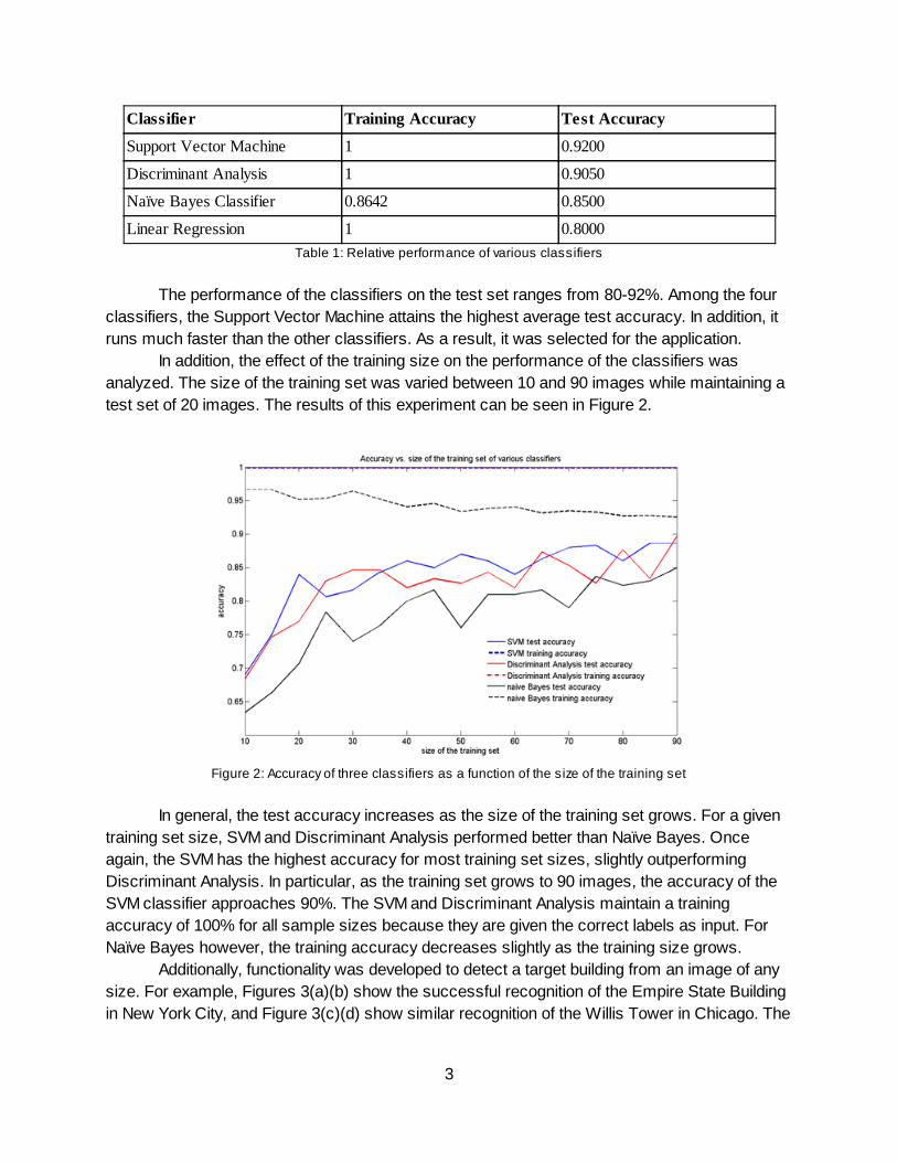
In addition, the effect of the training size on the performance of the classifiers was analyzed. The size of the training set was varied between 10 and 90 images while maintaining a test set of 20 images. The results of this experiment can be seen in Figure 2.

Figure 2: Accuracy of three classifiers as a function of the size of the training set

In general, the test accuracy increases as the size of the training set grows. For a given

training set size, SVM and Discriminant Analysis performed better than Naïve Bayes. Once again, the SVM has the highest accuracy for most training set sizes, slightly outperforming Discriminant Analysis. In particular, as the training set grows to 90 images, the accuracy of the SVM classifier approaches 90%. The SVM and Discriminant Analysis maintain a training accuracy of 100% for all sample sizes because they are given the correct labels as input. For Naïve Bayes however, the training accuracy decreases slightly as the training size grows.

Additionally, functionality was developed to detect a target building from an image of any size. For example, Figures 3(a)(b) show the successful recognition of the Empire State Building in New York City, and Figure 3(c)(d) show similar recognition of the Willis Tower in Chicago. The

3

box in the images shows the algorithm’s guess as to the location of the target building. In both cases, the algorithm is able to correctly identify the target building.

(a)

(b)

(c)

(d)

(e)

(f)

Figure 3: Algorithm Identifies Target Buildings from Image of New York City and Chicago Skylines

4

To detect a target building hidden within a larger image, the image is cropped into

multiple overlapping cells with identical aspect ratios. Features are then extracted from the cells using the HOG descriptor and classified using the SVM algorithm outlined above. For each cell, the classifier outputs a labeling and a confidence. The cell with the largest confidence of being classified as a positive labeling is then deemed the most likely cell to contain the target building. Finally, the algorithm was adapted to analyze images containing multiple target buildings. To handle multiple target buildings in a single image, the problem was divided into multiple, independent binary classification tasks. As before, the image was divided into cells and a labeling and confidence was assigned to each cell using the SVM. If an example has multiple cells that are assigned the same label, the cell with the higher confidence score is assigned the label. Using this method, two target buildings could be detected from one image with an accuracy of 85%. Combining the algorithm of multi-class classification and algorithm of recognizing target building in a large image, the result in Figure 3(e)(f) was produced, in which the algorithm successfully identifies the Empire State Building and the Chrysler Building from an image of the New York City skyline.

Conclusions and Future Work Overall, the results are very encouraging, and they demonstrate that landmarks can be

accurately identified from an image using a basic classification algorithm. An accuracy as high as 90% is attainable using a relatively small sample size.

Furthermore, the time required to process and analyze an image is reasonable. These results suggest that this algorithm could be incorporated into an App to provide real-time feedback as images are taken.

In the future, other feature extraction methods can be looked at that may give better accuracy but require fewer dimensions. An algorithm will also need to be developed that can automatically search and obtain data from a database. The project can ultimately become part of the back-end code for a feature-recognition smartphone app.

References [1] N. Dalal and B. Triggs, "Histograms of oriented gradients for human detection ", CVPR, 2005

5