Land Cover Type Changes Related to

Oil and Natural Gas Drill Sites in a

Selected Area of Williams County, ND

FR 3262/5262 Lab Section 2

By:

Andrew Kernan

Tyler Kaebisch

Introduction:

In recent years, there has been a sharp increase in oil and natural gas production in northwest

North Dakota and many communities are experiencing a ‘boom town’ response. Over the years

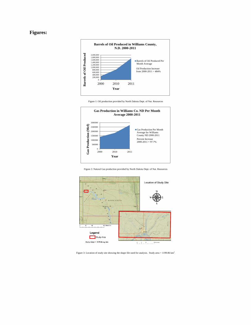
of 2000 to 2011, in Williams County, ND, there has been an increase of oil production by 484%

and an increase of natural gas production by 97.7% (Figure 1 and 2, North Dakota DNR, 2013).

As the communities grow, the land cover types of the communities change. Change in land

cover type from agriculture to residential or from forest to agriculture may occur in these

growing communities. The increase of oil and natural gas production will also show a change

from some previous land cover type to an oil or natural gas drill site which can been seen from

aerial photography as small areas of bare soil. This project will analyze the change in land cover

type from forest and agriculture to bare soil over the period of August 2000 to August 2011

using aerial images acquired by Landsat 5.

Objectives:

In northwestern North Dakota, the town of Williston has experienced an increase in oil and

natural gas production. This study will look specifically at the change in land cover types in an

area within the Little Muddy River Drainage, north of the Missouri River, in Williams County,

North Dakota. The total approximate area of our study site is 1199.86 km2 which can be seen in

Figure 3 in the appendix.

By analyzing images downloaded from Landsat 5 from two separate dates (August 28th, 2000

and August 27th 2011), we expect to see a change in land cover types from cultivated cropland

and forested sites to a land cover type of bare soil where oil and natural gas drill sites are

occurring. This change in land cover type can be used to quantify the increase or decrease of

bare soil in the study site. Data obtained from this project can be used to identify and map oil

and natural gas drill sites and possibly quantify soil erosion and sediment loss. It is important to

monitor land cover changes in order to account for any environmental changes that may occur in

a given site. Changes in water quality, soil erosion and turbidity of local water bodies may be a

result of land cover changes. This project will use remote sensing techniques to analyze land

cover types in our study site. Using remote sensing techniques, we can analyze large areas of

land from multiple dates relatively quickly, compared to gathering data on site. Remote sensing

allows us to view a specific place in time and compare it to a later date, in order to assess the

change in land cover type over time.

Methods:

Downloading Images

Images were acquired from Landsat 5 on two separate dates; one on August 28th, 2000 and one

on August 27th 2011 (a list of all materials used can be found in the appendix). These images

were downloaded from the United States Geological Survey (USGS) Global Visualization

Viewer found at http://glovis.usgs.gov/. Searching in the Lat/Long fields the coordinates

48.1469° N, -103.6175° W and selecting appropriate dates, we were able to obtain images that

contained the town of Williston, ND. By clicking on the ‘Collection’ tab, hovering on ‘Landsat

Archive’ and choosing Landsat 4-5 TM, we were able to select from images gathered by Landsat

5 Thematic Mapper. The Landsat 5 Thematic Mapper (TM) imagery is color infrared and has a

spatial resolution of 30 meters with seven spectral bands. The two dates of imagery selected for

our study were chosen based on limited cloud cover in the area of interest. Originally, we had

wanted to download Landsat 5 TM images from 2012; however, after contacting the USGS Earth

Resources Observation and Science Center’s Technical Services via email, we were informed

that “Landsat 5 TM acquisitions were initially suspended in November of 2011” (USGS, 2013).

We chose to not use images from the Landsat 7 catalog due to the SCL error. After downloading

an image and opening its zip file, the seven spectral bands of the image were stacked together

using ERDAS Imagine software.

Stacking an Image

When an image is downloaded, each spectral band has its own .tif file. All of these .tif files need

to be stacked together to create one .img file for further analysis. In order to stack the layers

together, ERDAS Imagine software is used. In ERDAS Imagine, the Layer Selection and

Stacking window is opened by clicking the ‘Raster’ tab and choosing ‘Spectral’ and then ‘Layer

Stack’. By selecting the Input File browse button and navigating to where the downloaded

image was saved, each spectral band can be selected and ‘added’ one at a time and added to the

layer box. After each of the seven spectral band TIFF files are added to the layer box, an output

file path was specified with a relative name such as ‘stackedImageAug27_2011.img’. The ‘OK’

button was clicked and a layer stack process was started with the result being a new .img file

representing all seven spectral bands stacked together in one image.

Clipping an Image with a newly Created Shapefile

Due to the size of the Landsat imagery (the swath width is 185 km), we clipped our stacked

images so that we could analyze only our study area. In ArcMap, a shape file was created

delineating our study area, seen in Figure 3. This shape was created using the projection

coordinate system of NAD 1983 UTM Zone 13N. In ERDAS Imagine, we loaded one of the

stacked images as a raster into a 2D view and reprojected the image in the UTM GRS 1980 NAD

83 North UTM Zone 13 coordinate system to match the study area shapefile. The study area

shapefile was also loaded into the same 2D view as a vector. A new AOI layer was also created

to copy and clip the image. To clip the Landsat image with the newly created AOI layer, the

‘Create Subset Image’ under ‘Subset and Chip’ was used. The clip process resulted in a new

.img file containing the Landsat 5 TM stacked and reprojected image clipped to the size of our

study area shape file (Figure 4).

Supervised Classification

A supervised classification was performed on the clipped study site Landsat 5 TM images. This

process involved delineating training sites that were used to generate a signature of each class.

One by one, polygons were created using the ‘AOI Drawing tools’ to represent the various land

cover types and each was added to the Signature Class Table and given a descriptive name by

clicking the ‘Add’ icon in the Signature Editor window. Multiple polygons were created for

each class to ensure a strong representation of all pixels in the image. Each polygon was

delineated to represent a homogeneous group of pixels representing a particular class and care

was taken to not include pixels close to the edges of fields. For this project, NAIP imagery was

used as ‘ground truth’ data for the purpose of classifying training areas in the supervised

classification. The NAIP imagery had a 1 meter spatial resolution and helped to define land

cover types in great detail. After a sufficient amount (in our case 85) of training areas were

delineated, the AOI layer and the Signature Editor file were saved in the project folder. In the

Signature Editor, signatures that we knew represented the same class were merged together.

This was done for all signatures and resulted in 15 classes; Forest, Heavy Vegetation, Clear

Water, Turbid Water, Roads, Cropland Type 1, Cropland Type 2, Cropland Type 3, Cropland

Type 4, Cropland Type 5, Cropland Type 6, Cropland Type 7, Cropland Type 8, Cropland Type

9, and Bare Soil. In the ‘Signature Editor’ window, a supervised classification was chosen from

the ‘Classify’ tab and ran with a parametric rule of ‘Maximum Likelihood’. The supervised

classification resulted in a newly created image showing land cover types from the classification

scheme.

Accuracy assessment

An accuracy assessment was performed to show any misclassification of pixels and cover types.

Five stratified random minimum points per class were used for the assessment. The analyst

viewed NAIP imagery for ground truth data to run the assessment. Pixels that were classified

correctly and incorrectly by class were put into an error matrix to report the percent accuracy of

each class. A total percent and a kappa statistic were then produced.

Change Map

Change detection maps of our study area were produced using two methods. The highlighted

change method was used to determine change in brightness values between the clipped Landsat 5

2000 and 2011 images. Increases and decreases in brightness values greater than 17% were

detected by this method. The thematic change method was also used to detect change in our

study area. Thematic change used the supervised classified images of our study area and showed

the amount of direct change from a given class to another.

Results:

The results of the supervised classification for the August 27th, 2011 and August 28th, 2000

images are provided in the appendix in Figure 5. Changes between the two years are noticeable.

The classified land cover types present in the images are; bare soil, crop 0, crop1, crop 2, crop 3,

crop 4, crop 5, crop 6, crop 7, forest, heavy vegetation, moderate vegetation/vegetated cropland

1, moderate vegetation/vegetated cropland 2, road, turbid water and water. The color scheme

associated with each class is listed in the attribute table seen in Figure 6 in the appendix.

The accuracy assessment resulted in an accuracy of 72.27% and a kappa statistic of 68.79%

(Figure 9). The accuracy and kappa percentages were slightly low due to possible inaccuracies

in classification of cover types. The ground truth data used was NAIP imagery within from one

year of the classified images. The analyst classifying the cover types used the NAIP images as

ground truth data and no actual ground truth data was used, therefore; classes may not actually

be correct (i.e. forest cover type may actually be moderate vegetation). Since the accuracy and

the kappa statistic are similar, the assessment of the supervised classification of the images is

somewhat strong.

The results of the highlighted change map and the thematic change map can be viewed in figure

8 in the appendix. With highlighted change, the increase in brightness values correlated well

with areas represented by bare soil. The highlighted change map found in Figure 8 shows a good

representation of areas within the study site that changed to bare soil (shown in green). The

thematic change map (Figure 8) shows the change from one class to another. For the purpose of

this study, the areas of interest were mainly a change from some previous cover type to bare soil.

To show change in forest cover type, the thematic change map also highlights a change in forest

cover to road and forest cover to cropland. This map shows a good representation of change

within our study site. The change in land cover types of forest, cropland, moderate vegetation

and heavy vegetation to bare soil is in detailed in Figure 7. The total hectares changed from

these classes to bare soil was 889.65 hectares, with the highest amount of change taking place in

cropland to bare soil (a change of 525.15 hectares).

Discussion:

The goal of this project was to analyze the change in land cover type from forest and agriculture

to bare soil over time. The areas of bare soil could then be looked at further to map possible drill

sites for oil and natural gas. Throughout the process of classifying the image, multiple issues

arose with the ‘bare soil’ classification. We found that while we can map areas of bare soil, we

cannot directly infer that these areas have a direct correlation with oil and natural gas drill sites.

Land cover type does not necessarily equal land use.

In the reference NAIP imagery data, some agriculture fields showed spotting of bare soil. When

these particular fields were classified, most of the field had been correctly classified as cropland,

however; the spotting of bare soil was classified in the ‘bare soil’ class. This spotting showed

up in a ‘salt and pepper’ style on the classified image (Figure 5). The spotting was a product of

agricultural fields having varying reflectance across the local site at a time when the field may

have been left fallow. While the classifications of individual pixels were correct, it would be

incorrect to classify the land use of an area based on its land cover type alone. Some fields will

show a mix of cover crops and bare soil even though the entire field is an agricultural land use

site.

The amount of reflectance between similar land cover types also played a role in

misclassification. The ‘bare soil’ classification had a very high amount of reflectance. This high

amount of reflectance was also seen in land cover types of impervious surfaces such as parking

lots, the tops of buildings and roads. When performing the accuracy assessment, it was found

that some pixels within parking lots and buildings had been misclassified as ‘bare soil’. This

study had a separate classification for roads, however; not all roads are created equal, some roads

are gravel while others may be blacktop in various shades, each having a unique reflectance

signature. Due to the similarities in reflectance of the ‘roads’ class and the ‘bare soil’ class,

many of the bare soil classified areas have spotting of ‘roads’ classified pixels within the site.

Better representation of training areas for the ‘roads’ class may help discern between cover

types.

Figure 5: Supervised Classification of Study Area for 2011 and 2000 with color scheme classification.

As with the ‘bare soil’ classification, the ‘roads’ classification showed similar issues in

differentiating between agricultural field’s varying reflectance. When performing the initial

supervised classification, a small number (four) of ‘cropland’ classes were defined; because there

are many different type of crops that can be planted (each with its own unique reflectance

signature) this resulted in many of the agricultural fields to be classified as other cover types

such as ‘roads’ or ‘bare soil’. A second, more detailed, supervised classification was performed

including an increased number of different cropland classes (seven in total). While this more

detailed supervised classification increased accuracy, a small amount of cropland was still

classified entirely as ‘roads’. If this project were to be recreated, it would be recommended to

spend more time choosing training areas and increase the number of classes of ‘cropland’ types

so that misclassification of pixels decrease.

Most of the ‘heavy vegetation’ class appeared near river corridors, however; some agricultural

fields were classified entirely as ‘heavy vegetation’. When examined on the reference NAIP

imagery, the agricultural fields classified as ‘heavy vegetation’ appeared to be densely planted

crops. Due to the seasonal variability of crop greenness and maximum growth, cropland could

show similar reflectance values as ‘heavy vegetation’ areas that are found along river corridors.

To show better distribution of crops vs. heavy vegetation or forest, it would be recommended to

define more classes of cropland in greater detail.

The city of Williston was mainly classified as ‘roads’ and ‘bare soil’. The city is composed of a

grid of roads and for the purpose of this project, this classification is acceptable. When looking

at the reference data, many of the areas near the city limits that were classified as ‘bare soil’ were

in fact bare soil parking lots, so this classification was acceptable as well.

For this project we chose to run a supervised classification of our study site. An unsupervised

classification was performed on one image and did show good variation among cropland types,

however; the result did not classify known areas of bare soil very well. The project may produce

better results if a composite of an unsupervised and supervised classification was performed.

Another method for classification that may work well for this study is object oriented

classification. Object oriented classification may be able to discern entire fields (shaped like

squares or rectangles) and classify these pixels together, resulting in fewer ‘salt and pepper’

scattering of ‘bare soil’ class pixels. Object oriented classification may also better classify roads

due to the nature of roads being long and narrow in shape. If the information in the study area

was of high importance, it would be recommended to perform a variety of classifications on the

image to discern land cover types in greater detail.

In order for the accuracy assessment to be highly relevant, it is recommended to have a minimum

of 50 points per class when using a stratified random sample. Due to the time restraints of this

project and the number of classes being defined (16), we chose to have significantly less points

per class; five points per class which gave a total of 80 points to be referenced by the analyst. If

this project was to be recreated and time was not a factor, it would be recommended to have

many more (at least 50) points per class in the stratified random sample to represent a better

accuracy assessment and kappa statistic of the classification.

On the image analyzed from August 28th, 2000, there were small amounts of cloud cover in the

image. This produced some error in classification of pixels. There are notable areas where the

cloud shadow was classified as ‘turbid water’, where there were no water bodies present. Some

other errors included classification of cloud cover as ‘bare soil’ due to the cloud’s high

reflectance. While these areas are limited, they still have an effect on the overall accuracy

assessment of the supervised classification. If this project were to be recreated, to eliminate

cloud cover impacting misclassification, images should be carefully chosen so that no cloud

cover is present in the study area.

When analyzing the highlighted change and thematic change maps produced from the images of

our study site, we found a good correlation between known areas of change (from the NAIP

imagery) and the change maps. The main discrepancy between the change maps and the ground

truth data (NAIP imagery) was areas within agricultural fields that showed bare soil. The bare

soil within agricultural sites showed up as ‘roads’ or ‘bare soil’ and indeed, cropland does have

bare soil and roads where tractors drive. The larger clusters of changed pixels of ‘roads’ and

‘bare soil’ can be said with some certainty that they are actually a road or a spot of bare soil

(depending on their size and shape), however; the smaller spotting of ‘roads’ and ‘bare soil’ may

be anomalies in the change data – a high amount of agricultural fields may show spotting of

higher reflectance bare soil due to the natural variability of cropland.

Conclusion:

Using the methods described in this study, it was determined that changes in land cover types

from forest and agriculture to bare soil can be quantified using remote sensing techniques. While

changes in land cover types can be determined with the help of remote sensing software such as

ERDAS Imagine, it is of great importance for the analyst of the data to have proper training in

interpreting aerial photography/satellite images. When choosing training areas for classification

of images, the analyst must have a good knowledge of all cover types found within the study

area. If the analyst does not have proper training, the results of the land cover classifications and

change maps will suffer greatly. To provide a better accuracy assessment of the classifications,

better knowledge of ground truth data would aid in classifying cover types. In order to better

classify certain land cover types, a variety of classification methods should be used (supervised

within an unsupervised or object oriented). The results of this study found that it is possible to

determine changes from forest and agriculture cover type to bare soil cover type, however; to be

more precise in quantifying change, it may be beneficial to spend more time classifying training

areas and detailing class cover types in order to account for the natural variability of vegetation

species reflectance. Overall, the results of this study represented a good assessment of the cover

type change from forest and agriculture cover type to bare soil.

Appendix:

Materials:

-Two images were acquired from Landsat 5, one on August 28th, 2000 and one on August

27th 2011. These images were downloaded from the United States Geological Survey

(USGS) Global Visualization Viewer found at http://glovis.usgs.gov/. The Landsat 5

Thematic Mapper imagery is color infrared and has a spatial resolution of 30 meters with

seven spectral bands. The name of the Landsat images used are as follows:

-Landsat 5 TM, August 27th 2011: LT50340272011239PAC01

-Landsat 5 TM, August 28th 2000: LT50340272000241XXX02

-National Agriculture Imagery Program (NAIP) imagery for Williams County, North

Dakota from 2003 and 2012 was gathered via the United Sates Department of Agriculture

(USDA) Natural Resources Conservation Service (NRCS) Geospatial Data Gateway

(http://datagateway.nrcs.usda.gov/). The NAIP imagery is 1 meter spatial resolution

natural color digital ortho quads with 4 spectral bands and was acquired in the summer by

the USDA Farm Service Agency in collaboration with North Dakota. This imagery was

downloaded as a .sid file and did not need to be stacked. The name of the NAIP images

used area as follows:

-2003 NAIP reference data: ortho_1-1_1n_s_nd105_2003_1.sid

-2012 NAIP reference data: ortho_1-1_1n_s_nd105_2012_1.

Figures:

Figure 1: Oil production provided by North Dakota Dept. of Nat. Resources

Figure 2: Natural Gas production provided by North Dakota Dept. of Nat. Resources

Figure 3: Location of study site showing the shape file used for analysis. Study area = 1199.86 km2

.

0200,000400,000600,000800,000

1,000,0001,200,0001,400,0001,600,0001,800,0002,000,000

2000 2010 2011Bar

rels

of O

il Pr

oduc

ed

Year

Barrels of Oil Produced in Williams County, N.D. 2000-2011

Barrels of Oil Produced PerMonth Average

Oil Production Increase from 2000-2011 = 484%

0

500000

1000000

1500000

2000000

2500000

3000000

2000 2010 2011Gas

Pro

duct

ion

(Mcf

)

Year

Gas Production in Williams Co. ND Per Month Average 2000-2011

Gas Production Per MonthAverage for WilliamsCounty ND 2000-2011Percent Increase 2000-2011 = 97.7%

Figure 4: Landsat 5 TM Clipped images of Study Area from 2011 and 2000.

Figure 5: Supervised Classification of Study Area for 2011 and 2000.

Figure 6: Attribute table of supervised classification showing color scheme.

Figure 7: Change in cover types to bare soil represented by area (hectares).

Change of Previous Cover Type to Bare Soil

From To % of Class

Change Area of Change

(hectares)

Forest Bare Soil 0.85 233.64

Cropland Bare Soil 15.32 525.15

Moderate Vegetation

Bare Soil 1.4 86.13

Heavy Vegetation Bare Soil 0.95 44.73

Total Hectares Changed to Bare Soil: 889.65

Figure 8: Change detection maps for study area.

Accuracy Assessment

Class

Bare

Soil Crop 0

Crop 1

Crop 2

Crop 3

Crop 4

Crop 5

Crop 6

Crop 7

Forest

Heavy Vegetati

on

Moderate Vegetation/C

rop 1

Moderate Vegetation/C

rop 2 Road

Turbid

Water Water

Total

Producers Accuracy

%

Bare Soil 4 3 7 44.44%

Crop 0 4 2 6 80.00%

Crop 1 1 6 7 54.55%

Crop 2 3 20 1 24 100.00%

Crop 3 5 5 62.50%

Crop 4 2 7 9 70.00%

Crop 5 2 20 22 86.96%

Crop 6 1 3 11 15 84.62%

Crop 7 1 4 5 100.00%

Forest 2 53 2 2 1 1 61 77.94%

Heavy Vegetation 1 7 1 1

10 46.67%

Moderate Vegetation/C

rop 1 2 4 6 22.22% Moderate

Vegetation/Crop 2 11 0 7 15 2

35 75.00%

Road 3 1 3 3 15 1 26 78.95%

Turbid Water 6 6 66.67%

Water 1 1 4 6 100.00%

Total 9 5 11 20 8 10 23 12 4 68 10 18 20 19 9 4

250

User Accuracy %

50.00%

66.67%

85.71%

83.33%

100.00%

77.78%

86.96%

73.33%

80.00%

86.89% 70.00% 66.67% 38.46%

57.69%

100.00%

66.67% 72.27%

Kappa Statistic = 68.79%

Figure 9: Accuracy Assessment Table with Total Accuracy = 72.27% and Kappa Statistic = 68.79

References:

LandSat 5 Images. Landsat 5 catalog 1984 to 2012. Nov. 2012. Web. Various dates between Feb. and Apr. 2013. http://glovis.usgs.gov/ NAIP Images. 2000 and 2010 Williams County NAIP Images. Web. Various dates between Feb. and Apr. 2013. http://datagateway.nrcs.usda.gov/

North Dakota Dept. Nat. Resources. “Monthly Gas Production Totals by County.” Feb. 2013 Web. 13 Apr. 2013. https://www.dmr.nd.gov/oilgas/

USGS. “Landsat Missions.” Landsat 5 Acquisitions (1984 to 2012) 21 Feb. 2013. Web. 3 Apr. 2013. http://landsat.usgs.gov/tools_acq.php