land cover classification of satellite images using contextual information

LAND COVER CLASSIFICATION OF SATELLITE IMAGES USING CONTEXTUALINFORMATION

Bjorn Frohlich1,3,∗ , Eric Bach1,∗ , Irene Walde2,3,∗

, Soren Hese2,3, Christiane Schmullius2,3, and Joachim Denzler1,3

1 Computer Vision Group, Friedrich Schiller University Jena, Germany2 Department of Earth Observation, Friedrich Schiller University Jena, Germany

3 Graduate School on Image Processing and Image Interpretation, ProExzellenz Thuringia, Germany∗ Co-first authors

{bjoern.froehlich,eric.bach,irene.walde,soeren.hese,c.schmullius,joachim.denzler}@uni-jena.de

KEY WORDS: Land Cover, Classification, Segmentation, Learning, Urban, Contextual

ABSTRACT:

This paper presents a method for the classification of satellite images into multiple predefined land cover classes. The proposedapproach results in a fully automatic segmentation and classification of each pixel, using a small amount of training data. Therefore,semantic segmentation techniques are used, which are already successful applied to other computer vision tasks like facade recognition.We explain some simple modifications made to the method for the adaption of remote sensing data. Besides local features, the proposedmethod also includes contextual properties of multiple classes. Our method is flexible and can be extended for any amount of channelsand combinations of those. Furthermore, it is possible to adapt the approach to several scenarios, different image scales, or other earthobservation applications, using spatially resolved data. However, the focus of the current work is on high resolution satellite imagesof urban areas. Experiments on a QuickBird-image and LiDAR data of the city of Rostock show the flexibility of the method. Asignificant better accuracy can be achieved using contextual features.

1 INTRODUCTION

The beginning of land cover classification from aerial imagesdates back around 70 years (Anderson et al., 1976). Since thenaerial and satellite images are used to extract land cover in abroadly manner and without direct contact to the observed area.Land cover is defined as “the observed (bio)physical cover on theearth’s surface” by Di Gregorio (2005). It is an essential infor-mation for change detection applications or derivation of relevantplanning or modeling parameters. Other fields of applicationsare the analysis and visualization of complex topics like climatechange, biodiversity, resource management, living quality assess-ment, land use derivation or disaster management (Herold et al.,2008, Huttich et al., 2011, Walde et al., 2012). Manual digiti-zation of land cover or land surveying methods result in hugeeffort in time as well as financial and personal resources. There-fore, methods of automated land cover extraction on the basis ofarea-wide available remote sensing data are utilized and contin-ually improved. High spatial resolution satellite images, such asQuickBird, Ikonos, or WorldView, enable to map the heteroge-neous range of urban land cover. By the availability of such highresolution images, OBIA-methods (Object Based Image Analy-sis) were developed (Benz et al., 2004, Hay and Castilla, 2008,Blaschke, 2010), which are preferred to pixel-based methods inurban context (Myint et al., 2011). Pixel-based methods consideronly spectral properties. Object-based classification processesobserve, apart from spectral properties, characteristics like shape,texture or adjacency criteria. An overview of automatic labelingmethods for land-cover classification can be found in Schindler(2012).

In this work, we present an automatic approach for semantic seg-mentation and classification, which does not need any human in-teraction. It extracts the urban land cover from high resolutionsatellite images using just some training areas. The proposedmethod is called Iterative Context Forest from Frohlich et al.(2012). This approach uses besides local features also contex-tual cues between classes. For instance, the probability of large

buildings and impervious surfaces (e.g., parking slots) in indus-trial areas is much higher than in allotment areas. Using contex-tual information improves the classification results significantly.The proposed method is flexible in using multiple channels andcombinations of those. Therefore, the optimal features for eachclass are automatically selected out of a big feature pool duringa training step. As features we use established methods fromcomputer vision, like integral features from person detection. It-erative Context Forests are originally developed for the problemsfrom image processing like facade recognition and we adapt themfor remote sensing data.

The paper is structured as follows. Section 2 describes the studysite and the available data set. In Section 3 the method of the se-mantic segmentation and the modifications made due to remotesensing data are explained. The results are presented and dis-cussed in Section 4. Finally, Section 5 summarizes the work inthis paper and mentions further research aspects.

2 STUDY AREA AND DATA SET

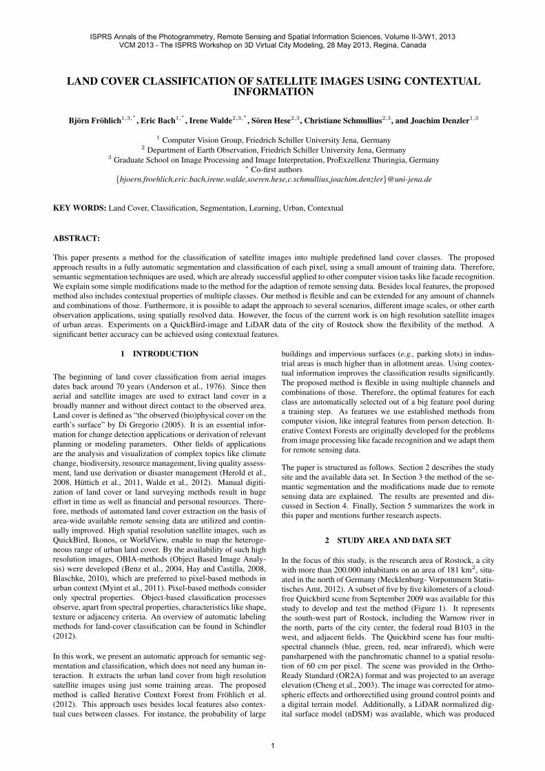
In the focus of this study, is the research area of Rostock, a citywith more than 200.000 inhabitants on an area of 181 km2, situ-ated in the north of Germany (Mecklenburg- Vorpommern Statis-tisches Amt, 2012). A subset of five by five kilometers of a cloud-free Quickbird scene from September 2009 was available for thisstudy to develop and test the method (Figure 1). It representsthe south-west part of Rostock, including the Warnow river inthe north, parts of the city center, the federal road B103 in thewest, and adjacent fields. The Quickbird scene has four multi-spectral channels (blue, green, red, near infrared), which werepansharpened with the panchromatic channel to a spatial resolu-tion of 60 cm per pixel. The scene was provided in the Ortho-Ready Standard (OR2A) format and was projected to an averageelevation (Cheng et al., 2003). The image was corrected for atmo-spheric effects and orthorectified using ground control points anda digital terrain model. Additionally, a LiDAR normalized dig-ital surface model (nDSM) was available, which was produced

ISPRS Annals of the Photogrammetry, Remote Sensing and Spatial Information Sciences, Volume II-3/W1, 2013VCM 2013 - The ISPRS Workshop on 3D Virtual City Modeling, 28 May 2013, Regina, Canada

1

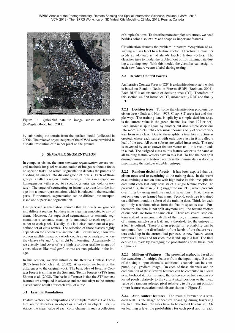
Figure 1: Quickbird satellite image subset of Rostock( c©DigitalGlobe, Inc., 2011).

by subtracting the terrain from the surface model (collected in2006). The relative object heights of the nDSM were provided ina spatial resolution of 2 m per pixel on the ground.

3 SEMANTIC SEGMENTATION

In computer vision, the term semantic segmentation covers sev-eral methods for pixel-wise annotation of images without a focuson specific tasks. At which, segmentation denotes the process ofdividing an images into disjoint group of pixels. Each of thosegroups is called a region. Furthermore, all pixels in a region arehomogeneous with respect to a specific criteria (e.g., color or tex-ture). The target of segmenting an image is to transform the im-age into a better representation, which is reduced to the essentialparts. Furthermore, segmentation can be differed into unsuper-vised and supervised segmentation.

Unsupervised segmentation denotes that all pixels are groupedinto different regions, but there is no meaning annotated to any ofthem. However, for supervised segmentation or semantic seg-mentation a semantic meaning is annotated to each region orrather to each pixel. Usually, this is a class name out of a pre-defined set of class names. The selection of those classes highlydepends on the chosen task and the data. For instance, a low res-olution satellite image of a whole country can be analyzed, wherethe classes city and forest might be interesting. Alternatively, ifwe classify land cover of very high resolution satellite images ofcities, classes like roof, pool, or tree are recognizable in the im-age.

In this section, we will introduce the Iterative Context Forest(ICF) from Frohlich et al. (2012). Afterwards, we focus on thedifferences to the original work. The basic idea of Iterative Con-text Forest is similar to the Semantic Texton Forests (STF) fromShoton et al. (2008). The basic difference is that the STF contextfeatures are computed in advance and can not adapt to the currentclassification result after each level of a tree.

3.1 Essential foundations

Feature vectors are compositions of multiple features. Each fea-ture vector describes an object or a part of an object. For in-stance, the mean value of each color channel is such a collection

of simple features. To describe more complex structures, we needbesides color also texture and shape as important features.

Classification denotes the problem in pattern recognition of as-signing a class label to a feature vector. Therefore, a classifierneeds an adequate set of already labeled feature vectors. Theclassifier tries to model the problem out of this training data dur-ing a training step. With this model, the classifier can assign toeach new feature vector a label during testing.

3.2 Iterative Context Forests

An Iterative Context Forests (ICF) is a classification system whichis based on Random Decision Forests (RDF) (Breiman, 2001).Each RDF is an ensemble of decision trees (DT). Therefore, inthis section we first introduce DT, subsequently RDF and finallyICF.

3.2.1 Decision trees To solve the classification problem, de-cision trees (Duda and Hart, 1973, Chap. 8.2) are a fast and sim-ple way. The training data is split by a simple decision (e.g.,is the current value in the green channel less than 127 or not).Each subset is split again by another but also simple decisionsinto more subsets until each subset consists only of feature vec-tors from one class. Due to these splits, a tree like structure iscreated, where each subset with only one class in it is called aleaf of the tree. All other subsets are called inner node. The treeis traversed by an unknown feature vector until this vector endsin a leaf. The assigned class to this feature vector is the same asall training feature vectors have in this leaf. To find the best splitduring training a brute-force search in the training data is done bymaximizing the Kullback-Leibler entropy.

3.2.2 Random decision forests It has been exposed that de-cision trees tend to overfitting to the training data. In the worstcase, training a tree on data with high noise let this tree split thedata until each leaf only consists of a single feature vector. Toprevent this, Breiman (2001) suggest to use RDF, which preventsoverfitting by using multiple random selections. First, there isnot only one tree learned but many. Second, each tree is trainedon a different random subset of the training data. Third, for eachsplit only a random subset from the feature space is used. Fur-thermore, the data is not split anymore until the feature vectorsof one node are from the same class. There are several stop cri-teria instead: a maximum depth of the tree, a minimum numberof training samples in a leaf, and a threshold for the entropy ina leaf is defined. Therefore, an a-posteriori probability can becomputed from the distribution of the labels of the feature vec-tors ended up in the current leaf per tree. A new feature vectortraverses all trees and for each tree it ends up in a leaf. The finaldecision is made by averaging the probabilities of all these leafs(Figure 2).

3.2.3 Millions of features The presented method is based onthe extraction of multiple features from the input image. Besidesof the single input channels, additional channels can be com-puted, e.g., gradient image. On each of these channels and oncombination of those several features can be computed in a localneighborhood d. For instance, the difference of two random se-lected pixels relatively to the current pixel position or the meanvalue of a random selected pixel relatively to the current position(more feature extraction methods are shown in Figure 3).

3.2.4 Auto context features The main difference to a stan-dard RDF is the usage of features changing during traversingthe tree. Therfore, the trees have to be created level-wise. Af-ter learning a level the probabilities for each pixel and for each


2

Figure 2: Random decision forest — l different binary decisiontree, traversed node are marked red and the reached leafs aremarked black.

class are added to the feature space as additional feature channels.Context knowledge can be extracted from the neighborhood, ifthe output of the previous level leads to an adequate result. Someof these contextual features are presented in Figure 8.

3.3 Modifications for remote sensing data

The presented method is only used before on datasets presentingfacade images (Frohlich et al., 2012). The challenges in facadeimages are different to the challenges in remote sensing images.Due to the resolution of the image and the size of the area, theobjects are much smaller compared to windows or other objectsfrom facade images. To adapt to this circumstances, the windowsize d is reduced (cf. Section 3.2.3 and Figure 3). Furthermore,some feature channels from the original work are not adaptableto remote sensing data, like the geometric context (Hoiem et al.,2005). Instead, some for the classical computer vision unusualchannels can be used. These channels are near infrared and Li-DAR nDSM. Due to the flexibility of the proposed method, anykind of channels might be added, like the “Normalized DifferenceVegetation Index” (NDVI):

NDVI(x, y) =NIR(x, y)− Red(x, y)

NIR(x, y) + Red(x, y). (1)

This index is computed from the red and the near infrared channeland allows a differentiation of vegetation and paved areas.

4 RESULTS

For testing, we used some already labeled training areas. On therest of the dataset 65 points per class are randomly selected fortesting (Figure 4). Due to the previous mentioned randomiza-tions, each classification is repeated ten times and the results areaveraged. We focused on the classes: tree, water, bare soil, build-ing, grassland, and impervious.

All tests are made with a fixed window size d = 30px = 18m fornon-contextual features and d = 120px = 72m for all contextualfeatures. Those values are exposed to be optimal in previous tests.

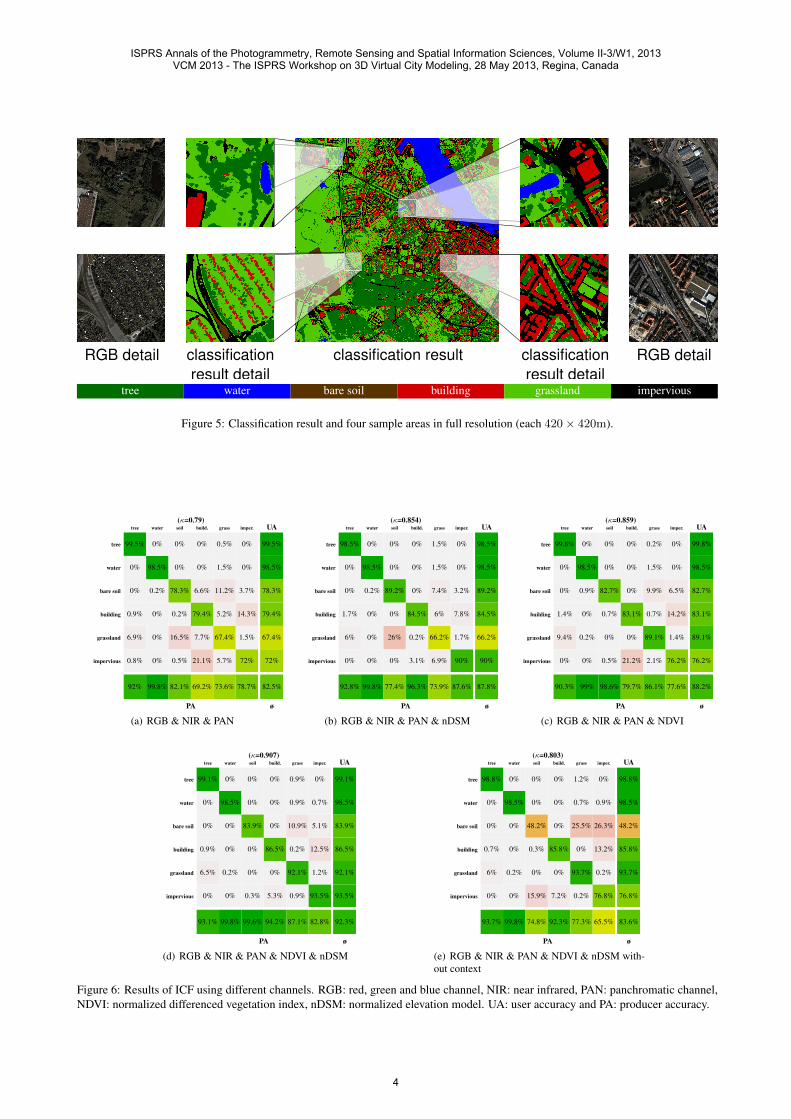
The qualitative results of our proposed method are presented inFigure 5 and the quantitative results in Figure 6. Using only theRGB values, the near infrared (NIR) and the panchromatic chan-nel (PAN) we get an overall accuracy of 82.5% (Figure 6(a)). Themain problems are to differ between the classes impervious andbuilding as well as grassland and bare soil. The classes tree andwater are already well classified. Adding the nDSM the confu-sion of building and impervious rapidly decreases (Figure 6(b)).This accords to our expectations, due to the fact that those bothclasses look very similar from the bird’s eye view but they differ

A

Bd

(a) pixel pair

d

(b) rectangle

d

(c) centered rectangle

d

AB

(d) diff. of two cent. rectan-gles

BA

d B

A

d

d

AB

A B

dB

A

d

(e) Haar-like (Viola and Jones, 2001)

Figure 3: Feature extraction methods from (Frohlich et al., 2012).The blue pixel denotes the current pixel position and the grid awindow around it. The red and orange pixels are used as fea-tures. They can be used as simple feature (c and d) or they can becombined, e.g., by A+B, A−B or |A−B| (a,b and e).

in the height. Adding the NDVI helps to reduce the confusionbetween the classes grassland and bare soil (Figure 6(c)). This isalso what we expected, due to the fact that grassland has a muchbrighter appearance in the NDVI image than bare soil. But thereare still some confusions between bare soil and grassland. On theother side, adding the NDVI also boosts the confusion betweentree and grassland. This might be a side effect of almost the sameappearance of those classes in the NDVI channel and the assign-ment of shrubs to either of the classes. In Figure 6(d), we addedboth channels, nDSM and NDVI. The benefits from adding onlyNDVI or adding only nDSM are still valid.

In Figure 6(e), we used the same settings as in Figure 6(d) besidesthat we switched off the context features. Almost every valuewithout using context is worse than the values using contextualcues. Especially, bare soil and impervious benefits from usingcontextual knowledge. Without contextual knowledge the classbare soil is often confused with grassland and impervious, butusing contextual knowledge impervious and bare soil are wellclassified. One suitable explanation for this might be that baresoil is often found on harvested fields outside the city. Due to thisreason, the probability for classes like grassland or impervious is


3

tree water bare soil building grassland impervious

Figure 5: Classification result and four sample areas in full resolution (each 420× 420m).

(κ=0.79)tree water soil build. grass imper.

impervious

grassland

building

bare soil

water

tree

0.8% 0% 0.5% 21.1% 5.7% 72%

6.9% 0% 16.5% 7.7% 67.4% 1.5%

0.9% 0% 0.2% 79.4% 5.2% 14.3%

0% 0.2% 78.3% 6.6% 11.2% 3.7%

0% 98.5% 0% 0% 1.5% 0%

99.5% 0% 0% 0% 0.5% 0%

UA

72%

67.4%

79.4%

78.3%

98.5%

99.5%

PA

92% 99.8% 82.1% 69.2% 73.6% 78.7%

ø

82.5%

(a) RGB & NIR & PAN


impervious

grassland

building

bare soil

water

tree

0% 0% 0% 3.1% 6.9% 90%

6% 0% 26% 0.2% 66.2% 1.7%

1.7% 0% 0% 84.5% 6% 7.8%

0% 0.2% 89.2% 0% 7.4% 3.2%

0% 98.5% 0% 0% 1.5% 0%

98.5% 0% 0% 0% 1.5% 0%

UA

90%

66.2%

84.5%

89.2%

98.5%

98.5%

PA

92.8% 99.8% 77.4% 96.3% 73.9% 87.6%

ø

87.8%

(b) RGB & NIR & PAN & nDSM


impervious

grassland

building

bare soil

water

tree

0% 0% 0.5% 21.2% 2.1% 76.2%

9.4% 0.2% 0% 0% 89.1% 1.4%

1.4% 0% 0.7% 83.1% 0.7% 14.2%

0% 0.9% 82.7% 0% 9.9% 6.5%

0% 98.5% 0% 0% 1.5% 0%

99.8% 0% 0% 0% 0.2% 0%

UA

76.2%

89.1%

83.1%

82.7%

98.5%

99.8%

PA

90.3% 99% 98.6% 79.7% 86.1% 77.6%

ø

88.2%

(c) RGB & NIR & PAN & NDVI


impervious

grassland

building

bare soil

water

tree

0% 0% 0.3% 5.3% 0.9% 93.5%

6.5% 0.2% 0% 0% 92.1% 1.2%

0.9% 0% 0% 86.5% 0.2% 12.5%

0% 0% 83.9% 0% 10.9% 5.1%

0% 98.5% 0% 0% 0.9% 0.7%

99.1% 0% 0% 0% 0.9% 0%

UA

93.5%

92.1%

86.5%

83.9%

98.5%

99.1%

PA

93.1% 99.8% 99.6% 94.2% 87.1% 82.8%

ø

92.3%

(d) RGB & NIR & PAN & NDVI & nDSM


impervious

grassland

building

bare soil

water

tree

0% 0% 15.9% 7.2% 0.2% 76.8%

6% 0.2% 0% 0% 93.7% 0.2%

0.7% 0% 0.3% 85.8% 0% 13.2%

0% 0% 48.2% 0% 25.5% 26.3%

0% 98.5% 0% 0% 0.7% 0.9%

98.8% 0% 0% 0% 1.2% 0%

UA

76.8%

93.7%

85.8%

48.2%

98.5%

98.8%

PA

93.7% 99.8% 74.8% 92.3% 77.3% 65.5%

ø

83.6%

(e) RGB & NIR & PAN & NDVI & nDSM with-out context

Figure 6: Results of ICF using different channels. RGB: red, green and blue channel, NIR: near infrared, PAN: panchromatic channel,NDVI: normalized differenced vegetation index, nDSM: normalized elevation model. UA: user accuracy and PA: producer accuracy.


4

impervious

iii ii

i iii

iiii

i

i

i i

i

ii

i

i

i

i

ii

i

i

i

i

ii

iiii

i

i

iii

ii

i

i

i

i

i i

i

i

i

i

i

ii

i

i

i

iii

i

i

i

i

i

i

i

i

i

i

i

ii

i

i

i

i

i

i

i

i

iii

i

i

i

ii

i i

i

i

i ii

i

ii

i

i

i

i

i

i

i

i

i

i

i

ii

i

i

ii

i

ii

i

ii

ii

i

i

i

i

ii

i

i

ii

ii

ii

i

i

i

ii

i

i

i

i

i

i

i i

i

i

i

ii

w

ww

w

w

w

ww

w

w

w

w

ww

w

w

ww

w

w

w

www

ww

ww

w

w

w

w w

w

ww

w

w

w

w w

ww

w

w

w

w

w

w

w

ww

w

w

w

w

ww

w

w

w

w

w

w

w

w

w

ww

ww w

w

w

ww

w

w

w

w

w

w

w

w

w

w

w

w

w

w

w

w

w

w

w

w

w

w

water

water

feature extraction trained split function result

input data d = 72m

input data d = 18mlocal context

loca

l fea

ture

loca

l fea

ture

global context (impervious vs. building)

i

i i

i

i

ii

i

i

i

ii

i

i

i

i

ii

iiii

i

i

iii

ii

i

i

i

i

i i

i

i

i

i

i

ii

i

i

i

iii

i

i

i

i

i

i

i

i

i

i

i

i

i

ii

i

i

i

i

i

i

i

i

iii

i

i

i

ii

i i

i

i

i

i

ii

i

ii

i

i

i

i

i

i

i

i

i i

i

i

ii

i

i

i

i

ii

i

i

ii

ii

ii

ii

ii

i

i

ii

i

ii

i

i

i

i

i

i

i

i

i

i

i

i

i

i ii

i

i

i

i

w

ww

ww w

ww

w

ww

w

ww

w

w

ww

w

www

www

w

ww

w

w

w

w w

w

ww

w

w

w

w w

w

w

w

w

w

w

w

ww

ww

w

w

w

ww

w

w

w

w

w ww

w

w

w

ww

ww

w w

w

w

ww

w

w

w

w

w

w

w

w

w

ww

w

w

w

w

w

ww

w

w

w

w

w

w

w

w w

w

ww

w

w

www

w

ww

w

i

i

i

i

ii

i i i

i

ii

ii

i

i i

i

i

i

i

ii

i

i

i

i

i

i

i

i

ii impervious

i i iii

i i i

i

i

i i iii

i i iii

i i iii

i i iii

Figure 7: Context vs. no context: first row using contextual features to differ between impervious (road) and water tends to betterresults than using no contextual features in the second row.

Figure 4: The seven training regions and the 65 evaluation pointsper class.

much higher in the neighborhood of buildings.

The influence of the window size and the usage of contextualfeatures is shown in Figure 7. In this example in the top row, theclasses water and impervious (the road) are well distinguished,but without using contextual knowledge there are some problemsin the bottom row, where some pixels in the middle of the streetare classified as water, due to the fact that in this case the sur-rounding area is not considered.

Since the time interval from LiDAR, collected in 2006, and theQuickBird satellite image, recorded in 2009, artificial “change”is created, which leads to misclassifications. Some buildings arevisible in the satellite image and not in the nDSM and the otherway around. There are some problems with the shadow of trees,which are not represented enough in the training data. Further-

more, small objects (like small detached houses) vanish in theclassification result with a larger window size. Finally, the objectborders are very smooth, this can be fixed by using an unsuper-vised segmentation.

In Figure 8, we show the final probability maps for all classesand for each pixel of selection of the data. It is not obligatory touse the most probable class per pixel as final decision. It is alsopossible to use those maps for further processing like filling gapsbetween streets. However, these specialized methods are not partof this work.

The best classification result (using context on the QuickBirddata, nDSM and NDVI) is shown in Figure 5, including someareas in detail.

5 CONCLUSIONS AND FURTHER WORK

In this work, we introduced a state of the art approach from com-puter vision for semantic segmentation. Furthermore, we havepresented how to adapt this method for the classification of landcover. In our experiment, we have shown that our method is flexi-ble in using multiple channels and that adding channels increasesthe quality of the result. The benefits of adding contextual knowl-edge to the classification has been demonstrated and discussed forsome specific problems.

For further work, we are planning to use an unsupervised seg-mentation to improve the performance especially at the bordersof the objects. Furthermore, we are planning to incorporate shapeinformation. Finally, an analysis of the whole QuickBird scene(13.8 × 15.5km) is planned as well as experiments using otherscales and classes.

ACKNOWLEDGMENTS

This work was partially founded by the ProExzellenz Initiativeof the “Thuringer Ministeriums fur Bildung, Wissenschaft undKultur” (TMBWK, grant no.: PE309-2). We also want to thankthe city of Rostock for providing the LiDAR data.


5

(a) RGB (b) result

(c) tree (d) water

(e) bare soil (f) building

(g) grassland (h) impervious

Figure 8: Probability maps for all classes (each sample area is840× 840m).

REFERENCES

Anderson, J. R., Hardy, E. E., Roach, J. T. and Witmer, R. E.,1976. A land use and land cover classification system for usewith remote sensor data.

Benz, U. C., Hofmann, P., Willhauck, G., Lingenfelder, I. andMarkus, H., 2004. Multi-resolution, object-oriented fuzzy analy-sis of remote sensing data for gis-ready information. ISPRS Jour-nal of Photogrammetry & Remote Sensing (58), pp. 239–258.

Blaschke, T., 2010. Object based image analysis for remote sens-ing. ISPRS Journal of Photogrammetry and Remote Sensing65(1), pp. 2–16.

Breiman, L., 2001. Random forests. Machine Learning 45(1),pp. 5–32.

Cheng, P., Toutin, T., Zhang, Y. and Wood, M., 2003. Quickbird –geometric correction, path and block processing and data fusion.Earth Observation Magazine 12(3), pp. 24–28.Di Gregorio, A., 2005. Land cover classification system softwareversion 2: Based on the orig. software version 1. Environmentand natural resources series Geo-spatial data and information,Vol. 8, rev. edn, Rome.

Duda, R. O. and Hart, P. E., 1973. Pattern Classification andScene Analysis. Wiley.

Frohlich, B., Rodner, E. and Denzler, J., 2012. Semantic seg-mentation with millions of features: Integrating multiple cues ina combined random forest approach. In: Proceedings of the AsianConference on Computer Vision (ACCV).

Hay, G. J. and Castilla, G., 2008. Geographic object-based im-age analysis (geobia): A new name for a new discipline. In:T. Blaschke, S. Lang and G. Hay (eds), Object-based image anal-ysis, Springer, pp. 75–89.

Herold, M., Woodcock, C., Loveland, T., Townshend, J., Brady,M., Steenmans, C. and Schmullius, C., 2008. Land-cover obser-vations as part of a global earth observation system of systems(geoss): Progress, activities, and prospects. IEEE Systems Jour-nal 2(3), pp. 414–423.

Hoiem, D., Efros, A. A. and Hebert, M., 2005. Geometric contextfrom a single image. In: Proceedings of the International Confer-ence on Computer Vision (ICCV)), Vol. 1, IEEE, pp. 654–661.

Huttich, C., Herold, M., Wegmann, M., Cord, A., Strohbach, B.,Schmullius, C. and Dech, S., 2011. Assessing effects of temporalcompositing and varying observation periods for large-area land-cover mapping in semi-arid ecosystems: Implications for globalmonitoring. Remote Sensing of Environment 115(10), pp. 2445–2459.

Mecklenburg- Vorpommern Statistisches Amt, 2012.http://www.statistik-mv.de.

Myint, S. W., Gober, P., Brazel, A., Grossman-Clarke, S. andWeng, Q., 2011. Per-pixel vs. object-based classification of ur-ban land cover extraction using high spatial resolution imagery.Remote Sensing of Environment 115(5), pp. 1145–1161.

Schindler, K., 2012. An overview and comparison of smoothlabeling methods for land-cover classification. IEEE Transactionson Geosciences and Remote Sensing.

Shotton, J., Johnson, M. and Cipolla, R., 2008. Semantic textonforests for image categorization and segmentation. In: Proceed-ings of the Conference on Computer Vision and Pattern Recogni-tion (CVPR), pp. 1–8.

Viola, P. and Jones, M., 2001. Rapid object detection using aboosted cascade of simple features. In: Proceedings of the Con-ference on Computer Vision and Pattern Recognition (CVPR),Vol. 1, IEEE, pp. 511–518.

Walde, I., Hese, S., Berger, C. and Schmullius, C., 2012. Graph-based urban land use mapping from high resolution satellite im-ages. ISPRS Ann. Photogramm. Remote Sens. Spatial Inf. Sci.I-4, pp. 119–124.


6

land cover classification of satellite images using contextual information

Documents