l’anàlisi multivariant aplicada una eina classica i...

1 de 110

SEM, una eina classica i moderna perl’anàlisi multivariant aplicada

Albert SatorraUniversitat Pompeu Fabra

Departament d’Economia i Empresa

Seminari del Servei d’Estadística, UAB8 d’octubre, 2003

2 de 110

Temes que tractarem: o Un exemple: regressió amb errors a les variableso Elements bàsics de SEM o Estimació i Contrast o Robustesa asimptòtica o Tipus de models SEM

Anàlisi factorial“Path Analysis”Equacions simultànies Models de corbes de creixement

o Una aplicació de SEM a l’anàlisi de rendiments empresarials, dades de dos nivells

o Conclusions

3 de 110

Examples with Coupon data (Bagozzi, 1994)

4 de 110

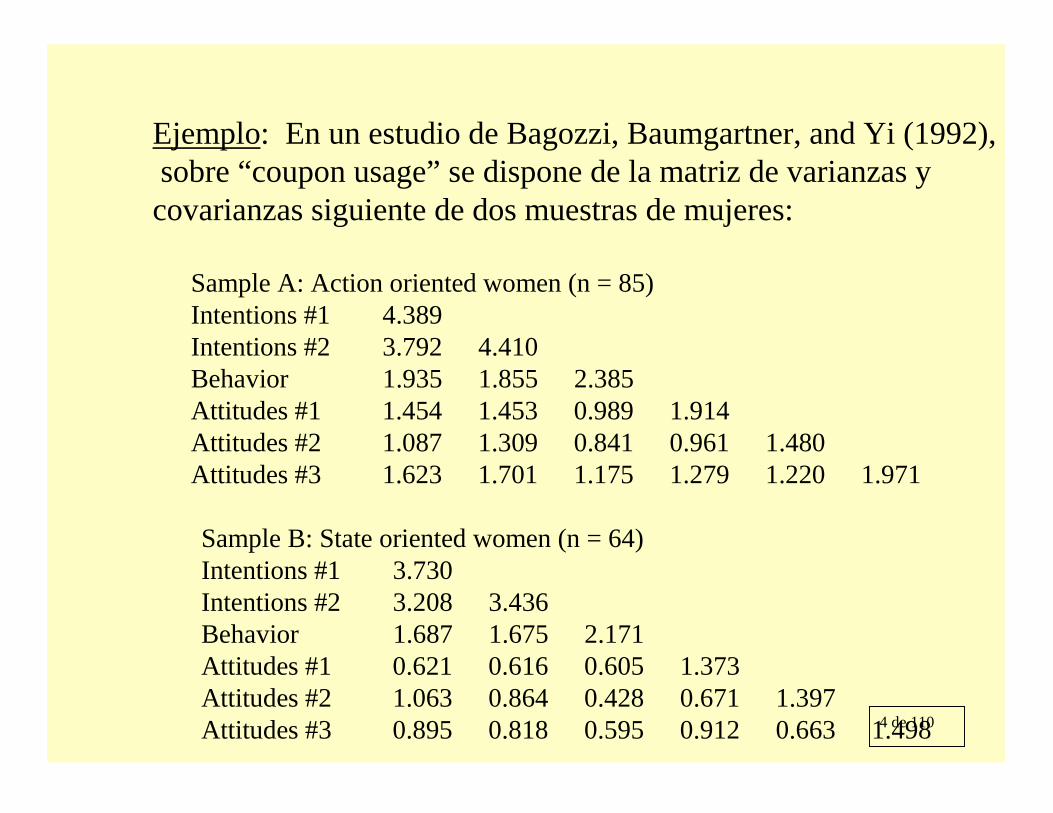
Ejemplo: En un estudio de Bagozzi, Baumgartner, and Yi (1992),sobre “coupon usage” se dispone de la matriz de varianzas y covarianzas siguiente de dos muestras de mujeres:

Sample A: Action oriented women (n = 85)Intentions #1 4.389Intentions #2 3.792 4.410Behavior 1.935 1.855 2.385Attitudes #1 1.454 1.453 0.989 1.914Attitudes #2 1.087 1.309 0.841 0.961 1.480Attitudes #3 1.623 1.701 1.175 1.279 1.220 1.971

Sample B: State oriented women (n = 64)Intentions #1 3.730Intentions #2 3.208 3.436Behavior 1.687 1.675 2.171Attitudes #1 0.621 0.616 0.605 1.373Attitudes #2 1.063 0.864 0.428 0.671 1.397Attitudes #3 0.895 0.818 0.595 0.912 0.663 1.498

5 de 110

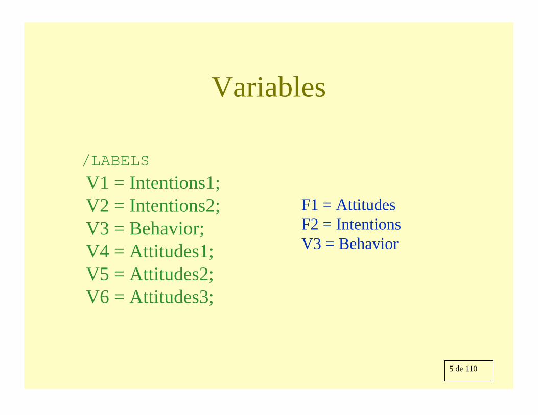
Variables

/LABELS

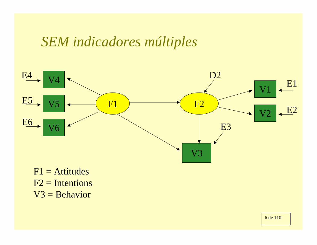
V1 = Intentions1; V2 = Intentions2;V3 = Behavior; V4 = Attitudes1; V5 = Attitudes2; V6 = Attitudes3;

F1 = AttitudesF2 = IntentionsV3 = Behavior

6 de 110

F1 F2

V3

D2

E3

SEM indicadores múltiples

V4

V5

V6

V1

V2

E4

E5

E6

E1

E2

F1 = AttitudesF2 = IntentionsV3 = Behavior

7 de 110

INTENTIO=V1 = 1.000 F2 + 1.000 E1

INTENTIO=V2 = 1.014*F2 + 1.000 E2

.088

11.585

BEHAVIOR=V3 = .330*F2 + .492*F1 + 1.000 E3

.103 .204

3.203 2.411

ATTITUDE=V4 = 1.020*F1 + 1.000 E4

.136

7.501

ATTITUDE=V5 = .951*F1 + 1.000 E5

.117

8.124

ATTITUDE=V6 = 1.269*F1 + 1.000 E6

.127

10.005

INTENTIO=F2 = 1.311*F1 + 1.000 D2

.214

6.116

VARIANCES OF INDEPENDENT VARIABLES----------------------------------

E D--- ---

E1 -INTENTIO .649*I D2 -INTENTIO 2.020*I.255 I .437 I2.542 I 4.619 I

I IE2 -INTENTIO .565*I I

.257 I I2.204 I I

I IE3 -BEHAVIOR 1.311*I I

.213 I I6.166 I I

I IE4 -ATTITUDE .875*I I

.161 I I5.424 I I


.115 I I5.023 I I


.132 I I2.729 I I

CHI-SQUARE = 5.426, 7 DEGREES OF FREEDOMPROBABILITY VALUE IS 0.60809

8 de 110

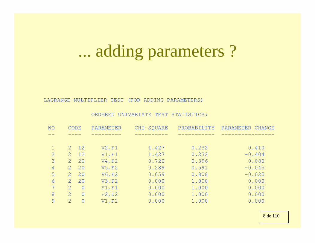
... adding parameters ?

LAGRANGE MULTIPLIER TEST (FOR ADDING PARAMETERS)

ORDERED UNIVARIATE TEST STATISTICS:

NO CODE PARAMETER CHI-SQUARE PROBABILITY PARAMETER CHANGE-- ---- --------- ---------- ----------- ----------------

1 2 12 V2,F1 1.427 0.232 0.4102 2 12 V1,F1 1.427 0.232 -0.4043 2 20 V4,F2 0.720 0.396 0.0804 2 20 V5,F2 0.289 0.591 -0.0455 2 20 V6,F2 0.059 0.808 -0.0256 2 20 V3,F2 0.000 1.000 0.0007 2 0 F1,F1 0.000 1.000 0.0008 2 0 F2,D2 0.000 1.000 0.0009 2 0 V1,F2 0.000 1.000 0.000

9 de 110

STRUCTURAL EQUATION MODELING

LINEAR STRUCTURAL RELATIONS

10 de 110

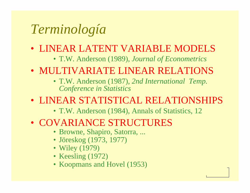
Terminología• LINEAR LATENT VARIABLE MODELS

• T.W. Anderson (1989), Journal of Econometrics

• MULTIVARIATE LINEAR RELATIONS• T.W. Anderson (1987), 2nd International Temp.

Conference in Statistics

• LINEAR STATISTICAL RELATIONSHIPS• T.W. Anderson (1984), Annals of Statistics, 12

• COVARIANCE STRUCTURES• Browne, Shapiro, Satorra, ...• Jöreskog (1973, 1977)• Wiley (1979)• Keesling (1972)• Koopmans and Hovel (1953)

11 de 110

Computer programs• LISREL• EQS• LISCOMP / Mplus• COSAN• MOMENTS• CALIS• AMOS• RAMONA• Mx

• Jöreskog and Sörbom• Bentler• Muthén• McDonalds• Schoenberg • SAS• Arbunckle• Browne • Neale

12 de 110

Computer programs and Web adresses

• SEM software: – EQS http://www.mvsoft.com– LISREL http://www.ssicentral.com– MPLUS http://www.statmodel.com/index2.html– AMOS http://smallwaters.com/amos/– Mx http://www.vipbg.vcu.edu/~vipbg/dr/MNEALE.shtml

� Web addresses of interest:SEMNET; http://www.gsu.edu/~mkteer/semfaq.html

Jason Newsom's SEM Reference Listhttp://www.ioa.pdx.edu/newsom/semrefs.htm

13 de 110

... books

• Bollen (1989)• Dwyer (1983)• Hayduk (1987)• Mueller (1996)• Saris and Stronkhorst (1984)• Dunn, Everitt and Pickles (1993)• ...

14 de 110

... many research papers

• Austin and Wolfle (1991): Annotated bibliography of structural equation modeling: Technical Works. BJMSP, 99, pp. 85-152.

• Austin, J.T. and Calteron, R.F. (1996). Theoretical and technical contributions to structural equation modeling: An updated annotated bibliography. SEM, pp. 105-175.

15 de 110

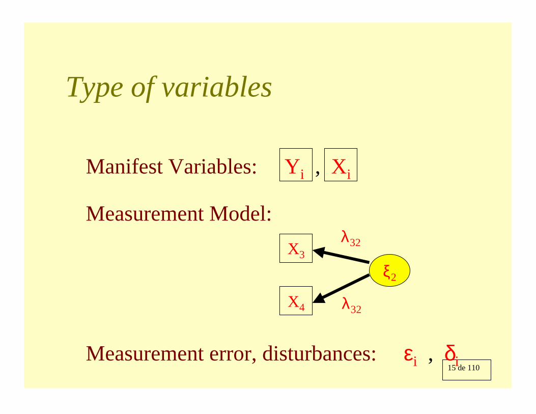
Type of variables

Manifest Variables: Yi , Xi

Measurement Model:

ξ2

X3

X4

λ32

λ32

Measurement error, disturbances: εi , δi

16 de 110

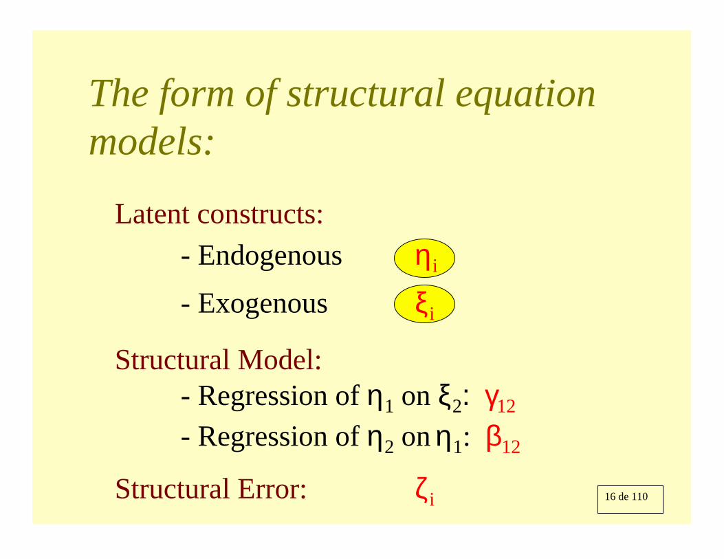
The form of structural equation models:

Latent constructs:- Endogenous ηi

- Exogenous ξi

Structural Model:- Regression of η1 on ξ2: γ12

- Regression of η2 on η1: β12

Structural Error: ζi

17 de 110

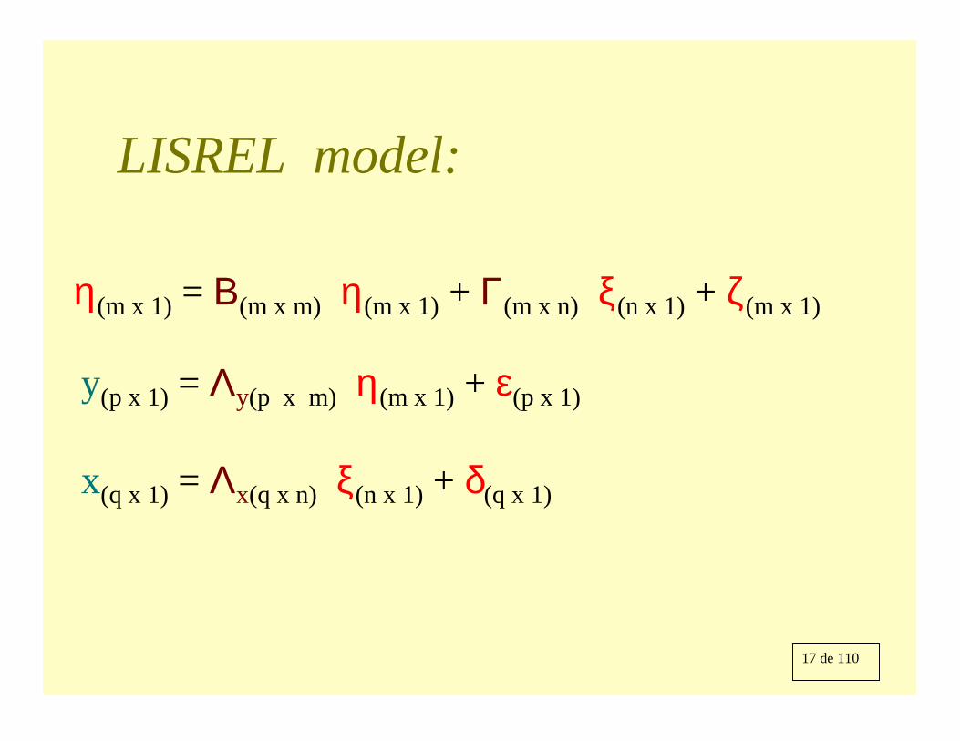
LISREL model:

η(m x 1) = Β(m x m) η(m x 1) + Γ(m x n) ξ(n x 1) + ζ(m x 1)

y(p x 1) = Λy(p x m) η(m x 1) + ε(p x 1)

x(q x 1) = Λx(q x n) ξ(n x 1) + δ(q x 1)

18 de 110

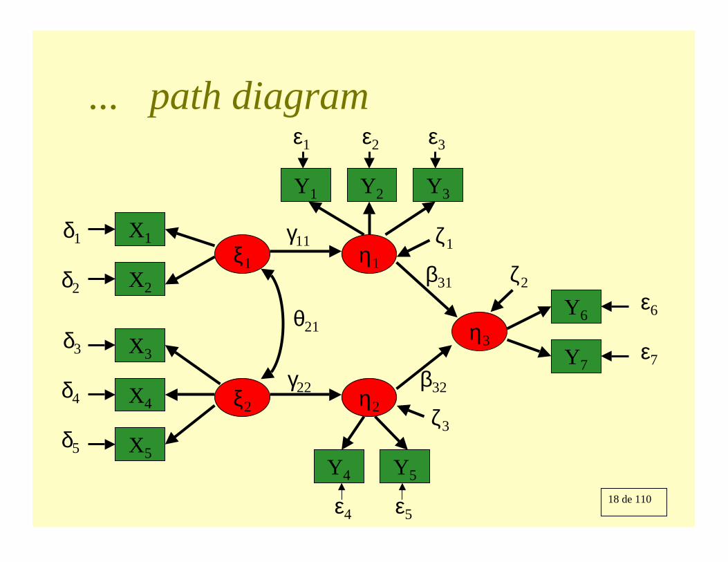
... path diagram

X1

X2

X3

X4

X5

ξ1

ξ2

η1

η2

η3

Y6

Y7

Y1 Y2 Y3

Y4 Y5

γ11

γ22

β31

β32

ζ1

ζ2

ζ3

θ21

δ1

δ2

δ3

δ4

δ5

ε1 ε2 ε3

ε6

ε7

ε4 ε5

19 de 110

Aspects of SEM1. Substantive theory

– Concepts– Constructs– Formalization

2. Basic Issues– Causality– Model building

• Theory Driven vs Data Driven– Exploratory vs Confirmatory Analysis– Units of measurement and Standardization– Scale Types

20 de 110

Aspects of SEM3. Statistical

– Statistical Specification of Model– Identification of Models and Parameters– Fitting and Testing of Model

• Assessment of Fit• Detection of Specification Errors

– Sequential Model Fitting– Testing Structural Hypothesis

4. Computational

21 de 110

Main virtues of SEM

• Unifies several multivariate methods into one analytic framework

• Allows for latent variables in a statistical model and measurement error

• Expresses the effects of latent variables on each other and the effect of latent variables on observed variables

• Allows testing substantive hypothesis involving causal relationships among construct or latent variables

22 de 110

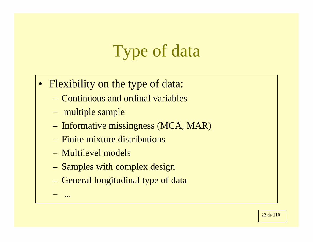
Type of data

• Flexibility on the type of data: – Continuous and ordinal variables– multiple sample– Informative missingness (MCA, MAR) – Finite mixture distributions – Multilevel models– Samples with complex design – General longitudinal type of data– ...

23 de 110

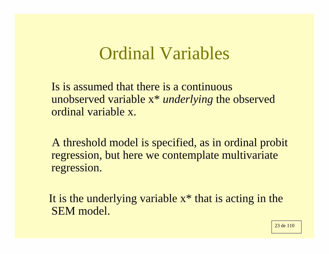
Ordinal Variables

Is is assumed that there is a continuous unobserved variable x* underlying the observed ordinal variable x.

A threshold model is specified, as in ordinal probitregression, but here we contemplate multivariateregression.

It is the underlying variable x* that is acting in the SEM model.

24 de 110

A multiple group SEM: model and statistical analysis

25 de 110

Introducción a SEM:

• Datos: • Matriz de datos (“raw data”)• Estadísticos suficientes (medias muestrales, varianzas y

covarianzas)

Matrizdatos

(n x p)

Indiv.

vars

Momentos Muestrales::• Vector de medias• Matriz S de var. y cov. (p x p)• Matriz de momentos de cuarto orden: Γ (p* x p*) p* = p(p+1)/2, p=20--> p* =210

26 de 110

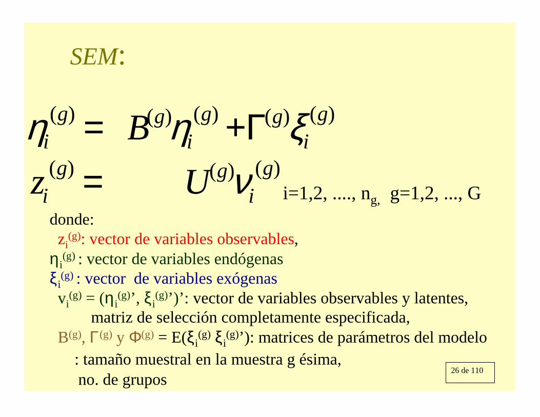
SEM:

)()()(

)()()()()(

gi

ggi

gi

ggi

ggi

UzB

νξηη

=Γ+=

i=1,2, ...., ng, g=1,2, ..., G donde:zi

(g): vector de variables observables, ηi

(g) : vector de variables endógenasξi

(g) : vector de variables exógenasvi

(g) = (ηi(g)’, ξi

(g)’)’: vector de variables observables y latentes, U(g): matriz de selección completamente especificada, B(g), Γ(g) y Φ(g) = E(ξi

(g) ξi(g)’): matrices de parámetros del modelo

ng : tamaño muestral en la muestra g ésima, G: no. de grupos

27 de 110

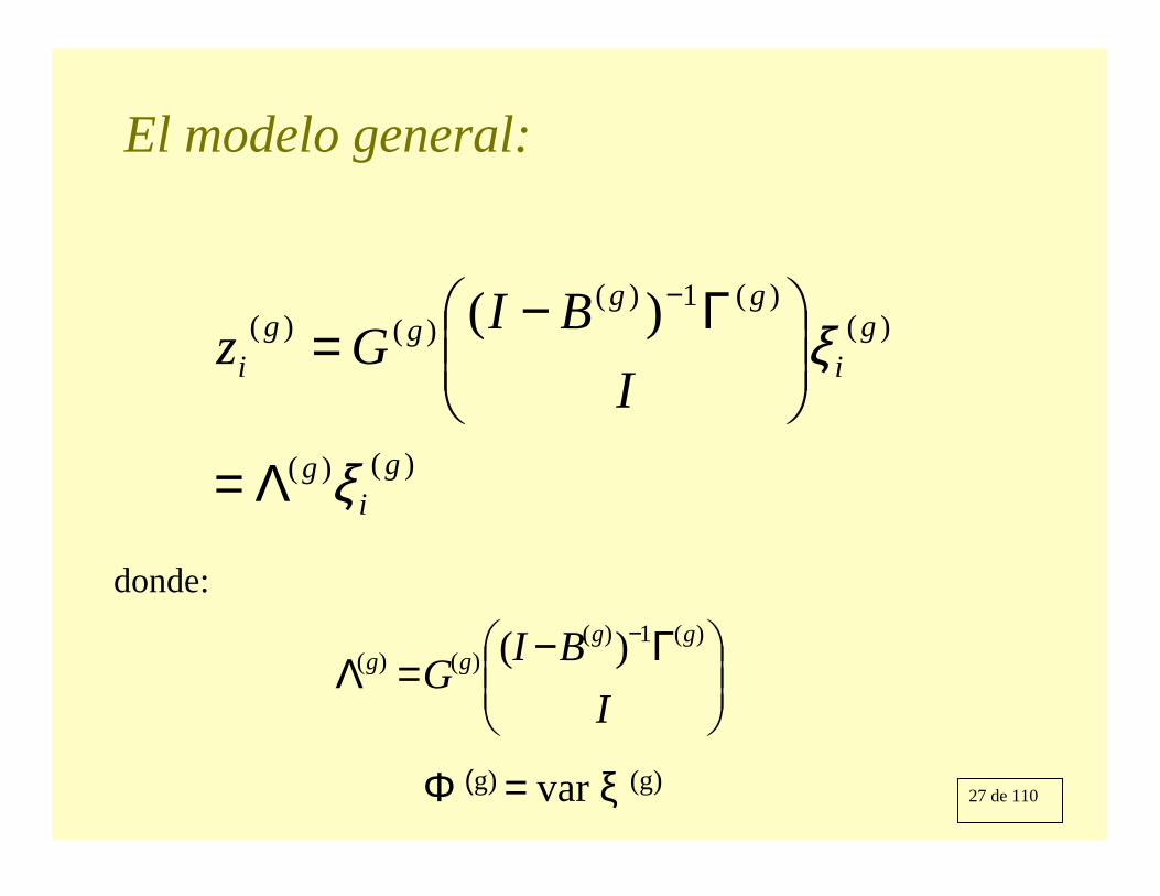
El modelo general:

)()(

)()(1)(

)()( )(

gi

g

gi

gggg

i IBI

Gz

ξ

ξ

Λ=

Γ−=

−

Γ−=Λ

−

IBI

Ggg

gg)(1)(

)()( )(donde:

Φ

(g) = var ξ (g)

28 de 110

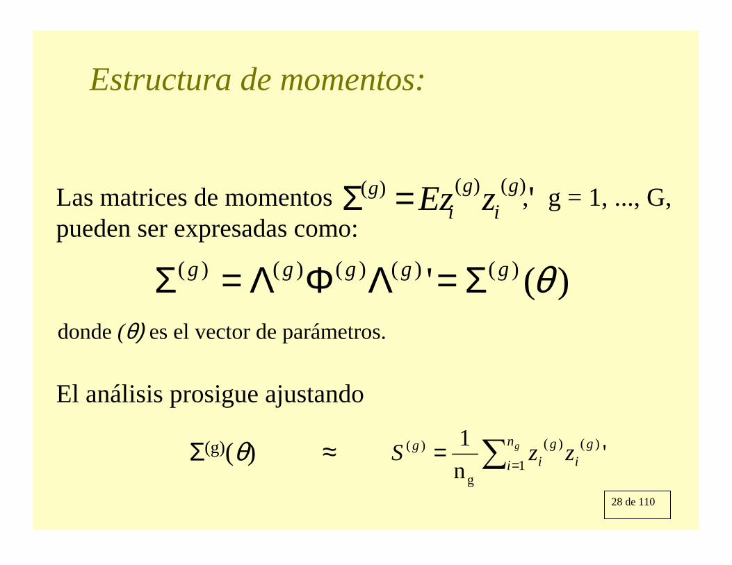
Estructura de momentos:

Las matrices de momentos , g = 1, ..., G, pueden ser expresadas como:

)(' )()()()()( θggggg Σ=ΛΦΛ=Σ

El análisis prosigue ajustando

Σ(g)(θ) ≈ ∑ == gn

ig

ig

ig zzS

1)()(

g

)( 'n1

donde (θ) es el vector de parámetros.

')()()( gi

gi

g zEz=Σ

29 de 110

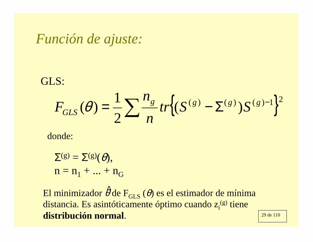
GLS:

{ }∑−Σ−= 21)()()( )(

21)( gggg

GLS SStrnn

F θ

donde:

Σ(g) = Σ(g)(θ),n = n1 + ... + nG

El minimizador θ de FGLS (θ) es el estimador de mínima distancia. Es asintóticamente óptimo cuando zi

(g) tienedistribución normal.

^

Función de ajuste:

30 de 110

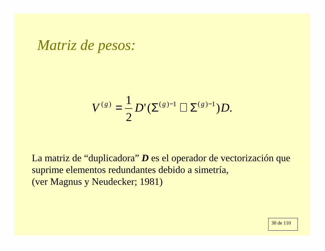
Matriz de pesos:

.)('21 1)(1)()( DDV ggg −− Σ⊗Σ=

La matriz de “duplicadora” D es el operador de vectorización que suprime elementos redundantes debido a simetría, (ver Magnus y Neudecker; 1981)

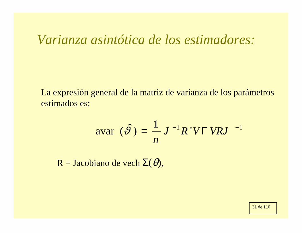
31 de 110

Varianza asintótica de los estimadores:

11 '1)ˆ(avar −− Γ= VRJVRJn

ϑ

La expresión general de la matriz de varianza de los parámetrosestimados es:

R = Jacobiano de vech Σ(θ),

32 de 110

Varianzas asintóticas de los momentos:

ΓΓ=Γ )(

)()1(

)1(ˆ,,ˆdiagˆ G

Gnn

nn

…

∑=−

=Γ)(

1

)()()(

)(

11ˆ

gn

i

gi

gig

g hhn

donde

)')((vech )()()()()( ggi

ggi

gi szszh −−= )()( vech gg Ss =y

con

La expresión general del estimador de Γ es

33 de 110

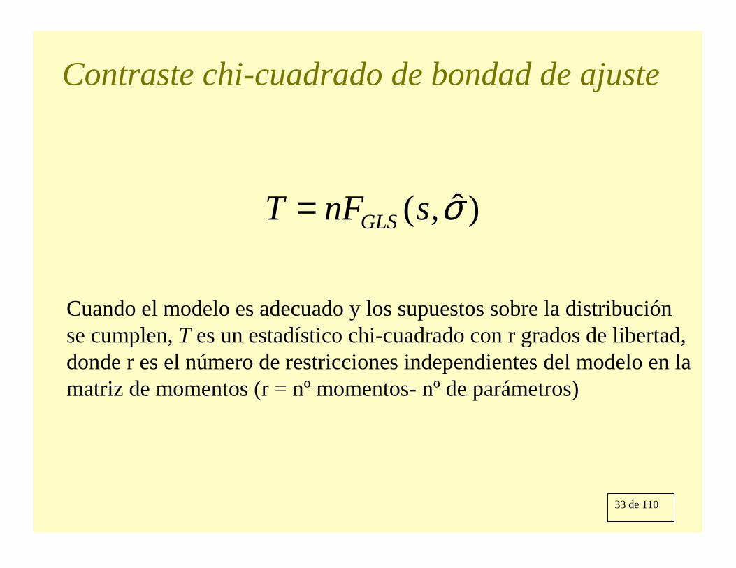
Contraste chi-cuadrado de bondad de ajuste

Cuando el modelo es adecuado y los supuestos sobre la distribución se cumplen, T es un estadístico chi-cuadrado con r grados de libertad, donde r es el número de restricciones independientes del modelo en la matriz de momentos (r = nº momentos- nº de parámetros)

)ˆ,( σsnFT GLS=

34 de 110

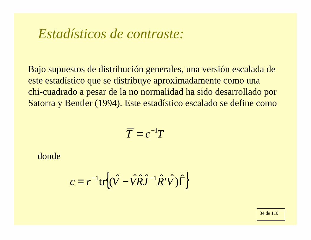
Estadísticos de contraste:

Bajo supuestos de distribución generales, una versión escalada de este estadístico que se distribuye aproximadamente como una chi-cuadrado a pesar de la no normalidad ha sido desarrollado por Satorra y Bentler (1994). Este estadístico escalado se define como

TcT 1−=

{ }Γ−= −− ˆ)ˆ'ˆˆˆˆˆ(tr 11 VRJRVVrc

donde

35 de 110

SEM BASIC MODELS

Factor analysis

36 de 110

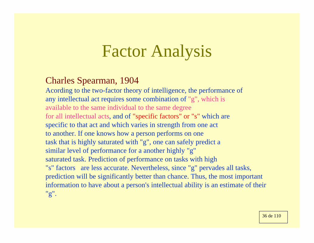
Factor AnalysisCharles Spearman, 1904Acording to the two-factor theory of intelligence, the performance of any intellectual act requires some combination of "g", which is available to the same individual to the same degreefor all intellectual acts, and of "specific factors" or "s" which are specific to that act and which varies in strength from one act to another. If one knows how a person performs on onetask that is highly saturated with "g", one can safely predict asimilar level of performance for a another highly "g" saturated task. Prediction of performance on tasks with high "s" factors are less accurate. Nevertheless, since "g" pervades all tasks, prediction will be significantly better than chance. Thus, the most important information to have about a person's intellectual ability is an estimate of their "g".

37 de 110

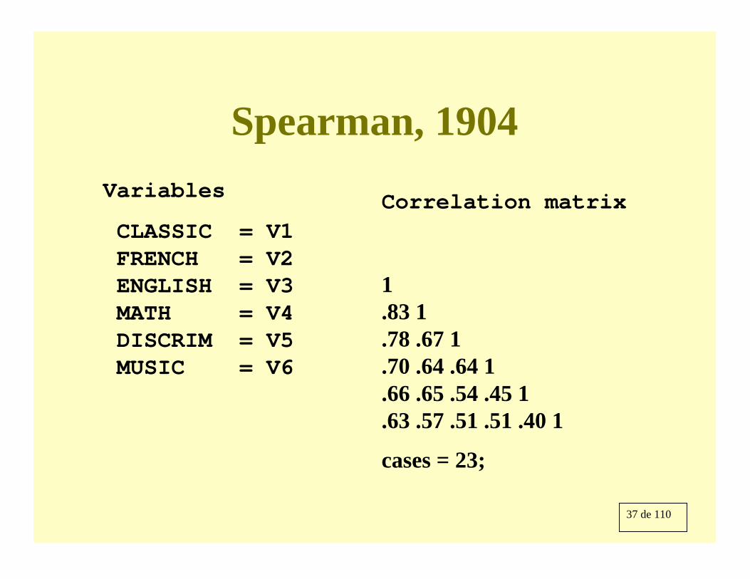
Spearman, 1904Variables

CLASSIC = V1FRENCH = V2ENGLISH = V3MATH = V4DISCRIM = V5MUSIC = V6

Correlation matrix

1.83 1.78 .67 1.70 .64 .64 1.66 .65 .54 .45 1.63 .57 .51 .51 .40 1

cases = 23;

38 de 110

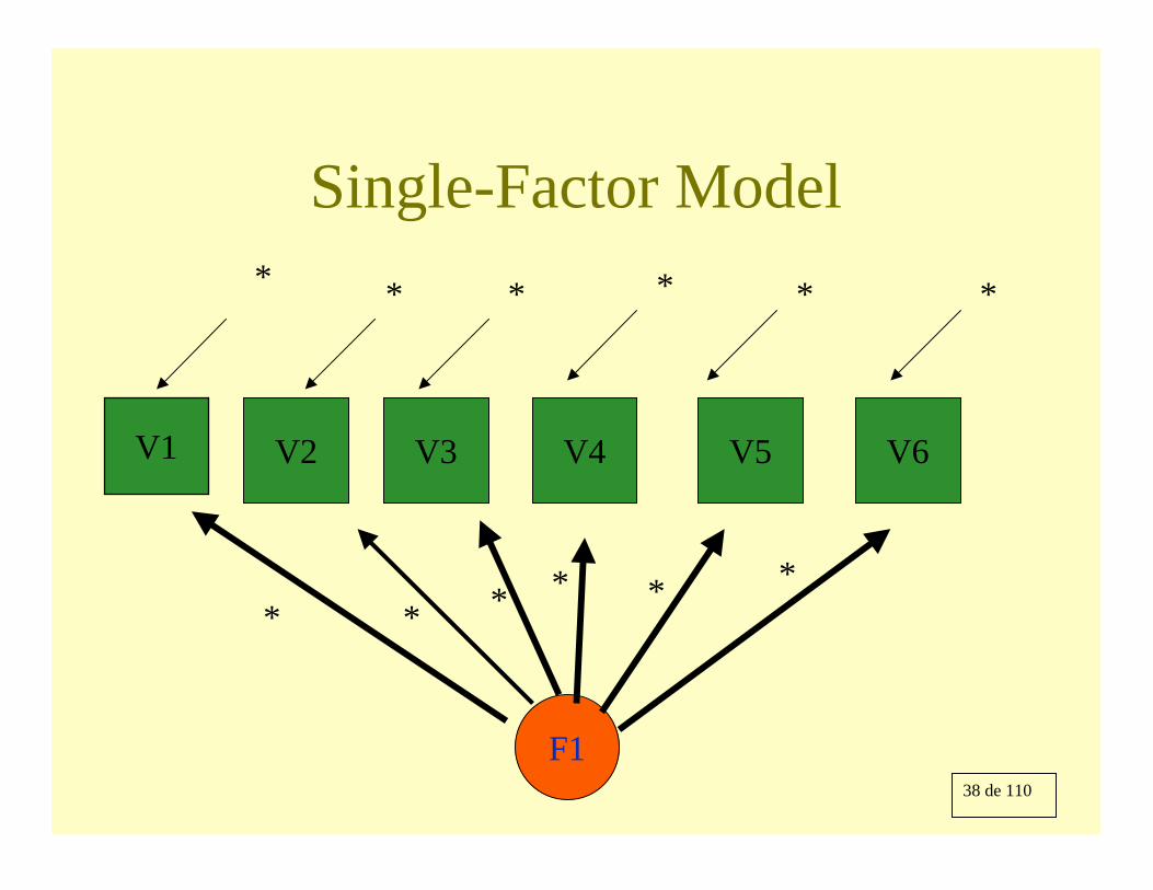
Single-Factor Model

V1 V4V3V2

F1

* * * *

* * * *

V6V5

**

**

39 de 110

EQS code for a factor model /Title confirmatory factor analysis: 1 factor ! (Spearman, 1904 ) eqs/exer3.eqs/Specifications var = 6; cases = 23;/Label v1 = classic; v2 = french; v3 =english; v4 = math; V5 = discrim;V6=music;/equationsV1 = *f1 + e1;V2 = *f1+ e2;V3 = *f1 + e3;V4 = *f1 + e4;V5 = *f1 + e5;V6 = *f1 + e6;/variances f1 = 1; e1 to e6 = *;/matrix1.83 1.78 .67 1.70 .64 .64 1.66 .65 .54 .45 1.63 .57 .51 .51 .40 1/LMTEST/end

40 de 110

NT analysis

RESIDUAL COVARIANCE MATRIX (S-SIGMA) :

CLASSIC FRENCH ENGLISH MATH DISCRIMV 1 V 2 V 3 V 4 V 5

CLASSIC V 1 0.000FRENCH V 2 -0.001 0.000ENGLISH V 3 0.005 -0.029 0.000

MATH V 4 -0.006 0.003 0.046 0.000DISCRIM V 5 -0.001 0.054 -0.015 -0.056 0.000MUSIC V 6 0.003 0.005 -0.017 0.030 -0.049

MUSICV 6

MUSIC V 6 0.000

CHI-SQUARE = 1.663 BASED ON 9 DEGREES OF FREEDOMPROBABILITY VALUE FOR THE CHI-SQUARE STATISTIC IS 0.99575THE NORMAL THEORY RLS CHI-SQUARE FOR THIS ML SOLUTION IS 1.648

.

41 de 110

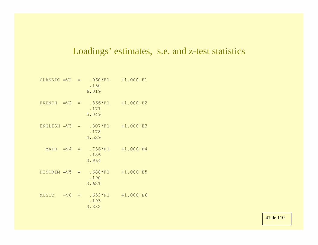
Loadings’ estimates, s.e. and z-test statistics

CLASSIC =V1 = .960*F1 +1.000 E1.160

6.019

FRENCH =V2 = .866*F1 +1.000 E2.171

5.049

ENGLISH =V3 = .807*F1 +1.000 E3.178

4.529

MATH =V4 = .736*F1 +1.000 E4.186

3.964

DISCRIM =V5 = .688*F1 +1.000 E5.190

3.621

MUSIC =V6 = .653*F1 +1.000 E6.193

3.382

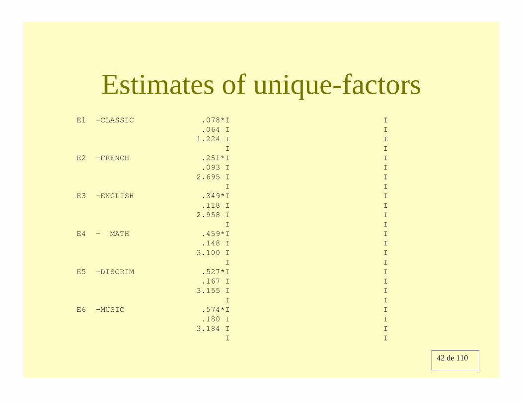
42 de 110

Estimates of unique-factors E1 -CLASSIC .078*I I

.064 I I1.224 I I

I IE2 -FRENCH .251*I I

.093 I I2.695 I I

I IE3 -ENGLISH .349*I I

.118 I I2.958 I I

I IE4 - MATH .459*I I

.148 I I3.100 I I

I IE5 -DISCRIM .527*I I

.167 I I3.155 I I

I IE6 -MUSIC .574*I I

.180 I I3.184 I I

I I

43 de 110

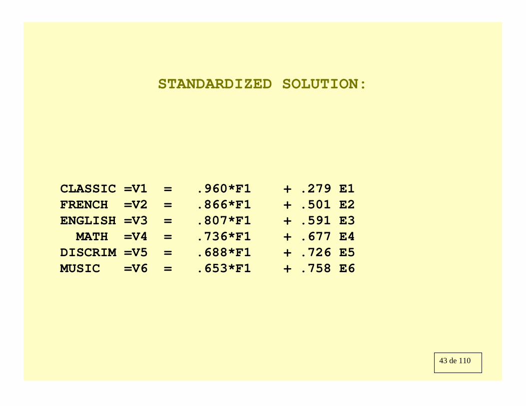
STANDARDIZED SOLUTION:

CLASSIC =V1 = .960*F1 + .279 E1FRENCH =V2 = .866*F1 + .501 E2ENGLISH =V3 = .807*F1 + .591 E3MATH =V4 = .736*F1 + .677 E4

DISCRIM =V5 = .688*F1 + .726 E5MUSIC =V6 = .653*F1 + .758 E6

44 de 110

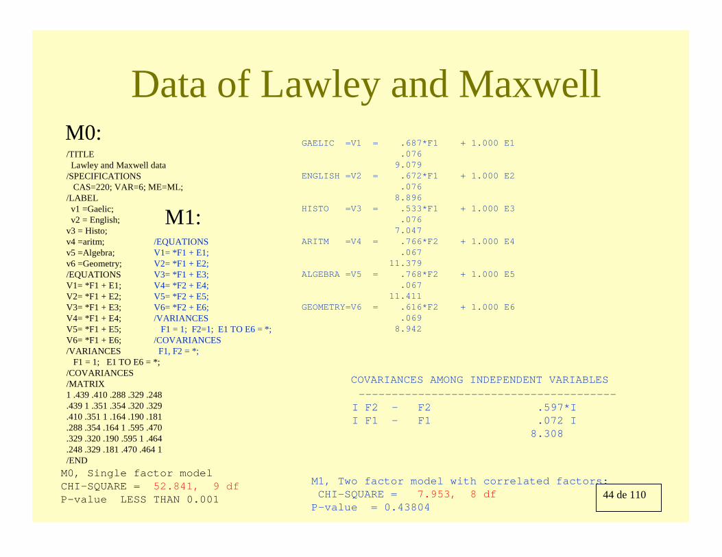
Data of Lawley and Maxwell/TITLE

Lawley and Maxwell data /SPECIFICATIONS

CAS=220; VAR=6; ME=ML;/LABEL

v1 =Gaelic;v2 = English;

v3 = Histo;v4 =aritm;v5 =Algebra;v6 =Geometry; /EQUATIONSV1= *F1 + E1;V2= *F1 + E2; V3= *F1 + E3; V4= *F1 + E4; V5= *F1 + E5; V6= *F1 + E6;/VARIANCES

F1 = 1; E1 TO E6 = *;/COVARIANCES/MATRIX1 .439 .410 .288 .329 .248.439 1 .351 .354 .320 .329.410 .351 1 .164 .190 .181.288 .354 .164 1 .595 .470.329 .320 .190 .595 1 .464.248 .329 .181 .470 .464 1/END

/EQUATIONSV1= *F1 + E1;V2= *F1 + E2; V3= *F1 + E3; V4= *F2 + E4; V5= *F2 + E5; V6= *F2 + E6;/VARIANCES

F1 = 1; F2=1; E1 TO E6 = *;/COVARIANCES

F1, F2 = *;

GAELIC =V1 = .687*F1 + 1.000 E1.076

9.079ENGLISH =V2 = .672*F1 + 1.000 E2

.0768.896

HISTO =V3 = .533*F1 + 1.000 E3.076

7.047ARITM =V4 = .766*F2 + 1.000 E4

.06711.379

ALGEBRA =V5 = .768*F2 + 1.000 E5.067

11.411GEOMETRY=V6 = .616*F2 + 1.000 E6

.0698.942

COVARIANCES AMONG INDEPENDENT VARIABLES

---------------------------------------I F2 - F2 .597*II F1 - F1 .072 I

8.308

M0:

M1:

M0, Single factor modelCHI-SQUARE = 52.841, 9 dfP-value LESS THAN 0.001

M1, Two factor model with correlated factors:CHI-SQUARE = 7.953, 8 df

P-value = 0.43804

45 de 110

Monte Carlo Evaluation

> Single sample, one-factor model

Asymptotic Robustness

46 de 110

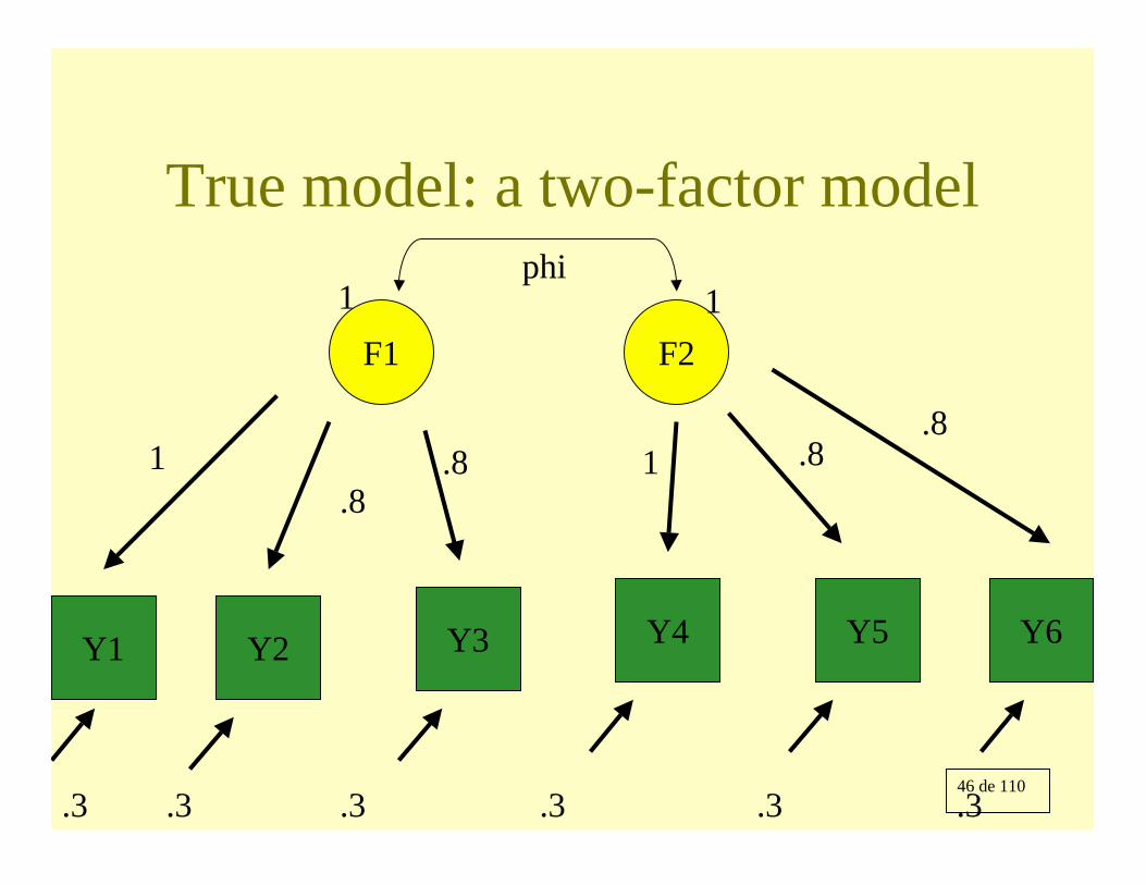
True model: a two-factor model

Y2 Y5Y4Y3

F1 F2

1 .8 1 .8

phi

.3 .3.3.3

Y1 Y6

.3.3

.8

.8

1 1

47 de 110

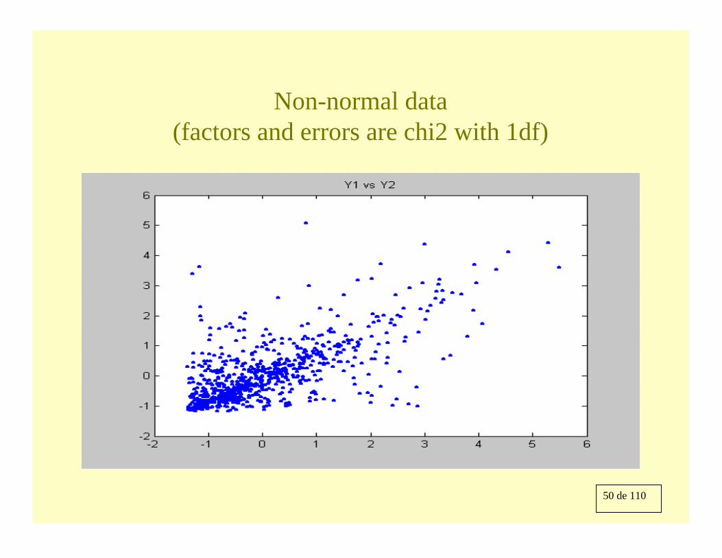
Distribution of factors and errors

• F1, F2 non-normal, chi2 of 1 df, transformed to be of variance 1 and with thedesired correlation phi.

• Errors are independent chi2 of 1 df scaled tohave the desired variance, .3.

48 de 110

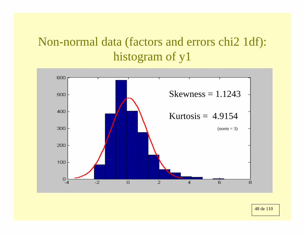
Non-normal data (factors and errors chi2 1df): histogram of y1

Skewness = 1.1243

Kurtosis = 4.9154(norm = 3)

49 de 110

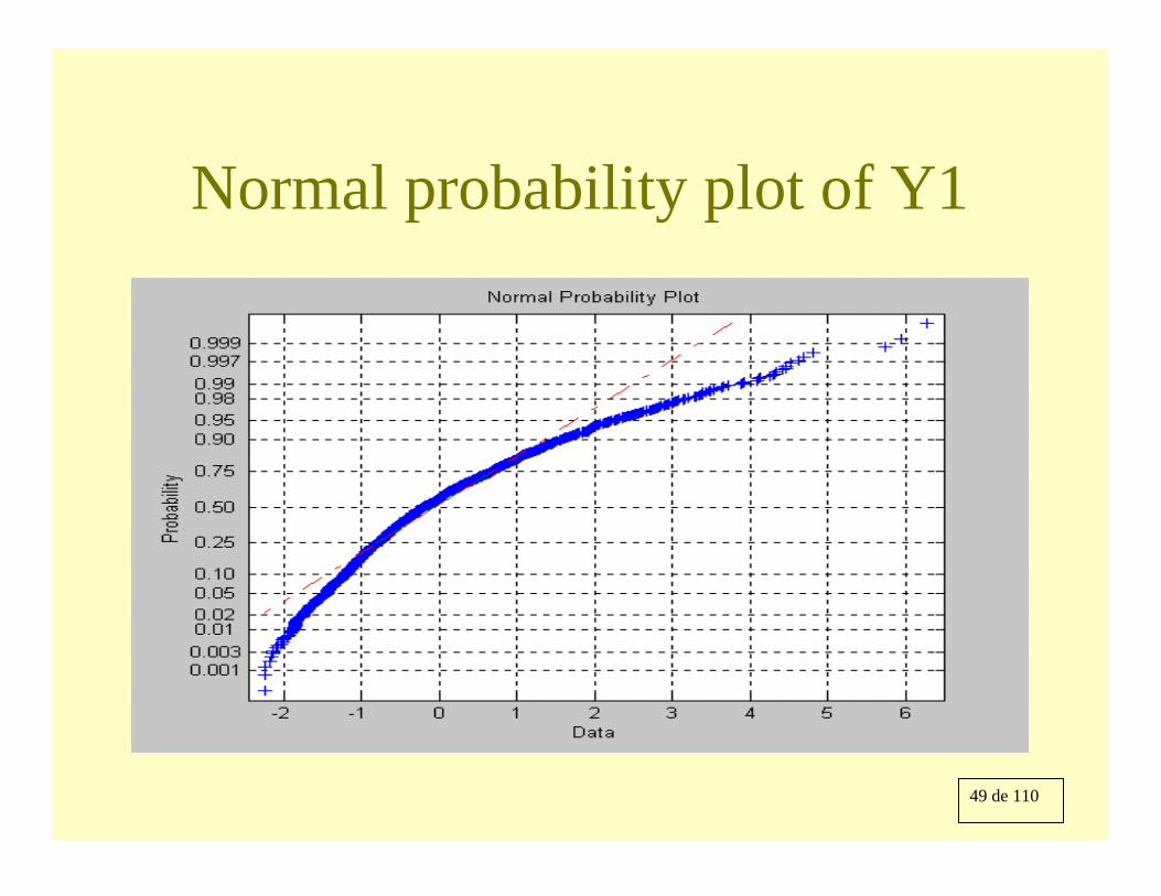
Normal probability plot of Y1

50 de 110

Non-normal data (factors and errors are chi2 with 1df)

51 de 110

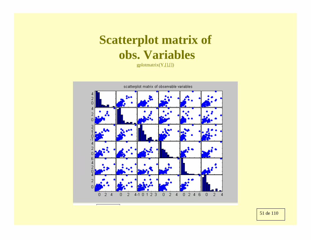
Scatterplot matrix ofobs. Variables

gplotmatrix(Y,[],[])

52 de 110

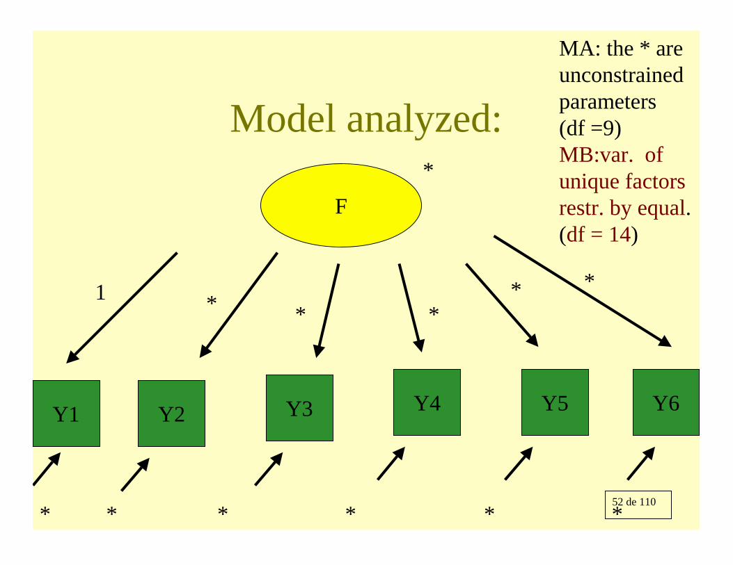
Model analyzed:

Y2 Y5Y4Y3

1 *

* ***

Y1 Y6

**

*

F

* * *

*

MA: the * are unconstrained parameters (df =9)MB:var. of unique factors restr. by equal.(df = 14)

53 de 110

A case where H0 holdsbut two different models:

df = 9 or 14

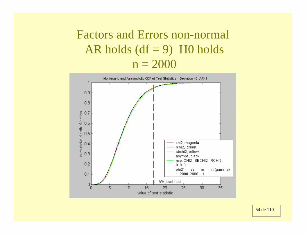
54 de 110

Factors and Errors non-normal AR holds (df = 9) H0 holds

n = 2000

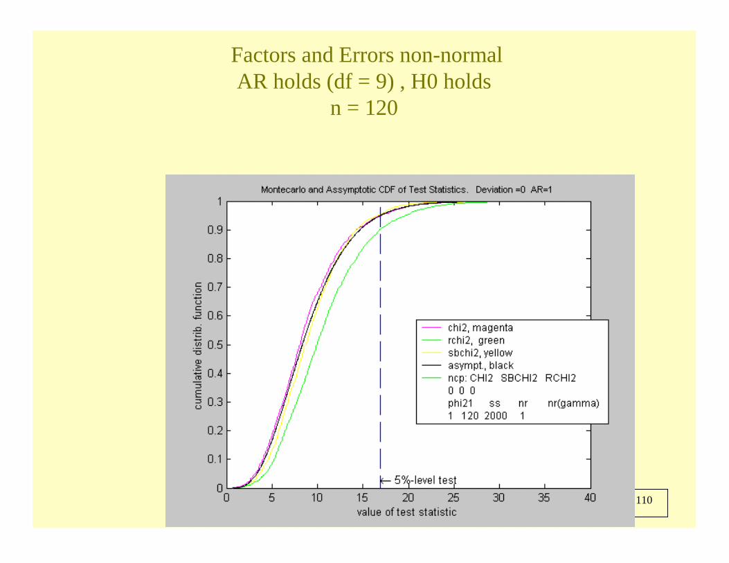
55 de 110

Factors and Errors non-normalAR holds (df = 9) , H0 holds

n = 120

56 de 110

Factors and Errors non-normalnon-AR ( df = 14), H0 holds

n = 2000

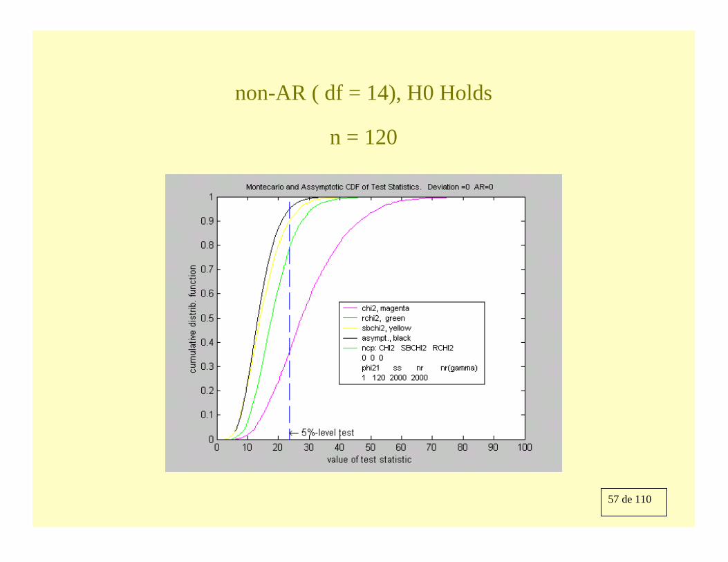
57 de 110

non-AR ( df = 14), H0 Holds

n = 120

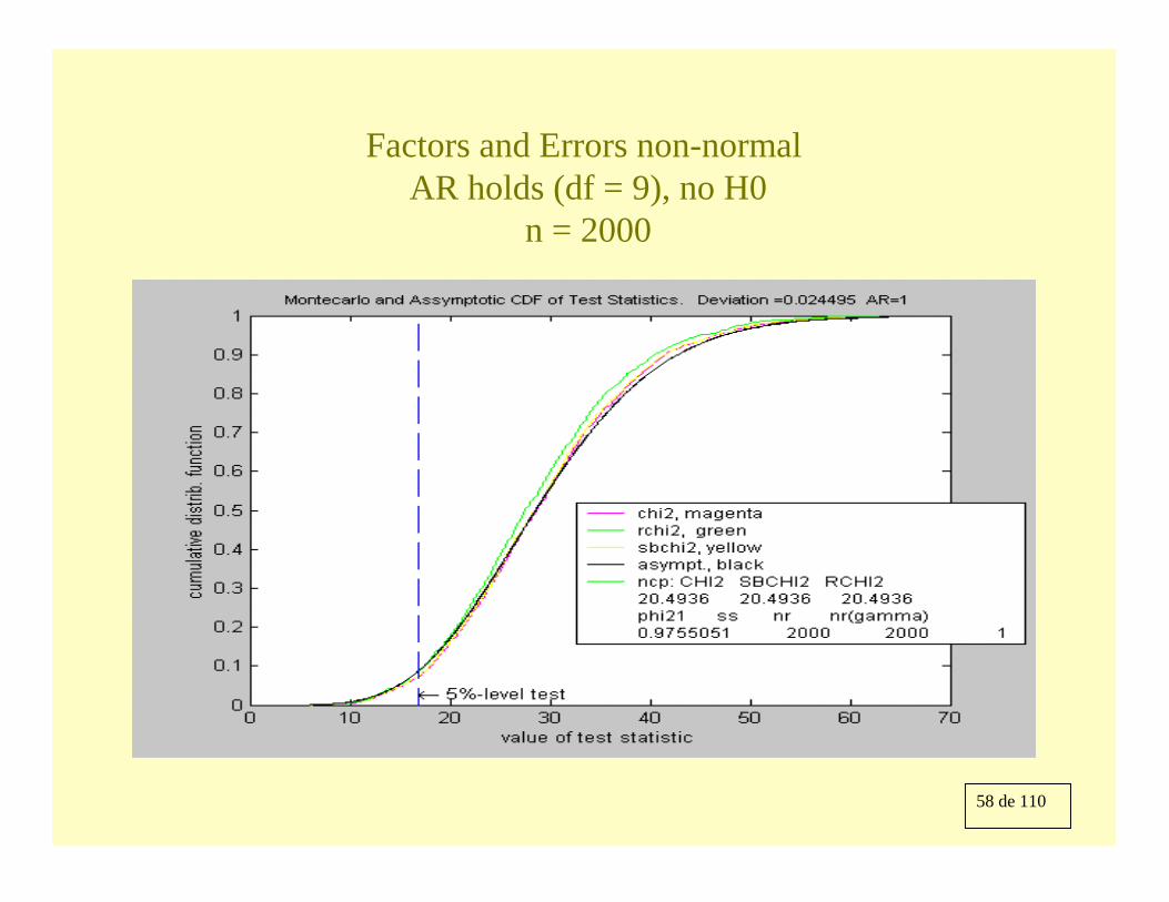
58 de 110

Factors and Errors non-normal AR holds (df = 9), no H0

n = 2000

59 de 110

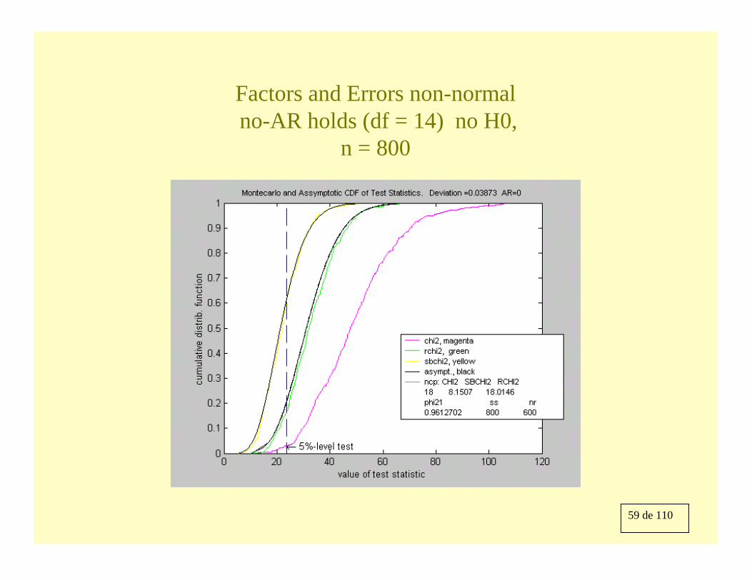
Factors and Errors non-normal no-AR holds (df = 14) no H0,

n = 800

60 de 110

Simultaneous equations

61 de 110

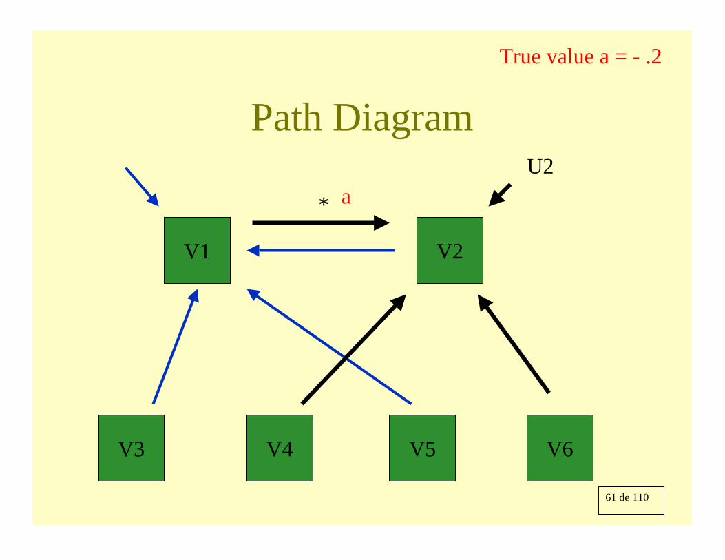
Path Diagram

V1

V5V4V3

V2

V6

U2

* a

True value a = - .2

62 de 110

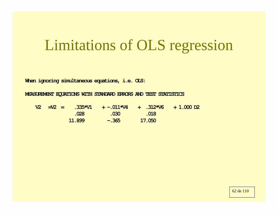
Limitations of OLS regression

When ignoring simultaneous equations, i.e. OLS:

MEASUREMENT EQUATIONS WITH STANDARD ERRORS AND TEST STATISTICS

V2 =V2 = .335*V1 + -.011*V4 + .312*V6 + 1.000 D2.028 .030 .018

11.899 -.365 17.050

63 de 110

EQS analysis:

GOODNESS OF FIT SUMMARY

/TITLEexample of SEM

/SPECIFICATIONSCASES = 500 ; VAR = 6;/EQUATIONSV1 = .5*V2 + *V3 + *V5 +D1 ;V2 = -.5*V1 + *V4 + *V6 + D2 ;/VARIANCESD1 = *;D2 = *;V3 = *; V4 = *; V5 = *; V6=*;/COVARIANCESV3 to V6 = *;

/MATRIX2.51230.9345 0.54141.4768 0.4544 1.59102.1110 0.6925 1.4842 2.10371.5067 0.5093 0.5278 1.4727 1.55660.3683 0.4155 -0.0683 0.0235 0.0847

0.9376/END

64 de 110

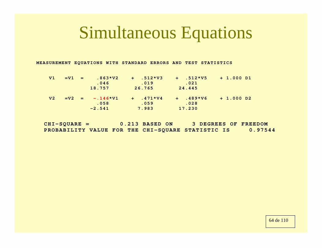
Simultaneous EquationsMEASUREMENT EQUATIONS WITH STANDARD ERRORS AND TEST STATISTICS

V1 =V1 = .863*V2 + .512*V3 + .512*V5 + 1.000 D1.046 .019 .021

18.757 26.765 24.445

V2 =V2 = -.146*V1 + .471*V4 + .489*V6 + 1.000 D2.058 .059 .028

-2.541 7.983 17.230

CHI-SQUARE = 0.213 BASED ON 3 DEGREES OF FREEDOMPROBABILITY VALUE FOR THE CHI-SQUARE STATISTIC IS 0.97544

65 de 110

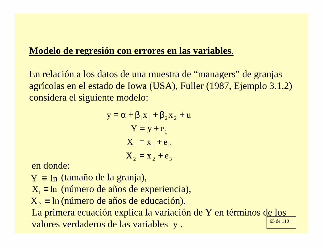
Modelo de regresión con errores en las variables.

En relación a los datos de una muestra de “managers” de granjas agrícolas en el estado de Iowa (USA), Fuller (1987, Ejemplo 3.1.2) considera el siguiente modelo:

322

211

1

2211

exXexX

eyYuxxy

+=+=

+=+β+β+α=

en donde:(tamaño de la granja), (número de años de experiencia),(número de años de educación).

La primera ecuación explica la variación de Y en términos de los valores verdaderos de las variables y .

lnY ≡lnX1 ≡lnX2 ≡

66 de 110

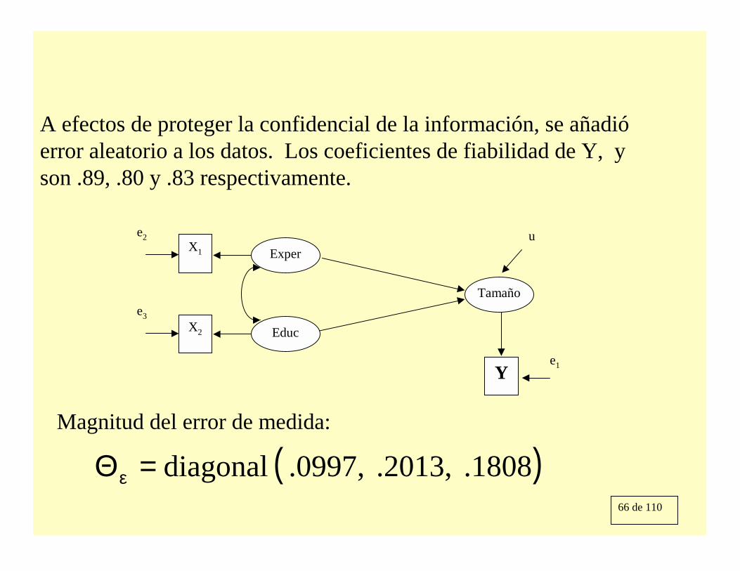
A efectos de proteger la confidencial de la información, se añadióerror aleatorio a los datos. Los coeficientes de fiabilidad de Y, y son .89, .80 y .83 respectivamente.

ExperX1

X2

u

Ye1

Educ

Tamaño

e2

e3

( ).1808 .2013, ,0997. diagonal=Θε

Magnitud del error de medida:

67 de 110

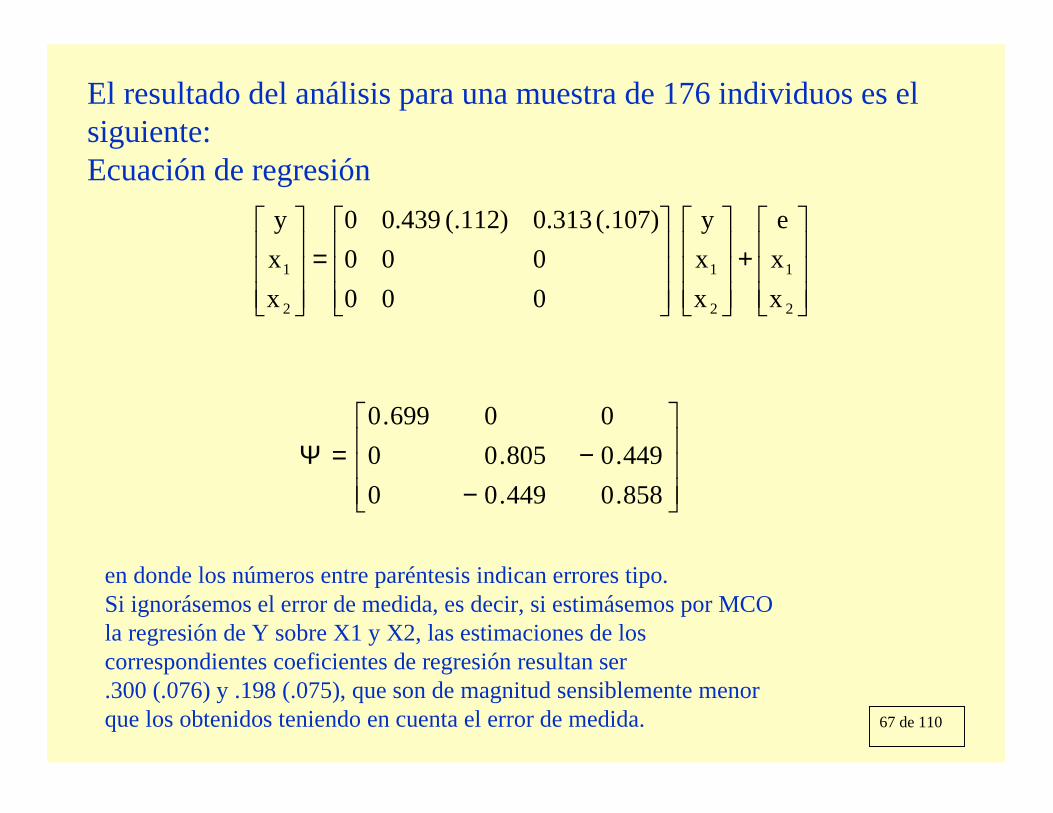
El resultado del análisis para una muestra de 176 individuos es el siguiente:Ecuación de regresión

+

=

2

1

2

1

2

1

xxe

xxy

000000

(.107) 313.0)112(. 439.00

xxy

−−=Ψ

858.0449.00449.0805.00

00699.0

en donde los números entre paréntesis indican errores tipo. Si ignorásemos el error de medida, es decir, si estimásemos por MCO la regresión de Y sobre X1 y X2, las estimaciones de los correspondientes coeficientes de regresión resultan ser .300 (.076) y .198 (.075), que son de magnitud sensiblemente menor que los obtenidos teniendo en cuenta el error de medida.

68 de 110

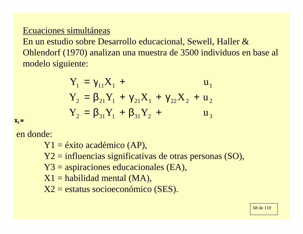
Ecuaciones simultáneasEn un estudio sobre Desarrollo educacional, Sewell, Haller & Ohlendorf (1970) analizan una muestra de 3500 individuos en base al modelo siguiente:

32311312

22221211212

11111

uYYYuXXYYuXY

+β+β=+γ+γ+β=

+γ=

en donde:Y1 = éxito académico (AP),Y2 = influencias significativas de otras personas (SO),Y3 = aspiraciones educacionales (EA),X1 = habilidad mental (MA),X2 = estatus socioeconómico (SES).

≡1Y ≡2Y ≡3Y ≡1X ≡2X

69 de 110

y2

u2

X1

X2

Y1

Y3

Y2

u3

e2

La ecuación de medida será:

+

=

000

e0

XXYyY

1000001000001000001000001

XXYYY

2

2

1

3

2

1

2

1

3

2

1

( )0,0,0*,,0diagonal=Θε

El modelo propuesto impone 2 restricciones de sobreidentificación obteniéndosechi2=7.14. Sin introducir error de medida en Y2, el valor del estadístico chi-cuadrado es 186.39 con 3 df, valor extraordinariamente alto que conduce por tanto al rechazodel modelo que ignora error de medida.

70 de 110

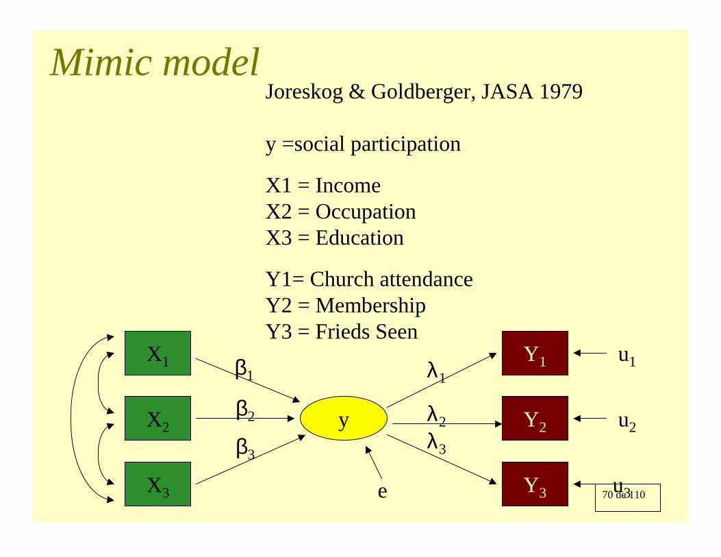
Mimic modelJoreskog & Goldberger, JASA 1979

y =social participation

X1 = IncomeX2 = OccupationX3 = Education

Y1= Church attendanceY2 = MembershipY3 = Frieds Seen

y

X1

X2

X3

Y1

Y2

Y3e

u2

u3

u1β1

β2

β3

λ1

λ2λ3

71 de 110

Mimic model

+

⋅

=

3

2

1

3

2

1

3

2

13

2

11

3

2

1

3

2

1

100001000010000000000

hhhuuu

XXXy

XXXYYY

λλλ

+

⋅

∗∗∗

=

3

2

1

3

2

1

3

2

1

000000000000

0

XXXe

XXXy

XXXy

~ Ψ

∗∗

∗

00

00

0

~ Φ* 0

0 *

72 de 110

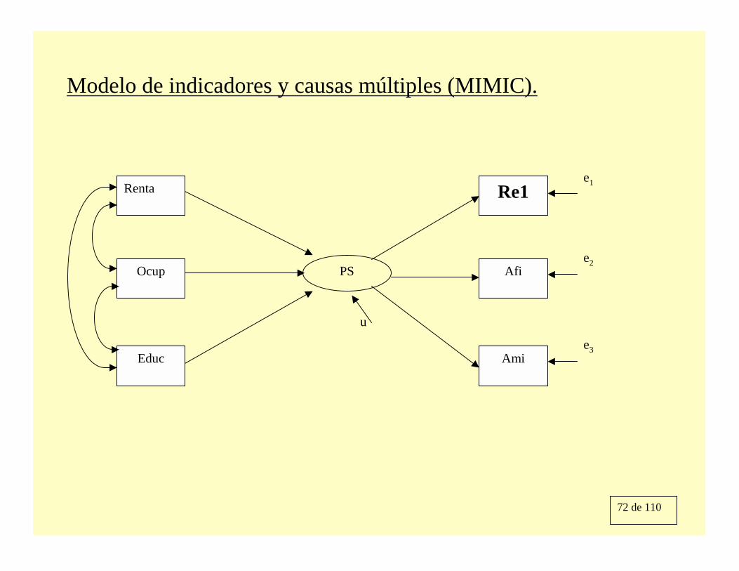
Modelo de indicadores y causas múltiples (MIMIC).

PS

e1Renta

Ocup

Educ

e2

Re1

Afi

Amie3

u

73 de 110

Utilizando el método de estimación de la máxima verosimilitud, obtenemos las siguientes estimaciones:

(.046)ey 346.Y

(.060)ey 634.Y

)046(.ey 402.Y

)070(.)065(.)066(.uX 386.X 114.X 269.y

33

22

11

321

+=

+=

+=

+++=

Un aspecto a destacar aquí es que el modelo en cuestión impone 6 restricciones de sobreidentificación sobre la matriz de varianzas y covarianzas de las variables observables. El correspondiente estadístico es igual a 12.36 con un “P-VALUE” igual a 0.052.

74 de 110

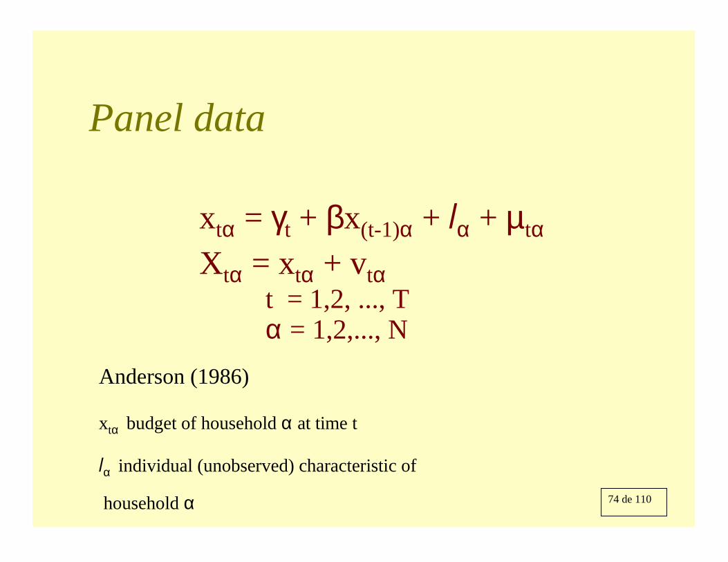
Panel data

xtα = γt + βx(t-1)α + lα + µtα

Xtα = xtα + vtαt = 1,2, ..., Tα = 1,2,..., N

Anderson (1986)

xtα budget of household α at time t

lα individual (unobserved) characteristic of

household α

75 de 110

Panel data

+

⋅

=

01000001000001000001000001

4

3

2

1

1

4

3

2

1

1

4

3

2

1

vvvv

lxxxx

lXXXX

~ Ψ

+

⋅

+

=

1

4

3

2

1

1

4

3

2

1

5

3

2

1

1

4

3

2

1

0000010001000100000000

0 llxxxx

lxxxx

µµµµ

ββ

β

γγγγ ~ Φ

76 de 110

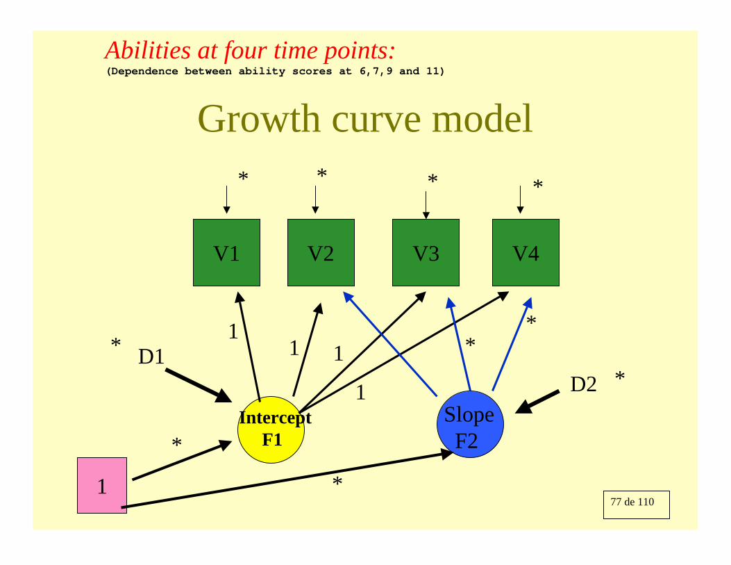
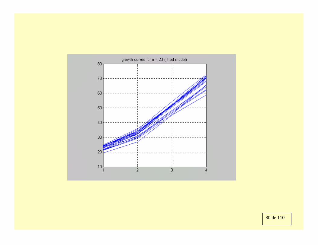
Growth curve model

77 de 110

Growth curve model

V1 V4V3V2

11 1

1Intercept

F1SlopeF2

**

* ***

1

D2D1

**

*

*

Abilities at four time points:(Dependence between ability scores at 6,7,9 and 11)

78 de 110

Estimates

ABIL6 =V1 = 1.000 F1 + 1.000 E1

ABIL7 =V2 = 1.000 F1 + 1.000 F2 + 1.000 E2

ABIL9 =V3 = 1.000 F1 + 2.187*F2 + 1.000 E3.069

31.739

ABIL11 =V4 = 1.000 F1 + 3.656*F2 + 1.000 E4.119

30.755

INTERCEP=F1 = 18.042*V999 + 1.000 D1.470

38.417

SLOPE =F2 = 7.822*V999 + 1.000 D2.305

25.612

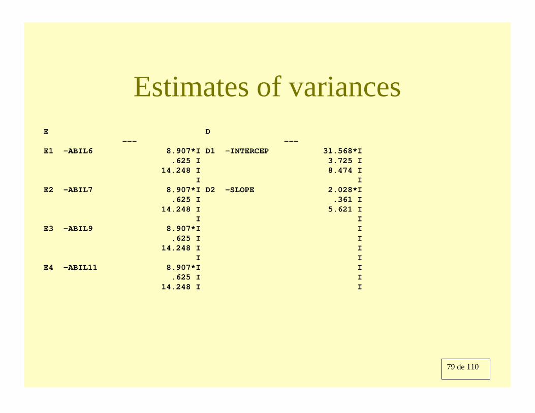
79 de 110

Estimates of variancesE D

--- ---E1 -ABIL6 8.907*I D1 -INTERCEP 31.568*I

.625 I 3.725 I14.248 I 8.474 I

I IE2 -ABIL7 8.907*I D2 -SLOPE 2.028*I

.625 I .361 I14.248 I 5.621 I

I IE3 -ABIL9 8.907*I I

.625 I I14.248 I I

I IE4 -ABIL11 8.907*I I

.625 I I14.248 I I

80 de 110

81 de 110

��

��

Albert SatorraUniversitat Pompeu Fabra. Barcelona

&Juan Carlos Bou

Universitat Jaume I. Castelló

ISI 54TH SESSION, BERLIN, 13-20 AUGUST, 2003

82 de 110

This talk• Introduction: permanent and transitory

components of profits (ROA)• Data & model • Substantive hypotheses• SEM: one- and two-level analyses • Variance decomposition of profits:

– temporary vs permanent– Industry vs firm levels

83 de 110

Introduction• actual profit rates differ widely across firms, both between and within industries.

• Some firms show what can be regarded as ``abnormal returns'', i.e. returns that deviate substantially from the mean return level of all the firms.

• According to economic theory, in a ``competitive market'' these differences should disappear as the time passes.

• How much evidence exists of the persistence of abnormal returns, or how much variation of the returns can be attributed to permanent and time-vanishing components

84 de 110

Data• Initial sample: 5000 Spanish firms

(excluding finance and public companies)• Screened database: 4931 firms• Financial Profit data were collected for each

firm (Return On Assets, ROA)• 6 Time Period: 1995 – 2000• Firms were classified by 4-digit SIC code• Number of Industries: 342 (quasi average

number of firms: 14.28)

85 de 110

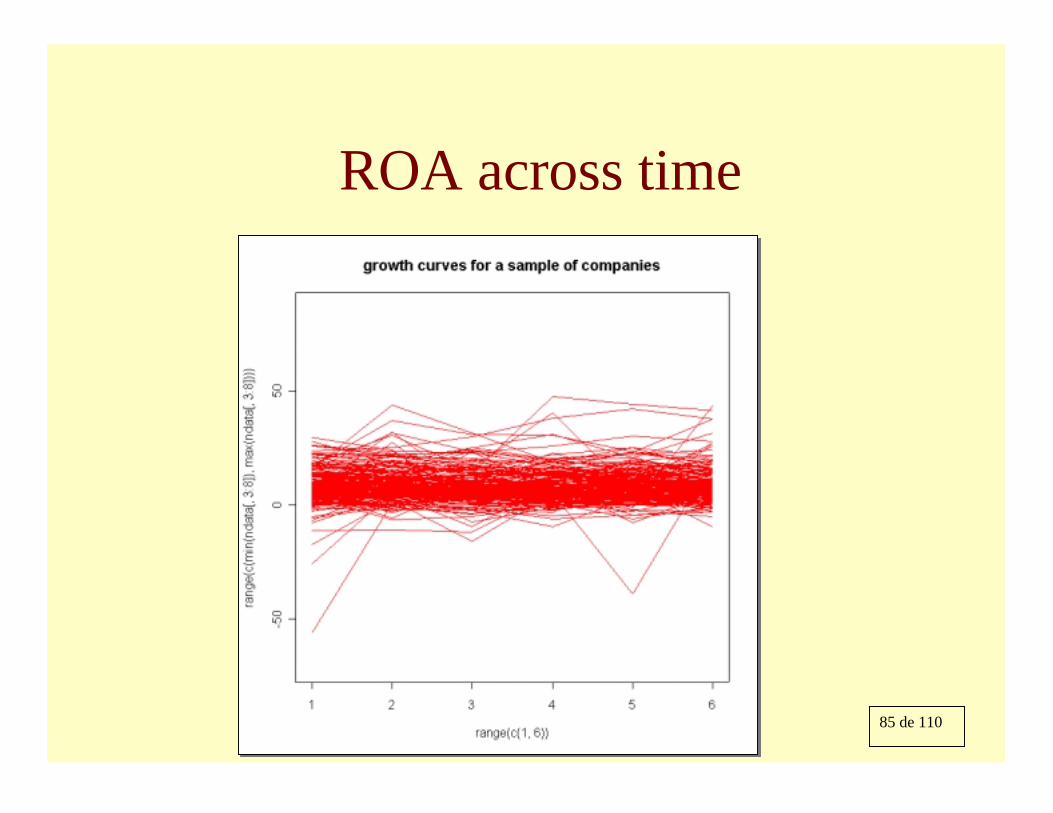
ROA across time

86 de 110

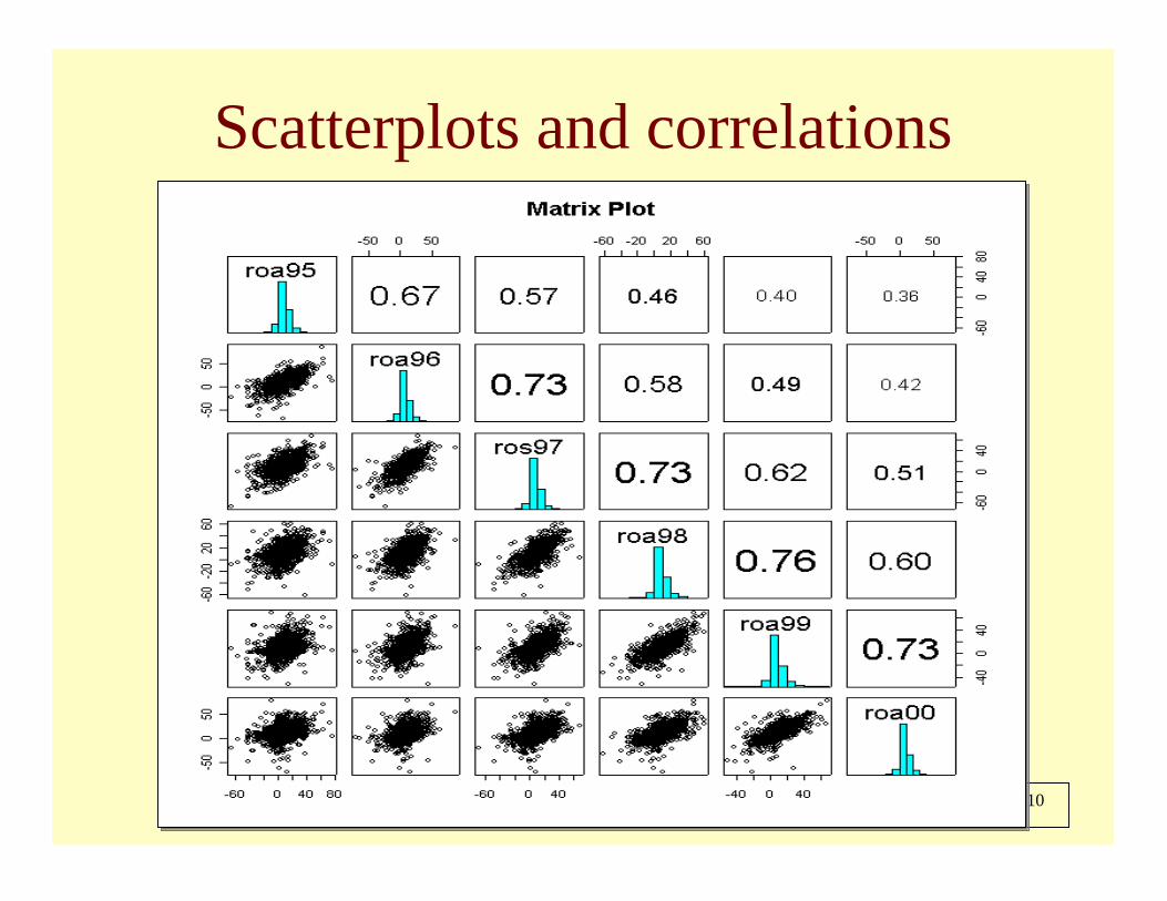
Scatterplots and correlations

87 de 110

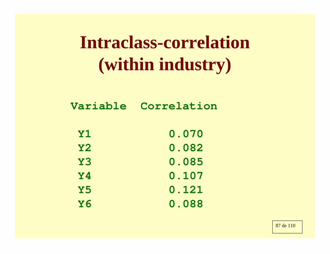
Intraclass-correlation (within industry)

Variable Correlation

Y1 0.070Y2 0.082Y3 0.085Y4 0.107Y5 0.121Y6 0.088

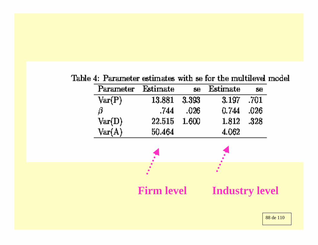
88 de 110

Firm level Industry level

l’anàlisi multivariant aplicada una eina classica i...

Documents