lagrangian relaxation and tabu search approaches for the ... · problem formulation determine which...
TRANSCRIPT

A. Borghetti ^ A. Frangioni * F. Lacalandra ^ A. Lodi §S. Martello § C. A. Nucci ^ A. Trebbi °
§ DEIS, University of Bologna^ Dept. of Electrical Engineering, University of Bologna* Dept. of Computer Science, University of Pisa° Enel Produzione S.p.A
Lagrangian Relaxation andTabu Search Approaches
for the Unit Commitment Problem
Outline of presentation
1. Problem formulation
2. Different computational methods3.1 Lagrangian relaxation3.2 Tabu search
3. Numerical results
4. Conclusions

Problem formulation
Determinewhich electrical power generators to committheir production levelsto supplyforecasted short-term (24 –168 hours) demandspinning reserve requirementsat minimum cost
thermal units: operating cost, history-dependent startup costs, discrete on/off decision, minimum up/down-time, ramping constraints, emission characteristics
( ) ( ) ( ), , , 1 ,, ,1 1min , , min ,
I T
i i t i t i i t i ti t
c u p s u u C−= =
� �� �+ =� �� �
��u p u p
u p
,1
0 1, ,I
t i ti
D p t T=
− = ∀ =� �
min max, , , 1, ,
1, , and constraints
i t i i t i t id ui i
i Iu p p u pt Tτ τ
� ∀ =⋅ ≤ ≤ ⋅ �� ∀ =��
�
�
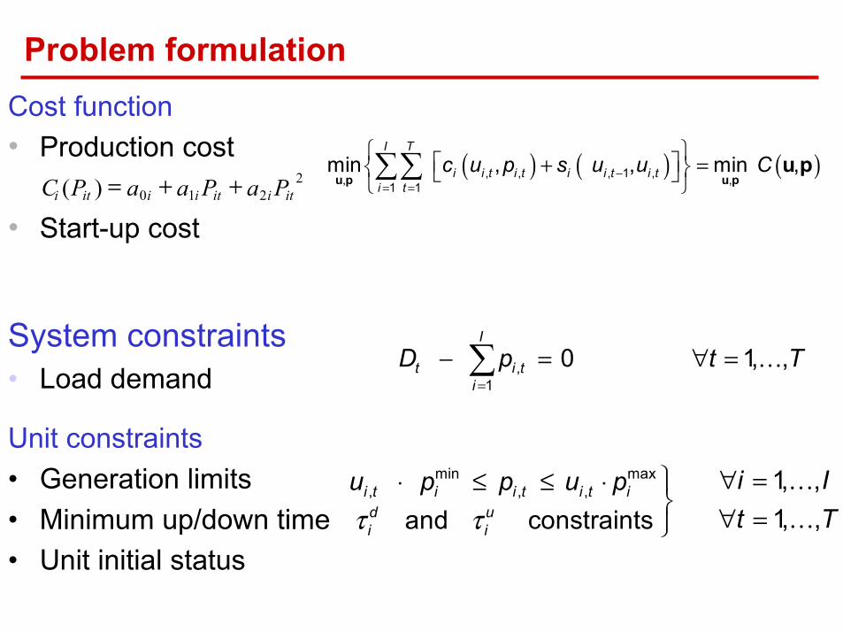
Problem formulationCost function• Production cost
• Start-up cost
2210)( itiitiiiti PaPaaPC ++=
System constraints• Load demand
Unit constraints• Generation limits• Minimum up/down time• Unit initial status
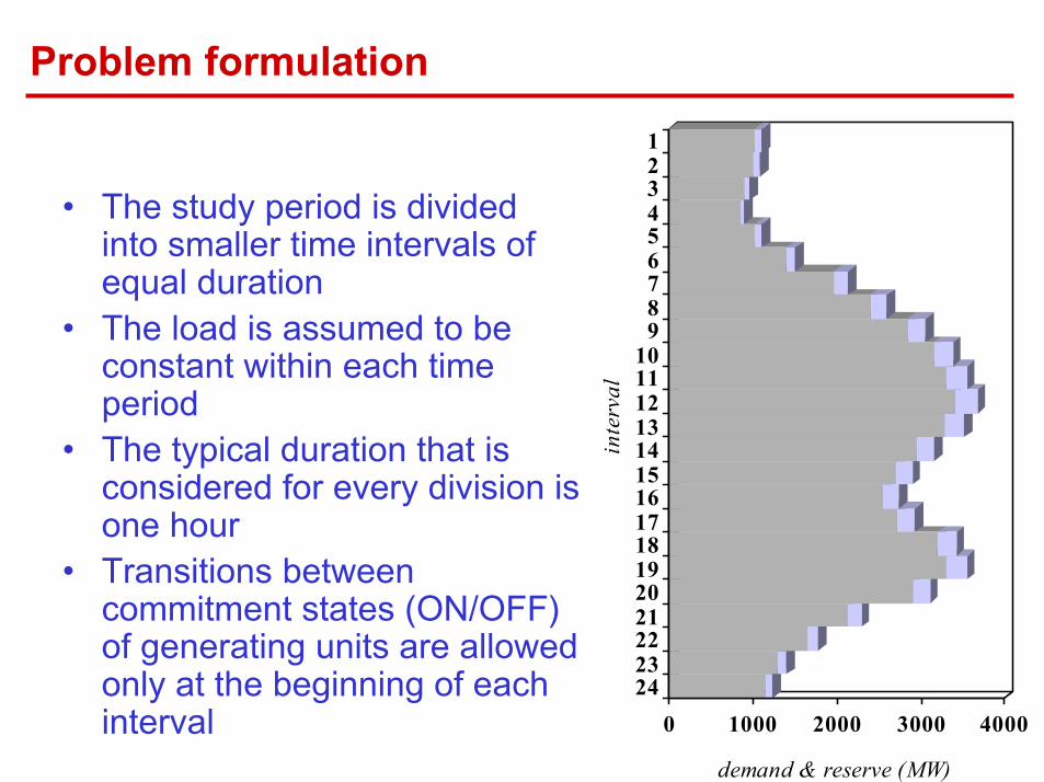
• The study period is divided into smaller time intervals of equal duration
• The load is assumed to be constant within each time period
• The typical duration that is considered for every division is one hour
• Transitions between commitment states (ON/OFF) of generating units are allowed only at the beginning of each interval 0 1000 2000 3000 4000
demand & reserve (MW)
123456789101112131415161718192021222324
inte
rval
Problem formulation
( ) ( ) ,, 1 1min , λ
= =
� �� �= + ⋅ −� �� � � �
� �T I
t t i tt i
L C D pu p
λ u p
Lagrangian relaxation
min max, , , 1, ,
1, , and constraintsτ τ
∀ =�⋅ ≤ ≤ ⋅ �� ∀ =��
�
�
i t i i t i t id ui i
i Iu p p u pt T
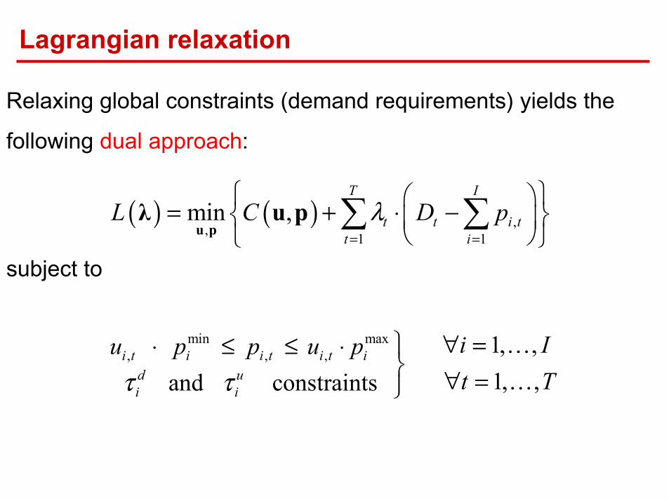
Relaxing global constraints (demand requirements) yields the
following dual approach:
subject to
( ) ( ) ( )1 1
I T
i t ti t
L L Dλ= =
= + ⋅� �λ λ
( ) , , , , 1 ,,1
min , ,( ) ( )λ −=
� �� �� �= − ⋅ +� ��
� � ��
i i
T
i i i t i t t i t i i t i tt
L c u p p s u uu p
λ
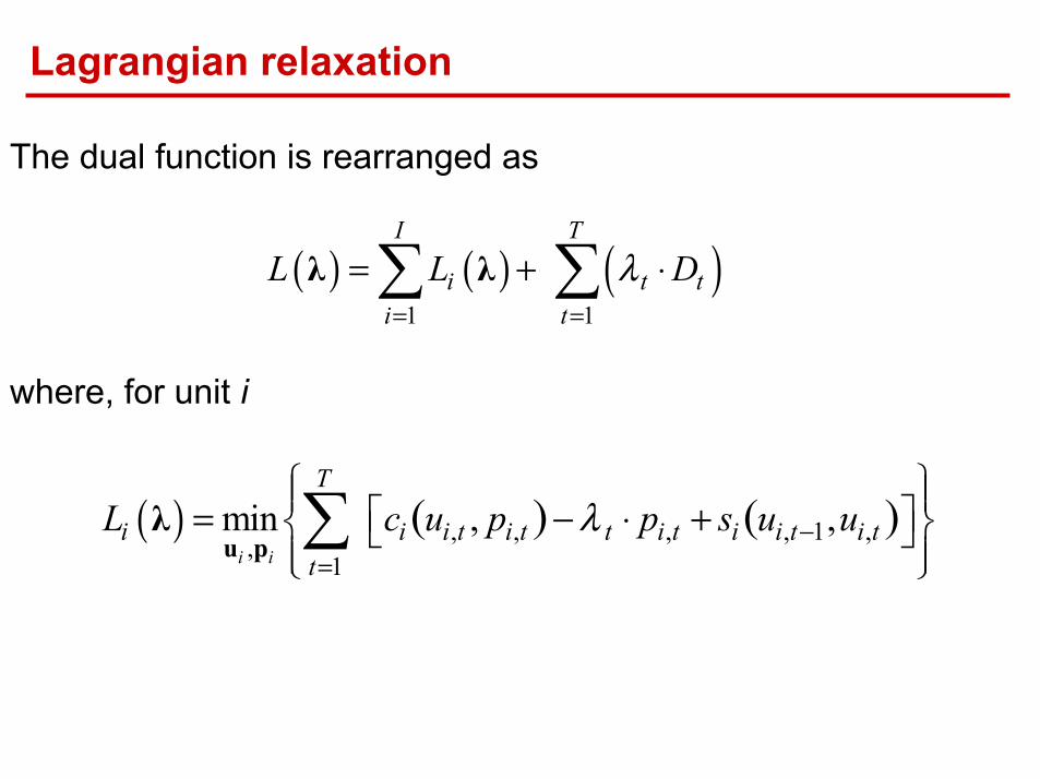
The dual function is rearranged as
where, for unit i
Lagrangian relaxation

( ) , , ,1
min ,( ) λ=
� �� �� �= − ⋅� ��
� � ���
i
T
i i i t i t t i tt
L c u p pp
λ
Lagrangian relaxation
1) Assigned λλλλ and ui , pi is found by solving
Solution in two steps
subject to
min max, , , 1, ,⋅ ≤ ≤ ⋅ ∀ = �i t i i t i t iu p p u p t T
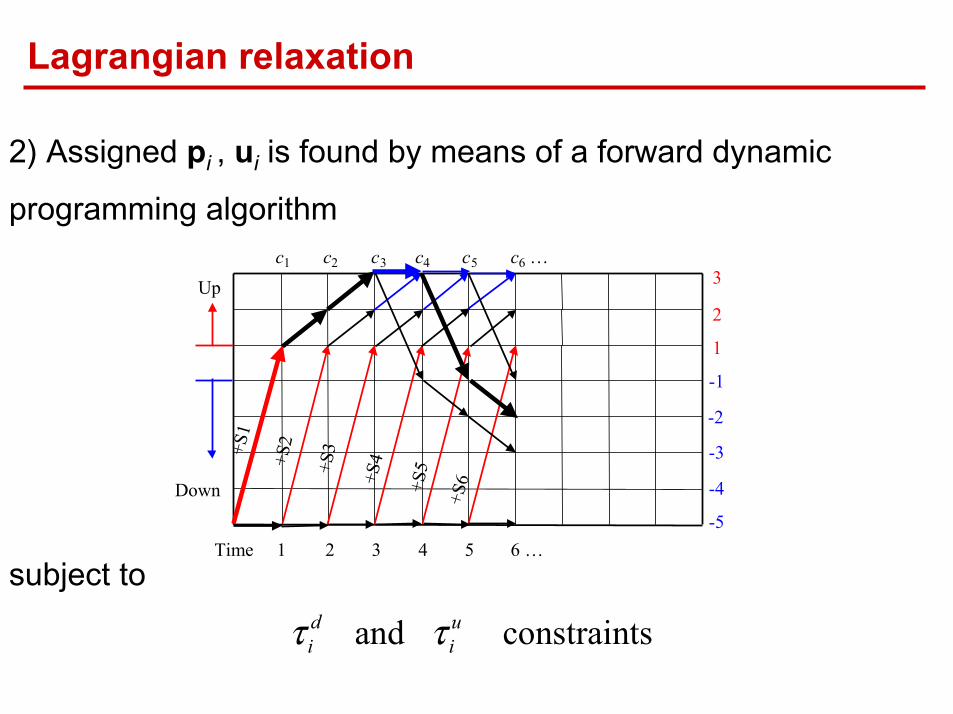
2) Assigned pi , ui is found by means of a forward dynamic
programming algorithm
subject to
and constraintsτ τd ui i
Lagrangian relaxation
Time 1 2 3 4 5 6 …
Up 3
2
1
-1
-2
-3
-4
-5
+S1
+S2
+S3
+S4
+S5
+S6
c1 c2 c3 c4 c5 c6 …
Down

0* max ( )L L
≥=
λλ
Lagrangian relaxation
To find λλλλ, the following dual problem is solved
L* is a lower bound on the optimal objective value of the primal
problem.
Critical points:
1) how to solve the dual problem
2) how to compute a feasible solution

Solve the primal problem(u fixed)
yes
Initialization of multipliers λλλλ
Solve the I de-coupledminimization sub-problems
Evaluate the dual function L(λλλλ)
Is the dual solution feasible?
Heuristic procedure
no
Update multipliers λλλλ
Upper Bound
Lower Bound
until(UB-LB)/LB < spec. value
Lagrangian relaxation
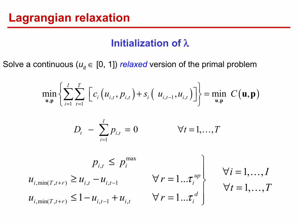
Initialization of λλλλ
Solve a continuous (uit ∈ [0, 1]) relaxed version of the primal problem
( ) ( ) ( ), , , 1 ,, ,1 1min , , min ,−
= =
� �� �+ =� �� �
��
I T
i i t i t i i t i ti t
c u p s u u Cu p u p
u p
,1
0 1, ,=
− = ∀ =� �
I
t i ti
D p t T
max,
,min( , ) , , 1
,min( , ) , 1 ,
1, ,1...
1, ,1 1...
τ
τ+ −
+ −
�≤� ∀ =�≥ − ∀ = � ∀ =�≤ − + ∀ = ��
�
�
i t iup
i T t r i t i t i
di T t r i t i t i
p pi I
u u u rt T
u u u r
Lagrangian relaxation
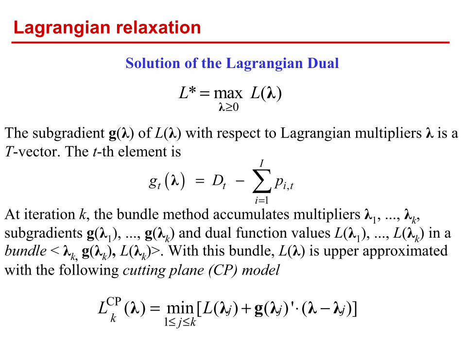
Solution of the Lagrangian Dual
0* max ( )L L
≥=
λλ
CP
1( ) min[ ( ) ( ) ' ( )]j j j
k j kL L
≤ ≤= + ⋅ −λ λ g λ λ λ
( ) ,1
I
t t i ti
g D p=
= − �λ
The subgradient g(λ) of L(λ) with respect to Lagrangian multipliers λ is a T-vector. The t-th element is
At iteration k, the bundle method accumulates multipliers λ1, ..., λk, subgradients g(λ1), ..., g(λk) and dual function values L(λ1), ..., L(λk) in a bundle < λk, g(λk), L(λk)>. With this bundle, L(λ) is upper approximated with the following cutting plane (CP) model
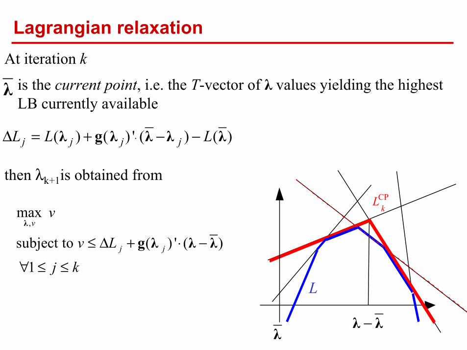
At iteration kis the current point, i.e. the T-vector of λ values yielding the highest LB currently available
λ
( ) ( ) ' ( ) ( )j j j jL L L⋅∆ = + − −λ g λ λ λ λ
then λk+1is obtained from
,max
subject to ( ) ' ( )
1
≤ ∆ + ⋅ −
∀ ≤ ≤
v
j j
v
v Lj k
λ
g λ λ λ
Lagrangian relaxation
CPk
L
L
λ−λ λ
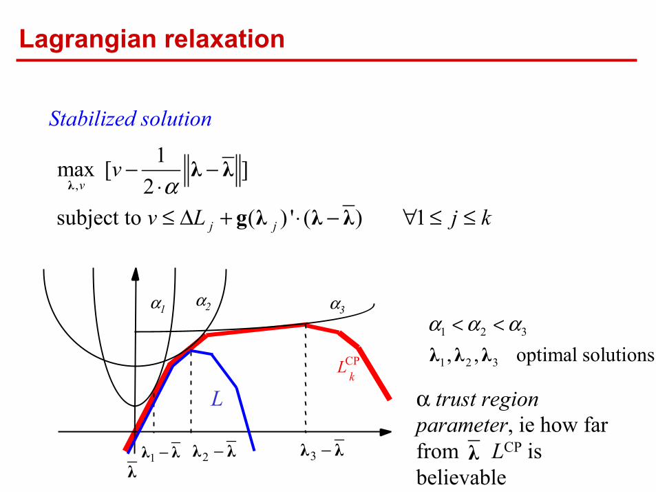
,
1max [ ]2
subject to ( ) ' ( ) 1v
j j
v
v L j kα
− −⋅≤ ∆ + ⋅ − ∀ ≤ ≤
λλ λ
g λ λ λ
Lagrangian relaxation
Stabilized solution
1 2 3
1 2 3, , optimal solutionsα α α< <λ λ λ
α1 α2 α3
3 −λ λ2 −λ λ1 −λ λλ
CPk
L
L α trust region parameter, ie how far from LCP is believable
λ

Bundle disaggregato

Lagrangian relaxation
The Heuristics
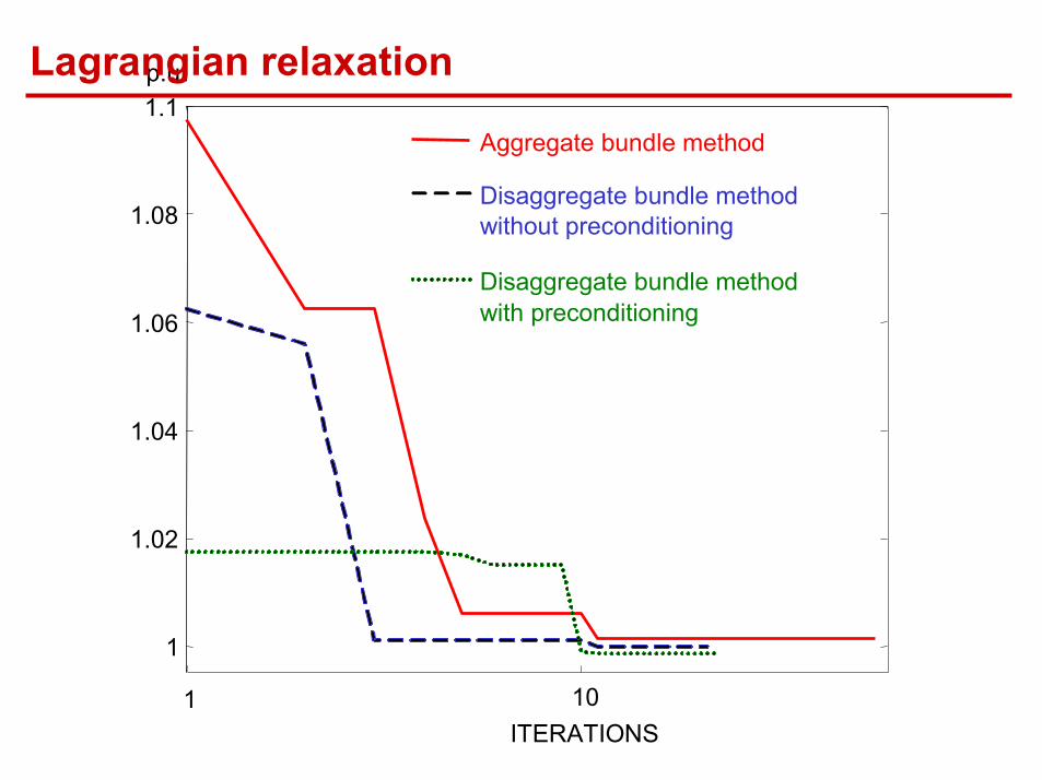
By solving the dual problem by a bundle method, without an extracomputational effort, a “convexified” solution of the original problem is also available. This solution is a matrix with the same dimensions of matrix u, whose elements ui,t∈[0,1] can be interpreted as the “probability” for unit i to be committed at period t.
Making use of this matrix, a heuristic procedure has been implemented trying to uncommit units that are not really needed.
Such a heuristic procedure results in significantly improving the overall performance of the algorithm.

1 10
0.97
0.975
0.98
0.985
0.99
0.995
ITERATIONS
p.u.
Aggregate bundle method
Disaggregate bundle method without preconditioning Disaggregate bundle method with preconditioning
Lagrangian relaxation
1 10
1
1.02
1.04
1.06
1.08
1.1
ITERATIONS
p.u.
Aggregate bundle method
Disaggregate bundle methodwithout preconditioning
Disaggregate bundle methodwith preconditioning
Lagrangian relaxation

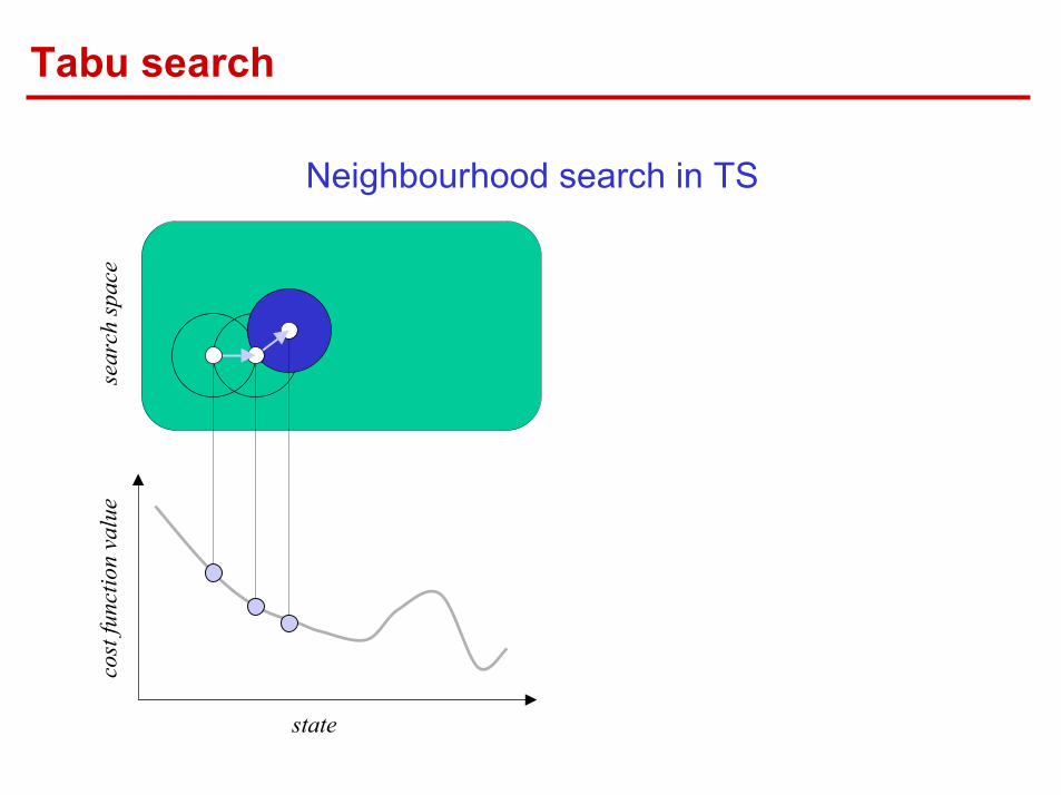
sear
ch sp
ace
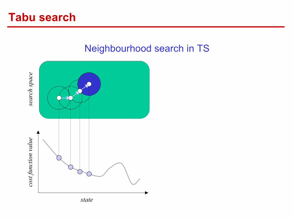
Neighbourhood search in TS
cost
func
tion
valu
e
state
neighbourhood
initial solution
Tabu search

cost
func
tion
valu
e
state
sear
ch sp
ace
Neighbourhood search in TS
Tabu search
cost
func
tion
valu
e
state
sear
ch sp
ace
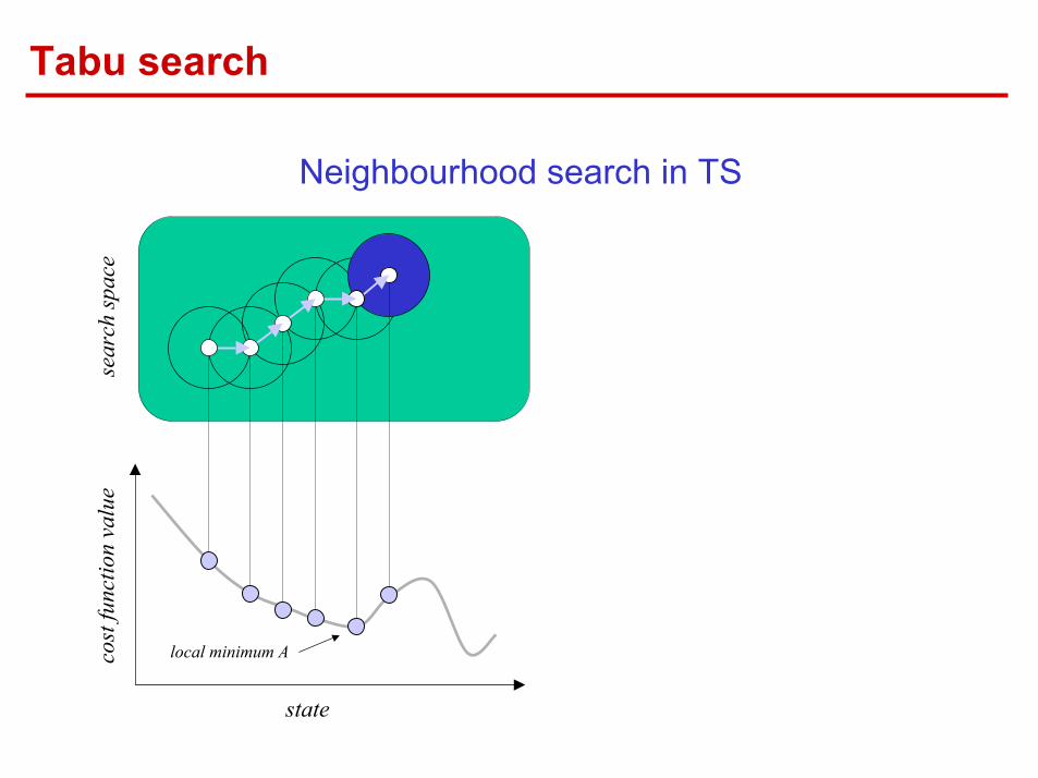
Neighbourhood search in TS
Tabu search
cost
func
tion
valu
e
state
sear
ch sp
ace
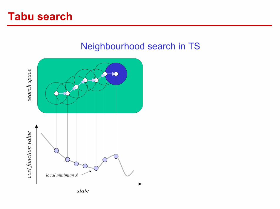
Neighbourhood search in TS
Tabu search

Local search• Partendo da soluzione
iniziale;• generate altre soluzioni;• ottenute una dall’altra
(neighbourhood);• sempre migliori;• termina quando non sono
più possibili miglioramenti.
cost
func
tion
valu
e
state
sear
ch sp
ace
local minimum A
Neighbourhood search in TS
Tabu search
cost
func
tion
valu
e
state
sear
ch sp
ace
local minimum A
Tabu search
Neighbourhood search in TS
cost
func
tion
valu
e
state
sear
ch sp
ace
local minimum A
Tabu search
Neighbourhood search in TS

cost
func
tion
valu
e
state
sear
ch sp
ace
local minimum Blocal minimum A
Tabu Search• Sceglie sempre la soluzione
di costo inferiore;• anche se peggiorante.
Tabu List - TL• Proibisce le mosse più
recenti;• memorizzando alcune
informazioni.
P
Tabu search
Neighbourhood search in TS
Tabu search
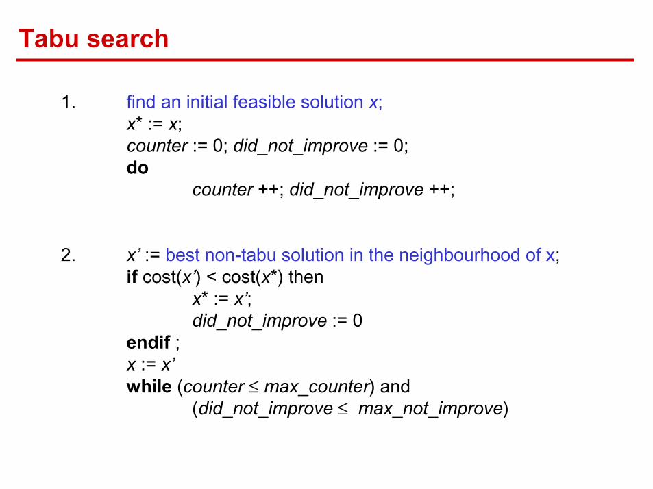
1. find an initial feasible solution x;x* := x;counter := 0; did_not_improve := 0;do
counter ++; did_not_improve ++;
2. x’ := best non-tabu solution in the neighbourhood of x;if cost(x’) < cost(x*) then
x* := x’;did_not_improve := 0
endif ;x := x’while (counter ≤ max_counter) and
(did_not_improve ≤ max_not_improve)
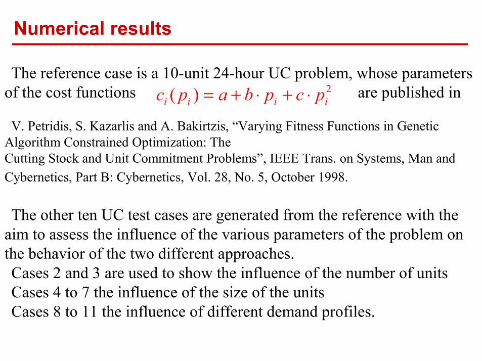
The reference case is a 10-unit 24-hour UC problem, whose parameters of the cost functions are published in
V. Petridis, S. Kazarlis and A. Bakirtzis, “Varying Fitness Functions in Genetic Algorithm Constrained Optimization: TheCutting Stock and Unit Commitment Problems”, IEEE Trans. on Systems, Man and Cybernetics, Part B: Cybernetics, Vol. 28, No. 5, October 1998.
The other ten UC test cases are generated from the reference with the aim to assess the influence of the various parameters of the problem on the behavior of the two different approaches.Cases 2 and 3 are used to show the influence of the number of unitsCases 4 to 7 the influence of the size of the unitsCases 8 to 11 the influence of different demand profiles.
2( )i i i ic p a b p c p= + ⋅ + ⋅
Numerical results
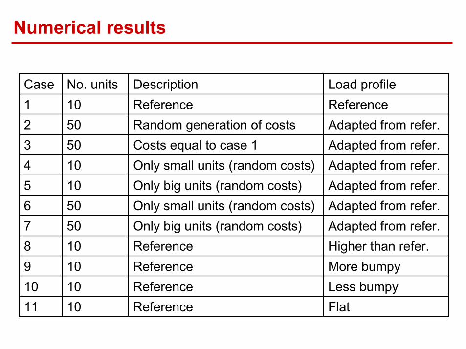
Adapted from refer.Only small units (random costs)506
Flat Reference1011Less bumpyReference1010More bumpyReference109Higher than refer.Reference108Adapted from refer.Only big units (random costs)507
Adapted from refer.Only big units (random costs)105Adapted from refer.Only small units (random costs)104Adapted from refer.Costs equal to case 1503Adapted from refer.Random generation of costs502ReferenceReference101Load profileDescriptionNo. unitsCase
Numerical results

750
850
950
1050
1150
1250
1350
1450
1550
1650
1 2 3 4 5 6 7 8 9 101112131415161718192021222324Time period (h)
Load
(MW
)
Case 1Case 8 - higherCase 9 - more bumpyCase 10 - less bumpyCase 11 - flat
Numerical results

0.717$600,7790.653$600,399$596,503.07110.802$609,6230.711$609,074$604,773.96100.963$616,2140.963$616,216$610,335.590.799$631,9210.761$631,683$626,9137580.231$4,580,8890.124$4,576,011$4,570,335.6570.264$2,010,1080.241$2,009,639$2,004,813.5860.610$943,0190.744$944,275$937,297.5351.113$408,0871.116$408,099$403,593.7040.386$3,048,8130.164$3,042,094$3,037,101.0930.206$3,169,2740.088$3,165,555$3,162,766.7620.548$610,7510.625$611,214$607,420.311
TS Gap (%)Solutionby TS
L R Gap (%)Solutionby L R
Best dual valueCase
Numerical results

$400,000
$900,000
$1,400,000
$1,900,000
$2,400,000
$2,900,000
$3,400,000
$3,900,000
$4,400,000
$4,900,000
1 2 3 4 5 6 7 8 9 10 11
Cases
Solu
tionsLRTSBest dual values
Numerical results
0.0
0.2
0.4
0.6
0.8
1.0
1.2
1 2 3 4 5 6 7 8 9 10 11Cases
Gap
%
LR Gap %TS Gap %
Numerical results
Numerical results
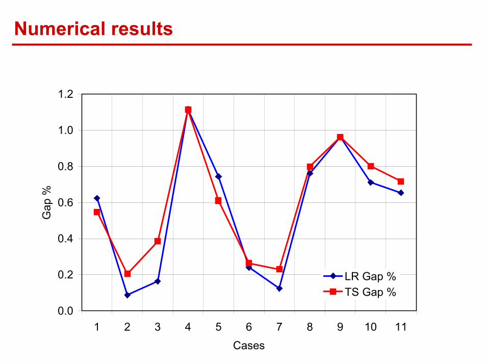
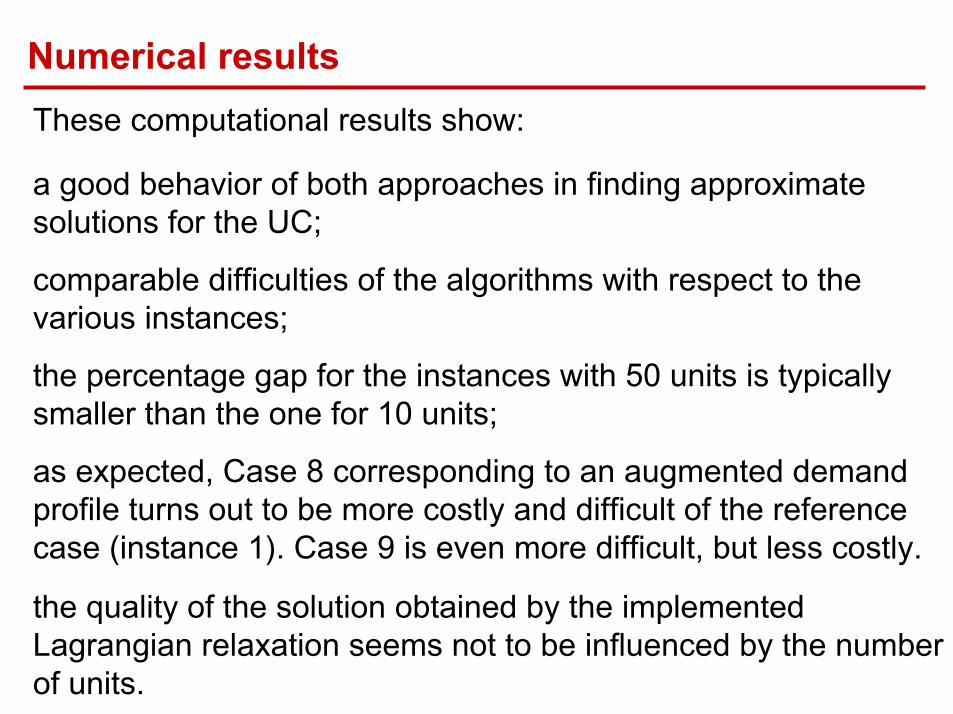
a good behavior of both approaches in finding approximate solutions for the UC;
comparable difficulties of the algorithms with respect to the various instances;
the percentage gap for the instances with 50 units is typically smaller than the one for 10 units;
as expected, Case 8 corresponding to an augmented demand profile turns out to be more costly and difficult of the reference case (instance 1). Case 9 is even more difficult, but less costly.
the quality of the solution obtained by the implemented Lagrangian relaxation seems not to be influenced by the number of units.
These computational results show:
1. In this paper, a Lagrangian relaxation algorithm for the solution of UC problems has been illustrated, wherein the dual problem solution is achieved through the implementation of an improved bundle method and the feasible solution for the primal problem is computed by a heuristic procedure that exploits available hints given by the bundle algorithm. The results obtained by the LR algorithm are compared with those obtained by a Tabu Search algorithm.
2. This comparison has shown a good behaviour of both approaches infinding approximate solutions. Moreover, the analysis of the different and complementary characteristics of the two approaches suggestsfurther research activity to obtain an integrated algorithm of them, able to provide adequate solutions of the new UC problems peculiar of competitive electricity markets.
Conclusions