Lagrangian Coherent Structures (LCS)

CDS 140b - Spring 2012

May 15, 2012ofarrell@cds.caltech.edu

Tuesday, May 15, 12

A time-dependent dynamical system

x(t; t0,x0) = v(x(t; , t0,x0), t)

x(t0; t0,x0) = x0

• • • Assume v is smooth (not necessary, but convenient)

t 2 I ✓ Rx(t; t0,x0) 2 D ✓ Rn

We can define the flow map:

�tt0 : x0 7! �t

t0(x0) = x(t; t0,x0)

as the map which takes a point on the domain at time t0 to its position at time t

Tuesday, May 15, 12

Invariant manifolds in dynamical systems

• If v is independent of t, we can find invariant manifolds• The stable manifolds of a fixed point xc are all the trajectories which asymptote to xc as t ⟶ ∞• The unstable manifolds are all trajectories which asymptote to xc as t ⟶ -∞

Tuesday, May 15, 12

Invariant manifolds in dynamical systems

• If v is independent of t, we can find invariant manifolds• The stable manifolds of a fixed point xc are all the trajectories which asymptote to xc as t ⟶ ∞• The unstable manifolds are all trajectories which asymptote to xc as t ⟶ -∞• Two points on either side of a stable manifold will diverge in forward time• Two points on either side of an unstable manifold will diverge in backward time

Tuesday, May 15, 12

Invariant manifolds in dynamical systems

• If v is independent of t, we can find invariant manifolds• The stable manifolds of a fixed point xc are all the trajectories which asymptote to xc as t ⟶ ∞• The unstable manifolds are all trajectories which asymptote to xc as t ⟶ -∞• Two points on either side of a stable manifold will diverge in forward time• Two points on either side of an unstable manifold will diverge in backward time

Tuesday, May 15, 12

Invariant manifolds in dynamical systems

• If v is independent of t, we can find invariant manifolds• The stable manifolds of a fixed point xc are all the trajectories which asymptote to xc as t ⟶ ∞• The unstable manifolds are all trajectories which asymptote to xc as t ⟶ -∞• Two points on either side of a stable manifold will diverge in forward time• Two points on either side of an unstable manifold will diverge in backward time

Tuesday, May 15, 12

Invariant manifolds in dynamical systems

• If v is independent of t, we can find invariant manifolds• The stable manifolds of a fixed point xc are all the trajectories which asymptote to xc as t ⟶ ∞• The unstable manifolds are all trajectories which asymptote to xc as t ⟶ -∞• Two points on either side of a stable manifold will diverge in forward time• Two points on either side of an unstable manifold will diverge in backward time

Tuesday, May 15, 12

Invariant manifolds in dynamical systems

• If v is independent of t, we can find invariant manifolds• The stable manifolds of a fixed point xc are all the trajectories which asymptote to xc as t ⟶ ∞• The unstable manifolds are all trajectories which asymptote to xc as t ⟶ -∞• Two points on either side of a stable manifold will diverge in forward time• Two points on either side of an unstable manifold will diverge in backward time• Barriers to transport

Tuesday, May 15, 12

Invariant manifolds in dynamical systems

• If v is independent of t, we can find invariant manifolds• The stable manifolds of a fixed point xc are all the trajectories which asymptote to xc as t ⟶ ∞• The unstable manifolds are all trajectories which asymptote to xc as t ⟶ -∞• Two points on either side of a stable manifold will diverge in forward time• Two points on either side of an unstable manifold will diverge in backward time• Barriers to transport• Separatrices between regions of different dynamics

Shawn ShaddenTuesday, May 15, 12

Time-dependent systems

Goal: Find a finite-time approximation to the stable and unstable manifolds, for time-dependent dynamical systems.

• Finite-time: systems often defined in finite time-interval

• Structures that preserve the aforementioned properties, at least in some finite time interval

• Autonomous system:

• Find the fixed points xc

• Linearize about a fixed point

• Find the stable and unstable subspaces

• The stable and unstable manifolds are locally tangent

• Time dependent systems rarely have fixed points

• How do we find LCS? Use the fact that they are separatrices

Finite-Time Lyapunov Exponent (FTLE)

Lagrangian Coherent Structures (LCS)

Tuesday, May 15, 12

The Finite-Time Lyapunov Exponent (FTLE)

• Scalar denoted by

• Measure of how much trajectories starting near a point x at time t diverge over the interval [t, t+T]

• Not an instantaneous separation rate. Measures the integrated separation between trajectories

• In general, the FTLE varies both in space and in time

�Tt (x)

Consider an arbitrary point at t0. When advected by the flow, after time T:

x 2 D

x 7! �t0+Tt0 (x)

Consider a point initially infinitesimally close to x. After a time T the perturbation becomes:

y = x+ �x(t0)

�x(t0 + T ) = �t0+tt0 (y)� �t0+t

t0 (x)

=d�t0+t

t0 (x)

dx�x(t0) +O(||�x(t0)||2)

Tuesday, May 15, 12

The Finite-Time Lyapunov Exponent (FTLE)

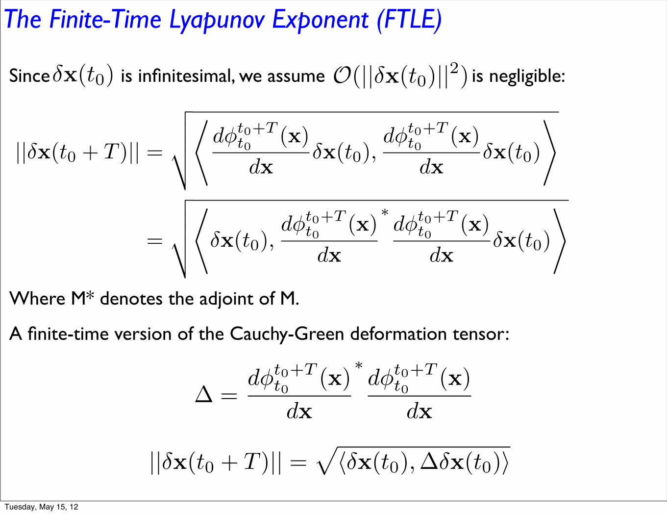
Since is infinitesimal, we assume is negligible:O(||�x(t0)||2)�x(t0)

||�x(t0 + T )|| =

vuut*d�t0+T

t0 (x)

dx�x(t0),

d�t0+Tt0 (x)

dx�x(t0)

+

=

vuut*�x(t0),

d�t0+Tt0 (x)

dx

⇤d�t0+T

t0 (x)

dx�x(t0)

+

Where M* denotes the adjoint of M.

� =d�t0+T

t0 (x)

dx

⇤d�t0+T

t0 (x)

dx

A finite-time version of the Cauchy-Green deformation tensor:

||�x(t0 + T )|| =p

h�x(t0),��x(t0)i

Tuesday, May 15, 12

The Finite-Time Lyapunov Exponent (FTLE)To find the maximum deformation, choose in the direction of the max. eigenvalue of Δ:

�x(t0)

max

�x(t0)||�x(t0 + T )|| =

q⌦�x(t0),�max

(�)�x(t0)↵

=

p�max

(�)||�x(t0)||

Define: �T

t0=

1

|T | lnp

�max

(�)

Then: max

�x(t0)||�x(t0 + T )|| = e�

Tt0

|T |||�x(t0)||

is the FTLE, and it gives a measure of how fast nearby trajectories separate.

Note that the FTLE can be defined equivalently as:

�Tt0

�Tt0 =

1

|T | ln

�����

�����d�t0+T

t0 (x)

dx

�����

�����2

Tuesday, May 15, 12

Computing the FTLE

x1

x2

�t0+Tt0

t0 T

• Compute FTLE field at time t0 on a grid

• Advect particles on the grid by the flow map for a time T

• At each point on the grid:

• Compute the deformation tensor at t0:

• Find the maximum singular value if the deformation tensor.

• Compute T can be positive or negative (integrate trajectories backwards in time)

d�t0+tt0 (x)

dx

�Tt0

Tuesday, May 15, 12

The FTLE field

30

−5 0 5−3

−2

−1

0

1

2

3

✓

�

(a) Velocity field for the simple pendulum.

(b) Repelling FTLE for the simple pendulumflow. The LCS are sharp ridges that separateregions of oscillatory motion from regions of“running” motion.

(c) When combined with the LCS in the at-tracting FTLE field shown here, the LCS fullyenclose the region of oscillatory motion.

Figure 3.1: FTLE and LCS in the flow of the simple pendulum.

Example: pendulum

30

−5 0 5−3

−2

−1

0

1

2

3

✓

�

(a) Velocity field for the simple pendulum.

(b) Repelling FTLE for the simple pendulumflow. The LCS are sharp ridges that separateregions of oscillatory motion from regions of“running” motion.

(c) When combined with the LCS in the at-tracting FTLE field shown here, the LCS fullyenclose the region of oscillatory motion.

Figure 3.1: FTLE and LCS in the flow of the simple pendulum.

✓ ✓

✓

Positive T Negative T

• High values of the positive-time FTLE indicate regions of high particle separation, which coincide with the location of the stable manifolds

• High values of the negative-time FTLE indicate regions of high particle attraction, which coincide with the location of the unstable manifolds

• Combining both FTLE fields, we recover the location of the heteroclinic orbit, which acts as a separatrix between the two dynamically distinct regions

Phil Du Toit

Tuesday, May 15, 12

Lagrangian Coherent Structures are ridges in the FTLE

• Define an LCS as a locally-maximizing curve (ridge) in the FTLE

• A curve is a ridge when:

• A step off the curve in any direction is a step down

• The direction of steepest descent is perpendicular to the ridge

• Define the Hessian of the FTLE:

• A curve c(s) is a ridge if it satisfies:

•

•

where is the smallest eigenvalue of

⌃ =d2�T

t0(x)

dx2

r�Tt0(c(s)) · c

0(s) = 0

�min < 0

�min ⌃

Tuesday, May 15, 12

The time-dependent double-gyreConsider a double-gyre defined by the Stokes streamfunction:

(x, y, t) = A sin(⇡f(x, t)) sin(⇡y)

where:f(x, y) = a(t)x2 + b(t)x

a(t) = ✏ sin(!t)

b(t) = 1� 2✏ sin(!t)

The velocity field: u = �@ @y

; v =@

@x

A = 0.1

! =2⇡

10✏ = 0.25

Shawn ShaddenTuesday, May 15, 12

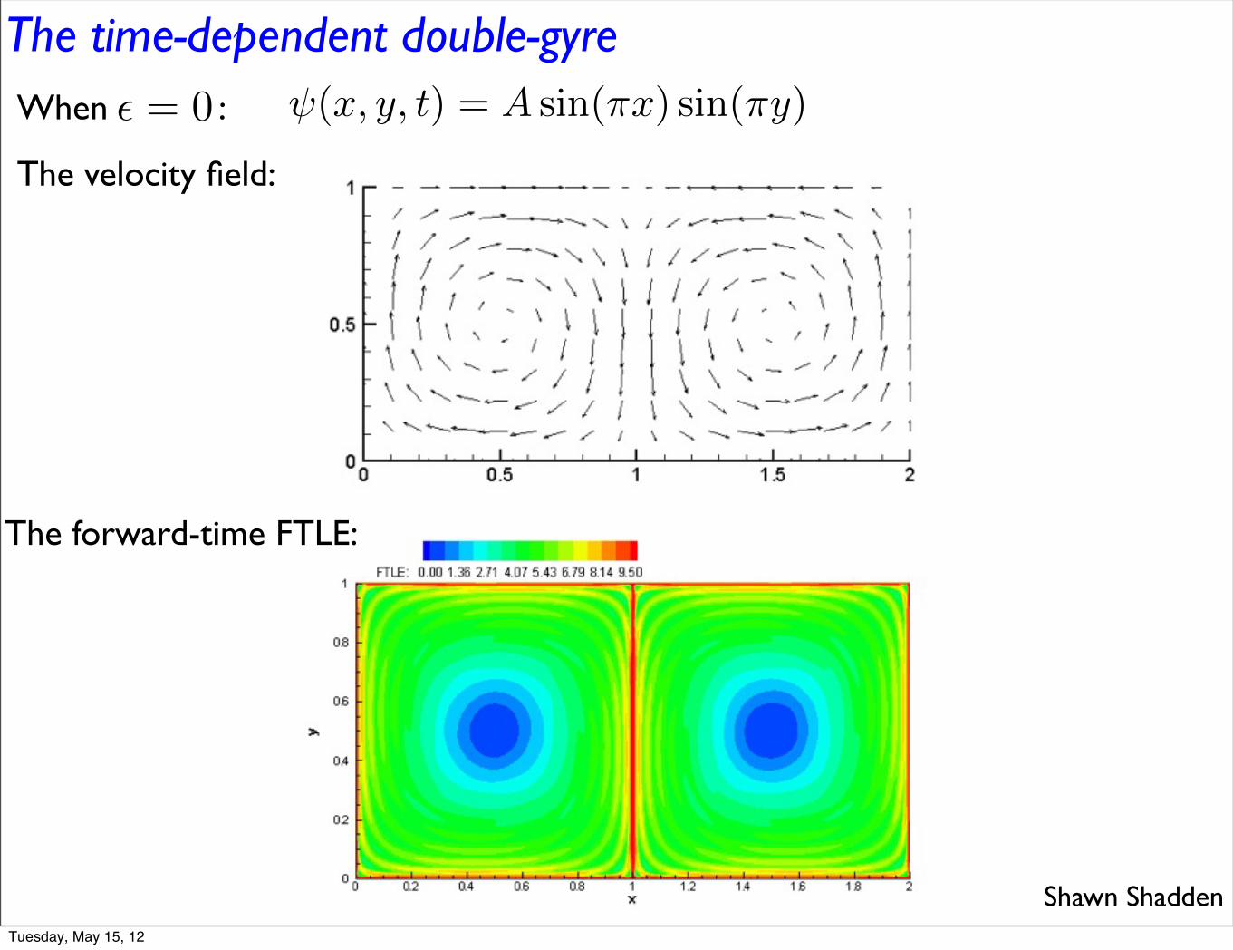
The time-dependent double-gyreWhen :✏ = 0 (x, y, t) = A sin(⇡x) sin(⇡y)

The velocity field:

The forward-time FTLE:

Shawn ShaddenTuesday, May 15, 12

The time-dependent double-gyreWhen :

The forward-time FTLE:

The backward-time FTLE:

Shawn Shadden

✏ 6= 0

Tuesday, May 15, 12

Properties of LCS

• Trajectories that start on an LCS remain on the LCS over the time interval on which it is defined

Shawn Shadden

Tuesday, May 15, 12

Properties of LCS

• Trajectories that start on an LCS remain on the LCS over the time interval on which it is defined• Particles on either side of a repelling LCS diverge away from each other exponentially in forward time

• Particles on either side of an attracting LCS diverge away from each other exponentially in backward time

• Barriers to transport. Flux across a well-defined LCS is, at worst, a slow leak (See Shadden et al 2005 for expression and proof)

• Separatrices between dynamically different regions

Shawn ShaddenTuesday, May 15, 12

Applications of LCS

• ‘Skeleton’ of the flow

73

Figu

re7.3:

Rep

elling

FT

LE

forth

eG

lobal

Ocean

.T

he

LC

Sreveal

bou

ndaries

tom

esoscaleed

dies

that

areresp

onsib

lefor

lateralm

ixing.

Region

sof

intense

activityin

clude

the

Pacifi

cE

quatorial

jets,th

eA

tlanticG

ulf

Stream

,th

eC

ape

Cau

ldron

,an

dth

eA

ntarcticC

ircum

polar

Current.

Phil Du ToitTuesday, May 15, 12

Applications of LCS

• ‘Skeleton’ of the flow

• Transport and mixing

Tuesday, May 15, 12

Applications of LCS

• ‘Skeleton’ of the flow

• Transport and mixing

• Structure identification

Combine forward and backward LCS to find the boundaries of a vortex ring.

Shadden et al 2006.Tuesday, May 15, 12

Applications of LCS

• ‘Skeleton’ of the flow

• Transport and mixing

• Structure identification

• Capture areas

!instantaneous" front and rear stagnation points of the vortexring, as well as its radial extent. It is useful to compare thefidelity of the present LCS methods with quasisteady flowkinematics determined from such an Eulerian analysis.

Figure 10 plots the temporal trend in vortex ring cross-sectional area measured from the previous Euleriananalysis30 along with data measured from the LCS methoddescribed above. The two trends are in close agreement, in-dicating the expected result that the Eulerian and Lagrangiananalyses converge in the limit of steady flow. However, mea-surements from the LCS method tend to be less noisy. Moreimportantly, the LCS method provides much more specificinformation regarding the transport of fluid !e.g., the resultsof the previous section, Sec. IV A 1" and it is not limited byflow unsteadiness as with the Eulerian perspective.

B. Free-swimming Aurelia aurita jellyfish

Figure 11 plots measurements of the velocity field andinstantaneous streamlines generated by a free-swimming Au-relia jellyfish observed from the methods described in Sec.III B. The vortical wake behind the animal is visible andexhibits a flow geometry consistent with previous dyevisualizations.14 However, this Eulerian perspective providesno quantitative indication of the geometry of fluid transport,e.g., the magnitude or distribution of fluid transport betweenthe animal and its surrounding, or the presence of lobedynamics.

FTLE fields were computed from the DPIV data in amanner similar to what was described in Sec. IV A 1 for themechanically generated rings. Figure 12!a" shows the FTLEfield at a given instance in the neighborhood of the jellyfish.

FIG. 11. Panel !a" shows DPIV measurements of the velocity field surround-ing a free-swimming Aurelia jellyfish at an arbitrary time in its swimmingmotion. Panel !b" shows the instantaneous streamlines of the flow in thewake of a jellyfish similar to the one in panel !a".

FIG. 10. Cross-sectional area of the vortex interior as a function of time asmeasured from the streamline method !Ref. 30" and the LCS method de-scribed in Sec. IV.

FIG. 12. !Color online" Panel !a" shows the FTLE field !T=13.3 s, grid spacing of 0.04 cm" at the same time as the measurement in Fig. 11!a". The FTLEfield reveals an LCS, that is superimposed over the jellyfish at a slightly later time in panel !b". The evolution of the LCS indicates which regions of fluid areentrained and shows a recirculation zone behind the jellyfish.

047105-9 Lagrangian analysis of fluid transport in empirical vortex Phys. Fluids 18, 047105 !2006"

Downloaded 11 Apr 2009 to 131.215.6.185. Redistribution subject to AIP license or copyright; see http://pof.aip.org/pof/copyright.jsp

Tuesday, May 15, 12

Applications of LCS

• ‘Skeleton’ of the flow

• Transport and mixing

• Structure identification

• Capture areas

• Flow control

Shawn ShaddenTuesday, May 15, 12

Advantages of LCS

• The FTLE is an integral quantity, so it is robust to noise in the velocity data (Haller 2002). Useful for experimental results.

• Unambiguous: not sensitive to threshold value.

• Frame invariant.

Shawn ShaddenTuesday, May 15, 12

Disadvantages of LCS

• Requires time-resolved velocity data.

• FTLE field returns a wealth of information about particle trajectories, but it is sometimes difficult to interpret, and not useful in every application.

• For every time step t you want the the FTLE for:

• Initialize particles on a rectangular grid at time t

• Advect trajectories forward for the integration time T using a Runge-Kutta scheme

• Find the final particle positions at time t+T

• Compute the FTLE field

EXTREMELY EXPENSIVE!

Tuesday, May 15, 12

The speed issue

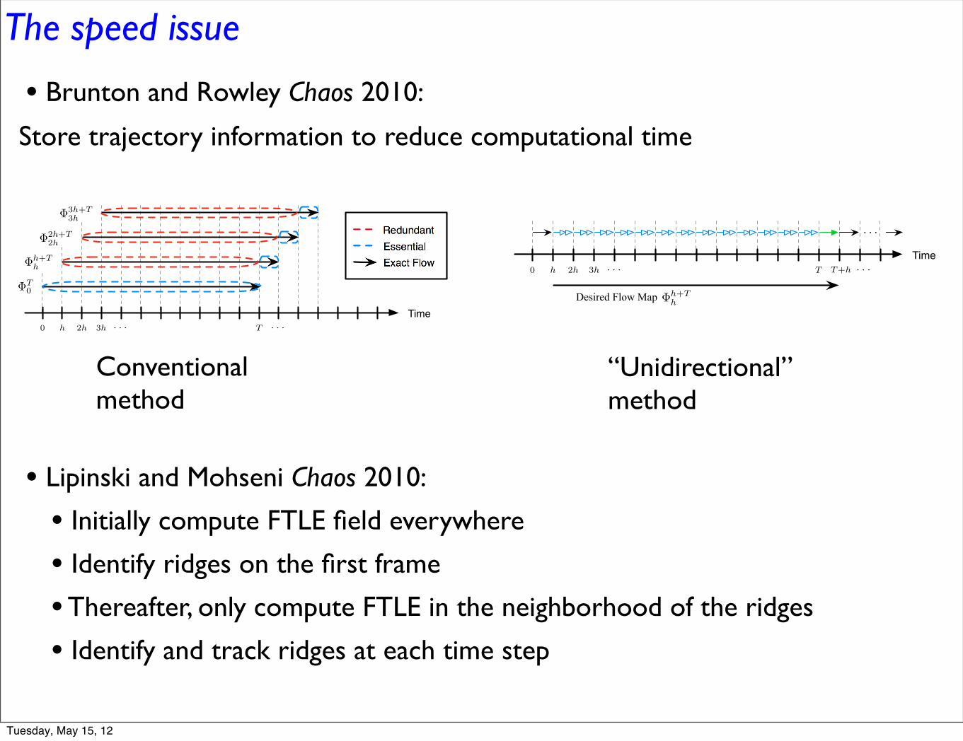
• Brunton and Rowley Chaos 2010:

• Lipinski and Mohseni Chaos 2010:

• Initially compute FTLE field everywhere

• Identify ridges on the first frame

• Thereafter, only compute FTLE in the neighborhood of the ridges

• Identify and track ridges at each time step

2

over the standard method, and computational improve-ment scales with the desired time resolution of the FTLEanimation.

The bidirectional method su↵ers from significant er-ror which is aligned with the opposite-time Lagrangiancoherent structures. To understand this coherent error,we provide an error analysis for both methods, and un-cover an important relationship between positive-timeLCS (pLCS) and negative-time LCS (nLCS). In particu-lar, in the neighborhood of a time-dependent saddle, par-ticles near the pLCS flow into particles near the nLCS inpositive time.

II. STANDARD COMPUTATION OF FTLE

Consider a time-dependent velocity field u on Rn anda particle trajectory x(t) which satisfies

x = u (x(t), t) . (1)

The velocity field, u, may be an unsteady solution of theNavier-Stokes equation, although it is only assumed thatu is at least C

0 in time and C

1 in space. However, to ex-tract Lagrangian coherent structures from the Hessian ofthe FTLE field, u must be C

2 in space [4]. The velocityfield may be analytically defined, but is more often ob-tained from experiments or direct numerical simulationwhich produce velocity field data at discrete snapshotsover a finite range of time. A method of computing finite-time Lyapunov exponents (FTLE) on a finite amount ofdiscrete velocity field data has been developed [3, 4].

Computing an FTLE field typically involves four steps.First, a grid of particles X

0

⇢ Rn is initialized over thedomain of interest. The particles are advected (i.e., inte-grated) with the flow from initial time 0 to final time T ,resulting in a time-T particle flow map, �T

0

, defined as:

�T0

: Rn ! Rn; x(0) 7! x(0) +Z T

0

u(x(⌧), ⌧)d⌧. (2)

Next, the flow map Jacobian, D�T0

is computed, usu-ally by finite-di↵erencing, to obtain the Cauchy-Greendeformation tensor,

� =�D�T

0

�⇤D�T

0

(3)

where ⇤ denotes transpose. Finally, the largest eigen-value, �

max

, of this symmetric tensor is extracted andsynthesized into an FTLE field:

�(�T0

;x) =1

|T | logp

�

max

(�(x)). (4)

The bottleneck in this procedure is the large number ofparticle integrations required to obtain the particle flowmap, �T

0

. Moreover, if the velocity field is time-varying,it is necessary to compute a sequence of FTLE fields intime to visualize unsteady events, as shown schematicallyin Fig. 1.

�T0

�h+Th

�2h+T2h

�3h+T3h

3h2hh0 T . . .. . .

FIG. 1: The standard method for computing FTLE fields.Flow maps �kh+T

kh for k 2 {0, 1, 2, 3} are shown (solid blackarrow). Essential (blue) and redundant (red) particle integra-tions are outlined in dashed ovals.

III. FLOW MAP APPROXIMATION

As seen in Fig. 1, the standard method of computing asequence of FTLE fields involves ine�cient re-integrationof particles. The unidirectional and bidirectional meth-ods outlined below streamline the computation of neigh-boring FTLE fields by approximating the time-T flowmap, �t0+T

t0 , which can be written as:

�t0+Tt0 = �tN

tN�1� · · · � �t2

t1 � �t1t0 (5)

where tN = t

0

+ T .Because the flow maps are obtained numerically on

a discrete grid of points, X

0

⇢ Rn, it is necessary tointerpolate the maps at points x /2 X

0

. Consider a flowmap � : Rn ! Rn, and the same flow map restricted toX

0

, �|X0 : X

0

! Rn. The interpolation operator I takesthe discrete map �|X0 and returns the interpolated map,I� : Rn ! Rn, which approximates � on Rn:

I : �|X0 7! I�. (6)

Here we use the shorthand I� , I (�|X0). We nowobtain an approximation to the flow map in Eq. (5):

�t0+Tt0 (X

0

) = I�tNtN�1

� · · · � I�t2t1 � �t1

t0(X0

)

⇡ �t0+Tt0 (X

0

)(7)

The bidirectional method approximates the time-T flowmap �t0+T

t0 by first integrating backward to a referencetime, t = 0, then interpolating forward through a previ-ously computed time-T map, �T

0

, and finally integratingforward to time t

0

+ T . The unidirectional method ap-proximates the time-T flow map by composing a num-ber of smaller time flow maps, �ti+h

ti, which all have the

same time direction. Additionally, the chain rule may beapplied to each of the methods, resulting in an approxi-mation to the flow map Jacobian, D�t0+T

t0 .

A. Bidirectional Composition

Bidirectional approximation eliminates redundancyfrom neighboring FTLE field computations by using the

3

information from a known flow map at a given time, �T0

,to calculate an approximation to the flow map at futuretimes, �t0+T

t0 . First, X

0

is integrated backward from t

0

tothe reference time 0. The distorted grid �0

t0(X0

) is thenflowed forward through the interpolated map, I�T

0

, andfinally integrated forward an amount t

0

to the desiredtime t

0

+ T , as in Fig. 2:

�t0+Tt0 = �t0+T

T � I�T0

� �0

t0 . (8)

3h2hh0 . . .. . . T

�T0

FIG. 2: Schematic for bidirectional method (a). Given aknown flow map �T

0 (solid black arrow), it is possible to ap-proximate the flow map at later times �kh+T

kh (dashed blackarrow) by integrating backward in time to t = 0 (red arrow),flowing forward through the interpolated map I�T

0 which wasalready computed (blue double arrow), and integrating tra-jectories forward to the correct final time (green arrow).

The flow �T0

is stored as a reference solution to com-pute an approximation to the flow map at later times�kh+T

kh ⇡ �kh+Tkh by

�kh+Tkh = �kh+T

T � I�T0

� �0

kh k 2 Z (9)

Instead of using �T0

as the reference solution for everyfuture time, it is convenient to use the new approximateflow map �h+T

h as the reference solution for the nextiteration:

�2h+T2h = �2h+T

h+T � I�h+Th � �h

2h (10)

This method may be continued, using �kh+Tkh to approx-

imate �(k+1)h+T(k+1)h :

�(k+1)h+T(k+1)h = �(k+1)h+T

kh+T � I�kh+Tkh � �kh

(k+1)h. (11)

Errors will compound more quickly since approximateflow maps as used as the reference solutions for later ap-proximations, as seen in Fig. 3.

B. Unidirectional Composition

The basis of the unidirectional method is to eliminateredundant particle integrations by only integrating par-ticle trajectories through a given velocity field a single

3h2hh0 . . .. . . T

�T0

FIG. 3: Schematic for bidirectional method (b). As in Fig. 2,a known flow map (solid black arrow) is used to approximatethe flow map at a later time �kh+T

kh (dashed black arrow).The approximate flow map is used as the known map for thenext step (dashed black arrow).

time. If a sequence of FTLE snapshots is desired at atime spacing of h, for example as frames in an anima-tion, then it is convenient to break up the time-T flowmap into smaller time-h flow maps, where T = kh:

�kh0

= I�kh(k�1)h � · · · � I�2h

h � �h0

(12)

This method is called unidirectional because particle flowmaps of the same time direction are used, as opposed tothe bidirectional method which composes both positive-time and negative-time flow maps.

. . .

3h2hh0 . . .. . . T+hT

�h+Th

FIG. 4: Schematic for unidirectional method. Time-h flowmaps (short blue arrows) are stored and composed to ap-proximate the time-T flow map (long black arrow). The nextflow map only requires integrating one new time-h flow map(green arrow).

The simplest approach is to compute a number of time-h flow maps and store them in memory. Then, to con-struct an approximate �t0+T

t0 , it remains only to composethe sequence of interpolated time-h flow maps. The nextiteration involves integrating one more time-h flow mapand composing the next sequence, as in Fig. 4.

To further improve e�ciency by reducing the totalnumber of flow map compositions, it is possible to con-struct a multi-tiered hierarchy of flow maps for reuse inneighboring flow map constructions. With enough mem-ory, it is possible to reduce the number of interpolatedcompositions by increasing the number of tiers of flowmaps, each tier being constructed as the composition oftwo of the flow maps in the next tier lower, as in Fig. 5.

Conventional method

“Unidirectional” method

Store trajectory information to reduce computational time

Tuesday, May 15, 12

Resources and references

• Shawn Shadden’s LCS tutorial: http://mmae.iit.edu/shadden/LCS-tutorial/contents.html

• Phil Du Toit’s CDS thesis:http://thesis.library.caltech.edu/5293/

Software

Introduction to LCS

• Jeff Peng’s LCS Matlab kit: http://dabiri.caltech.edu/software.html

• Francois Lekien’s MANGEN:http://mmae.iit.edu/shadden/LCS-tutorial/mangen.html

• Phil Du Toit’s Newman:(No longer available online. Contact me at ofarrell@)

Journal articles

• G. Haller, Chaos 10:99-108 (2000)• G. Haller and G. Yuan, Physica D 147:352-70 (2000)• G. Haller, Phys. Fluids A 14:1851-61 (2002)• Mathur et al, Phys. Rev. Lett. 98:144502 (2007) • Shadden et al, Physica D 212:271-304 (2005)

Tuesday, May 15, 12

Project suggestions

• FTLE computation and testing in classical flows

• LCS computation using open source software

• G. Haller and T. Sapsis, “Lagrangian coherent structures and the smallest finite-time Lyapunov exponent.” Chaos 21 (2011)

• Hyperbolicity in LCS

• Mathur et al 2007

• Green et al, Journal of Fluid Mechanics 572:111 (2007)

In the press

• “Finding order in the apparent chaos of currents,” The New York Times, 28 September 2009• “The skeleton of water, ” The Economist, 12 November 2009

Tuesday, May 15, 12