UCRL-JC-132657 Preprint

Laboratory Scale Tests of Electrical Impedance Tomography

A. Ramirez, W. Daily, A. Binley and D. LaBrecque

This paper was prepared for submittal to Symposium of the Application of Geophysics to

Engineering and Environmental Problems Oakland, California

March 14-18,1999

December 1,1998

This is a preprint of a paper intended for publication in a journal or proceedin Since changes may be made before publication, this preprint is made available with the understanding that it will not be cited or reproduced without the permission of the author.

DISCLAIMER

This document was prepared as an account of work sponsored by an agency of the United States Government. Neither the United States Government nor the Universitv of California nor any of their employees, makes any warranty, express or implied, or assumes any legal liability or responsibility for the accuracy, completeness, or usefulness of any information, apparatus, product, or process disclosed, or represents that its use would not infringe privately owned rights. Reference herein to any specific commercial product, process, or service by trade name, trademark, manufacturer, or otherwise, does not necessarily constitute or imply its endorsement, recommendation, or favoring by the United States Government or the University of California. The views and opinions of authors expressed herein do not necessarily state or reflect those of the United States Government or the University of California, and shall not be used for advertising or product endorsement purposes.

LABORATORY SCALE TESTS OF ELECTRICAL IMPEDANCE TOMOGRAPHY

Abelardo Ramirez* W illiam Daily*

Andrew Binley** Douglas LaBrecque***

*Lawrence Livermore National Laboratory, Livermore CA **Lancaster University, Lancaster, UK

***Steamtech, Inc., Bakersfield, CA

ABSTRACT Electrical impedance tomographs (magnitude and phase) of known, laboratory-scale targets are reported. Three methods are used to invert electrical impedance data and their tomographs compared. The first method uses an electrical resistance tomography (ERT) algonthm (designed for DC resistivity inversion) to perform impedance magnitude inversion and a linearized perturbation approach (PA) to invert the imaginary part. The second approximate method compares ERT magnitude inversions at two frequencies and uses the frequency effect (FE) to compute phase tomographs. The third approach, electrrcal impedance tomography (EIT), employs fully complex algebra to account for the real and imaginary components of electrical impedance data. The EIT approach provided useful magnitude and phase images for the frequency range of 0.0625 to 64 Hz; images for higher frequencies were not reliable. Comparisons of the ‘ERT and EIT magnitude images show that both methods provided equivalent results for the water blank, copper rod and PVC rod targets. The EIT magnitude images showed better spatial resolutron for a sand-lead mixture target. Phase images located anomalies of both high and low contrast IP and provided better spatial resolution than the magnitude images. When IP was absent from the data, the EIT algorithm reconstructed phase values consistent with the data noise levels.

INTRODUCTION Electrical resistance tomography (ERT) was proposed independently by Henderson and Webster (1978) as a medical imaging tool and by Lytle and Dines (1978) as a geophysical imaging tool. The technique has been actively developed for medical imaging (e.g., Isaacson, 1986; Barber and Seager,1987; Yorkey et al., 1987). Early adaptations of the technique to the field of geophysics were by Pelton et al., (1978), Dines and Lytle (1981), Tripp et al. (1984), Wexler et al., (1985), Oldenburg and Li (1994), Sasaki (1992), and Daily and Owen (1991).

Published efforts to image both the magnitude and phase of the measured impedance (BIT) have been relatively few. Many have relied on a linear approximation such as that by Seigel (1959) which requires a knowledge of the DC resistivity distribution (also Oldenburg and Li, 1994). Recent algorithms which also solve the EIT inversion problem can be found in Weller et al. (1996), Yuval and Oldenburg (1997) and in Shi et al. (1998).

The purposes of the work presented here are to: 1) evaluate a rigorous electrical impedance (EIT) algorithm which solves the forward and inverse problems using complex algebra to account for both the resistive and reactive nature of the current flow and 2) compare results from this rigorous method to results obtained from approximate

1

methods. Laboratory-scale targets having known location, size, and IP response were used to provide data for these evaluations.

ELECTRICAL IMPEDANCE INVERSION The goal is to calculate the impedance distribution which is consistent with impedance magnitude and phase measurements made on the boundary of a region. To formulate the forward problem, we assume that the region of interest may be represented as a two- dimensional impedance distribution p *. If electromagnetic effects can be neglected, the forward problem is defined by the Fourier transformed Poisson’s equation for a point source with real current

Herev *is the transformed complex potential and h is the transformation variable. This differential equation may be solved using the finite element method for given boundary conditions. Inverse Fourier transform and appropriate superposition of the calculated potentials yields the complex transfer resistance of an arbitrary electrode configuration in the plane, from which an apparent conductivity can be calculated.

To solve the inverse problem, due to a possibly wide range of impedances, it is common to use log transformed parameters, that is, Pj* = -ln(rj*) (j=1,2,. . .,M) as the parameters of the inversion, where pj* are the complex resistivities of one or more elements depending on the parametrization and M is the number of parameters. Note that the complex logarithm separates the real logarithm of magnitude and phase of its argument into real and imaginary parts.

The objective function minimized here consists of the data misfit (with F as the operator of the forward solution, as before) and the model roughness (as used for numerous ERT inversion algorithms, see for example equations (8) and (9)):

~@*)=[D*-F*(P*)]WTFqD*-F*(P*)]+fxP*TRP* (2) where D* are the measured complex resistances, and as before, F*(P*) are the corresponding forward model resistances due to parameters P*, W is a vector of standard deviations of the data used to weight individual measurements, R is a roughness matrix used to force smoothing of the resistivity distribution and stabilize the inverse solution and a is the smoothing parameter.

Minimization of the objective function in (2) is achieved through an iterative solution. The procedure terminates when the desired data misfit has been reached. The approach is similar to that originally employed by deGroot-Hedlin and Constable (1990). The objective function in the form of equation (2) is real even though the data, model and parameters are complex terms. This formulation imposes restrictions on assignment of complex weights, because the product WW is also real. Consequently, it is impossible to separate errors in magnitude and phase in the weighting process. This could be achieved by decoupling the real and imaginary components; this approach may be the logical

2

extension of this work. Our objective here, however, is to explore the possible benefits (if any) of a fully complex inversion of EIT data in comparison to more conventional procedures such as PA and PFE.

APPROXIMATE METHODS The first method uses an ERT algorithm designed for DC resistivity inversion (Oldenberg and Li, 1994; Zhang et al., 1995; LaBrecque et al., 1996) to perform the impedance magnitude inversions, and a linearized perturbation approach (PA, as described in Oldenberg and Li, 1994) to invert the imaginary part. The second approximate method computes the phase tomographs by comparing two ERT magnitude inversions at two frequencies, and then uses the frequency effect (FE, as described in Pelton et al., 1978) to compute phase tomographs.

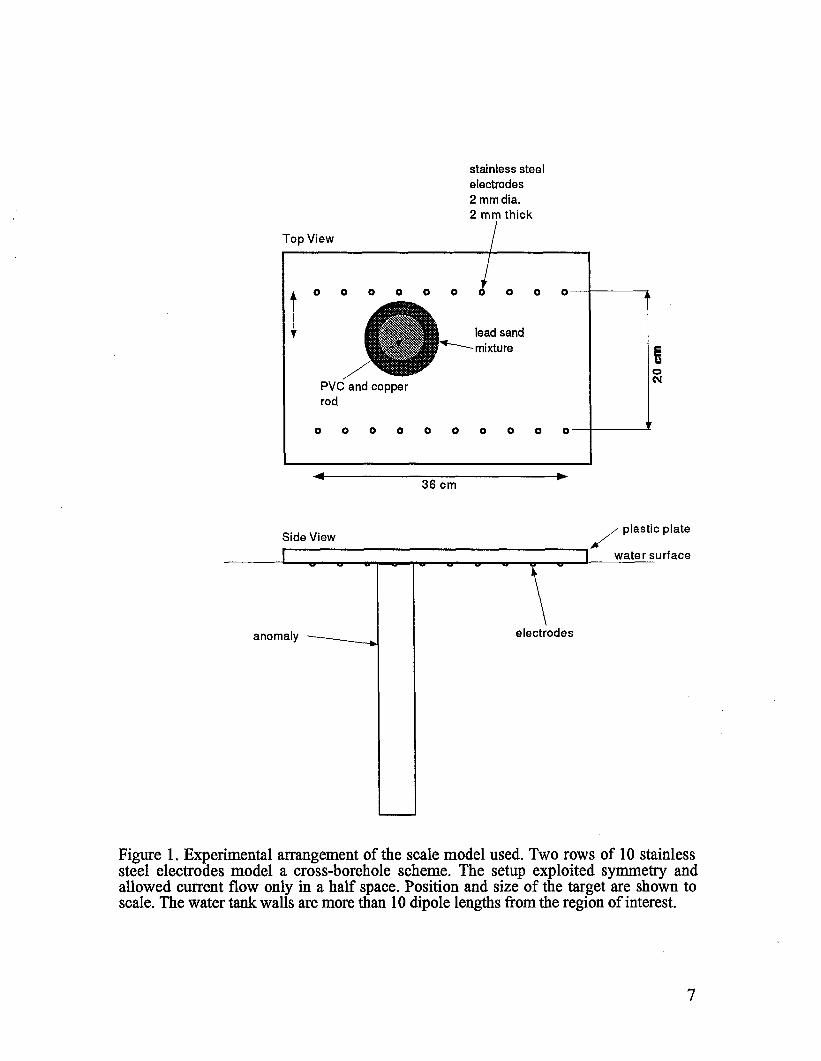
EXPERIMENTAL PROCEDURE The physical scale model we used to generate test data reproduced the sampling geometry typical of geophysical electrical imaging. Twenty electrodes were arranged, as shown in Figure 1, in two columns of 10 to simulate the arrangement typical of cross borehole imaging. The electrode arrays were mounted on one side of a plastic plate which was placed horizontally at the surface of the water. Anomalies were attached to the plastic plate to hang between the electrode arrays in the uniformly conductive water. The fiberglass water tank was 3.1 meters in diameter and 2.45 meters deep; large relative to the electrode array dimensions to eliminate significant effects in the measurements from the tank walls.

Each data set consisted of 170 linearly independent measurements (plus a full set of reciprocal measurements). A dipole-dipole survey approach was used to collect the data. The ratio of each voltage to the corresponding current is a (complex) transfer impedance consisting of a magnitude and phase. Data were acquired at 8 frequencies: 0.0625, 0.25, 1 .O, 4.0, 16, 64, 256 and 1024 Hz on each of 4 resistivity scale models. Four resistivity models used were:

Model 1. No target present; this model will be referred to as the “water. blank” model. Water of uniform resistivity was the target.

Model 2. Metallic target; this model will be referred to as the “copper rod” model. A 6.7 cm diameter PVC pipe wrapped with copper tape was placed in the water with its long axis perpendicular to the plane of the electrodes.

Model 3. Plastic target; this model will be referred to as the “PVC rod” model. A 6.7 cm diameter PVC pipe was placed in the water below the image plane with its long axis perpendicular to the plane of electrodes.

Model 4. Intermediate contrast target; this model will be called the “sand-lead ” model. A cloth bag containing a mixture of sand and lead shot (2 parts sand and 1 part by volume of no. 7.5 lead shot) approximately 11 cm in diameter and 17 cm long was placed in the image plane below the plastic plate.

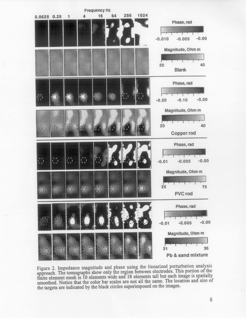
RESULTS AND DISCUSSION Data were collected on the four different targets described above using water as a medium of known and uniform resistivity (32 ohm-m). The results are displayed in Figures 2 (using the ERT algorithm for magnitude inversion and the PA algorithm for imaginary part inversion) and 3 (using the EIT algorithm).

3

The FE results are not shown because this approach did not yield reliable phase tomographs. Possible reasons for the poor performance are that the resistivity images are too noisy to accurately recover the relatively small changes in magnitude caused by the FE, and that the constant phase invalid for the targets used.

angle assumption inherent in the FE approach may be

We first examine the resistivity inversions performed by the ERT-PA algorithm (the magnitude plots in Figure 2). For the uniform resistivity case (water blank) the ERT images are approximately uniform at about 32 ohm-m at all frequencies except 1024 Hz. The ERT-PA approach is also able to reconstruct the position of the high contrast resistive model (PVC rod target), although it yields a low estimate (only 55 ohm-m reconstructed while the resistivity of PVC is above the MegaOhm-m range) for its magnitude. We should expect a poor reconstruction for a high contrast target since the code is stabilized with a spatially smooth, Occam’s type inversion. The smoothing has the effect of smearing the anomaly and reducing its contrast. For the highly conducting copper rod target, the ERT algorithm performs poorly, having trouble even locating the target position. If this problem were just one of high contrast, then the result should improve for the intermediate resistivity contrast case provided by the sand-lead target. However, the sand-lead target is also poorly resolved when phase information is ignored These observations suggest that impedance magnitude is reconstructed poorly when the target has a significant IP response and the IP data is ignored by the inversion algorithm.

Let us now compare the magnitude inversions which ignore IP data (ERT) with the magnitude inversions in Figure 3, where the reactive effects are included (EIT). These comparisons will help define what, if anything, has been gained by rigorously accounting for the reactance while calculating the magnitude tomographs. Both ERT and EIT yield nearly uniform 30 ohm-m images of the water blank target, for all frequencies. Similarly, the PVC target’s location, size, and contrast relative are rendered equally well by the EIT and ERT algorithms.

The EIT and ERT magnitude inversions of the copper rod target are disappointing, both methods showing relatively poor spatial resolution. The reason(s) for the poor performance are not fully understood although a conductive target in a relatively conductive medium is clearly more difficult to detect than a resistive target. Figures 2 and 3 indicate that spatial resolution and resistivity contrast of the copper rod improves with increasing frequency. We also observed that the measured transfer resistances for the raw copper rod data decreased with increasing frequency. Data from the other targets did not show this trend, thereby suggesting that the frequency dependent magnitudes are caused by decreases in contact impedance at the metal-electrolyte interface as the frequency increases. These results suggest that the spatial resolution of metallic objects in magnitude images can be improved by going to higher frequencies.

Surprising results are observed in the magnitude tomographs for the intermediate resistivity sand-lead target; this target creates conditions which are most similar to those encountered during field surveys. EIT magnitude inversions produced a well defined, weakly resistive anomaly of 35 ohm-m at 0.06265 Hz which decreased to.about 32 ohm- m at 16 Hz. Although it is positioned too close to the image center, there is no doubt that approximate target shape, size and location are evident; the same cannot be said for the tomographs recovered when the reactive effects were i reconstructed by the ERT algorithm). The complex alge fi

nored (Figure 2 magnitude ra algorithm (EIT) appears

superior to the algorithm using only real algebra (ERT) based strictly on comparisons of magnitude inversions. The sand-lead model results suggest that, when the reconstruction algorithms make proper use of the IP data, better magnitude reconstructions may be achieved.

4

Now let us consider any other possible benefits which may arise from inverting phase with an EIT algorithm, Both the water blank and the PVC targets should have no reactive component at these frequencies, given that there is no known mechanism for generating an IP signal. Except for the tomographs corresponding to higher frequencies, which are undoubtedly corrupted by data errors, we find that the phase images for both targets are less than about 10 milliradians. Although they are plotted to different scales, we can see that below 256 Hz the reconstructed phases are less than about 5 milliradians but are double that at 256 and 1024 Hz. This is consistent with figure 3 which clearly shows a much higher measured phase error at these two frequencies. The reconstructed phase values are therefore likely caused by these measurement errors propagating though the inversion algorithm. Images of the water blank serve to illustrate the effects of measurement error in the phase reconstructions of other targets. The error bounds inferred from these results are: 5 milliradians below 256 Hz and 10 milliradians at 256 and 1024 Hz.

We now consider the phase reconstruction for the copper rod target. Although we do not know what phase amplitude should be reconstructed for this target, the copper-electrolyte interface should produce a significant IP response. At all but the highest frequencies, the copper rod target is accurately located and is reconstructed as a capacitive reactance. A key observation is that the phase tomographs yield a more faithful representation of the target shape, location, and size than do the magnitude tomographs. These results reinforce the suggestion that inversion of impedance magnitude and phase (EIT) provide better resolution than inversion of resistance (ERT).

An equally important conclusion comes from the phase images of the sand-lead target. In this case, the phase response is about one twentieth that of the copper rod target, and it is above the noise level at frequencies below 256 Hz. Even more important is that the target was not clearly imaged by the ERT algorithm, but both the magnitude and phase reconstructions of EIT show the anomaly. These results indicate that measuring and inverting both the resistive and reactive portions of the earth response can help delineate targets better than what is possible with the resistive portion only. We suspect that this improvement results from additional target information contained in the IP data which serves as an additional constraint during minimization of the objective function (see equation 2).

The results from these tests consider only a limited range of experimental conditions and need verification under a wider range of conditions. Nevertheless, we suggest that the use of an EIT algorithm may be desirable because of the observed improvement in spatial resolution, even if the IP response is of no direct interest.

ACKNOWLEDGMENTS: This work was performed under the Earth and Environmental Sciences Directorate at LLNL. It was funded by the Characterization, Monitoring and Sensors Technology Program, Office of Technology Development, U.S. Department of Energy (DOE).

Work performed under the auspices of the U.S. Department of Energy by Lawrence Livermore National Laboratory under Contract W-7405-ENG-48.

REFERENCES Barber, D. C. ‘and A. D. Seagar, Fast reconstruction of resistance images, Clinical Physics and Physiological Measurement, 8; Suppl. A, 47-55,1987.

Daily, W. and E. Owen, Cross-borehole resistivity tomography, Geophysics, 56, 1228- 1235,199l.

Dines, K. A. and R. J. Lytle, 198 1, Analysis of electrical conductivity imaging, Geophysics, 46, 1025- 1036.

deGroot-Hedlin, C., and Constable, S., 1990, Occam’s inversion to enerate smooth, two- dimensional models from magnetotelluric data: Geophysics, 5.5, 16 3- 1624. H

Henderson, R. P. and J. G. Webster, An impedance camera for spatially specific measurements of thorax, IEEE Trans. Biomed, Eng, BME-25, 250-254, 1978.

Isaacson, D., 1986, Distinguishability of conductivities by electric current computed tomography, IEEE Trans. on Medical Imaging, vol. MI-J, no. 2,91-95, June.

LaBrecque, D. J., Miletto, M., Daily, W., Ramirez, A., and Owen, E., 1996, The effects of noise on Occam’s inversion of resistivity tomography data: Geophysics, 61,538-548.

Lytle, R. J. and K. A. Dines, 1978, An impedance camera: A system for determining the spatial variation of electrical conductivity, Lawrence Livermore Laboratory, Livermore, California, UCRL-524 13.

Oldenburg, D. W. and Y. Li, 1994, Inversion of induced polarization data, Geophysics, vol. 59, no. 9, pp 1327-1341.

Pelton, W. H., L. Rijo and C. M. Swift, Jr., 1978, Inversion of Two-dimensional resistivity and induced-polarization data, Geophysics, 43, no. 4,788-803, June.

Sasaki, Y., 1992, Resolution of resistivity tomography inferred from numerical simulation, Geophysical Prospecting, 40, 453-463.

Shi, W., W. Rodi, and F. D. Morgan, 1998, 3D induced polarization Inversion using complex electrical resistivities, In: Proc. of Symposium on the Application of Geophysics to Engineering and Environmental Problems, Chicago, Mar. 22- 26,1998, p. 785 - 794.

Siegel, H. O., 1959, Mathematical formulation and type curves for induced polarization, Geophysics, 24, 547-565.

Tripp, A. C., G. W. Hohmann and C. M. Swift, Two dimensional resistivity inversion, Geophysics, 49, 1708-l 7 17, 1984.

Weller, A., M. Seichter, and A. Kampke, 1996, Induced polarization modelling using complex electrical conductivities, Geophysical Journal International, 127,. 387-398.

Wexler, A., B. Fry and M. R. Neuman, 1985, Impedance-computed tomography algorithm and system, Applied Optics, 24, no. 23,3985-3992, December.

Yorkey, T. J., J. G. Webster and W. J. Tompkins, 1987, Comparing reconstruction algorithms for electrical impedance tomography, IEEE Trans Biomedical Engineering, BME-34, no. 11,843-852, November.

Yuval, and D. W. Oldenberg, 1997, Computation of Cole-Cole parameters using IP data, Geophysics, 62, no. 2,436-448.

6

stainless steel electrodes 2 mm dia. 2 mm thick

Top View I

O-

PVLand copper rod

0 0 0 0 0 0 0 0 0 o-

4 36 cm

b

I

6 z

Figure 1. Experimental arrangement of the scale model used. Two rows of 10 stainless steel electrodes model a cross-borehole scheme. The setup exploited symmetry and allowed current flow only in a half space. Position and size of the target are shown to scale. The water tank walls are more than 10 dipole lengths from the retion of interest.

7

Magnitude, Ohm m

Blank

II Phase, rad ,

II -0.20 -0.10 -0.00

Magnitude, Ohm m

Copper rod

Phase, rad

-0.01 -0.005 -0.00

Magnitude, Ohm m

PVC rod 75

Phase, rad

-0.01 -0.005 -0.00

Magnitude, Ohm m

Pb &sand mixture

Figure 2. Impedance magnitude and phase using the linearized pevbatioq analysis approach. The tomographs show only the region between electrodes. ‘I@ portlou of the finite element mesh is 10 elements wide and 18 elements tall but each Image is spatially smoothed. Notice that the color bar scales are not all the same. The location and uze of the targets are indicated by the black circles superimposed on the images.

8

.-_1--..-1 ‘.-

0.0626 0.26 1 4 16 64 266 1024

Phase, rad

-0.010 -0.005 -0.00

Magnitude, Ohm m

20 40 Blank

Phase, rad

-0.20 -0.10 -0.00

Magnitude, Ohm m

20 40

Copper rod

PVC rod

Magnitude, Ohm m

Pb &sand mixture

Figure 3 Impedance magnitude and phase using the EIT approach. The tomographs show only the region between electrodes. Other mesh details are the same as indicated for Figure 2.

9