NBER WORKING PAPER SERIES

LABOR RATIONING

Emily BrezaSupreet Kaur

Yogita Shamdasani

Working Paper 28643http://www.nber.org/papers/w28643

NATIONAL BUREAU OF ECONOMIC RESEARCH1050 Massachusetts Avenue

Cambridge, MA 02138April 2021

We thank Abhijit Banerjee, David Card, Andrew Foster, Jessica Goldberg, Pat Kline, Jeremy Magruder, Ben Olken, Duncan Thomas, and many seminar participants for helpful comments and conversations. We thank Arnesh Chowdhury, Piyush Tank, Silvia Wang, Mohar Dey, Anshuman Bhargava, Vibhuti Bhatt, Asis Thakur, and Anustubh Agnihotri for excellent research assistance. We gratefully acknowledge financial support from the National Science Foundation. The views expressed herein are those of the authors and do not necessarily reflect the views of the National Bureau of Economic Research.

NBER working papers are circulated for discussion and comment purposes. They have not been peer-reviewed or been subject to the review by the NBER Board of Directors that accompanies official NBER publications.

© 2021 by Emily Breza, Supreet Kaur, and Yogita Shamdasani. All rights reserved. Short sections of text, not to exceed two paragraphs, may be quoted without explicit permission provided that full credit, including © notice, is given to the source.

Labor RationingEmily Breza, Supreet Kaur, and Yogita ShamdasaniNBER Working Paper No. 28643April 2021JEL No. E24,J2,J6,O10,O17

ABSTRACT

This paper measures excess labor supply in equilibrium. We examine hiring shocks—which employ 24% of the labor force in external month-long jobs—in Indian local labor markets. In peak months, wages increase instantaneously and local aggregate employment declines. In lean months, consistent with severe labor rationing, wages and aggregate employment are unchanged, with positive employment spillovers on remaining workers—indicating that over a quarter of labor supply is rationed. At least 24% of lean self-employment among casual workers occurs because they cannot find jobs. Consequently, traditional survey approaches mismeasure labor market slack. Rationing has broad implications for labor market analysis.

Emily BrezaHarvard UniversityLittauer Center, M281805 Cambridge StreetCambridge, MA 02138and NBERebreza@fas.harvard.edu

Supreet KaurDepartment of EconomicsUniversity of California, BerkeleyEvans HallBerkeley, CA 94720and NBERsupreet@berkeley.edu

Yogita ShamdasaniNational University of Singaporeyogita@nus.edu.sg

LABOR RATIONING 1

1. Introduction

[D]istinguishing elements of voluntariness from elements of involuntariness inthe unemployment problem is a hopeless endeavour. (Fellner, 1976)

In developing countries, wage employment rates among rural workers often hover around50%. For example, Indian landless prime age males—whose primary source of earnings iswage labor—work 45.7% of the time (NSS 2009). In Bangladesh, wage employment rates forlandless males are about 55% in lean months (Akram et al., 2018). In Sub Saharan Africa,these rates are typically even lower (Beegle and Christiaensen, 2019).

The interpretation of this empirical regularity is unclear, and has long been a source of de-bate. Research going back to Lewis (1954) argues that low employment reflects extremelyhigh involuntary unemployment, indicating large distortions. However, other work has shownthat these labor markets adjust rapidly to changing market conditions (e.g., Rosenzweig,1988). Thus, low wage work might instead be the outcome of reasonably well-functioninglabor markets, where workers are simply choosing other activities such as self-employment.These two possibilities have drastically different implications for the labor market equilib-rium. Moreover, while the development labor literature has documented frictions—givingrise to separation failures, labor misallocation, and downward wage rigidity (e.g., LaFave andThomas, 2016; Bryan et al., 2014; Kaur, 2019)—knowing that these exist does not tell usabout the extent of aggregate distortions in equilibrium. In other words, existing work can-not explain how one should interpret observed employment patterns. Specifically, whetherthere is a large amount of labor rationing in this setting still remains unknown.

This paper empirically assesses the extent to which labor supply exceeds labor demand inequilibrium. For concreteness, we define a worker as rationed if: a) she would prefer wageemployment at the current market wage over what she is doing (i.e. the worker is not on herlabor supply curve), and b) the worker is employable at that wage (i.e. from the employer’sperspective, her marginal product is weakly above the current wage). A rationed worker maybe involuntarily unemployed, or engaged in another activity such as self-employment.

Determining the amount of rationing presents challenges under current approaches. To mea-sure involuntary unemployment, economists use survey self-reports—whether an individualwas looking for a job but could not find one. However, the validity of this approach hasbeen questioned, and remains unknown (e.g. Bound et al., 2001; Taylor, 2008). These chal-lenges are exacerbated in developing countries, where self-employment is prevalent and canabsorb workers who cannot find jobs. While previous work discusses the presence of such“disguised” or “hidden” unemployment, we currently have no estimates of whether a sizablefraction of self-employment is due to rationing in the wage labor market.

LABOR RATIONING 2

We tackle these fundamental measurement problems by developing a simple revealed pref-erence approach to test for excess labor supply (i.e. labor rationing). We induce transitoryhiring shocks in Indian local labor markets—giving jobs to on average 24% of the labor forceof casual male workers in external jobsites for 2-4 weeks. This shock substantively reduceshow many workers remain in the local economy, without changing local labor demand.1

We then use the local labor market response to learn about the equilibrium that existedin the absence of our shock. We take seriously the idea that seasonality in labor demandmay be consequential for labor market functioning (Leibenstein, 1957), with relevance forunderstanding seasonal fluctuations in employment levels (Bryan et al., 2014; Fink et al.,2018). Consequently, we undertake this exercise across the year—enabling us to test forexcess supply separately across lean and peak months.

This approach uncovers labor market functioning without direct intervention on the partici-pants of interest. While we exogenously generate shocks, the outcomes are driven completelyby the response of existing employers and workers who never interface with the external job-sites. We use the phrase “local labor market” to denote all jobs, wages, and employmentexcluding the external worksite jobs we create. If the level of rationing is higher than the sizeof our shock—e.g., if we remove 25% of the labor force and more than 25% of worker-daysare rationed—then we would expect the following local labor market impacts: i) no changein wage levels; ii) no effect on aggregate employment; and iii) positive employment spilloverson individual workers whose employment goes up due to less competition for jobs. Thisconstitutes a revealed preference test of rationing driven by a failure of wage adjustment.Specifically, workers reveal they prefer jobs at the market wage over their previous activity(e.g. unemployment or self-employment), and employers reveal the worker is qualified fora job at the market wage. If these predictions hold, the size of our hiring shock is a lowerbound on the level of excess labor supply in the economy.

This design diagnoses rationing without assumptions about the equilibrium in the absenceof rationing—for example, whether it is fully competitive or subject to monopsony or someother friction. We view this as a strength of our approach, and do not make direct claimsregarding potential other frictions.

The setting for our test is rural labor markets in Odisha, India, which exhibit many features ofdeveloping country village economies—including low wage employment and high seasonality.We conduct the experiment using a matched-pair, stratified design in 60 labor markets (i.e.villages) across varying times of the year. We invite workers to sign up for employment at1We discuss the possibility of multiplier effects from demand below.

LABOR RATIONING 3

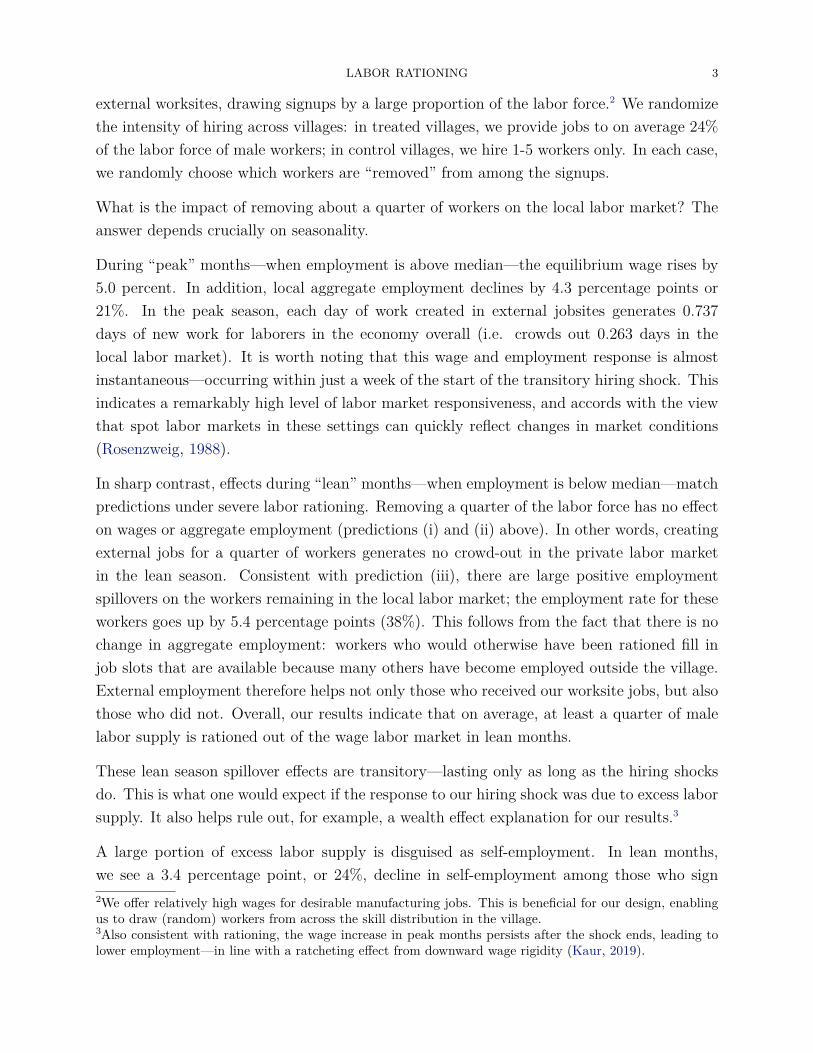
external worksites, drawing signups by a large proportion of the labor force.2 We randomizethe intensity of hiring across villages: in treated villages, we provide jobs to on average 24%of the labor force of male workers; in control villages, we hire 1-5 workers only. In each case,we randomly choose which workers are “removed” from among the signups.

What is the impact of removing about a quarter of workers on the local labor market? Theanswer depends crucially on seasonality.

During “peak” months—when employment is above median—the equilibrium wage rises by5.0 percent. In addition, local aggregate employment declines by 4.3 percentage points or21%. In the peak season, each day of work created in external jobsites generates 0.737days of new work for laborers in the economy overall (i.e. crowds out 0.263 days in thelocal labor market). It is worth noting that this wage and employment response is almostinstantaneous—occurring within just a week of the start of the transitory hiring shock. Thisindicates a remarkably high level of labor market responsiveness, and accords with the viewthat spot labor markets in these settings can quickly reflect changes in market conditions(Rosenzweig, 1988).

In sharp contrast, effects during “lean” months—when employment is below median—matchpredictions under severe labor rationing. Removing a quarter of the labor force has no effecton wages or aggregate employment (predictions (i) and (ii) above). In other words, creatingexternal jobs for a quarter of workers generates no crowd-out in the private labor marketin the lean season. Consistent with prediction (iii), there are large positive employmentspillovers on the workers remaining in the local labor market; the employment rate for theseworkers goes up by 5.4 percentage points (38%). This follows from the fact that there is nochange in aggregate employment: workers who would otherwise have been rationed fill injob slots that are available because many others have become employed outside the village.External employment therefore helps not only those who received our worksite jobs, but alsothose who did not. Overall, our results indicate that on average, at least a quarter of malelabor supply is rationed out of the wage labor market in lean months.

These lean season spillover effects are transitory—lasting only as long as the hiring shocksdo. This is what one would expect if the response to our hiring shock was due to excess laborsupply. It also helps rule out, for example, a wealth effect explanation for our results.3

A large portion of excess labor supply is disguised as self-employment. In lean months,we see a 3.4 percentage point, or 24%, decline in self-employment among those who sign2We offer relatively high wages for desirable manufacturing jobs. This is beneficial for our design, enablingus to draw (random) workers from across the skill distribution in the village.3Also consistent with rationing, the wage increase in peak months persists after the shock ends, leading tolower employment—in line with a ratcheting effect from downward wage rigidity (Kaur, 2019).

LABOR RATIONING 4

up for worksite jobs. By revealed preference, these business owners prefer wage labor atthe prevailing wage to working in their businesses. This implies that in our sample, in thelean season, at least 24% of self-employment stems from workers being rationed out of wagelabor. Among farm households, these effects are entirely concentrated among those withbelow median per-capita landholdings—the group we would expect to be most affected bya ration in the labor market. Workers in these households reduce self-employment by 7.2percentage points (50%)—indicating that on small farms, half of self-employment in leanmonths is driven by rationing. Like the employment spillovers, these effects are also tran-sitory. Once the shock ends, self-employment levels between treatment and control villagesare indistinguishable—ruling out the concern that business owners simply intertemporallysubstitute by increasing self-employment in the future.

Finally, we examine traditional survey-based unemployment measures. Despite the sizableimpacts on wage employment, overall work status does not move in lean months—preciselydue to disguised unemployment. In addition, if we mimic the approach for measuring involun-tary unemployment used in government surveys (including India’s National Sample Survey),we would conclude that our shocks had no impact on unemployment in lean months. Weevaluate an alternate survey measure, and find its movement matches the revealed preferencemagnitudes. However, our findings suggest that, in our setting, traditional survey questionswill mismeasure the extent to which individuals are unable to find wage work.

We argue that other potential mechanisms through which the shocks could affect wages oremployment—such as a local demand expansion from increased wealth, or a change in workercomposition—cannot explain our pattern of results. We also offer direct tests for such poten-tial confounds, and rule out perfectly elastic labor supply. In addition, we evaluate potentialmicro-foundations for excess labor supply—such as efficiency wages, dynamic contracting,implicit insurance, and worker collective action—in light of our findings.

Overall, the patterns we document are consistent with the hypothesis of “under-utilizedlabor” proposed by Leibenstein (1957). If the labor market, and particularly the wage, doesnot adjust fully to seasonal reductions in labor demand, this can generate rationing in leanperiods. While our estimates are of course specific to our particular context, the patternof differences in labor market functioning across peak and lean times is likely more general.Similar dynamics plausibly prevail in many rural, developing country settings.

Our results have implications for labor market policies, such as workfare—implying thatcrowd-out will depend crucially on the level of slack. In a suggestive exercise, we examinethe phased-in roll-out of India’s workfare program, NREGA (Imbert and Papp, 2015). Whenslack is higher (i.e. baseline district-month employment is lower), NREGA has no detectable

LABOR RATIONING 5

impact on wages or private employment. However, when the labor market is tighter, wagesrise and agricultural employment falls by almost 20%, indicating substantial crowd out.These patterns match our experimental findings. Note that we don’t rule out the possibilityof lean season wage increases more generally: if a shock is larger than the number of rationedworkers or changes reservation wages, wages could rise even in lean times.

This paper provides novel evidence on the functioning of labor markets in poor countries.It offers the first direct evidence that labor supply substantively exceeds labor demand inequilibrium. The earliest work in development, such as the surplus labor hypothesis, waspremised on the view that rural economies have large slack (Lewis, 1954). The empiricalrelevance of this view has been unclear, especially in modern times. We document consider-able slack, indicating that at least a quarter of labor supply is rationed during lean months.These findings suggest that moving rural workers to other sectors—where their labor maybe more readily absorbed—could increase aggregate output not simply due to TFP differ-ences between sectors (Gollin et al., 2014; McMillan and Rodrik, 2011), but also by enablingrationed workers to be employed.4

We also provide the first estimates of how much of self-employment is actually “disguisedunemployment” (i.e., “forced entrepreneurship”). A striking share of self-employment in oursample—23% on average and 75% among smallholder farms—would not occur if businessowners could find work at the prevailing wage in lean months. This helps further our un-derstanding of a prominent empirical fact: why self-employment is so high in poor countries(e.g. Banerjee and Duflo, 2007; De Mel et al., 2010).5

Relatedly, we advance the literature on labor market frictions in poor countries. A large bodyof work has examined separation failures (Singh et al., 1986; Benjamin, 1992; Fafchamps,1993; Udry, 1996; LaFave and Thomas, 2016; Dillon et al., 2019; Jones et al., 2020; LaFaveet al., 2020). These studies do not take a stance on the exact distortion that generatesthe failure—rationing or some other friction.6 They also do not quantify how many firmsare affected.7 Our findings complement this work by tracing the first direct link from laborrationing to separation failures, and showing that rationing increases self-employment on4Our design relates to tests of surplus labor (Schultz, 1964; Sen, 1967; Donaldson and Keniston, 2016). Whileother work has documented low employment levels during lean months, our study is the first to link thisto rationing, rather than simply market clearing with low employment demand. Note that the presence ofrationing complicates the interpretation of analyses that rely on wage differences across sectors to infer TFPdifferences.5Adhvaryu et al. (2019) document that coffee farmers increase non-agricultural self-employment when farmingbecomes less profitable, though this does not require any market frictions such as rationing.6See Behrman (1999) for a review. Pitt and Rosenzweig (1986) test a different microfoundation: productivityof own vs. hired labor. Foster and Rosenzweig (2017) examine the implications of transaction costs in hiring.7E.g., the comparative static of whether household size affects farm labor use tests for a failure of separability,but does not shed light on whether the associated labor supply distortion affects 1% or 50% of workers.

LABOR RATIONING 6

the majority of smallholder farms. More broadly, while previous studies have documentedfrictions—including separation failures, wage rigidity (Kaur, 2019), and worker collusion(Breza et al., 2019)—they are not designed to tell us whether the magnitudes are ultimatelyconsequential for labor market functioning. Our design is built solely to address this question,offering the first evidence that the labor market is, at times, severely distorted.

At the same time, our finding of instantaneous adjustment in peak months supports the viewthat spot labor markets can be quite flexible—consistent with studies showing robust labormarket adjustment to shocks (e.g. Rosenzweig, 1988; Jayachandran, 2006; Imbert and Papp,2015; Donaldson and Keniston, 2016; Akram et al., 2018; Breza and Kinnan, 2018; Muralid-haran et al., 2020; Egger et al., 2019). Our results therefore reconcile these studies withthose above, providing a more complete characterization of labor market functioning.

Our methodological approach also contributes to the literature on measuring unemploymentand labor market slack. To date, economists have measured involuntary unemployment usingsurvey self-reports, whose reliability is difficult to ascertain (e.g. Bound et al., 2001; Taylor,2008; Card, 2011; Faberman and Rajan, 2020). We stack survey responses against our re-vealed preference findings, documenting the unreliability of such measures. We highlight thiscan be particularly problematic when rationed workers are likely to switch to other activities,such as self-employment or gig economy jobs. In addition, we build on previous work, whichhas documented heterogeneity in employment crowd-out from shocks (e.g. Crepon et al.,2013; Gautier et al., 2018). Through precise information on the shock size and by samplingoutcomes for the entire labor force, we provide the first revealed preference estimates for theextent of rationing in the economy in any setting.

Finally, our research design provides a cleaner test of excess labor supply relative to otherpotential approaches, such as offering jobs to the unemployed. In practice, the implementa-tion of this approach has not provided a straightforward test. For example, in Breza et al.(2019), employers are compensated to offer jobs, search costs are eliminated, and the matchto workers is randomly assigned. Consequently, it is unclear whether either of the two cri-teria for rationing is satisfied, making it impossible to quantify rationing.8 In addition, ourdesign enables a fuller picture of excess supply and its implications, including the essentialrole of seasonality, effects on self-employment, and private-sector crowd-out—which requiresexamining the interaction of labor supply and demand in equilibrium.

Our findings have broad implications for labor market analysis and policy. First, the absenceof lean-season market clearing implies that the wage does not always play an allocative role.Thus, analyses that use wages to infer the marginal product of labor, for example, may8Specifically, workers who accepted jobs may not be considered qualified by employers in the absence of thewage subsidy, and may not have preferred the job under natural search and matching conditions.

LABOR RATIONING 7

be misleading. Second, our findings are relevant for predicting the effects of labor marketprograms, such as workfare (Imbert and Papp, 2015; Beegle et al., 2017; Bertrand et al.,2017; Zimmermann, 2020; Muralidharan et al., 2020). Specifically, heterogeneity in slackmay help explain why some programs have substantive labor market impacts while othershave virtually none.9 Finally, our finding of large quantities of “forced entrepreneurship” canhelp explain why policies that direct resources to small firms have only had limited successfor the average firm (e.g., McKenzie and Woodruff, 2014; Banerjee et al., 2015).

The remainder of the paper is organized as follows. Section 2 describes the context. Section3 outlines our hypotheses and predictions. Section 4 details the implementation and Section5 describes the data. We present the results in Sections 6 and 7. Section 8 discussesmicrofoundations and potential threats to validity. Section 9 offers suggestive extensions,such as heterogeneity in the impact of India’s workfare program. Section 10 concludes.

2. Context

Our field experiment takes place in villages across five districts in rural Odisha, India. Mar-kets for casual daily labor are extremely active in our setting specifically, and constitute anemployment channel for hundreds of millions of workers in India more generally (NationalSample Survey, 2010). The village constitutes a prominent boundary for the casual labormarket — daily-wage workers typically find jobs in both agriculture and non-agriculturewithin or close to their own village. This local nature of hiring is a necessary condition forour experimental hiring shocks to have a meaningful impact on the aggregate labor supplyfacing firms and on the labor market equilibrium.

The casual labor markets in the study areas are characterized by the same decentralizationand informality as much of India (e.g. Rosenzweig, 1988; Dreze et al., 1986). Contracting isusually bilaterally arranged between employers and workers a few days before the start ofwork. Moreover, the typical job lasts 1-3 days. This short duration of employment contractscreates the potential for transitory labor supply shocks to quickly impact wages. Labordemand is typically infrequent and variable. As in much of India, agricultural labor demandis seasonal, and both agricultural and non-agricultural jobs tend to be task-based (Fosterand Rosenzweig, 2017). For example, an employer might hire a different group of 5 workersto weed his paddy fields once or twice in a season, or a skilled roof-thatcher may hire adifferent assistant each time he is hired to rethatch a roof in the village.

Hiring is also employer-directed. 98% of agricultural employers report typically approachingworkers, by physically going to the neighborhoods where workers live, to fill hiring needs.9E.g., Beegle et al. (2017) find no workfare crowd-out in Malawi, and hypothesize this may be due to slack.

LABOR RATIONING 8

Given the intermittent nature of an individual employer’s labor demand, a typical agricul-tural employer in our sample only hires workers for six days per month. Thus, workerswork for many different employers, and each employer works with many different workers.Because rural villages tend to be relatively small and engage in labor relationships everyyear, employers and workers within a village tend to know one another. For example, whenasked to rate the quality of workers in the village, surveyed employers reported not knowinga randomly-chosen worker only 27.9% of the time. In addition, non-agricultural employersalso recruit by driving into the village and picking up workers who are available at the timein trucks.10

In our context, labor markets are not fully integrated spatially. For example, employersmust pay higher wages to workers who are hired from outside their village, in part dueto transportation costs and commuting time. In our data, this amounts to a 12% wagepremium. In addition, workers believe their village-level collective labor supply decisionsaffect village wages (Breza et al., 2019). This would not be possible under fully integratedmarkets.

Consistent with the seasonal, project-based nature of labor demand, employment rates in thecasual labor market are highly variable, higher in “peak” months and lower in “lean” months.Wage employment rates fall by more than 40% from peak to lean months. The villages inour study match a general feature of village economies: large periods of low employment(Muralidharan et al., 2020; Dreze et al., 1986).

Self-employment is extremely common in our setting. Among the workers who sign up forthe external jobs that form the basis of our hiring shock, 67% own land, while 88% have somekind of household business. Common household businesses reported in our context includegrocery store owners, street vendors, vegetable sellers and firewood collectors. However,businesses tend to have low levels of capital and small land-holdings, especially for thosecultivators who are also engaged in casual labor.

We also note that while India has a well-known workfare program, the National Rural Em-ployment Guarantee Act (NREGA), it is not very well implemented in Odisha. In principle,NREGA offers 100 days of employment in public works annually, but the average employmentrate in public works in our sample is 0.5%.11

10Workers also obtain non-agricultural work by commuting to district towns, though this is less common inour specific context.11In their analysis of NREGA, Imbert and Papp (2015) discuss the vast heterogeneity in program implemen-tation across India; Odisha is notably absent from their list of high-performing states. Moreover, in the NSSdata used by Imbert and Papp (2015), respondents in our 5 study districts (2 of which were early programdistricts), reported zero days of public works employment. Our more recent survey data indicate that thestate’s implementation issues have persisted.

LABOR RATIONING 9

Finally, in Table 1, we use data from the 2011 Indian Census to show how our study villagescompare to the average village in the five districts in Odisha where the experiment was run.The study villages are slightly smaller than average, with 148 households per village in thesample, compared to 176 households overall (p-val=0.299). However, our sample villages arecomparable on most dimensions. For example, 67.8% of residents are literate in our samplecompared to 66.1% overall (p-val=0.428), and 74.5% of males participate in the labor marketin our sample compared to 76.9% across all villages (p-val=0.306).

3. Hypotheses

3.1. Definition of Labor Rationing. Suppose the prevailing wage for one day of workin the casual daily market is w.12 We define a worker as rationed on a given day when thefollowing two conditions hold: (i) The worker wants to supply labor at wage w, but is unableto find employment; (ii) The worker is qualified for jobs occupied by other villagers.

The first condition states that the worker is not on her labor supply curve. The secondcondition states that a worker who wants a job but is unqualified for it (in the sense thatan employer would never find it profitable to hire her at wage w) is not considered rationed.Note that this takes no stance on the micro-foundation for rationing.

3.2. Predicted Impacts of a Hiring Shock. The core of our design is an experimentalhiring shock, through which a (random) subset of workers in the local labor market is hiredin external jobs outside the village. To diagnose rationing, we examine the effects of thisshock on local wages and employment—i.e., wages and employment in the local labor market,excluding the external worksite jobs we create.

We model the experimental hiring shock as a supply shock to the local labor market. Throughour intervention, some workers are “removed” and placed in external jobsites. This consti-tutes a reduction in the residual labor supply available to employers in the village; in otherwords, the (residual) village labor supply curve shifts to the left. However, this modelingchoice is not consequential for our test. As we discuss below, we could model this as ademand shock instead and would arrive at the exact same predictions for local wages andemployment under rationing.13

To lay out our predictions, we employ the simplest framework to interpret our results: astylized demand and supply framework. Panel A of Figure 1 shows the effects of a negativelabor supply shock under market clearing. Let E denote the level of local employment (in12Our results hold if we use hourly wages as the basis for our definition instead.13Under the typical definition of a demand shock, we would have posted the jobs, and then, as price takers,hired workers at whatever equilibrium wage prevailed after posting. Instead, we purposely choose whichworkers to “remove” at a pre-determined (high) wage. This parallels, e.g., workfare programs, which are alsotypically modeled as supply shocks to the local private sector.

LABOR RATIONING 10

terms of worker-days) in the village and w denote the village wage in the absence of ourintervention. A supply shock (a shift from S to S ′) will:

P1) Increase local wages from w to w′;

P2) Decrease aggregate employment among workers who remain in the village (i.e. thosewho are not hired by us to work in jobsites), so that total employment after the shockE ′ is less than E.

Panel B of Figure 1 shows the effects of a negative labor supply shock when there is excesslabor supply. As before, E denotes the level of employment in the village and w denotes thevillage wage in the absence of our intervention. Rationing exists in this labor market, withsupply ES exceeding demand ED at wage w. Employment levels are therefore determinedby the labor demand curve. If the amount of labor rationing is weakly greater than the sizeof the supply shock, then we predict that the shock (a shift from S to S ′) will have:

L1) No effect on local wages (the wage remains w);

L2) No effect on aggregate employment levels (aggregate employment remains E);

L3) Positive employment spillovers on individual workers, whose employment goes up dueto reduced competition for job slots.

Note that these predictions are not sensitive to whether S ′ is a parallel shift of the supplycurve; they hold even if the supply elasticity changes (i.e. due to a non-parallel shift). Ifpredictions L1-L3 hold, the size of our hiring shock is a lower bound on the level of rationingin the economy.

Note that predictions L2 and L3 above are inherently related. Under rationing, workers whowould have otherwise been rationed fill in job slots that are now available because many otherlaborers competing for the same jobs have become employed outside the village. The resul-tant increase in the proportion of days employed among remaining workers is why aggregateemployment remains unchanged. Appendix Figure A.1 validates that predictions L1-L3 holdunder rationing if we model the hiring shock as a positive demand shock instead.14

This constitutes a revealed preference test for excess labor supply: If predictions L1-L3 hold,workers reveal that they prefer jobs at w over their previous activity (e.g. unemployment or14As Appendix Figure A.1 makes clear, we would expect: (i) no change in the wage, and (ii) aggregateemployment (including the external hiring shock jobs) would increase one-for-one with the size of the hiringshock—implying no change in aggregate local village employment (i.e. excluding the hiring shock). Thiscorresponds exactly to Predictions L1 and L2, respectively, and L3 follows mechanically from L2.

LABOR RATIONING 11

self-employment), and employers reveal that workers are qualified to be hired for the jobs atw.15

To enrich our understanding of labor market functioning, we undertake the above exerciseacross different months of the year. This is motivated by earlier work in the developmentlabor literature, which argued that seasonality in labor demand is consequential for shapinglabor market equilibrium at different times of the year (e.g. Leibenstein, 1957; Dreze andMukherjee, 1989). Consistent with this work, we hypothesize that the peak season effects ofhiring shocks will be closer to those in Panel A of Figure 1, whereas the lean season effectswill match those in Panel B.

3.3. Self-employment and Disguised Unemployment. If there is excess supply, ra-tioned individuals may appear as unemployed or may turn to less-productive self-employmentas a way to generate income—creating “disguised unemployment” or “forced entrepreneur-ship” (Singh et al., 1986). For this group, self-employment earnings are below w, but abovetheir reservation wage.

Consequently, under rationing, when job slots open up through the hiring shock, a fractionof both unemployed and/or self-employed workers will reveal that they prefer jobs at theprevailing wage w over what they were previously doing. Among business owners, the mag-nitude of this shift will provide a lower bound on the fraction of self-employed workers whoare disguised unemployed.16

3.4. Discussion of Predictions. Predictions L1-L3 diagnose rationing, with minimal otherassumptions about the labor market. For example, our test does not require assumptionsabout the equilibrium in the absence of rationing—whether it is fully competitive (ED = ES)or subject to monopsony or some other friction (ED > ES). For example, if there weremonopsony in the labor market but no rationing, then our hiring shock would necessarilylead to an increase in wages—contradicting prediction L1 (see Appendix Figure A.2).17

15To illustrate these predictions, consider the following thought exercise. Suppose 10 workers want work inthe village at wage w, but only 5 job slots are available. As a result, 5 workers are employed at w, whilethe other 5 workers are rationed: the employment rate is 50%. Now, suppose we remove 4 workers fromthe village labor market. This frees up job slots, and a larger portion of the remaining workers can nowwork in the village at wage w. Specifically, there are 6 workers left who want work and still 5 availableslots: the employment rate is now 83%. In contrast, if the 5 workers who are unemployed did not wantwork, they would not accept employment at wage w; this provides a test of condition (i) in the rationingdefinition above. In addition, the fact that workers who remain in the village are hired at wage w indicatesthat employers perceive them as qualified for work at w; this provides a test of condition (ii) above.16Since we do not take a stance on the rationing mechanism, we do not have an ex ante prediction on whetherunemployed or self-employed workers are more likely to be hired into empty job slots first. In addition, ifthere are fixed costs of stopping and then going back to one’s business, then this is another reason why theestimates from this exercise will be a lower bound on disguised unemployment.17If our hiring shock simply shifts the labor supply curve to the left, then the predictions under monopsonyare unambiguous—wages should rise and employment should fall. However, if the shock also changes the

LABOR RATIONING 12

In addition, we do not take a specific stance on the reason for rationing; our test is validfor a range of microfoundations. Overall, our test is chiefly powered to detect rationing thatis generated by some failure of wage adjustment to seasonal reductions in labor demand.Rationing from effort efficiency wages (Shapiro and Stiglitz, 1984), for example, would notgenerate the patterns we hypothesize. There, wages would respond to a reduction in laborsupply: because the hiring shock would lower the cost of unemployment, wages would needto increase to restore incentives. Section 8.1 discusses microfoundations in light of ourresults.

We also do not need to specify the rationing mechanism i.e. how jobs are allocated acrossworkers. There may be a distribution of ability levels among rationed workers, and thisdistribution could even change with the shock. However, if we observe predictions L1 andL3, it must be the case that there are workers in the village who prefer wage jobs andemployers are willing to hire them for those jobs at the prevailing wage w—satisfying thetwo criteria in the definition for rationing.

Note that a key feature of our research design is that we can precisely quantify what fractionof the labor force is “removed” through the hiring shock because our shocks are targeted —available only to some workers who are offered the external jobs (see below). This standsin contrast to other labor market shocks such as workfare programs, which are permanentand impact all eligible workers by offering an outside option. This potentially increasesreservation wages and shifts the labor supply curve even among workers who do not everparticipate directly, making it difficult to know what fraction of workers is affected. Conse-quently, it would be difficult to use a shock such as a workfare policy to quantify rationing.Our transitory targeted shocks greatly simplify analysis, enabling us to bound the level ofrationing without needing to impose assumptions about labor supply responses.

4. Experiment: Design and Implementation

We engineer transitory hiring shocks in study villages. We exploit an opportunity to recruitcasual male workers for full-time manufacturing jobs for 2-4 weeks.18 The work occurs inexternal jobsites within daily commuting distance from study villages.19 Such temporaryone-time contract jobs are a common source of non-agricultural employment for men in theregion. The external jobs are attractive — the daily wage is weakly higher than the prevailingmarket wage for casual labor, and there are positive compensating differentials (e.g., the work

labor supply elasticity facing the employer, then wages would still increase, but the employment effect isambiguous. One example is the canonical case of an increase in the minimum wage. See Chapter 2 ofManning (2013) for a detailed discussion.18In this cultural context, women are unwilling or unable to travel outside of the village for work.19We leverage two separate field projects (Breza et al., 2018; Kaur et al., 2019) that involve hiring workersfor low-skill manufacturing jobs. See Appendix C for a full description of these jobs.

LABOR RATIONING 13

occurs indoors and is not very physically demanding). This offers an advantage because itdraws interest from many workers in the village, enabling us to (randomly) draw from asizable swath of the labor force.

The external jobs are advertised in villages through flyers, village meetings, and door-to-doorvisits to male adults. Hired workers are then drawn randomly from the subset of the villagelabor force that signs up for the job. See Appendix C for more details about the recruitmentprotocols and external jobs.

We randomize recruitment intensity at the village (i.e. local labor market) level, so that intreatment villages we hire up to 60% of sign ups, and in control villages we hire 1-5 workersonly.20 We thus generate a large hiring shock in treatment villages, and a negligible shock incontrol villages. We use a matched-pair, stratified research design, so as to achieve balanceby local region and time.

We implement these shocks in different months of the year, which correspond to differentlevels of labor demand and employment. We limited our experiment to ten months of thecalendar year, omitting the two busiest months—August (peak planting) and December(harvesting)—so as to not affect labor supply during important work periods. Thus, ourexperiment does not run in the pure peak season, but rather in the lean and semi-peak (orshoulder) months.

We use employment rates in control villages as our proxy for underlying labor market slack.Months with above-median employment rates are classified as semi-peak periods, whilemonths with below-median employment rates are classified as lean periods of the year.

We run the experiment in 60 villages (labor markets) across 5 districts in Odisha, India,between the years 2014 to 2018. We used a matched-pair randomization design, so we have30 treatment and 30 control villages. 43% of the experimental rounds were conducted inlean months, and the remaining 57% in semi-peak months. We have survey data for 2,379workers in total.

Our experiment only has power to detect rationing if the labor market is not fully integratedacross villages—so that removing workers in one village constitutes a meaningful local sup-ply shock from employers’ perspective. Under full labor market integration, we would not20We set this limit of 60% in order to ensure there were enough workers left over in the village to comprisea substantive spillover sample (on whom we could observe treatment effects), and to avoid the possibilitythat the shock ended up being larger than the amount of rationing in lean seasons. In addition, we hiredno more than approximately 30 workers per village due to space constraints at the external worksites. Notethat workers were told in advance that the number of job slots would be determined based on contractorneeds, so that ex ante beliefs about hiring probability were the same across treatment and control villages.

LABOR RATIONING 14

expect to find wage adjustment from our hiring shock in either the lean or semi-peak season.Moreover, even in the presence of rationing, we would not detect employment spillovers.

The lack of full integration is a reasonable assumption in our context. Agricultural hiringoccurs primarily within the village, as described in Section 2 above. In addition, even fornon-agricultural jobs, it is common for contractors to recruit by coming to a village andloading (a predetermined number of) workers onto a truck—providing scope for employmentspillovers even for jobs conducted outside the village.

5. Empirical Strategy and Data

5.1. Analysis Samples. Figure 2 summarizes the analysis samples across control villages(Panel A) and treatment villages (Panel B). The dark grey areas denote workers who signup for the jobs and are “removed” to work in the external jobsites. The light grey shadedareas denote workers who sign up but are not offered jobs — these workers remain in thevillage and constitute our intent-to-treat sample. We refer to these workers hereafter as thespillover sample. Note that the spillover sample is larger in control villages (Panel A), sinceonly 1-5 workers are offered jobs in control villages.

For the analysis, we examine effects on two sets of samples. The first is the spillover sam-ple, which is directly comparable to the workers who were removed from the village, andtherefore would be most likely to benefit from employment spillovers. The second is allpotential workers in the village—regardless of whether they signed up for our jobs—in orderto accurately assess effects on aggregate employment levels.

5.2. Estimation Strategy. To test how the experimental hiring shock impacts employmentand wages, we compare outcomes in treatment and control villages, separately for semi-peakand lean months. Our base specification is:

(1) yitvr = α + βHiringShockv + γHiringShockv ∗ SemiPeakr + ρr + X0ivr + εitvr

where yitvr is an outcome for worker i on day t in village v and experimental round r.HiringShockv is an indicator for treatment villages, and SemiPeakr is an indicator forexperimental rounds conducted in semi-peak months. We include the worker’s baseline meanemployment rate and mean daily wage levels X0

ivr in order to increase precision (and we alsoreport estimates without baseline controls). Regressions always include round (strata) fixedeffects (ρr), and cluster standard errors by village.

To construct the SemiPeakr indicator, we calculate the mean month-wise employment ratein control villages for each month in our sample, averaging across all rounds that started ina given month (See Appendix Figure A.3). We then take the median of this variable across

LABOR RATIONING 15

rounds in the sample. Months with above-median values are classified as semi-peak periodsof the year. In addition, in the analysis, we show robustness to replacing the SemiPeakr

binary variable with the continuous month-wise employment rate in the interaction withHiringShockv.

Regressions using the spillover sample are unweighted because we survey 100% of spilloverworkers. Regressions examining effects for all potential workers are weighted by inversesampling probabilities in order to be representative of the full labor force.

5.3. Data. We survey all workers who sign up for the external job (i.e. the “spilloversample”). In addition, we survey a random sample of non-signups: prime-age males whowork in any capacity—the casual labor market, self-employment or salaried work—since ex-ante we cannot distinguish who among these may potentially be interested in local wagework. We refer to these non-signups plus those who signed up as “all potential workers”,and use this sample when testing how the shock affected the entire village labor market.We conduct three waves of surveys: at baseline (immediately before workers are hired atthe external jobsites), at endline (during the last two weeks of the hiring shock), and atpost-intervention (two weeks after the end of the hiring shock, after all workers are back inthe village labor force).

Each survey includes a detailed daily employment grid, in which workers describe their em-ployment activity separately for each day over a recall period, which was either 7, 10, or 14days (see Appendix C). This includes rich data about wages: cash wages, details of in-kindpayments (e.g. tea, meals, and cash value of in-kind payments), whether the worker waspaid on time, etc. In addition, it includes detailed characteristics about employment status(activity, length of breaks, hours worked, location) and self-reports of involuntary unem-ployment for each day. This provides us with the core data needed to test the predictionsoutlined in Section 3.2.

In addition to the worker surveys, we survey a subset of agricultural employers in the villageat endline.21 We discuss details in Appendix C.

5.4. Descriptive Statistics. Table 2 presents descriptive statistics and tests of balanceacross treatment and control villages. Panel A presents characteristics for workers in themain analysis sample (i.e. the spillover sample) drawn from the baseline survey. Panel Bpresents village-level information. We show means and standard deviations for each covariate21In each village, we consulted a village resident to obtain a (partial) list of employers, and surveyed thesein random order until we reached 20 employers. While this sample is not necessarily representative of allemployers, it can be used as supplementary data to check qualitative patterns, as well as what happens towages, given strong norms wherein employers pay workers the same wage within the village (Breza et al.,2018).

LABOR RATIONING 16

in control villages and coefficients and standard errors from a comparison of means acrosstreatment and control villages, obtained using a simple univariate regression with round(strata) fixed effects. As expected, given randomization, the groups are well-balanced oncovariates.

Consistent with the characterization of the empirical context in Section 2, wage employmentrates are low, and self-employment is common among the workers in the spillover sample. Onaverage, respondents report some work on 36% of the recall period of 10 days — includingwage employment on 18% of the days, and self-employment on 12% of days. However,respondents report wanting wage work on only 18 days per month (i.e. 60% of days) onaverage — a proxy for full employment in our sample based on worker preferences. Thissuggests that, scaling by this number, workers are employed in wage employment .18/.60 =30% of the time that they would like. Our employment rate estimates match those in otherparts of India. For example, Muralidharan et al. (2020) report an average employment ratein any private work (wage employment + self-employment) of 7.1 days per month, or 24%,among their respondents in Andhra Pradesh in June. In the Odishan villages surveyed in theRural Economic and Demographic Survey (REDS), prime age males with small landholdingsare employed in wage labor 22.9% of the time in the lean season.22

Appendix Table B.3 presents descriptive statistics comparing those who signed up for theexternal jobs with those who did not. As expected, those who did not sign up are less likelyto be in the labor force: they are 15-22 percentage points less likely to ever participate in thecasual labor market and have lower desired labor supply for wage labor. Consistent with this,non-signups are likely to be wealthier—for example, they are less likely to be landless.

At endline, we manage to survey 90% of spillover sample workers. In Appendix Tables B.1and B.2, we test for differential survey completion among workers in the main spillover andnon-signup samples, respectively. We find no evidence of differential survey attrition ratesby treatment assignment. Finally, in Appendix Table B.13, we present descriptive statisticsand balance for the employer survey.

6. Results I: Test for Rationing

6.1. Size of the Shock. On average, 42% of potential workers in the village sign up forour external jobs (Table 2, Panel B). Even among workers who actively participate in thecasual labor market, one would not expect a 100% sign up rate for the external jobs. Over85% have a household business, which may not be feasible to leave for a one month job. In22Specifically, we consider individuals with less that 1.56 acres, which represents the 90th percentile oflandholdings in the spillover sample.

LABOR RATIONING 17

addition, a job that requires regular attendance and hours may be a disamenity for someworkers (e.g. Blattman and Dercon, 2018).

Figure 3 summarizes the size of the hiring shock in treatment villages, measured as thenumber of workers hired scaled by the size of the labor force of casual male workers in thevillage. On average, 24% of the male labor force in treatment villages is hired in the externaljobs. In one village, take up is zero as harvesting began early. For the remaining villages,the size of the shock ranges from 15-38%. Given that the number of workers hired from eachtreatment village is similar across experimental rounds, the variation in shock size is drivenprimarily by variation in the size of the male labor force across villages. The average shocksize in control villages is 3%.

Further, the size of the hiring shock is indistinguishable in lean and semi-peak months (p-val=0.792). This greatly simplifies the interpretation of our analysis, which compares theeffects of the hiring shocks across lean and semi-peak months.23

6.2. Wages. We study the impact of the hiring shock on wages in the local labor market(i.e. excluding our external worksite jobs). For each worker-day where the worker reportshired employment for a daily wage, we construct two wage measures: (i) cash wages; and(ii) total wages, which is the sum of cash wages and the monetary value of all in-kind wages(e.g. tea, lunch).

Figure 4 compares the distributions of total wages for treatment and control villages, limitingthe sample to lean season observations (panel 1A) and to semi-peak season observations(panel 1B). We cannot reject that the wage distributions in treatment and control villages areequal in the lean months (p-value from a Kolmogorov-Smirnov test is 0.370). In contrast, thewage distribution for treatment villages is shifted to the right relative to the control villagesin the semi-peak months (p-val< 0.001), indicating a rise in equilibrium wages.

Panel A of Table 3 presents regression estimates for the spillover sample on log cash wages(Col. 1) and log total wages (Cols. 2-3).24 At the bottom of the panel, we report thep-value for the F-test of whether the total treatment effect on wages in semi-peak months issignificantly different from zero (i.e. β+ γ = 0 in Equation 1). Note from the control meansthat wages paid in lean and semi-peak periods are extremely similar. This is consistent witha failure of wage adjustment in the presence of seasonal changes to labor demand.23See Table 6, Col. (4). One might expect the shock size to be weakly smaller in semi-peak months, dueto fewer signups when work is locally available. The fact that the worksite jobs were desirable led to amplesignups across months. This enabled us to hire enough workers for worksite jobs from among these signupsto maintain robust shock sizes across months. Note that if the shock size had been smaller in peak months,this would make it more difficult to find the pattern of our expected results in the reduced form: no wageor aggregate employment effects in lean months, but meaningful effects in peak months.24Wages are winsorized. Appendix Table B.4 documents similar estimates using non-winsorized wages.

LABOR RATIONING 18

Consistent with prediction L1, we find no evidence that wages increase in response to theexternal hiring shock during lean months. However, during semi-peak months, the hiringshock raises equilibrium wages by 5.0% (Col. 3, p-val=0.026) on average, consistent withprediction P1. The results are similar if we examine effects on wage levels rather than logwages (Col. 4, p-val=0.047).

In Col. (5), we document that the pattern of these findings is similar if we interact theHiring Shock treatment dummy with a continuous measure of the base employment raterather than the SemiPeak dummy. Note that the negative coefficients on Hiring Shock inCols. (5) and (6) do not have a clear interpretation, because there is no month in our datawith an employment rate of 0.25 Note however, we would expect the effect on wages to benon-linear in the shock size when there is rationing. Under rationing, there would be nochange in the wage until the size of the supply shock is greater than the amount of rationing,after which the wage would start increasing in the size of the supply shock. Consequently, wewould expect the coefficient on the continuous linear specification to be attenuated relative tothe true semi-peak wage effect. While we show the continuous specification for completeness,we primarily focus on the binary specification in the analysis.

In Panel B of Table 3, we present estimates of Equation 1 on the full potential village laborforce (i.e. a sample of all village residents). In Cols. (1)-(2), we find that the predictionshold with the full village sample — there is no detectable change in equilibrium wagesin treatment villages in lean months (p-val=0.680 and p-val=0.630 respectively) , and anincrease in equilibrium wages in treatment villages in semi-peak months (p-val < 0.001).26

In Cols. (3)-(4), we further interact Equation 1 with an indicator for whether the workersigned up for the external job. In treatment villages, equilibrium wages increase in semi-peakmonths for both sign-ups (Col. 4, p-val=0.012) and non sign-ups (Col. 4, p-val=0.032), anddo not change for either group in lean months.27 This indicates that the wage results are notdriven simply by a compositional change in the labor force. In Cols. (5)-(6), we run a similaranalysis using information about cash and total wages reported by a sample of employers.We find quite comparable effects, both qualitatively and quantitatively.

Our primary wage measure is in terms of the daily wage, since this is the most common formof wage contract in these labor markets. In Table 4, we verify that our results are robust25The mean lean season employment rate in control villages is 0.145 (reported in Table 5 below). Usingthe results in Table 3 Col. (5), this corresponds to an estimated wage effect of 0.0043 (s.e.=0.0204, p-val=0.834)—consistent with no wage increase in the lean season.26Because we sampled a small share of workers who did not sign up for the outside jobs, these weightedfull-village regressions have larger standard errors than those in Panel A.27Note that these results are not powered to detect whether the wage effects on non-signups are differentfrom sign-ups, given the standard errors on the interaction terms. Our goal in this table is to test whetheroverall wages for non-signups also went up in each season.

LABOR RATIONING 19

to measuring impacts on the hourly wage (rather than the daily wage). In addition, we findlittle evidence of shifts in other aspects of the wage contract or compensating differentials— for example, the number of hours per workday, or expectation of receiving future benefitsfrom the employer such as work in the future. This helps assuage concerns that the effectivewage did increase in the lean season, but through non-price amenities. Moreover, such astory would need to explain why wage levels adjust in semi-peak months but not in leantimes.

6.3. Individual-Level Employment Spillovers. To test for positive employment spillovers,we measure effects on the spillover sample. These workers are exactly comparable to thosewho were “removed”, and therefore should benefit from the decreased competition for jobslots. We measure effects on all village residents when we examine effects on aggregateemployment below.

Table 5 provides estimates of Equation 1. The dependent variable is a dummy for whetherworker i was hired to work for someone else on day t in the local labor market for a wage.

Consistent with Prediction L3, in lean months, wage employment increases by 5.44 per-centage points (p-val=0.005) on a base rate of 0.145 (Col. 2) — implying a 38% increase inemployment among workers who remain in the village. This is consistent with our predictionthat workers who were previously rationed fill in available job slots. In contrast, we cannotreject that there are no employment spillovers in semi-peak months (p-val=0.427). Thesepatterns are robust to using the continuous employment rate rather than the semi-peakdummy (Col. 3).28 Panels 2A and 2B of Figure 4 verify these patterns visually.

6.4. Aggregate Employment. To test impacts on aggregate employment levels (Predic-tions L2 and P2), we must measure employment for the entire potential labor force —including those who did not sign up for our jobs. We undertake this analysis in Table 6.We consider all potential workers in the village, which includes our spillover sample, theindividuals that were randomly selected to receive external jobs, and a random sample of allother village residents.29 The dependent variable is the same as in Table 5: a dummy forwhether worker i was hired for paid wage work on day t in the local labor market (i.e. allemployment excluding our external worksite jobs).28As discussed above, under rationing, employment effects will be non-linear in the size of the hiring shock.One would expect positive employment spillovers in the lean season as long as the shock size is less than therationing level. Once the shock size exceeds this, and wages begin to rise, the employment effect should besmaller, possibly even becoming negative—a potential non-monotonic effect in shock size.29For those offered the external jobs, they could have worked in the local labor market on days they were notat the external jobsites, such as weekends, absences, or if they quit the worksite job. Note that if some of theemployment spillovers accrue to those who did not sign up for jobs, the aggregate employment effect amongonly the sign-ups could be negative in the lean season, even in the presence of rationing. We consequentlyinclude all workers, including non-signups, in this test.

LABOR RATIONING 20

Consistent with prediction L3, there is no detectable change in local aggregate employmentin response to an external hiring shock in lean months (Col. 1, p-val=0.628). This followsdirectly from the results above — because wages and local labor demand remain unchanged,rationed workers fill up the job slots, leading to the same level of aggregate employment. Incontrast, in semi-peak months, the hiring shock reduces aggregate employment, consistentwith prediction P2. Local employment among all workers declines by 4.3 percentage pointsoverall (p-val=0.004) on a base rate of wage employment of 0.195 in semi-peak months. Thiscorresponds to a 22% decline in aggregate employment. Moreover, this decrease is detectablydifferent from the null result in lean months. Col. (2) shows that these effects are robust tousing the continuous employment rate.

This pattern of results is similar if we run the analysis at the village-day level instead(summing up all employment within the village on each day) (Col. 3). Finally, in Panels 3Aand 3B of Figure 4, we plot the CDFs showing aggregate employment effects in semi-peakvs. lean times — providing visual verification of these patterns.

6.5. Crowd-Out. The findings in Cols. (1) and (2) of Table 6 help us understand theextent to which an external hiring shock crowds out private wage employment. In the leanseason, giving full-time jobs to a quarter of workers generates no crowd-out in the privatelabor market.

To quantify the crowd out in the semi-peak season, we must scale the employment estimatesby the number of worker-days of external work created through our hiring shock. In Cols. (3)to (5) of Table 6, we run village-day level regressions using the hiring shock as an instrumentfor employment in the external jobsites. Col. (3) presents the reduced-form result of thehiring shock on village employment, constructed by adding up individual employment acrossall potential workers in the village. Consistent with the worker-day level regression resultsin Col. (1) of Table 6, we find no change in local aggregate employment in response tothe hiring shock in lean months, and a significant decline in semi-peak months. Col. (4)presents the first stage, and shows that a substantial fraction of workers were “removed”into the external job, with no detectable differences in lean versus semi-peak months. TheIV estimates in Col. (5) suggest that, in semi-peak months, each day of work that is createdin the external jobsites crowds out 0.264 days of private labor market employment (p-val< 0.001).30

6.6. Persistence After the End of the Shock. We survey workers two weeks after thehiring shock ends, when all workers are back in the village, to measure the persistence of the30In contrast, the estimate for lean months is much smaller in magnitude and noisily estimated (p-val=0.767),implying that external jobs generate no detectable crowd-out in the private labor market in the lean season.This is consistent with the reduced form results in the first two columns of Table 6.

LABOR RATIONING 21

shock in both lean and semi-peak periods. Table 7 presents estimates of Equation 1 for ourmain wage and employment outcomes using this post-shock data. Cols. (1)-(3) documentthat the lean season spillover effects are transitory—lasting only as long as the hiring shocksdo. Once the shock ends and all workers are back in the village labor force, we see no moreemployment spillovers and there remains no detectable difference in treatment and controlvillage wages. This is what one would expect if the initial response to our hiring shockwas due to rationing.31 It also rules out, for example, a wealth or aggregate demand effectexplanation for our lean season results (see Section 8 below).

In contrast, also consistent with excess labor supply, the semi-peak season hiring shocksdo have persistent effects. After wages go up, they do not adjust back down after thetransitory shock ends, leading to a drop in employment—consistent with a ratcheting effectfrom downward wage rigidity (Kaur, 2019). These results point to a dynamic inefficiency inlabor market adjustment.

7. Results II: Rationing Implications

7.1. Self-Employment and Separation Failures. A worker who is rationed out of wagelabor may remain involuntarily unemployed or engage in a productive activity such as self-employment to earn at least some money. In our setting, recall that 88% of workers in thespillover sample report some form of self-employment at baseline, ranging from farming tonon-agricultural activities such as food preparation or selling firewood.

During the lean season, when job slots open up under the hiring shock, workers have theoption to switch from self-employment to wage employment at the prevailing wage. Sucha switch would indicate that these self-employed workers were rationed: they prefer wageemployment over what they were previously doing. Switching between self- and wage em-ployment is plausible in our context because the vast majority of individuals with a businessparticipate actively in the casual labor market. 72% of those with a household business inthe spillover sample report casual labor as their primary occupation and an additional 24%report casual labor as their secondary occupation.

We test for this pattern in Table 8. In lean months, the hiring shock leads to a 3.4 percentagepoint (24%) decline in self-employment days (Col. 1, p-val=0.088).32 This implies that inthe spillover sample, at least 24% of lean season self-employment stems from workers being31In some earlier rounds, follow-up surveys were implemented with longer lags. The results in Table 7 arerobust to restricting to rounds where follow-up surveys were within a month of the end of the hiring shock.In addition, note that changes in mean control group employment rates between the endline and follow-upsurveys are not statistically different from each other.32This effect is more precise when we restrict to a smaller recall period of 7 days—corresponding to a 31%decline (p-val=0.004)—consistent with less measurement error (see Appendix Table B.5). In addition, inAppendix Table B.6, we document that if we examine effects on hours of self-employment rather than days,

LABOR RATIONING 22

rationed out of wage work. This is likely a lower bound, both because our test is constructedas such, and additionally because there may be fixed costs of switching from self-employmentto wage employment for a short duration of time. This reduction in self-employment accountsfor 62% of the employment spillovers documented in Table 5 above. Note that there is noclear prediction on what should happen to self-employment in semi-peak months, since thewage has gone up.33

Note that similar to the employment spillovers, the lean season effects on self-employmentare also transitory. Once the hiring shock ends, self-employment levels between treatmentand control villages are indistinguishable (documented above in Table 7, Col. 4). Thisrules out the concern that our self-employment results simply reflect inter-temporal substi-tution; under this explanation, there should be an increase in self-employment in the 2-weekfollow-up after the shock ends. If anything, there is a persistent decline in self-employment,potentially reflecting fixed costs.

In Table 8, Cols. (2) and (3) decompose the self-employment effects during the hiringshock. Non-agricultural self-employment declines by 3.3 percentage points, correspondingto a stark 50% decrease relative to the control group mean for small landholders (Col. 2).This is consistent with the fact that most non-agricultural businesses in our sample have nofixed assets, and a large fraction shut down in semi-peak months. Similarly, agricultural self-employment goes down by 3.0 percentage points, but this average effect is not statisticallysignificant (Col. 3, p-val=0.193).34

Among farm households, a ration in the labor market is most likely to distort employmentwhen landholdings are small (relative to the number of adult workers in the household)because the household’s own farm will not be able to absorb all its labor.35 This is the keyprediction that is usually tested in the separation failures literature. Consistent with this,we find that the decline in agricultural self-employment is concentrated among householdsresults are similar although noisier, consistent with difficulty in recall of self-employment hours (Arthi et al.,2018).33This increases the opportunity cost of self-employment, and so could decrease own business work. Al-ternately, this could also lead to an increase in self-employment — either to equate the shadow wage ofself-employment with external wage work, or if smallholder farm households are liquidity constrained intheir ability to pay for wage labor. The results indicate that on average, self-employment also declines insemi-peak months.34The analysis on agricultural work restricts to rounds where at least one person in the control village reportsworking at least one day on his farm. This drops 5 rounds from the estimates. Having zero agriculturalwork among all respondents indicates that the region is one where agriculture is non-existent, or that thelean season production function is such that there is literally nothing to do on the land.35This is closely related to the ubiquitous observation that smaller farms tend to use more labor per acrethan larger farms (e.g. Sen, 1962; Bardhan, 1973; Barrett, 1996; Foster and Rosenzweig, 2017). We find thisrelationship in our baseline data as well (Appendix Figure A.4). See Gollin and Udry (2019) for a discussionof the role of measurement error in interpreting this relationship.

LABOR RATIONING 23

with below median levels of per capita landholdings (Table 8, Col. 4). Among these smallfarms, there is a 7.2 percentage point reduction in agricultural self-employment during thelean season (off a base of 14.3 percentage points in control villages). In contrast, we cannotreject there is no change in lean season self-employment among larger farms. In Col. (5), wedocument that this corresponds to a 43% reduction in total labor use on the farm — ownfamily labor plus hired labor. This matches the key findings of prior work examining theimplications of separation failures (e.g., Benjamin, 1992; Udry, 1996; LaFave and Thomas,2016; Dillon et al., 2019; Jones et al., 2020; Kaur, 2019). Moreover, we trace a direct linkfrom labor rationing to separation failures. Our findings imply that among small farms inlean months, 50% of self-employment is driven by rationing. These workers would prefer todivert the majority of their farm-work time to wage labor at the prevailing wage if jobs wereavailable.

If workers switch to wage work, other family members may substitute into working on thefamily enterprise. While this in itself would not undermine our interpretation of rationing,in Col. (6), we empirically examine the effect of the hiring shock on total household self-employment across all adult members. Consistent with the results in Col. (1), total house-hold self-employment declines by 33% in lean months (p-val= 0.012). In Col. (7), we repeatthis analysis for the all potential workers sample, with similar results: a 38% decline (p-val= 0.085). We repeat the analysis from Cols. (3)-(5) for all potential workers in AppendixTable B.7. Overall, our findings indicate that the hiring shock leads to a sizable aggregatedecline in self-employment across the village as a whole in lean months.

7.2. Measuring Involuntary Unemployment in Surveys. In Table 9, we examinesurvey-based measures of unemployment status. In Cols. (1) and (2), we first begin bytesting the effect of the hiring shocks on an indicator for whether worker i did any privatesector work on day t in the local labor market (wage employment or self-employment). Thereis no detectable change in overall reported work status. This is consistent with “disguisedunemployment” — because rationed workers had switched to other work activities, the hiringshocks in lean months appear inconsequential.

Next, we assess the traditional measure for involuntary unemployment used in surveys. Thislists “would have liked to work but was unable to find any” as one of the options for theactivity for that day. Workers can choose this option if they do not report having workin some other activity. This is how involuntary unemployment is measured in virtually allsurveys, from India’s National Sample Survey to Labor Bureau surveys in the US. However,when there is disguised unemployment — such that self-employment masks rationing —these measures would not accurately reflect labor market slack. Consistent with this, inCols. (3) and (4), we cannot detect an effect of the hiring shocks on lean month involuntary

LABOR RATIONING 24

unemployment: the coefficient is negative but insignificant (p-val=0.173 and p-val=0.242respectively).

To address this challenge, we wrote an alternate survey question which asks workers to statewhether they would have accepted a job at the prevailing wage that day over whatever elsethey had been doing (i.e., even if they were self-employed). Consequently, it should be lesssensitive to the presence of disguised unemployment. The exact phrasing of this questionwas: “Suppose someone offered you work at the prevailing wage in your village on this day.Would you have accepted the work?” To denote the “prevailing wage”, we used the phrasein the local language (Odiya) that denotes the standard going rate for a day of agriculturalwork in the village. Using this measure, the hiring shocks reduce involuntary unemploymentby 7.0 percentage points in the lean season (Col. 5, p-val=0.008). This magnitude closelymatches the size of the revealed preference response from our employment spillover effects(see Table 5). Moreover, the lean season estimate in Col. (5) is statistically different fromthat in Col. (3) (p-val=0.067).

While this alternate question offers benefits over the traditional measure, and its movementcontains signal about labor market conditions, it may suffer from its own issues. For example,it could overstate involuntary unemployment if business owners intertemporally substituteself-employment across days. As with any self-reported measure, it could also overestimateslack if workers are hesitant to admit that they are voluntarily unemployed, or searching foran unattainable job. Consistent with such concerns, the means of this variable are unrealisti-cally high. For example, the sum of involuntary unemployment plus wage employment daysis greater than workers’ self-reported preferred “full-employment” rate of 60% (see Table 2).Overall, this highlights challenges with using self-reported survey measures.

7.3. Effects on Employers. If there is severe rationing in lean months, then removinga quarter of workers may not have any negative consequences on employers in the leanseason. We examine this idea using proxies from an employer survey conducted at endline inAppendix Table B.8. In lean months, the hiring shocks, do not negatively disrupt agriculturalwork (Cols. 1 and 2), do not make it harder to find workers (Cols. 3 and 4), and do notchange the perceived quality of workers (Col. 5).

In contrast, in semi-peak months, the hiring shocks appear to negatively impact employersusing these proxies. Employers are 6.4 percentage points more likely to have to resort tohiring workers from outside the village, an 82% increase relative to the control mean (PanelB Col. 3, p-val <0.001). The results also suggest that employers did not undertake as manycultivation activities as they would have liked, or as early as they would have liked (Panel BCols. 1-2, p-val= 0.060 and p-val=0.082, respectively). Interestingly, there is some indication

LABOR RATIONING 25

that in the semi-peak season, the wage increase enables employers to attract better qualityworkers, as evidenced by employer’s ratings of worker quality (Panel A, Col. 5). Theseresults should only be taken as suggestive given that we did not survey a random sample ofemployers (see footnote 21).

Overall, these patterns are consistent with the idea of “surplus labor” in lean months only.36

They match Leibenstein’s predictions of “under-utilized labor”. In lean times, there existworkers who can be removed from the labor market with little apparent impact. However,in semi-peak times, the marginal product of the marginal worker is meaningfully large.

7.4. Allocation Mechanism. In the presence of rationing, the wage no longer plays anallocative role—raising the question of the rationing mechanism: are higher ability workershired first, or are job slots randomly assigned? In our setting, queuing by ability is possiblefor hiring within the village for agricultural work (since farmers know the workers) but lesslikely for casual work in the non-agricultural sector (where contractors come to villages toload workers onto trucks in a more arms-length fashion) (see Section 2). If higher abilityworkers are hired first, then the employment spillovers we document should accrue to lessable workers, who would be next in line for jobs.

We empirically investigate this in Appendix Table B.9 by examining heterogeneous treatmenteffects by commonly used proxies for worker ability. In Col. (1), we find little evidencethat in lean months, spillover effects accrue to workers who receive worse baseline abilityratings from employers in the village. In Col. (2), we do see suggestive evidence thatthose with higher baseline employment are less likely to benefit from employment spillovers:a one standard deviation increase in baseline employment rate is associated with a 4.41percentage point reduction in the hiring shock treatment effect in the lean season, but thecoefficient is insignificant (p-val=0.149). In Col. (3), we find no detectable differences inemployment spillovers by baseline wages. However, in our context, wages are unlikely toconvey information about worker ability because casual wages are compressed—limiting thescope for any differential impacts (e.g. Breza et al., 2018). Overall, these findings do not offerconclusive evidence on whether there is queuing by ability—an interesting topic for futureresearch.

The allocation mechanism is potentially consequential for employer surplus. Removing work-ers from the labor force will have no effect on employer profits under random rationing, butmay decrease profits under queuing if enough high ability workers are removed. Note thatthis does not alter the interpretation of the amount of rationing detected by our hiringshocks: in both cases unemployed workers’ marginal product is above the prevailing wage,36A crisper test of the surplus labor hypothesis would entail measuring impacts on yields or profits. However,since our shocks lasted as little as 2-3 weeks in some rounds, this would be an under-powered test.

LABOR RATIONING 26

in line with the definition of rationing (see Section 8.2 below). In addition, if workers areheterogeneous in ability, this would imply that one can remove the lowest ability workers(whose marginal product may still be above the prevailing wage) in lean months without anychange in output—a more nuanced interpretation of the idea of “under-utilized labor”.

8. Discussion: Potential Microfoundations and Threats to Validity

We next turn to two important discussions. First, we consider possible microfoundationsthat could give rise to excess labor supply. This is important because many questionsof efficiency and welfare depend on understanding why the labor market looks this way.Second, we consider several potential threats to validity that could, in principle, confoundthe interpretation of our results.

8.1. Potential Microfoundations. We examine possible microfoundations for rationing inlight of our results. The canonical moral hazard efficiency wage model (Shapiro and Stiglitz,1984) produces involuntary unemployment in equilibrium. However, this model would pre-dict that our hiring shocks would increase wages to maintain equilibrium unemploymentto restore incentives.37 It is also unclear why rationing would exist differentially in leanmonths relative to semi-peak ones. Nutrition efficiency wages can also generate involuntaryunemployment (Dasgupta and Ray, 1986). However, in semi-peak months, our finding of aratcheting effect—wages remain higher even after the transitory hiring shock ends—is incon-sistent with a nutrition efficiency wage, since wages should be able to fall back down to theirpre-shock levels if the wage floor was based on the cost of purchasing a certain number ofcalories. Thus, both of these efficiency wage models are inconsistent with our findings.

In addition, dynamic contracting or implicit insurance models—e.g., in which employerssmooth wages for their more risk averse workers across seasons—could generating rationingin some demand states (e.g. Azariadis, 1975; Rosen, 1985).38 The most straightforwardversions of these models should not generate a ratcheting effect on wages, leading to a dropin employment—contradictory to our results. However, our results do not definitively ruleout the potential relevance of dynamic contracting between workers and employers.

Two other microfoundations are potentially more compatible with our results. First, a featureof workers’ preferences may lead them to resist wage cuts (e.g. Keynes, 1937; Akerlof andYellen, 1990; Fehr et al., 2009). Second, monopoly power on the part of workers could also37As we discuss in Section 3.2, our test is not powered to detect rationing from this class of models.38Some versions of these models would imply that while there is rationing, it is not inefficient—the wage issimply not playing an allocative role. Our ratcheting effect suggests that rationing can lead to inefficienciesin employment levels.

LABOR RATIONING 27

generate rationing. In a similar setting, Breza et al. (2019) find evidence that workers behaveas an informal union to prop up wages.39

Our findings only allow a suggestive glimpse into microfoundations. Ultimately, which mi-crofoundations are responsible for rationing will determine its welfare and efficiency conse-quences. This provides impetus for future work on micro-foundations.

8.2. Threats to Validity. There are several potential confounds that could give rise to (asubset of) predictions L1-L3 even if there is no rationing. Any alternate explanation wouldneed to explain all three of our lean month findings, and also explain why this confoundwould only operate in lean months but not peak months (during which we observe drasticallydifferent results).

Change in composition of workers. There may be some selection into which workers sign upfor the external worksite jobs, potentially changing the composition of workers left behindin treatment villages. If this decreases the average quality of workers in lean months, itcould put downward pressure on the wage—counteracting the upward wage pressure fromthe supply shift, generating no change on average (confounding prediction L1). Note thatfor this to also generate prediction L3, the demand elasticity would need to be such thatemployers would still want to hire the same number of workers at w, even though workerquality has changed. More directly, in Section 7.3, we show that employer perceptionsof worker quality are no different in treatment versus control villages during lean months(Appendix Table B.8 Col. 1). In addition, recall from Section 6.2 that our wage results lookvery similar among those who signed up for the external job (Table 3 Panel A), and thosewho did not (Table 3 Panel B).

Note that our test allows for workers to be heterogeneous in ability and for some workersto be unqualified to work at the market wage. Even if the average ability of workers thatare left behind did change, this would not confound our test for the level of rationing. Byrevealed preference, any worker that receives employment spillovers from the hiring shockmust be sufficiently productive to be employed at the market wage rate. In other words,what matters for rationing is workers’ absolute marginal product level being above w.

Wealth and aggregate demand effects. The external jobs created under the hiring shocksgenerate an infusion of wealth in treatment villages. A potential concern is that this may39Work in the development labor literature has documented other frictions that can generate inefficiencies inemployment levels—such as information frictions where the employer does not know if the worker is qualifiedfor the job (e.g. Foster and Rosenzweig, 1996; Beaman and Magruder, 2012). The primary microfoundationswe consider in this section are based on our definition of rationing. In our test, employers reveal that theyconsider the worker to be employable at the current wage, suggesting they knew that rationed workers arequalified.

LABOR RATIONING 28

subsequently lead to an expansion of local labor demand, which could counteract the supplyshift and subsequently generate no change in aggregate employment (confounding predictionL3). However, if this alternate explanation were true, this should put even more upwardpressure on wages, which would be inconsistent with prediction L1.

Results from the 2-week follow-up survey (Table 7, Section 6.6) also help rule out thisconfound. The laborers hired in the external jobs received their final wage payment on thelast day of work. If households began consuming more, we would expect that immediatelyafter the transitory hiring shock ends, there should still be a demand expansion. However, wefind that as soon as the transitory shock ends, the labor market returns exactly to where itwas before the shock—indicating that any wealth impacts on employment are minimal.

Substitution in work activities across household members. In Appendix Table B.10, we showimpacts of the hiring shock on family members of spillover sample workers.40 If other house-hold members are also participants in the casual wage market, we should expect their employ-ment to mirror that of our spillover sample: positive employment spillovers and reduction inself-employment in lean months. In Col. (2), we detect positive lean-season hiring spilloversonto the family members that participate in the casual labor market, providing robustnessto our main findings. In Col. (5), we find a negative and statistically significant impact ofthe lean-season hiring shock on self-employment, implying that total work days in householdenterprises fall when labor market opportunities improve. This indicates that there is notsome substitution in activities across household members driving our results.

Integrated labor markets. If the labor market is integrated across villages, our hiring shockwould only constitute a small supply shock to employers—potentially explaining the lackof wage effects in lean months. However, in this case, we should also see no employmentspillovers in the lean season. This could also not explain why wages rise in semi-peakmonths.

Perfectly elastic labor supply. If labor supply is perfectly elastic at the market wage, thiscould generate predictions L1-L3 even when there is no rationing. Appendix Figure A.5summarizes results from a labor supply elicitation exercise, conducted in the same districtsas our experimental sample. Breza et al. (2019) partner with agricultural employers torandomize individual wage offers to workers in the local labor market. When the wage offer40Each spillover sample respondent reported the number of days in the prior week that other adult householdmembers worked in wage employment and self employment.

LABOR RATIONING 29

is reduced from the prevailing wage to a 10% cut, take-up of the job declines from 26% to18%.41 This suggests that labor supply in this setting is far from perfectly elastic.

Power to detect wage increases. Because there is a confidence interval around our wageeffect estimates, one potential concern is that in the lean season, there may have been ameaningful wage increase (contradicting L1), but we are under-powered to detect it precisely.We examine this concern by taking the confidence intervals around the wage and employmenteffects seriously. Suppose the wage increased by the magnitude corresponding to the rightside of the wage effect confidence interval: 1.92%, and that aggregate employment doesnot change. The 95% confidence interval around the employment spillover effect in leanmonths is [.018, 0.091], corresponding to a percentage increase of [12.4%, 62.6%]. Fromthe perspective of an individual (atomistic, price-taking) worker, this would indicate thatseeing a wage increase of 1.92% led him to increase his labor supply by 12.4-62.6%. Thelabor supply elasticity required to induce this employment response for an individual workerremaining in the village is in the range of 6.47 - 32.59.42 This is implausibly high andsubstantively larger than the residual labor supply elasticity estimates derived by Brezaet al. (2019) and Goldberg (2016). The aggregate semi-peak labor supply elasticity impliedby our experimental results is also much smaller. (See Appendix E.) Such an overly largeindividual supply elasticity estimate is exactly what one would expect under excess laborsupply.

Repeated Contracts and Implicit Insurance. Because workers and employers participate inthe same local labor market, there is potential scope for repeated or reciprocal relationships(e.g., Bardhan, 1983; Mukherjee and Ray, 1995; Anderson et al., 2015; Rosen, 1985).

One might worry that repeat relationships might mask wage increases in lean months becauseemployers could compensate workers through other channels such as promises of futurework. Such concerns amount to potential mismeasurement of the wage (contradicting L1).However, in Table 4, workers do not report differential expectations of future work betweentreatment and control villages in either season. Moreover, if these unpriced favors are costlyto the employers, then we should also expect aggregate village employment to decrease intreated villages in lean months, which we do not observe empirically.

It might also be the case that workers and employers insure one another against unanticipatedlabor market shocks, such as the experimentally-induced shock studied here. While possible41These estimates use the take-up of jobs under the ”private” condition. We view this as reflecting trueresidual labor supply and offering the best estimate of the residual supply elasticity under a wage increase—since that is the relevant direction for wage changes under our negative supply shock.42For this exercise, we allow for correlation between the wage and employment spillover regressions whencalculating the confidence intervals using SUR. If instead, we use the confidence intervals directly from theregressions in Tables 3 and 5 (assuming independence), the implied labor supply range elasticity is 4.82-25.68.

LABOR RATIONING 30

in principle, such an explanation would involve poorer workers providing insurance to thewealthier employers, whereas the literature normally posits insurance flowing the oppositeway. In addition, our semi-peak findings would indicate that insurance provision by workersonly occurs in lean times—when workers themselves are poorest.

Finally, as we discuss in Section 8.1 above, there is a class of dynamic contracting or implicitinsurance models that could generate labor rationing. However, in this case, these would notbe a confounding explanation but rather a potential microfoundation for our findings.

9. Extension: Labor market shocks and labor market slack

Our experimental results highlight how the same labor supply shock can have dramaticallydifferent impacts in periods of high versus low labor market slack. This finding has im-plications for labor market policies. In Appendix Figure A.6, we document high levels ofvariation in employment rates across districts in India (Panel A) and across the months ofthe year (Panel B). The interquartile range of cross-district employment levels spans 0.76to 2.07 days per week. Moreover, the median state has more than a 100% employment in-crease between the month with the lowest versus highest employment rate within the year. Ifbaseline employment rates correlate with labor market slack, then this spatial and temporalvariation suggests that the same policy implemented nation-wide and year-long might haveheterogenous impacts, absorbing rationed workers in some cases and crowding out privatesector employment in others.

In a suggestive exercise, we analyze India’s workfare program, the National Rural Employ-ment Guarantee Act (NREGA), through this lens. Like many workfare programs aroundthe world, NREGA guarantees work in public works at a government-mandated wage.While such programs primarily operate during agricultural lean seasons, NREGA does occurthroughout the year (Appendix Figure A.7).

We note that our experimental hiring shock is not directly comparable to a workfare policy.Such programs constitute a permanent shock that impacts all eligible workers by offeringan outside option. This potentially increases reservation wages and shifts the entire laborsupply curve, even among those who never participate in the program. Consequently, suchprograms are more likely to lead to wage increases than our shock, which was both transitoryand available only to the participants we randomly selected.

We examine the phased roll-out of NREGA across districts in India, following Imbert andPapp (2015). Further, we consider differences in the program’s impacts by baseline employ-ment levels. We use worker-level employment data from the National Sample Survey (NSS),rounds 61 (July 2004- June 2005) and 64 (July 2007- June 2008). The NREGA phase-in

LABOR RATIONING 31

began in 2006, and by April 2007, 330 of India’s 610 districts had received the program. Weestimate the following triple-differences regression:

(2) yidmt = βNREGAdt + γNREGAdt ×Highdm + δHighdm + ρd + ρmt + λXidmt + εidmt

where i indexes the individual, d indexes the district, m is calendar month and t is year.NREGAdt is the program indicator, equal to 1 in districts that had already received theprogram in round 64. Highdm is a binary indicator for whether a district x month pair hadabove-median casual employment (low slack) prior to NREGA, averaging across householdssurveyed in rounds 60 and 61.43 Note that this captures both cross-district spatial variationand within-district seasonal variation in casual employment. ρd and ρmt denote district andmonth-by-year fixed effects. Xidmt is a vector of controls, including worker characteristicsby round (gender, education, age), baseline agricultural yields by round, and district-by-month baseline means of casual employment, wages, and self-employment. We predict thatwhen there is less slack in the labor market, labor market shocks such as NREGA shouldput more upward pressure on wages, leading to relatively more crowd-out of private sectoremployment, γw > 0 and γe < 0.44

We view this exercise as merely suggestive because of one important caveat. While thenational program phase-in can be taken as quasi-exogneous under the assumptions laid outin Imbert and Papp (2015), the size of the NREGA program in a given district-month isendogenous. Importantly, the demand and supply of NREGA jobs, conditional on havingthe program, may be directly related to labor market slack at the time. Consequently, wecannot use findings from this analysis to make any strong causal claims.

Appendix Table B.11 presents the results. There is a strong first stage: districts that receivedthe program by 2007 have more employment in public works (Col. 1). If anything, there ismore public works in settings with higher baseline employment, though the coefficient is notstatistically significant.

Consistent with our predictions, we find that labor market slack mediates NREGA’s reducedform impacts. In Col. (2), we find no evidence for NREGA-driven wage increases in placeswith below-median employment rates. However, the daily wage rises in places with above-median employment rates (p-val=0.014). In Cols. (3)-(4), we find no evidence of private43In some cases, the survey months for a district in rounds 60-61 do not overlap with the survey monthsin round 64. We thus control for whether the heterogeneity measure is not well defined for a round 64observation. We code such cases as not having high baseline employment.44We do not have strong predictions on βw and betae given the size of the NREGA shock and its relevancefor the wages of all workers in the labor market.

LABOR RATIONING 32

sector employment crowd-out in district-months with below-median baseline employment.However, NREGA does puts downward pressure on private sector employment in district-months with above-median employment. The program crowds out agricultural employmentby almost 20% (p-val=0.031) when the labor market appears tighter. Finally, the programdecreases self-employment when there is more slack (Col. 5); consistent with Section 7.1, weobserve people switching out of self-employment, despite no change in the wage.

This suggests that programs like NREGA can be implemented with little crowd-out in placesand times of year where slack is high. However, when slack is low, the story is different.If the policy goal is to provide work opportunities to rationed workers, then this could beaccomplished at substantially lower cost (and reduced private sector crowd-out) by improvedgeographical and temporal targeting.

10. Conclusion

We document the coexistence of two markedly different labor market paradigms. Duringlean periods, over a quarter of labor supply is rationed, while during semi-peak periods, thelabor market adjusts rapidly to shocks. These patterns of seasonality match Leibenstein’spredictions of “under-utilized labor.” Moreover, during lean periods, we find no evidence ofadverse impacts on employers in treated labor markets. Taken at face value, this suggeststhat workers can be “removed” from the labor market, but only during slack periods. Becausesemi-peak season aggregate employment does decrease in response to a labor supply shock,permanently “removing” workers through long-term out-migration, for example, would likelyhave negative productivity impacts.

Our results have important implications for rural labor market analysis. The prevalence ofrationing in our context suggests that there are periods when workers are not on their laborsupply curve, and subsequently, wages do not play an allocative role. Therefore, in thesesettings, prices are uninformative (De Janvry et al., 1991) — the wage does not reflect themarginal product of labor. Moreover, analyses that aggregate labor market data to an annualhorizon, averaging across lean and peak periods, will likely produce misleading estimates.This underscores the need to incorporate seasonality into labor market analysis.

As discussed above, these findings also have implications for the design of labor market poli-cies. We provide suggestive evidence that private sector crowd-out from workfare programsis mediated by underlying labor market conditions. Our results also have implications fordesigning incentives for temporary migration (Bryan et al., 2014; Akram et al., 2018). How-ever, we also acknowledge that some policy decisions require a better understanding of thespecific microfoundations that give rise to labor rationing. That we find so much excesslabor supply should be an impetus for more research into understanding its causes.

LABOR RATIONING 33

Finally, our lean season results highlight how high rates of self-employment in our contextmake it difficult to diagnose rationing. We show that in lean seasons, so-called “disguised”unemployment (Singh et al., 1986) explains 23% of the labor workers supply to householdenterprises in lean months, with this number rising to 75% for smallholder farms. Thisalso sheds light on the nature of many small businesses in developing countries. If at leasta quarter of self-employment among workers is quickly abandoned in favor of wage work,then perhaps it is not surprising that the average developing country business shows lowgrowth and low returns to blanket interventions such as credit or skills training (Banerjeeet al., 2015; McKenzie and Woodruff, 2014). This view is supported by De Mel et al. (2010),Schoar (2010) and Adhvaryu et al. (2019), who relate low-productivity entrepreneurship byworkers to poor labor market prospects. This creates a rationale for targeting interventionslike subsidized capital drops or skills training on “true,” rather than “forced” entrepreneurs(e.g., Banerjee et al., 2019; Hussam et al., 2020).

References

Adhvaryu, A., N. Kala, and A. Nyshadham (2019): “Booms, Busts, and House-hold Enterprise: Evidence from Coffee Farmers in Tanzania,” The World Bank EconomicReview.

Akerlof, G. A. and J. L. Yellen (1990): “The Fair Wage-Effort Hypothesis and Un-employment,” The Quarterly Journal of Economics, 105, 255–283.

Akram, A. A., S. Chowdhury, and A. M. Mobarak (2018): “Effects of Emigrationon Rural Labor Markets,” NBER Working Paper 23929.

Anderson, S., P. Francois, and A. Kotwal (2015): “Clientelism in Indian villages,”American Economic Review, 105, 1780–1816.

Arthi, V., K. Beegle, J. De Weerdt, and A. Palacios-Lopez (2018): “Not youraverage job: Measuring farm labor in Tanzania,” Journal of Development Economics, 130,160–172.

Azariadis, C. (1975): “Implicit Contracts and Underemployment Equilibria,” Journal ofPolitical Economy, 83, 1183–1202.

Banerjee, A., E. Breza, E. Duflo, and C. Kinnan (2019): “Can Microfinance Unlocka Poverty Trap for Some Entrepreneurs?” NBER Working Paper 26346.

Banerjee, A., D. Karlan, and J. Zinman (2015): “Six randomized evaluations ofmicrocredit: Introduction and further steps,” American Economic Journal: Applied Eco-nomics, 7, 1–21.

Banerjee, A. V. and E. Duflo (2007): “The economic lives of the poor,” Journal ofeconomic perspectives, 21, 141–168.

LABOR RATIONING 34

Bardhan, P. K. (1973): “Size, productivity, and returns to scale: An analysis of farm-leveldata in Indian agriculture,” Journal of Political Economy, 81, 1370–1386.

——— (1983): “Labor-tying in a poor agrarian economy: A theoretical and empirical anal-ysis,” The Quarterly Journal of Economics, 98, 501–514.

Barrett, C. B. (1996): “On price risk and the inverse farm size-productivity relationship,”Journal of Development Economics, 51, 193–215.

Beaman, L. and J. Magruder (2012): “Who gets the job referral? Evidence from asocial networks experiment,” American Economic Review, 102, 3574–93.

Beegle, K. and L. Christiaensen (2019): Accelerating poverty reduction in Africa, TheWorld Bank.

Beegle, K., E. Galasso, and J. Goldberg (2017): “Direct and Indirect Effects ofMalawi’s Public Works Program on Food Security,” Journal of Development Economics,1–23.

Behrman, J. R. (1999): “Labor markets in developing countries,” Handbook of labor eco-nomics, 3, 2859–2939.

Benjamin, D. (1992): “Household Composition, Labor Markets, and Labor Demand: Test-ing for Separation in Agricultural Household Models,” Econometrica, 287–322.

Bertrand, M., B. Crepon, A. Marguerie, and P. Premand (2017): “Contempora-neous and post-program impacts of a public works program: evidence from Cote d’Ivoire,”Working Paper.

Blattman, C. and S. Dercon (2018): “The impacts of industrial and entrepreneurialwork on income and health: Experimental evidence from Ethiopia,” American EconomicJournal: Applied Economics, 10, 1–38.

Bound, J., C. Brown, and N. Mathiowetz (2001): “Measurement error in surveydata,” in Handbook of econometrics, Elsevier, vol. 5, 3705–3843.

Breza, E., S. Kaur, and N. Krishnaswamy (2019): “Scabs: The Social Suppression ofLabor Supply,” NBER Working Paper 25880.

Breza, E., S. Kaur, and Y. Shamdasani (2018): “The Morale Effects of Pay Inequality,”The Quarterly Journal of Economics, 133, 611–663.

Breza, E. and C. Kinnan (2018): “Measuring the Equilibrium Impacts of Credit: Evi-dence from the Indian Microfinance Crisis,” NBER Working Paper 24329.

Bryan, G., S. Chowdhury, and A. M. Mobarak (2014): “Underinvestment in aProfitable Technology: The Case of Seasonal Migration in Bangladesh,” Econometrica,82, 1671–1748.

Card, D. (2011): “Origins of the unemployment rate: The lasting legacy of measurementwithout theory,” The American Economic Review, 101, 552–557.

LABOR RATIONING 35

Crepon, B., E. Duflo, M. Gurgand, R. Rathelot, and P. Zamora (2013): “DoLabor Market Policies have Displacement Effects? Evidence from a Clustered RandomizedExperiment,” The Quarterly Journal of Economics, 128, 531–580.

Dasgupta, P. and D. Ray (1986): “Inequality as a determinant of malnutrition andunemployment: Theory,” The Economic Journal, 96, 1011–1034.

De Janvry, A., M. Fafchamps, and E. Sadoulet (1991): “Peasant household be-haviour with missing markets: Some paradoxes explained,” The Economic Journal, 101,1400–1417.

De Mel, S., D. McKenzie, and C. Woodruff (2010): “Who are the microenterpriseowners? Evidence from Sri Lanka on Tokman versus De Soto,” in International differencesin entrepreneurship, University of Chicago Press, 63–87.

Dillon, B., P. Brummund, and G. Mwabu (2019): “Asymmetric non-separation andrural labor markets,” Journal of Development Economics, 139, 78–96.

Donaldson, D. and D. Keniston (2016): “Dynamics of a Malthusian Economy: Indiain the Aftermath of the 1918 Influenza,” Working Paper.

Dreze, J., L. Leruth, and A. Mukherjee (1986): “Rural Labour Markets in India:Theories and Evidence,” in 8th World Congress of the International Economic Association,New Delhi, December.

Dreze, J. P. and A. Mukherjee (1989): “Labour contracts in rural india: Theoriesand evidence,” in The balance between industry and agriculture in economic development,Springer, 233–265.

Egger, D., J. Haushofer, E. Miguel, P. Niehaus, and M. W. Walker (2019):“General equilibrium effects of cash transfers: experimental evidence from Kenya,” NBERWorking Paper 26600.

Faberman, R. J. and A. Rajan (2020): “Is the Unemployment Rate a Good Measure ofPeople Currently Out of Work?” Chicago Fed Insights.

Fafchamps, M. (1993): “Sequential labor decisions under uncertainty: An estimable house-hold model of West-African farmers,” Econometrica: Journal of the Econometric Society,1173–1197.

Fehr, E., L. Goette, and C. Zehnder (2009): “A Behavioral Account of the LaborMarket: The Role of Fairness Concerns,” Annual Review of Economics, 1, 355–384.

Fellner, W. (1976): Towards a Reconstruction of Macroeconomics, American EnterpriseInstitute.

Fink, G., B. K. Jack, and F. Masiye (2018): “Seasonal Liquidity, Rural Labor Marketsand Agricultural Production,” NBER Working Paper 24564.

Foster, A. D. and M. R. Rosenzweig (1996): “Comparative advantage, informationand the allocation of workers to tasks: Evidence from an agricultural labour market,” The

LABOR RATIONING 36

Review of Economic Studies, 63, 347–374.——— (2017): “Are there too many farms in the world? Labor-market transaction costs,

machine capacities and optimal farm size,” NBER Working Paper 23909.Gautier, P., P. Muller, B. van der Klaauw, M. Rosholm, and M. Svarer (2018):

“Estimating equilibrium effects of job search assistance,” Journal of Labor Economics, 36,1073–1125.

Goldberg, J. (2016): “Kwacha gonna do? Experimental Evidence about labor supply inrural Malawi,” American Economic Journal: Applied Economics, 8, 129–149.

Gollin, D., D. Lagakos, and M. E. Waugh (2014): “The agricultural productivitygap,” The Quarterly Journal of Economics, 129, 939–993.

Gollin, D. and C. Udry (2019): “Heterogeneity, measurement error and misallocation:Evidence from african agriculture,” NBER Working Paper 25440.

Hussam, R., N. Rigol, and B. N. Roth (2020): “Targeting High Ability EntrepreneursUsing Community Information: Mechanism Design in the Field,” Working Paper.

Imbert, C. and J. Papp (2015): “Labor market effects of social programs: Evidencefrom India’s employment guarantee,” American Economic Journal: Applied Economics,7, 233–263.

——— (2020): “Short-term Migration, Rural Public Works, and Urban Labor Markets:Evidence from India,” Journal of the European Economic Association, 18, 927–963.

Jayachandran, S. (2006): “Selling Labor Low: Wage Responses to Productivity Shocksin Developing Countries,” Journal of Political Economy, 114, 538–575.

Jones, M. R., F. Kondylis, J. A. Loeser, and J. Magruder (2020): “Factor MarketFailures and the Adoption of Irrigation in Rwanda,” Working Paper.

Kaur, S. (2019): “Nominal Wage Rigidity in Village Labor Markets,” American EconomicReview, 109, 3585–3616.

Kaur, S., S. Mullainathan, S. Oh, and F. Schilbach (2019): “Does Financial StrainLower Productivity?” Working Paper.

Keynes, J. M. (1937): “The general theory of employment,” The Quarterly Journal ofEconomics, 209–223.

LaFave, D. and D. Thomas (2016): “Farms, families, and markets: New evidence oncompleteness of markets in agricultural settings,” Econometrica, 84, 1917–1960.

LaFave, D. R., E. D. Peet, and D. Thomas (2020): “Farm Profits, Prices and House-hold Behavior,” NBER Working Paper 26636.

Leibenstein, H. (1957): Economic backwardness and economic growth : Studies in thetheory of economic development., New York: Wiley.

Lewis, W. A. (1954): “Economic Development With Unlimited Supplies of Labour,” TheManchester School, 22, 139–191.

LABOR RATIONING 37

Manning, A. (2013): “Monopsony in Motion: Imperfect Competition in Labor Markets,”in Monopsony in Motion, Princeton University Press.

McKenzie, D. and C. Woodruff (2014): “What are we learning from business train-ing and entrepreneurship evaluations around the developing world?” The World BankResearch Observer, 29, 48–82.

McMillan, M. S. and D. Rodrik (2011): “Globalization, structural change and produc-tivity growth,” Tech. rep., National Bureau of Economic Research.

Mukherjee, A. and D. Ray (1995): “Labor tying,” Journal of Development Economics,47, 207–239.

Muralidharan, K., P. Niehaus, and S. Sukhtankar (2020): “General EquilibriumEffects of (Improving) Public Employment Programs: Experimental Evidence from India,”Working Paper.

Pitt, M. and M. Rosenzweig (1986): “Agricultural prices, food consumption, and thehealth and productivity of Indonesian farmers,” Agricultural household models: Exten-sions, applications and policy, 153–182.

Rosen, S. (1985): “Implicit Contracts: A Survey,” Journal of Economic Literature, 23,1144–1175.

Rosenzweig, M. R. (1988): “Labor markets in low-income countries,” in Handbook ofDevelopment Economics, Elsevier, vol. 1, 713–762.

Schoar, A. (2010): “The divide between subsistence and transformational entrepreneur-ship,” Innovation policy and the economy, 10, 57–81.

Schultz, T. W. (1964): Transforming traditional agriculture., Yale University Press.Sen, A. K. (1962): “An aspect of Indian agriculture,” Economic Weekly, 14, 243–246.——— (1967): “Surplus labour in India: A critique of Schultz’s statistical test,” The Eco-

nomic Journal, 154–161.Shapiro, C. and J. E. Stiglitz (1984): “Equilibrium unemployment as a worker disci-

pline device,” The American Economic Review, 433–444.Singh, I., L. Squire, J. Strauss, et al. (1986): Agricultural Household Models: Exten-

sions, Applications, and Policy, Johns Hopkins University Press.Taylor, J. (2008): “Involuntary unemployment,” The New Palgrave Dictionary of Eco-

nomics, Second Edition.Udry, C. (1996): “Efficiency and market structure: Testing for profit maximization in

African agriculture,” Working Paper.Zimmermann, L. (2020): “Why Guarantee Employment? Evidence from a Large Indian

Public-Works Program,” Working Paper.Zoutman, F. T., E. Gavrilova, and A. O. Hopland (2018): “Estimating both supply

and demand elasticities using variation in a single tax rate,” Econometrica, 86, 763–771.

LABOR RATIONING 38

Figures

Wage

Village Empl.E

w

S ′(treatment)

S

D

E ′

w′

text to align

(a) H0 : No Rationing (ED ≥ ES)

Wage

Village Empl.

S

S ′(treatment)

D

E = ED ESE′S

w

Rationing

(b) H1 : Rationing (ED < ES)

Figure 1. Effects of a Negative Labor Supply Shock

Note: Figure shows the effects of a negative supply shock on employmentand wages under no rationing (ED ≥ ES) in panel A, and under rationing(ED < ES) in panel B.

Not Offered Job(Spillover Sample)

Offered Job

Did not sign up

AllSign-Ups

AllPotentialWorkers

(a) No hiring shock

Not Offered Job(Spillover Sample)

Offered Job

Did not sign up

AllSign-Ups

AllPotentialWorkers

(b) Hiring shock

Figure 2. Analysis Samples

Note: Figure summarizes the analysis samples in control villages in panel A,and treatment villages in panel B. The dark grey area denotes workers whosign up and are offered employment at the external job sites (i.e. “removed”from the village). The light grey shaded area denotes workers who sign up butare not offered jobs—this constitutes the spillover sample (the main analysissample). The sum across all three areas denotes the entire potential laborforce of workers in the village.

LABOR RATIONING 39

0.0

5.1

Frac

tion

0 .1 .2 .3 .4Fraction of male labor force

Figure 3. Size of the Experimental Hiring Shock

Note: Figure shows the size of the experimental hiring shock in treatmentvillages. This is measured as number of workers hired divided by the size ofthe male labor force in the village. The mean shock size (indicated by thedashed vertical line) is 0.24.

LABOR RATIONING 40

0.2

.4.6

.81

Frac

tion

0 100 200 300 400 500

p-val (KS) = 0.370

(1A) Wage - Lean

0.2

.4.6

.81

Frac

tion

0 100 200 300 400 500

p-val (KS) = 0.000

(1B) Wage - Semi-peak

0.2

.4.6

.81

Frac

tion

0 1 2 3 4 5 6 7

p-val (KS) = 0.050

(2A) Employment Spillovers - Lean

0.2

.4.6

.81

Frac

tion

0 1 2 3 4 5 6 7

p-val (KS) = 0.738

(2B) Empl. Spillovers - Semi-peak

0.2

.4.6

.81

Frac

tion

0 1 2 3 4 5 6 7

p-val (KS) = 0.482

(3A) Aggregate employment - Lean

0.2

.4.6

.81

Frac

tion

0 1 2 3 4 5 6 7

p-val (KS) = 0.000

(3B) Aggregate empl. - Semi-peak

0.2

.4.6

.81

Frac

tion

0 1 2 3 4 5 6 7

Control villages Treatment villages

p-val (KS) = 0.195

(4A) Self employment - Lean

0.2

.4.6

.81

Frac

tion

0 1 2 3 4 5 6 7

Control villages Treatment villages

p-val (KS) = 0.974

(4B) Self employment - Semi-peak

Figure 4. Impacts of Hiring Shock

Note: Figure compares the distribution of wages, employment spillovers, aggregate employ-ment and self-employment for treatment and control villages, limiting the sample to leanmonth observations only in panel A, and semi-peak month observations only in panel B. Wereport the p-value for the equality of distributions from a Kolmogorov-Smirnov test in thebottom right corner of each graph.

LABOR RATIONING 41

TablesTable 1. Representativeness of Study Villages

(1) (2) (3)Study villages All villages P-val

Total population 648.5 773.3 0.286(335.075) (850.876)

Total households 147.9 175.5 0.299(80.252) (193.128)

Total SC/ST population 279.4 262.9 0.729(237.695) (347.685)

Male population share 0.513 0.511 0.650(0.019) (0.038)

Literacy rate 0.678 0.661 0.428(0.117) (0.155)

Worker share 0.431 0.402 0.083(0.133) (0.124)

Male worker share 0.745 0.769 0.306(0.176) (0.172)

Main worker share 0.629 0.642 0.730(0.221) (0.273)

Agricultural labor share 0.164 0.166 0.940(0.175) (0.191)

Cultivator share 0.228 0.216 0.637(0.149) (0.195)

Non-farm self-employment share 0.397 0.380 0.650(0.226) (0.271)

Other workers share 0.211 0.239 0.332(0.161) (0.207)

Notes: Observations in Col. (1) are from villages in this study, whichspan five districts across Odisha. We were able to match 88% ofour study villages to the 2011 Census village directory (N=53). Ob-servations in Col. (2) are from all other Census villages in the fivestudy districts (N=8442). Col. (3) reports p-values from a compari-son of means across Cols. (1) and (2). Data on village characteristicscomes from the 2011 Indian Population Census. A worker is a personwho participated in any economically productive activity in the lastyear; a main worker worked for more than 6 months in the last year.Worker share = total workers/total population. The four mutuallyexclusive employment categories (agricultural labor, cultivator, non-farm self-employment and other work) are based on workers’ primaryoccupation status over the past year. Details on the construction ofeach variable can be found in Appendix D.

LABOR RATIONING 42

Table 2. Baseline Characteristics

(1) (2)Panel A: Worker-Level No hiring shock DifferenceLandless 0.373 -0.019

(0.484) (0.039)HH Members (age 12+) 3.965 -0.039

(1.543) (0.104)Any activity 0.358 0.040

(0.363) (0.031)Employment rate: Hired wage employment 0.178 0.034

(0.288) (0.027)Total wage (Rs.) 251.968 -1.863

(60.904) (9.040)Public works employment 0.005 0.003

(0.058) (0.004)Has HH business 0.879 -0.026

(0.326) (0.024)Self employment 0.115 -0.017

(0.244) (0.021)Days would like to work in labor market (in next 30 days) 18.217 -0.216

(8.496) (0.406)

Panel B: Village-LevelFraction of sign-ups 0.423 0.00967

(0.104) (0.021)Total households 145.1 21.67

(92.731) (16.276)Total SC/ST population 319.0 -71.62

(266.111) (46.122)Literacy rate 0.679 -0.00186

(0.126) (0.023)Worker share 0.408 0.0382

(0.131) (0.032)Main worker share 0.647 -0.0282

(0.221) (0.066)

Notes: Panel A presents baseline characteristics for the spillover sample (workers whosigned up for external jobs but were not offered employment) at the worker level (N=992).Panel B presents baseline characteristics at the village level using data from the experi-ment (N=60) as well as data from the 2011 Indian Population Census (N=53; 88% matchrate between our study villages and 2011 Census villages). A worker is a person who par-ticipated in any economically productive activity in the last year; worker share = totalworkers/total population. A main worker is a person who worked for more than 6 monthsin the last year; main worker share = total main workers/total workers. Details on theconstruction of the Census variables can be found in Appendix D. Col. (1) presents base-line means and standard deviations of characteristics in control villages. Col. (2) reportscoefficients from regressing the covariate in each row on a dummy for treatment withround (strata) fixed effects and standard errors clustered at the village level.

LABOR RATIONING 43

Table 3. Wage Effects

(1) (2) (3) (4) (5) (6)Panel A: Spillover Sample Log cash wage Log total wage Log total wage Total wage Log total wage Total wageHiring shock -0.0202 -0.0113 -0.0183 -5.632 -0.0620 -19.24

(0.021) (0.022) (0.019) (3.925) (0.050) (11.425)

Hiring shock * Semi-peak 0.0733 0.0676 0.0684 18.57(0.031) (0.032) (0.029) (7.595)

Hiring Shock * Empl. Level 0.457 133.3(0.240) (57.182)

Sample Spillover Spillover Spillover Spillover Spillover SpilloverBaseline controls No No Yes Yes Yes YesPval: Shock + Shock*Semi-peak 0.0239 0.0227 0.0256 0.0472 . .SE: Shock + Shock*Semi-peak 0.0229 0.0241 0.0219 6.379 . .Control mean: lean 5.458 5.500 5.500 253.8 5.500 253.8Control mean: semi-peak 5.428 5.504 5.504 251.6 5.504 251.6N (worker-days) 1543 1544 1544 1545 1544 1545

Panel B: Full Village Labor Force Log cash wage Log total wage Log cash wage Log total wage Log cash wage Log total wageHiring shock -0.0149 -0.0159 -0.0108 0.00518 0.00330 0.000439

(0.036) (0.033) (0.036) (0.037) (0.033) (0.032)

Hiring shock * Semi-peak 0.0693 0.0802 0.0661 0.0506 0.0759 0.112(0.039) (0.038) (0.042) (0.043) (0.041) (0.044)

Hiring shock * Non Sign-Ups -0.00835 -0.0423(0.097) (0.098)

Hiring shock * Semi-peak * Non Sign-Ups 0.00423 0.0527(0.106) (0.107)

Semi-peak * Non Sign-Ups 0.00718 0.00492(0.091) (0.088)

Non Sign-Ups 0.0103 0.0115(0.086) (0.083)

Sample All Potential All Potential All Potential All Potential Village VillageWorkers Workers Workers Workers Employers Employers

Pval: Shock + Shock*Semi-peak 0.000732 0.000645 0.0131 0.0122 0.00295 0.000619Pval: Shock + Shock*Non Sign-Ups (NSU) . . 0.805 0.631 . .Pval: Shock + Shock*Semi-peak . . 0.0538 0.0322 . .+ Shock*NSU + Shock*Semi-peak*NSUPval: Shock*NSU + Shock*Semi-peak*NSU . . 0.918 0.806 . .Control mean: lean 5.468 5.527 5.468 5.527 5.321 5.355Control mean: semi-peak 5.428 5.505 5.428 5.505 5.381 5.422N 2691 2692 2691 2692 346 346Level of observations worker-days worker-days worker-days worker-days employer-activity employer-activity

Notes: Observations in Panel A are from the spillover sample (workers who signed up for external jobs but were not offered employment). Observationsin Cols. (1)-(4) of Panel B are from all potential workers in the village with appropriate weights, and observations in Cols. (5)-(6) of Panel B are froma sample of employers surveyed in the village. Total wage = cash + in-kind wages. We winsorize the top one percentile of the cash and total wagedistributions. In control villages, mean total wages for the spillover sample are Rs. 253.8 (lean) and Rs. 251.6 (semi-peak), and for the non sign-upsare Rs. 279.8 (lean) and Rs. 251.5 (semi-peak). Controls in Panel A and Cols. (1)-(4) of Panel B include worker-level mean employment and wagelevels at baseline. Regressions include round (strata) FEs. Standard errors clustered at the village level in parentheses.

LAB

OR

RAT

ION

ING

44

Table 4. Alternate Measures of Wages & Wage Contract

(1) (2) (3) (4) (5) (6)Hourly total wage Hours per day Expected Days of Work Expect Loan Paid Immediately Paid an Advance

Hiring shock -0.504 0.00710 -0.179 -0.0943 0.0906 -0.0663(1.070) (0.116) (4.426) (0.065) (0.048) (0.040)

Hiring shock * Semi-peak 4.211 0.0998 -0.125 0.198 -0.112 0.0840(2.140) (0.224) (5.500) (0.106) (0.096) (0.073)

Sample Spillover Spillover Spillover Spillover Spillover SpilloverPval: Shock + Shock*Semi-peak 0.0505 0.580 0.927 0.229 0.802 0.774SE: Shock + Shock*Semi-peak 1.854 0.192 3.265 0.0835 0.0827 0.0608Control mean: lean 42.74 6.354 14.96 0.342 0.849 0.0959Control mean: semi-peak 44.04 5.910 15.04 0.343 0.806 0.104N 1470 1470 223 262 262 262Level of observations worker-day worker-day worker worker worker worker

Notes: Observations are from the spillover sample (workers who signed up for external jobs but were not offered employment). Hourly total wage= total (cash + in-kind) wages/total hours worked that day. Hours per day = total hours worked that day. For a subset of experimental rounds,workers were asked a series of questions about all the employers they had worked for in the past 10 days — these responses are summarized in Cols.(3) to (6). Expected days of work = total number of days of work till the next harvest they expect from these employers. Expect Loan = 1{expect aloan from these employers}. Paid immediately = 1{paid immediately for work by these employers}. Paid an advance = 1{paid an advance by theseemployers}. Regressions include round (strata) FEs. Standard errors are clustered at the village level in parentheses.

LABOR RATIONING 45

Table 5. Employment Spillovers

(1) (2) (3)Hired wage empl. Hired wage empl. Hired wage empl.

Hiring shock 0.0684 0.0544 0.138(0.021) (0.019) (0.045)

Hiring shock * Semi-peak -0.0737 -0.0735(0.034) (0.030)

Hiring Shock * Empl. Level -0.706(0.254)

Sample Spillover Spillover SpilloverBaseline controls No Yes YesPval: Shock + Shock*Semi-peak 0.840 0.427 .SE: Shock + Shock*Semi-peak 0.0265 0.0239 .Control mean: lean 0.145 0.145 0.145Control mean: semi-peak 0.216 0.216 0.216N (worker-days) 8906 8906 8906

Notes: Observations are from the spillover sample (workers who signed up for external jobsbut were not offered employment). Hired wage employment = 1{worker hired that dayand paid a wage}. Controls comprised of worker-level mean employment and wage levelsat baseline. Regressions include round (strata) FEs. Standard errors are clustered at thevillage level in parentheses.

LAB

OR

RAT

ION

ING

46

Table 6. Aggregate Employment Effects and Crowd-Out

(1) (2) (3) (4) (5)Hired wage empl. Hired wage empl. Hired wage empl. Hiring shock empl. Hired wage empl.

Hiring shock 0.0108 0.0693 -0.00604 0.188(0.022) (0.048) (0.021) (0.012)

Hiring shock * Semi-peak -0.0534 -0.0450 0.00611(0.026) (0.024) (0.019)

Hiring Shock * Empl. Level -0.506(0.234)

Hiring shock empl. -0.0313(0.106)

Hiring shock empl. * Semi-peak -0.232(0.120)

Sample All Potential All Potential All Potential All Potential All Potentialsample2 Workers Workers Workers Workers WorkersBaseline controls Yes Yes Yes Yes YesPval: Shock + Shock*Semi-peak 0.00395 . 0.00150 3.32e-20 0.000167SE: Shock + Shock*Semi-peak 0.0142 . 0.0153 0.0140 0.0700Control mean: lean 0.135 0.135 0.169 0.0357 0.169Control mean: semi-peak 0.195 0.195 0.205 0.0233 0.205Specification RF FS IVN 21085 21085 738 738 738Level of observations worker-days worker-days village-days village-days village-days

Notes: Observations are from all potential workers in the village. Each observation in Cols. (1) and (2) is at the worker-day level,with appropriate weights. Controls in Cols. (1) and (2) comprised of worker-level and village-level mean employment and wagelevels at baseline. Each observation in Cols. (3) to (5) is an average at the village-day level. Controls in Cols. (3) to (5) comprisedof mean employment and wages at the village-day level at baseline, averaging both across the whole village sample and the sub-set of individuals with an employment observation on that day. Regressions in Cols. (3) to (5) use analytical weights to weigh bythe number of endline observations present in the village on each day. Regressions include round (strata) FE. Standard errors areclustered at the village level in parentheses.

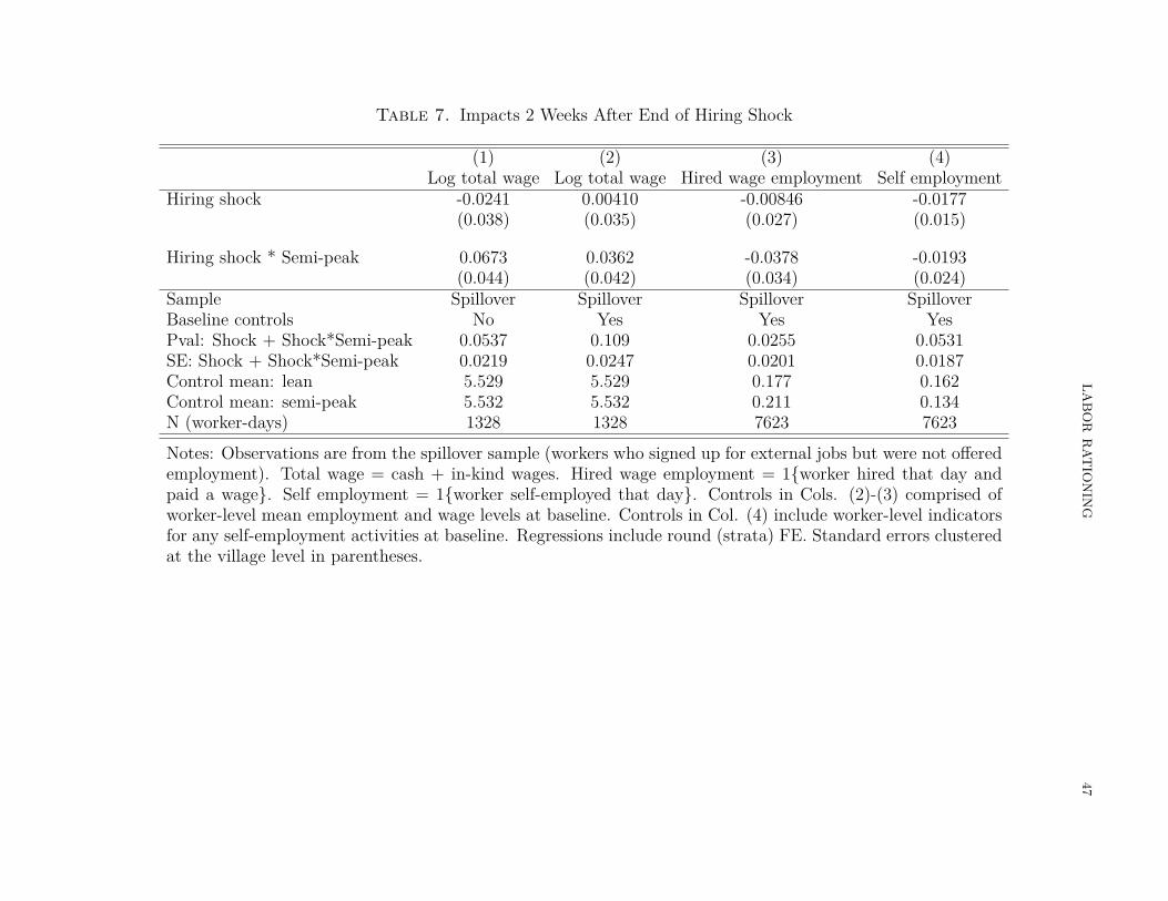
LAB

OR

RAT

ION

ING

47

Table 7. Impacts 2 Weeks After End of Hiring Shock

(1) (2) (3) (4)Log total wage Log total wage Hired wage employment Self employment

Hiring shock -0.0241 0.00410 -0.00846 -0.0177(0.038) (0.035) (0.027) (0.015)

Hiring shock * Semi-peak 0.0673 0.0362 -0.0378 -0.0193(0.044) (0.042) (0.034) (0.024)

Sample Spillover Spillover Spillover SpilloverBaseline controls No Yes Yes YesPval: Shock + Shock*Semi-peak 0.0537 0.109 0.0255 0.0531SE: Shock + Shock*Semi-peak 0.0219 0.0247 0.0201 0.0187Control mean: lean 5.529 5.529 0.177 0.162Control mean: semi-peak 5.532 5.532 0.211 0.134N (worker-days) 1328 1328 7623 7623

Notes: Observations are from the spillover sample (workers who signed up for external jobs but were not offeredemployment). Total wage = cash + in-kind wages. Hired wage employment = 1{worker hired that day andpaid a wage}. Self employment = 1{worker self-employed that day}. Controls in Cols. (2)-(3) comprised ofworker-level mean employment and wage levels at baseline. Controls in Col. (4) include worker-level indicatorsfor any self-employment activities at baseline. Regressions include round (strata) FE. Standard errors clusteredat the village level in parentheses.

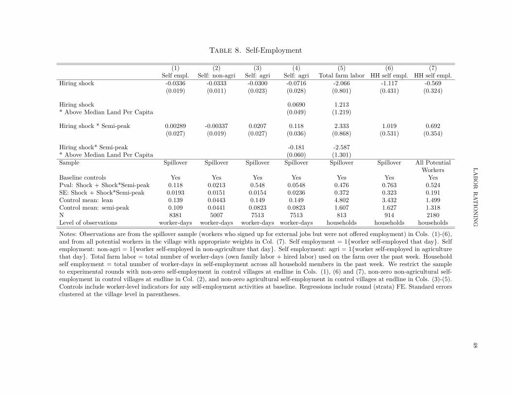
LAB

OR

RAT

ION

ING

48

Table 8. Self-Employment

(1) (2) (3) (4) (5) (6) (7)Self empl. Self: non-agri Self: agri Self: agri Total farm labor HH self empl. HH self empl.

Hiring shock -0.0336 -0.0333 -0.0300 -0.0716 -2.066 -1.117 -0.569(0.019) (0.011) (0.023) (0.028) (0.801) (0.431) (0.324)

Hiring shock 0.0690 1.213* Above Median Land Per Capita (0.049) (1.219)

Hiring shock * Semi-peak 0.00289 -0.00337 0.0207 0.118 2.333 1.019 0.692(0.027) (0.019) (0.027) (0.036) (0.868) (0.531) (0.354)

Hiring shock* Semi-peak -0.181 -2.587* Above Median Land Per Capita (0.060) (1.301)Sample Spillover Spillover Spillover Spillover Spillover Spillover All Potential

WorkersBaseline controls Yes Yes Yes Yes Yes Yes YesPval: Shock + Shock*Semi-peak 0.118 0.0213 0.548 0.0548 0.476 0.763 0.524SE: Shock + Shock*Semi-peak 0.0193 0.0151 0.0154 0.0236 0.372 0.323 0.191Control mean: lean 0.139 0.0443 0.149 0.149 4.802 3.432 1.499Control mean: semi-peak 0.109 0.0441 0.0823 0.0823 1.607 1.627 1.318N 8381 5007 7513 7513 813 914 2180Level of observations worker-days worker-days worker-days worker-days households households households

Notes: Observations are from the spillover sample (workers who signed up for external jobs but were not offered employment) in Cols. (1)-(6),and from all potential workers in the village with appropriate weights in Col. (7). Self employment = 1{worker self-employed that day}. Selfemployment: non-agri = 1{worker self-employed in non-agriculture that day}. Self employment: agri = 1{worker self-employed in agriculturethat day}. Total farm labor = total number of worker-days (own family labor + hired labor) used on the farm over the past week. Householdself employment = total number of worker-days in self-employment across all household members in the past week. We restrict the sampleto experimental rounds with non-zero self-employment in control villages at endline in Cols. (1), (6) and (7), non-zero non-agricultural self-employment in control villages at endline in Col. (2), and non-zero agricultural self-employment in control villages at endline in Cols. (3)-(5).Controls include worker-level indicators for any self-employment activities at baseline. Regressions include round (strata) FE. Standard errorsclustered at the village level in parentheses.

LAB

OR

RAT

ION

ING

49

Table 9. Measuring Involuntary Unemployment

(1) (2) (3) (4) (5) (6)Any Any Invol unempl Invol unempl Invol unempl Invol unemplwork work (traditional) (traditional) (alternate) alternate)

Hiring shock 0.0222 0.0153 -0.0385 -0.0322 -0.0699 -0.0611(0.028) (0.023) (0.028) (0.027) (0.026) (0.026)

Hiring shock * Semi-peak -0.0264 -0.0282 0.0296 0.0300 0.0638 0.0647(0.035) (0.029) (0.039) (0.038) (0.039) (0.038)

Sample Spillover Spillover Spillover Spillover Spillover SpilloverBaseline controls No Yes No Yes No YesPval: Shock + Shock*Semi-peak 0.842 0.477 0.741 0.932 0.837 0.900SE: Shock + Shock*Semi-peak 0.0207 0.0181 0.0267 0.0260 0.0297 0.0285Control mean: lean 0.341 0.341 0.482 0.482 0.580 0.580Control mean: semi-peak 0.398 0.398 0.395 0.395 0.540 0.540N (worker-days) 8906 8906 8906 8906 8906 8906

Notes: Observations are from the spillover sample (workers who signed up for external jobs but were not offered em-ployment). Any work = 1{worker reports any work that day}. Involuntary unemployment (traditional) = 1{workerreports “would have liked to work but was unable to find any” as his activity status for that day}. Involuntary un-employment (alternate) = 1{worker states that they would have accepted a job at the prevailing wage over whateverelse they had been doing that day}. Controls include worker-level mean employment and wage levels at baseline.Regressions include round (strata) FE. Standard errors clustered at the village level in parentheses. Test comparingthe coefficients in Cols. 3 vs. 5: p-val = 0.0674. Test comparing the coefficients in Cols. 4 vs. 6: p-val = 0.1147.

LABOR RATIONING 50

FOR ONLINE PUBLICATION

Appendix A. Appendix Figures

Wage

Village EmplE

w

S

D

D′(treatment)

E ′

w′

text to align

(a) H0 : No Rationing (ED ≥ ES)

Wage

Village Empl

S

D′(treatment)

D

E = ED ESE′D

w

Rationing

(b) H1 : Rationing (ED < ES)

Figure A.1. Effects of a Negative Labor Demand Shock

Note: Figure shows the effects of a negative demand shock on employmentand wages under no rationing (ED ≥ ES) in panel A, and under rationing(ED < ES) in panel B.

LABOR RATIONING 51

Wage

EmploymentMRPL

S

MCL

E′E

w′w

Figure A.2. Effects of a Negative Labor Supply Shock Under Monopsony

Note: Figure shows the effects of a negative supply shock on employment andwages under monopsony. A parallel shift in labor supply leads wages to riseand employment to fall, the same qualitative predictions as in the benchmark,market clearing model. Because the marginal cost of labor curve is steeper thanthe labor supply curve, the wage increases by less and employment decreasesby more under monopsony, relative to market clearing.

0.0

5.1

.15

.2.2

5.3

Aver

age

Hire

d W

age

Empl

oym

ent

Jan. Feb. Mar. Apr. May. Jun. Jul. Aug. Sep. Oct. Nov. Dec.

Figure A.3. Average Hired Wage Employment Rate by Month

Note: Figure plots average wage employment rates in control villages by cal-endar month. The median employment rate is 0.19.

LABOR RATIONING 52

02

46

Labo

r use

per

acr

e

0 1 2 3 4Acres

95% CI lpoly smoothkernel = epanechnikov, degree = 2, bandwidth = .81, pwidth = 1.21

Figure A.4. Inverse Farm-Size Relationship

Note: Figure plots intensity of labor use against farm size. The y-axis measurestotal labor inputs per acre on the farm in the past week (own family labor +hired labor).

Figure A.5. Job take-up

Note: Figure illustrates take up of a job offer made in private at differentwage rates among casual workers in villages similar to our study sample, inthe same districts of Odisha, India. This data comes from a labor supplyestimation exercise conducted by Breza et al. (2019).

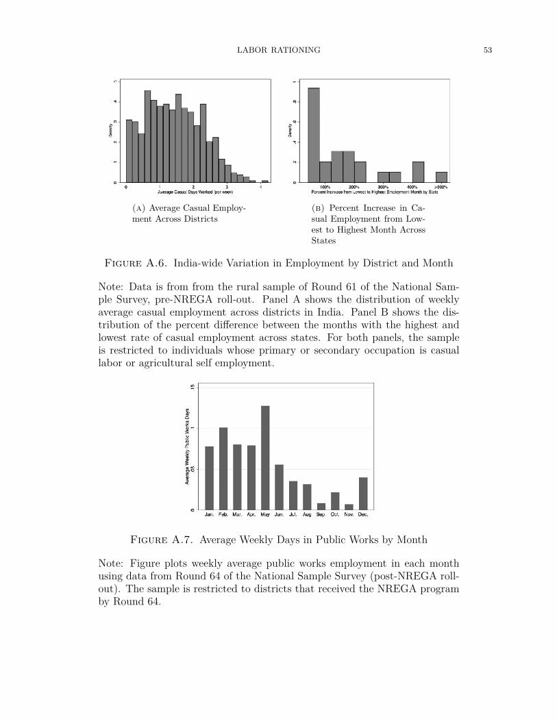
LABOR RATIONING 53

(a) Average Casual Employ-ment Across Districts

(b) Percent Increase in Ca-sual Employment from Low-est to Highest Month AcrossStates

Figure A.6. India-wide Variation in Employment by District and Month

Note: Data is from from the rural sample of Round 61 of the National Sam-ple Survey, pre-NREGA roll-out. Panel A shows the distribution of weeklyaverage casual employment across districts in India. Panel B shows the dis-tribution of the percent difference between the months with the highest andlowest rate of casual employment across states. For both panels, the sampleis restricted to individuals whose primary or secondary occupation is casuallabor or agricultural self employment.

Figure A.7. Average Weekly Days in Public Works by Month

Note: Figure plots weekly average public works employment in each monthusing data from Round 64 of the National Sample Survey (post-NREGA roll-out). The sample is restricted to districts that received the NREGA programby Round 64.

LABOR RATIONING 54

Appendix B. Appendix TablesTable B.1. Survey Completion in Spillover Sample

(1) (2)Baseline Survey Completion Endline Survey Completion

Hiring shock 0.0160 0.0125(0.019) (0.014)

Sample Spillover SpilloverDep Var Mean 0.934 0.896N (workers) 1094 1108

Notes: Observations are from the spillover sample (workers who signed upfor external jobs but were not offered employment). The dependent vari-able is a binary indicator for whether the survey respondent completed thesurvey. Col. (1) examines baseline survey responses and Col. (2) examinesendline survey responses. Regressions include round (strata) FEs. Theregression in Col. (2) includes a control for baseline survey completion.Standard errors are clustered at the village level in parentheses.

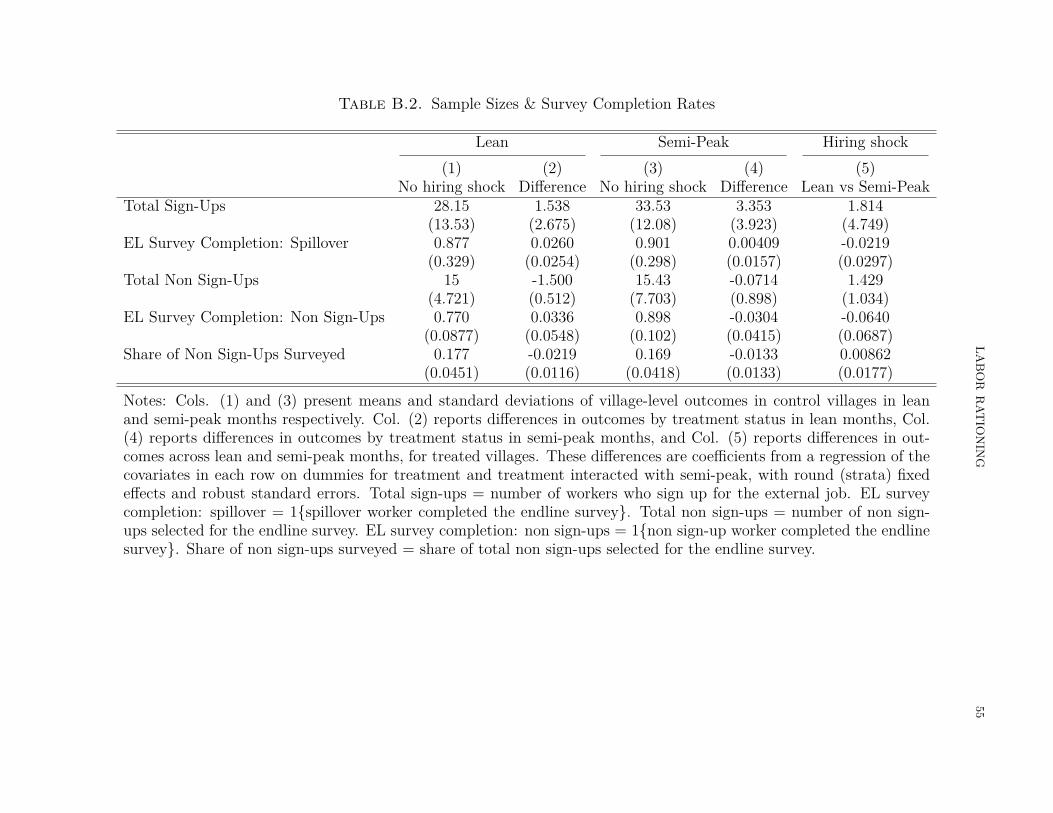
LAB

OR

RAT

ION

ING

55

Table B.2. Sample Sizes & Survey Completion Rates

Lean Semi-Peak Hiring shock(1) (2) (3) (4) (5)

No hiring shock Difference No hiring shock Difference Lean vs Semi-PeakTotal Sign-Ups 28.15 1.538 33.53 3.353 1.814

(13.53) (2.675) (12.08) (3.923) (4.749)EL Survey Completion: Spillover 0.877 0.0260 0.901 0.00409 -0.0219

(0.329) (0.0254) (0.298) (0.0157) (0.0297)Total Non Sign-Ups 15 -1.500 15.43 -0.0714 1.429

(4.721) (0.512) (7.703) (0.898) (1.034)EL Survey Completion: Non Sign-Ups 0.770 0.0336 0.898 -0.0304 -0.0640

(0.0877) (0.0548) (0.102) (0.0415) (0.0687)Share of Non Sign-Ups Surveyed 0.177 -0.0219 0.169 -0.0133 0.00862

(0.0451) (0.0116) (0.0418) (0.0133) (0.0177)

Notes: Cols. (1) and (3) present means and standard deviations of village-level outcomes in control villages in leanand semi-peak months respectively. Col. (2) reports differences in outcomes by treatment status in lean months, Col.(4) reports differences in outcomes by treatment status in semi-peak months, and Col. (5) reports differences in out-comes across lean and semi-peak months, for treated villages. These differences are coefficients from a regression of thecovariates in each row on dummies for treatment and treatment interacted with semi-peak, with round (strata) fixedeffects and robust standard errors. Total sign-ups = number of workers who sign up for the external job. EL surveycompletion: spillover = 1{spillover worker completed the endline survey}. Total non sign-ups = number of non sign-ups selected for the endline survey. EL survey completion: non sign-ups = 1{non sign-up worker completed the endlinesurvey}. Share of non sign-ups surveyed = share of total non sign-ups selected for the endline survey.

LAB

OR

RAT

ION

ING

56

Table B.3. Baseline Characteristics: Sign-Ups and Non Sign-Ups

Lean Semi-Peak(1) (2) (3) (4) (5) (6)

Sign-Ups Difference pval Sign-Ups Difference pvalEver participate in casual labor market 1 -0.149 0.0321 0.986 -0.215 0.000788

(0.000) (0.061) (0.118) (0.052)Days would like to work in labor market (in next 30 days) 16.60 -4.707 0.0268 19.10 -6.517 0.00366

(9.005) (1.843) (8.079) (1.917)Total wage (Rs.) 254.6 31.27 0.0135 251.2 8.708 0.254

(67.723) (10.202) (56.468) (7.347)Weekly wage earnings 675.4 23.96 0.804 637.7 -20.73 0.787

(514.302) (94.285) (545.994) (75.464)Any activity 0.389 0.0961 0.363 0.331 -0.0408 0.400

(0.367) (0.101) (0.352) (0.047)Employment rate: Hired wage employment 0.179 -0.0564 0.395 0.176 -0.0688 0.155

(0.282) (0.064) (0.288) (0.046)Public works employment 0.0124 0 1 0.000366 0 1

(0.093) (0.000) (0.007) (0.000)Has HH business 0.859 -0.0213 0.754 0.890 -0.0385 0.0853

(0.348) (0.066) (0.313) (0.021)Self employment 0.164 0.0597 0.156 0.0874 0.0283 0.120

(0.281) (0.039) (0.216) (0.017)Landless 0.506 -0.116 0.0196 0.295 -0.0289 0.401

(0.501) (0.043) (0.457) (0.034)HH members (age 12+) 3.988 -0.143 0.486 3.952 -0.175 0.189

(1.696) (0.198) (1.422) (0.128)Social category: Scheduled caste/tribe 0.817 -0.0433 0.594 0.752 -0.166 0.0424

(0.388) (0.076) (0.433) (0.070)

Notes: Cols. (1) and (4) present baseline means and standard deviations of worker-level characteristics in control villages forworkers who sign up for external jobs in lean and semi-peak months respectively. Cols. (2) and (5) report coefficients fromregressing the covariate in each row on a dummy for non sign-ups in lean and semi-peak months respectively, with round(strata) fixed effects and standard errors clustered at the village level. Cols. (3) and (6) report corresponding p-values forthe regression coefficients presented in Cols. (2) and (5) respectively.

LAB

OR

RAT

ION

ING

57

Table B.4. Wage Effects using Non-Winsorized Wages

(1) (2) (3) (4) (5) (6)Log cash wage Log total wage Log total wage Total wage Log total wage Total wage

Hiring shock -0.0202 -0.0113 -0.0183 -5.632 -0.0620 -19.24(0.021) (0.022) (0.019) (3.925) (0.050) (11.425)

Hiring shock * Semi-peak 0.0740 0.0676 0.0684 18.57(0.031) (0.032) (0.029) (7.595)

Hiring Shock * Empl. Level 0.457 133.3(0.240) (57.182)

Sample Spillover Spillover Spillover Spillover Spillover SpilloverBaseline controls No No Yes Yes Yes YesPval: Shock + Shock*Semi-peak 0.0232 0.0227 0.0256 0.0472 . .SE: Shock + Shock*Semi-peak 0.0231 0.0241 0.0219 6.379 . .Control mean: lean 5.458 5.500 5.500 253.8 5.500 253.8Control mean: semi-peak 5.428 5.504 5.504 251.6 5.504 251.6N (worker-days) 1543 1544 1544 1545 1544 1545

Notes: Observations are from the spillover sample (workers who signed up for external jobs but were not offered employment).Total wage = cash + in-kind wages. Controls include worker-level mean employment and wage levels at baseline. Regressionsinclude round (strata) FEs. Standard errors are clustered at the village level in parentheses.

LAB

OR

RAT

ION

ING

58

Table B.5. Treatment Effects Restricting to 7-day Recall Window

(1) (2) (3) (4) (5) (6)Hired wage empl. Log total wage Self empl. Hired wage empl. Log total wage Self empl.

Hiring shock 0.0518 -0.00613 -0.0534 0.00530 0.00616 -0.00282(0.023) (0.015) (0.018) (0.031) (0.036) (0.017)

Hiring shock * Semi-peak -0.0855 0.0450 0.0260 -0.0658 0.0247 -0.0236(0.032) (0.028) (0.025) (0.038) (0.044) (0.025)

Sample Spillover Spillover Spillover Spillover Spillover SpilloverBaseline controls Yes Yes Yes Yes Yes YesPval: Shock + Shock*Semi-peak 0.140 0.0948 0.150 0.00764 0.230 0.159SE: Shock + Shock*Semi-peak 0.0226 0.0229 0.0188 0.0218 0.0254 0.0185Control mean: lean 0.156 5.526 0.171 0.188 5.543 0.174Control mean: semi-peak 0.232 5.502 0.107 0.222 5.529 0.130N (worker-days) 6944 1274 6545 6196 1131 6196

Notes: Observations are from the spillover sample (workers who signed up for external jobs but were not offered employment).Hired wage employment = 1{worker hired that day and paid a wage}. Total wage = cash + in-kind wages. Self employment =1{worker self-employed that day}. Cols. (4) to (6) examine impacts two weeks after the end of the hiring shock. Regressionsinclude round (strata) FEs. Standard errors are clustered at the village level in parentheses.

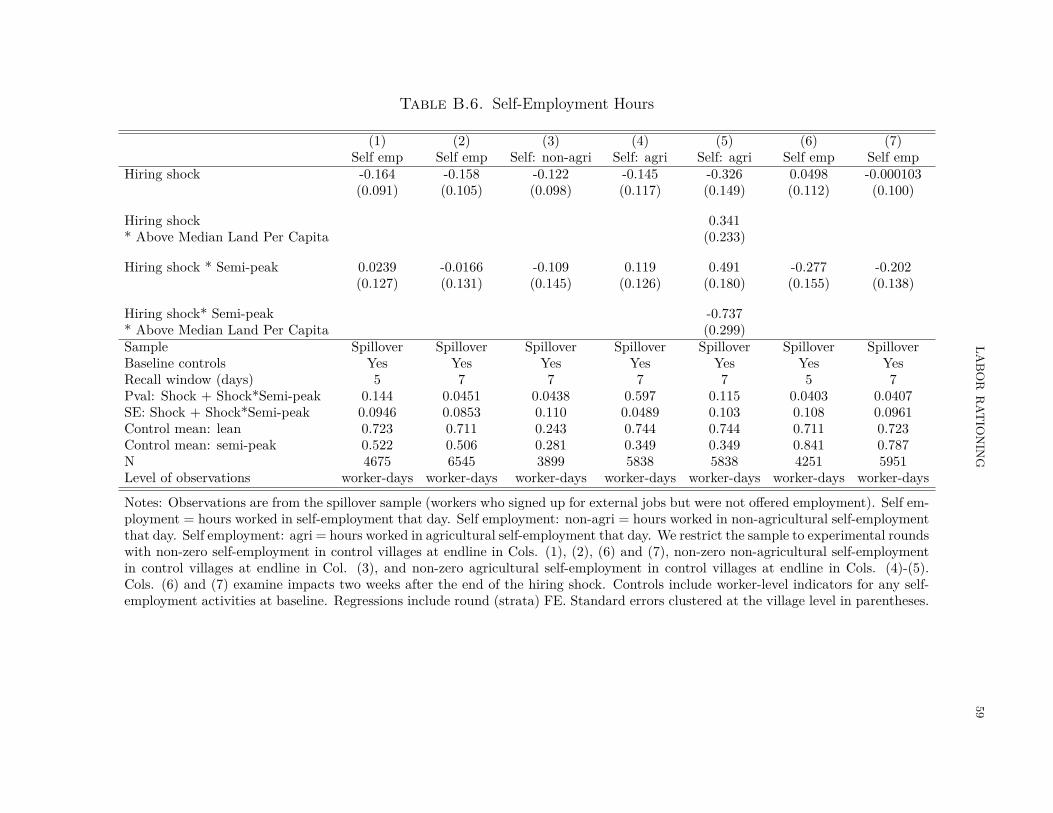
LAB

OR

RAT

ION

ING

59

Table B.6. Self-Employment Hours

(1) (2) (3) (4) (5) (6) (7)Self emp Self emp Self: non-agri Self: agri Self: agri Self emp Self emp

Hiring shock -0.164 -0.158 -0.122 -0.145 -0.326 0.0498 -0.000103(0.091) (0.105) (0.098) (0.117) (0.149) (0.112) (0.100)

Hiring shock 0.341* Above Median Land Per Capita (0.233)

Hiring shock * Semi-peak 0.0239 -0.0166 -0.109 0.119 0.491 -0.277 -0.202(0.127) (0.131) (0.145) (0.126) (0.180) (0.155) (0.138)

Hiring shock* Semi-peak -0.737* Above Median Land Per Capita (0.299)Sample Spillover Spillover Spillover Spillover Spillover Spillover SpilloverBaseline controls Yes Yes Yes Yes Yes Yes YesRecall window (days) 5 7 7 7 7 5 7Pval: Shock + Shock*Semi-peak 0.144 0.0451 0.0438 0.597 0.115 0.0403 0.0407SE: Shock + Shock*Semi-peak 0.0946 0.0853 0.110 0.0489 0.103 0.108 0.0961Control mean: lean 0.723 0.711 0.243 0.744 0.744 0.711 0.723Control mean: semi-peak 0.522 0.506 0.281 0.349 0.349 0.841 0.787N 4675 6545 3899 5838 5838 4251 5951Level of observations worker-days worker-days worker-days worker-days worker-days worker-days worker-days

Notes: Observations are from the spillover sample (workers who signed up for external jobs but were not offered employment). Self em-ployment = hours worked in self-employment that day. Self employment: non-agri = hours worked in non-agricultural self-employmentthat day. Self employment: agri = hours worked in agricultural self-employment that day. We restrict the sample to experimental roundswith non-zero self-employment in control villages at endline in Cols. (1), (2), (6) and (7), non-zero non-agricultural self-employmentin control villages at endline in Col. (3), and non-zero agricultural self-employment in control villages at endline in Cols. (4)-(5).Cols. (6) and (7) examine impacts two weeks after the end of the hiring shock. Controls include worker-level indicators for any self-employment activities at baseline. Regressions include round (strata) FE. Standard errors clustered at the village level in parentheses.

LAB

OR

RAT

ION

ING

60

Table B.7. Self-Employment

(1) (2) (3)Self empl: Self empl: Total Farmnon-agri agri Labor

Hiring shock -0.0351 -0.0925 -1.940(0.008) (0.038) (0.726)

Hiring shock 0.172 1.971* Above Median Land Per Capita (0.064) (0.903)

Hiring shock * Semi-peak 0.00703 0.155 2.883(0.013) (0.043) (0.811)

Hiring shock * Semi-peak -0.228 -2.948* Above Median Land Per Capita (0.073) (1.037)Sample All Potential All Potential All Potential

Workers Workers WorkersBaseline controls Yes Yes YesPval: Shock + Shock*Semi-peak 0.0314 0.00562 0.0234SE: Shock + Shock*Semi-peak 0.0125 0.0217 0.402Control mean: lean 0.0303 0.151 3.408Control mean: semi-peak 0.0589 0.0817 1.582N 11662 17774 1928Level of observations worker-days worker-days households

Notes: Observations are from all potential workers in the village with appro-priate weights. Self employment: non-agri = 1{worker self-employed in non-agriculture that day}. Self employment: agri = 1{worker self-employed in agri-culture that day}. Total farm labor = total number of worker-days (own familylabor + hired labor) used on the farm over the past week. Controls includeworker-level indicators for any self-employment activities at baseline. Regres-sions include round (strata) FE. Standard errors clustered at the village levelin parentheses.

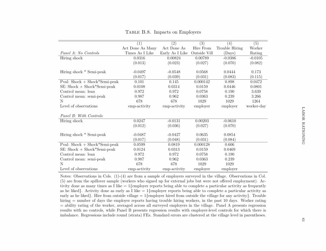
LAB

OR

RAT

ION

ING

61

Table B.8. Impacts on Employers

(1) (2) (3) (4) (5)Act Done As Many Act Done As Hire From Trouble Hiring Worker

Panel A: No Controls Times As I Like Early As I Like Outside Vill (Days) RatingHiring shock 0.0316 0.00824 0.00789 -0.0386 -0.0105

(0.013) (0.023) (0.027) (0.070) (0.082)

Hiring shock * Semi-peak -0.0497 -0.0548 0.0568 0.0444 0.173(0.017) (0.039) (0.031) (0.083) (0.115)

Pval: Shock + Shock*Semi-peak 0.101 0.145 0.000142 0.898 0.0472SE: Shock + Shock*Semi-peak 0.0108 0.0314 0.0159 0.0446 0.0801Control mean: lean 0.972 0.972 0.0758 0.190 3.639Control mean: semi-peak 0.987 0.962 0.0363 0.239 3.266N 678 678 1029 1029 1264Level of observations emp-activity emp-activity employer employer worker-day

Panel B: With ControlsHiring shock 0.0247 -0.0131 0.00203 -0.0610

(0.012) (0.036) (0.027) (0.070)

Hiring shock * Semi-peak -0.0487 -0.0427 0.0635 0.0854(0.017) (0.048) (0.031) (0.084)

Pval: Shock + Shock*Semi-peak 0.0599 0.0819 0.000128 0.606SE: Shock + Shock*Semi-peak 0.0124 0.0313 0.0159 0.0469Control mean: lean 0.972 0.972 0.0758 0.190Control mean: semi-peak 0.987 0.962 0.0363 0.239N 678 678 1029 1029Level of observations emp-activity emp-activity employer employer

Notes: Observations in Cols. (1)-(4) are from a sample of employers surveyed in the village. Observations in Col.(5) are from the spillover sample (workers who signed up for external jobs but were not offered employment). Ac-tivity done as many times as I like = 1{employer reports being able to complete a particular activity as frequentlyas he liked}. Activity done as early as I like = 1{employer reports being able to complete a particular activity asearly as he liked}. Hire from outside village = 1{employer hired from outside the village for any activity}. Troublehiring = number of days the employer reports having trouble hiring workers, in the past 10 days. Worker rating= ability rating of the worker, averaged across all surveyed employers in the village. Panel A presents regressionresults with no controls, while Panel B presents regression results with employer-level controls for which there isimbalance. Regressions include round (strata) FEs. Standard errors are clustered at the village level in parentheses.

LAB

OR

RAT

ION

ING

62

Table B.9. Employment Spillovers: Heterogeneous Impacts by Ability

Dependent variable: Hired wage employment

High ability proxy(1) (2) (3)

Employer Rating Employment Rate WagesHiring shock 0.0847 0.0526 0.0628

(0.022) (0.018) (0.018)

Hiring shock * Semi-peak -0.103 -0.0662 -0.0780(0.040) (0.029) (0.031)

High ability proxy 0.0246 0.0752 0.0521(0.018) (0.018) (0.013)

Hiring Shock* High ability proxy -0.00450 -0.0441 -0.00906(0.030) (0.030) (0.025)

Semi-peak* High ability proxy -0.0139 0.0470 0.0644(0.023) (0.024) (0.024)

Hiring shock* Semi-peak* High ability proxy 0.0309 0.0495 0.00975(0.035) (0.041) (0.039)

Sample Spillover Spillover SpilloverBaseline controls No No NoPval: Shock + Shock*Semi-peak 0.586 0.540 0.548SE: Shock + Shock*Semi-peak 0.0334 0.0221 0.0253Control mean: lean 0.134 0.145 0.145Control mean: semi-peak 0.228 0.216 0.216N (worker-days) 6405 8906 8906

Notes: Observations are from the spillover sample (workers who signed up for external jobsbut were not offered employment). We use three different worker-level proxies for high ability:standardized quality rating averaged across all survey employers in the village in Col.(1), stan-dardized mean employment levels at baseline in Col. (2), and standardized mean wage levels atbaseline in Col. (3). Regressions include round (strata) FEs. Standard errors are clustered atthe village level in parentheses.

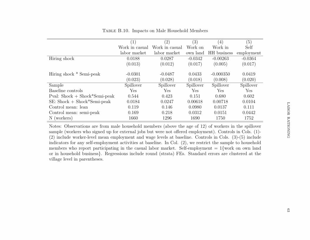
LAB

OR

RAT

ION

ING

63

Table B.10. Impacts on Male Household Members

(1) (2) (3) (4) (5)Work in casual Work in casual Work on Work in Selflabor market labor market own land HH business employment

Hiring shock 0.0188 0.0287 -0.0342 -0.00263 -0.0364(0.013) (0.012) (0.017) (0.005) (0.017)

Hiring shock * Semi-peak -0.0301 -0.0487 0.0433 -0.000350 0.0419(0.023) (0.028) (0.018) (0.008) (0.020)

Sample Spillover Spillover Spillover Spillover SpilloverBaseline controls Yes Yes Yes Yes YesPval: Shock + Shock*Semi-peak 0.544 0.423 0.151 0.680 0.602SE: Shock + Shock*Semi-peak 0.0184 0.0247 0.00618 0.00718 0.0104Control mean: lean 0.119 0.146 0.0980 0.0137 0.111Control mean: semi-peak 0.169 0.218 0.0312 0.0151 0.0442N (workers) 1660 1296 1690 1750 1752

Notes: Observations are from male household members (above the age of 12) of workers in the spilloversample (workers who signed up for external jobs but were not offered employment). Controls in Cols. (1)-(2) include worker-level mean employment and wage levels at baseline. Controls in Cols. (3)-(5) includeindicators for any self-employment activities at baseline. In Col. (2), we restrict the sample to householdmembers who report participating in the casual labor market. Self-employment = 1{work on own landor in household business}. Regressions include round (strata) FEs. Standard errors are clustered at thevillage level in parentheses.

LAB

OR

RAT

ION

ING

64

Table B.11. Differential Impacts of NREGS by Labor Market Slack

(1) (2) (3) (4) (5)Public Works Casual Casual Days Casual Agri. Self-Empl.

Days Wage Worked Days DaysNREGA 0.0213 -0.618 0.0678 -0.00650 -0.206

(0.010) (1.009) (0.054) (0.047) (0.071)

NREGA x High Casual Employment 0.00906 2.594 -0.0980 -0.121 0.0923(0.013) (1.052) (0.059) (0.061) (0.080)

Control Mean 0.0121 72.00 1.071 0.652 4.738Test: NREGA + NREGA x High Cas. Empl. 0.0132 0.0554 0.609 0.0308 0.152Observations 353180 64634 353180 353180 329177

Notes: Observations are from prime-age individuals surveyed in rounds 61 and 64 of Schedule 10 of the NationalSample Survey (NSS), with sampling weights. Regressions include district and month-by-year fixed effects, aswell as a vector of controls including worker characteristics by round (gender, education, age), baseline agricul-tural yields by round, and district-by-month baseline means of casual employment, wages, and self-employment.Standard errors are clustered at the district level in parentheses.

LAB

OR

RAT

ION

ING

65

Table B.12. Treatment Effects Using All Experimental Rounds

(1) (2) (3) (4) (5) (6)Log total Hired wage Hired wage Self Invol unempl Invol unempl

wage employment employment employment (traditional) (alternate)Hiring shock -0.0181 0.0540 0.0101 -0.0331 -0.0339 -0.0625

(0.019) (0.018) (0.022) (0.019) (0.027) (0.026)

Hiring shock * Semi-peak 0.0673 -0.0681 -0.0551 -0.00737 0.0529 0.0793(0.028) (0.028) (0.025) (0.026) (0.037) (0.037)

Sample Spillover Spillover All Workers Spillover Spillover SpilloverBaseline controls Yes Yes Yes Yes Yes YesPval: Shock + Shock*Semi-peak 0.0189 0.526 0.000629 0.0263 0.453 0.523SE: Shock + Shock*Semi-peak 0.0204 0.0221 0.0125 0.0178 0.0252 0.0262Control mean: lean 5.500 0.145 0.135 0.139 0.482 0.580Control mean: semi-peak 5.502 0.209 0.185 0.112 0.413 0.553N (worker-days) 1603 9466 22398 8941 9466 9466

Notes: This table presents regression results including two experimental rounds that were excluded from the mainanalysis because we were not able to complete survey work (see Appendix C). Observations in Cols. (1)-(2) and(4)-(6) are from the spillover sample (workers who signed up for external jobs but were not offered employment).Observations in Col. (3) are from all potential workers in the village with appropriate weights. Controls in Cols.(1)-(2) and (5)-(6) include worker-level mean employment and wage levels at baseline. Controls in Col. (3) includeworker-level and village-level mean employment and wage levels at baseline. Controls in Col. (4) include indicatorsfor any self-employment activities at baseline. Regressions include round (strata) FEs. Standard errors clustered atthe village level in parentheses.

LAB

OR

RAT

ION

ING

66

Table B.13. Employer Characteristics

Lean Semi-Peak(1) (2) (3) (4) (5) (6)

No hiring shock Difference Pval No hiring shock Difference PvalLandholdings (acres) 2.634 0.308 0.0947 2.631 -0.0506 0.645

(1.696) (0.177) (1.696) (0.109)HH members (age 12+) 4.199 0.178 0.167 4.254 0.265 0.0258

(1.508) (0.124) (1.508) (0.114)Fraction of randomly selected workers given a rating 0.725 -0.0151 0.702 0.791 0.0366 0.209

(0.250) (0.039) (0.250) (0.029)Fraction of randomly selected workers ever hired 0.257 0.00727 0.817 0.216 0.0116 0.473

(0.221) (0.031) (0.221) (0.016)Ever participate in casual labor market 0.569 -0.0488 0.266 0.495 -0.000666 0.985

(0.496) (0.043) (0.496) (0.035)Occupation: Self-emp (agri) 0.611 -0.0208 0.123 0.620 -0.0176 0.00702

(0.489) (0.013) (0.489) (0.006)Occupation: Self-emp (non-agri) 0.0616 -0.0191 0.316 0.0693 -0.00483 0.718

(0.241) (0.019) (0.241) (0.013)Occupation: Laborer 0.303 -0.0556 0.192 0.274 -0.0197 0.463

(0.461) (0.041) (0.461) (0.026)Social category: Scheduled caste/tribe 0.332 -0.175 0.000572 0.281 -0.0300 0.444

(0.472) (0.044) (0.472) (0.039)

Notes: Observations are from the employer survey. Cols. (1) and (4) present means and standard deviations of employer-level char-acteristics in control villages in lean and semi-peak months respectively. Cols. (2) and (5) report coefficients from regressing thecovariate in each row on a dummy for treatment in lean and semi-peak months respectively, with round (strata) fixed effects andstandard errors clustered at the village level. Cols. (3) and (6) report corresponding p-values for the regression coefficients presentedin Cols. (2) and (5) respectively.

LABOR RATIONING 67

Appendix C. Implementation Protocols

Recruitment of study participants. Several days prior to the first day of work, the externaljobs are advertised in villages through flyers, village meetings, and door-to-door visits. First,flyers containing basic information about the job opportunity (nature of work, duration,hours per day, location, daily wage etc.) are distributed to all households. Next, a meetingis held in a central location within the village. During this meeting, more information is givento interested workers. For example, they are informed that the job opportunity is one-timeonly and employment is not guaranteed — the number of workers hired would depend on theneeds of local contractors, and job offers would be randomly assigned among those who signup using a lottery.45 Lastly, door-to-door visits are made to ensure that all households in thevillage have received information about the external job opportunity. Male workers who areinterested in the job are encouraged to sign up at the village meeting or during door-to-doorvisits. Workers who are under the age of 18 or above the age of 65 are ineligible.

We use a computer to randomize assignment of eligible sign-ups to one of three groups: (1)workers who will be offered a job; (2) workers who might be offered a job (waitlist); and(3) workers who will never be offered a job. We draw from the group 2 roster in the eventthat a worker from group 1 opts out of the external job. Workers in group 3 constitutes ourspillover sample.

Description of external jobs. The external jobs take place in factory workshops within 15kilometers of our study villages. Workers are employed full-time (5 days a week) for 2-4 weeks,and they engage in low-skill manufacturing of products such as ropes, brooms, disposableplates and floor mats. All output produced by workers is sold by partnering contractors, whoset production standards. Workers are paid a flat daily wage for attendance, in accordancewith the typical pay structure in the area. There are no strict production minimums imposedon workers, though workers can be fired for excessive absences (more than three days in arow) or disruptive behavior.

At any point in time, a total of approximately 30 workers are recruited into a worksite —this comprises of workers from both treatment and control villages within an experimentalround. In experimental rounds where the number of recruited workers across both treatmentand control villages is less than 30, we hire additional workers from nearby villages until wereach the capacity limit at the factory workshop.

More details on the external jobs can be found in Breza et al. (2018).45We advertise the jobs as “training contracts,” indicating that workers will receive one-time training toproduce a low-skill manufacturing good during their employment period. This concept is familiar in thiscontext, and is viewed as a one-time opportunity since one would not receive training more than once. SeeBreza et al. (2018) for further details.

LABOR RATIONING 68

Worker surveys. We conduct surveys with all eligible workers who sign up. We also conductsurveys with a random sample of potential workers in the village who do not sign up for thejob. For this sample, the enumerators follow a left-hand rule — they start at the first house-hold on the left as they enter the village, and approach every three households thereafter.The survey is conducted with a prime-age male household member who is working in anycapacity — this includes work in the casual labor market, self-employment or salaried work.If a member of the household is part of the spillover sample, the household is skipped.

Timeline of worker surveys. We conduct three waves of surveys: (1) baseline surveys at thestart of the hiring shock; (2) endline surveys during the final two weeks of the hiring shock;and (3) post-intervention surveys two weeks after the end of the hiring shock.46 Surveys areconducted privately with workers at their residence. To compensate workers for their timeas well as to minimize survey attrition, workers are given a small gift upon completion ofthe post-intervention survey.

A subset of baseline surveys were conducted immediately after the external jobs began.Recall that in each of the surveys, workers are asked to describe their employment activityseparately for each day for the past 10 days. As such, part of the employment recall in thosesurveys included days during which the external job had already commenced. We restrictbaseline data used in regressions to worker-days that occurred before the external jobs began.As we document in the paper, our wage and employment effects are similar with or withoutbaseline controls.

Changes to worker survey instruments. In the first 9 experimental rounds, we collected recalldata for the past 14 days. We shortened this to 10 days for the next 9 rounds, and furthershortened this to 7 days for the remaining rounds.

As mentioned above, we began conducting the post-intervention worker survey in experimen-tal round 3. For the first six rounds thereafter, the survey was conducted 1-2 months afterthe end of the hiring shock. We shortened this to two weeks for the remaining experimentalrounds.

Employer surveys. In addition to worker surveys, we survey a subset of agricultural employersin the village at endline (i.e. during the final two weeks of the hiring shock). Our enumeratorsfirst consult a village resident to obtain a (partial) list of employers who hire agriculturalworkers in each village. Using this listing, we generate a roster with a randomized orderingof employers. Enumerators then conduct employer surveys following the order as stated inthe roster, with a stopping rule of 20 employer surveys per village. In some cases, there are46We added the post-intervention survey from experimental round 3 onwards.

LABOR RATIONING 69

fewer than 20 listed employers per village, so the total number of surveys completed is lessthan 20. The mean number of employer surveys completed per village is 18.

The employer survey includes a detailed hiring grid, in which employers describe each ac-tivity for which they required labor in the past 30 days. This includes data on labor use(number of workers, days worked, hiring location), cash wages and in-kind payments madeto hired workers for each activity, as well as whether the activity was completed as earlyand as frequently as they would have liked. All regressions using the employer sample areunweighted.

Changes to implementation protocols. In the last 11 experimental rounds, we conduct acensus of all households in our study villages prior to advertising the external job. Datafrom this census exercise allows us to:

(1) identify a random sample of potential workers in the village. We generate a rosterconsisting of prime-age males village residents who do not sign up for the job. Wedo not impose any condition on work status, as we did in earlier rounds.

(2) identify a sample of agricultural employers in the village. We generate a rosterconsisting of the five largest employers in the village (based on the number of worker-days they report hiring for a paid wage in the most recent harvest season), and arandom sampling of the remaining employers in the village.

This supersedes the protocol used to sample non-sign ups and agricultural employers outlinedabove.

Implementation issues. We faced issues conducting end line worker surveys in two experi-mental rounds and were only able to survey a small subset of intended participants. Onevillage previously had a negative experience with outsiders who promised gifts if the villageresidents converted to a particular religion. As such, residents in this village got suspicious(our standard survey protocol was to offer respondents a small gift upon completion of thesurveys) and refused to let our enumerators into the village to conduct surveys. In anothervillage, several village residents who were not part of our study sample did not want surveysto be conducted in their village. While the respondents themselves did not have any issuesparticipating in the survey, the hostility from other residents in the village made it difficultand potentially unsafe for our enumerators to enter the village. As such, we decided to haltdata collection in this village.

In Appendix Table B.12, we present regression results including the two experimental rounds,discussed here, that were excluded from the main analysis because we were not able tocomplete survey work. Our results are robust to the inclusion of these two rounds.

LABOR RATIONING 70

Appendix D. Construction of Census Variables

We use village-level data on demographic and economic indicators from the 2011 Indian Pop-ulation Census. This includes data on village size (population and number of households),caste composition, literacy, as well as worker counts.

As described in the 2011 Census meta data,47 workers are defined as “all persons (irrespectiveof age and sex) who participated in any economically productive activity for any length oftime during the reference period.” The reference period corresponds to the one year precedingthe date of survey enumeration. Workers who “worked for more than 6 months in thereference period” are referred to as main workers. Workers are further classified into fourcategories:

(1) agricultural laborers — this refers to individuals who “work on another person’s landfor wages in money or kind or share. She or he has no risk in the cultivation, butmerely works in another person’s land for wages”

(2) cultivators — this refers to individuals who are “engaged in cultivation of land ownedor held from Government or held from private persons or institutions for paymentsin money, kind or share”

(3) workers in household industry — household industry is defined as “an industry con-ducted by one or more members of the household at home or within the village inrural areas and only within the precincts of the house where the household lives inurban areas”

(4) other workers — this refers to workers other than those in categories (1)-(3). Exam-ples include work in the public sector, manufacturing, construction etc.

We construct several outcome variables using this data:

• Male population share: male population/village population• Literacy rate: literate population/village population• Worker share: all workers/village population• Male worker share: male workers/all workers• Main worker share: main workers/all workers• Agricultural labor share: agricultural laborers/all workers• Cultivator share: cultivators/all workers• Non-farm self-employment share: workers in household industry/all workers• Other workers share: other workers/all workers

47The 2011 Census meta data is available at https://www.censusindia.gov.in/2011census/HLO/Metadata_Census_2011.pdf.

LABOR RATIONING 71

Appendix E. Implied Aggregate Demand and Supply Elasticities

The nature of our shock allows us to back out both aggregate demand and supply elasticitiesduring semi-peak periods, if we are willing to assume competitive equilibrium. While thisis a strong assumption — and one that is not required in our main analysis — there arefew opportunities in the literature to measure these implied elasticities, so we include theseestimates here for completeness. Of course, as with all such analyses, the credibility ofthese estimates relies on the extent to which one believes in the underlying assumption ofcompetitive equilibrium in semi-peak times.

Wage

EmploymentEC

wC

ST

SC

D

∆h

∆w

∆e

∆w

∆h−∆e

ET

wT

Figure A.8. Aggregate Elasticities

Note: Figure illustrates how we can identify aggregate demand and supplyelasticities during semi-peak months, under the assumption of competitiveequilibrium. ∆w and ∆e denote the observed change in wages and employmentrespectively as a result of the hiring shock. The shock traces out the inverseslope of the demand curve, ∆e

∆w. ∆h denotes the size of the shift in aggregate

supply. Given ∆h, a simple geometric argument shows that the slope of thesupply curve is ∆w

∆h−∆e.

Appendix Figure A.8 shows how we can identify both the aggregate demand and supplyelasticities under this strong assumptions. We denote the observed change in wages betweentreatment and control as ∆w and the change in aggregate employment as ∆e. Given thatour treatment shifted the supply curve inward, the shock traces out the (inverse) slope of thedemand curve ∆e

∆w. That supply shocks identify demand elasticities is well known. However,

using arguments similar to Zoutman et al. (2018), we can also back out an implied supplyelasticity as well. Because we know the exact shock size—how many workers were employed

LABOR RATIONING 72

in our external jobs and those workers’ counterfactual employment rates—we can directlymeasure the size of the shift in aggregate supply ∆h.48 Given ∆h, a simple geometricargument shows that the inverse slope of the supply curve is ∆w

∆h−∆e.

Incorporating the impacts of our experimental shocks into this framework, the implied aggre-gate supply elasticity is 0.03, though clearly there is substantial noise around this estimate.This very small supply elasticity is consistent with the development literature.49 The impliedaggregate demand elasticity is -4.16, a very large magnitude relative to the literature.50 If webelieve that the magnitude of this implied demand elasticity is “too large,” then one of ourassumptions is likely unreasonable. First, under partially segmented markets, in semi-peakperiods, employers may substitute toward workers outside of the village, who typically com-mand higher wages. This would bias our measure of the change in employment in semi-peaktimes, leading to an overesimtate of the demand elasticity. Second, relaxing the assumptionof market clearing could also help to explain these large demand elasticity magnitudes. Onedeparture from market clearing that would yield an unbiased supply elasticity but distortthe implied demand elasticity is monopsony.51

In addition to the caveats about underlying assumptions, our estimates are measured withconsiderable noise. We consequently view them as suggestive. More generally, we intend thisstylized exercise to be illustrative—demonstrating how knowing the exact shock size enablesone to recover both elasticities with one source of variation.

48Recall that our experimental job paid workers a premium. Therefore ∆h is not equivalent to the fractionof laborers who took our job in treatment versus control, but instead the fraction of days they would haveworked at the market wage in absence of the external job.49For example, Goldberg (2016) measures a supply elasticity of 0.17 in rural Malawi.50The demand elasticity of Imbert and Papp (2020), obtained from a structural model of the migrationresponse to NREGA, is an imprecisely estimated -0.22. Kaur (2019)’s estimate is -1.17.51Under monopsony, employment levels are pinned down by the aggregate supply curve facing the employer.However, changes in employment and wages do not trace out the demand curve. In fact, wages fall by lessand employment falls by more under monopsony versus market clearing (Appendix Figure A.2), leading toan implied demand elasticity that is too large. This is consistent with the view of Muralidharan et al. (2020).