labor-market fluctuations and on-the-job...

LABOR-MARKET FLUCTUATIONS AND ON-THE-JOB SEARCH

ÉVA NAGYPÁL

Abstract. This paper argues that a model of the aggregate labor market that incorporates the

observed extent of job-to-job transitions can explain all the cyclical volatility in vacancy and unem-

ployment rates in U.S. data in response to shocks of the observed magnitude. The key to this result

is the complementarity between on-the-job search and costly hiring that leads employers to expect

a higher payo¤ from recruiting employed searchers. This higher expected payo¤ explains why �rms

recruit more when the number of employed searchers is high during periods of low unemployment.

Date: November, 2007.I would like to thank Paco Buera, Martin Eichenbaum, Robert Hall, Guido Menzio, Dale Mortensen, and GiorgioPrimiceri for their insightful suggestions. Many conference and seminar participants also provided valuable com-ments. All remaining errors are mine. and Department of Economics, Northwestern University, 2001 Sheridan Road,Evanston, IL 60208-2600, USA. E-mail: [email protected].

1

1. Introduction

The ongoing coexistence of unemployed workers and vacant positions has lent support in macro-

economics to a frictional view of labor markets wherein the matching of searching workers and

vacant positions takes time. According to this view, unemployment is low during boom periods

because there are many �rms recruiting and it takes little time for workers to become employed.

Recent research has suggested, however, that, in the context of a simple matching model, the ob-

served variation in the extent of recruitment cannot be understood as a response to changes in the

productivity and duration of prospective employment relationships (Shimer (2005), Mortensen and

Nagypál (2007b)). A critical question remains, namely, why do �rms recruit so much more in a

boom?

This paper o¤ers an answer to this question by arguing that workers search not only when un-

employed, but also while they are on a job. Due to the possibility of being able to stay with their

current employer, employed searchers are more selective in accepting job o¤ers than are unemployed

workers. They will only accept those jobs that are particularly attractive and that they are, there-

fore, unlikely to quit later on. This unique aspect makes the employment relationships formed by

employed searchers last longer than those formed by unemployed searchers amd allows a recruiting

�rm to recoup the cost of hiring over a longer period of time, thereby making it more pro�table for

�rms to recruit employed searchers.

In a matching model with on-the-job search, the higher pro�tability from recruiting employed

searchers leads to a multiplier e¤ect. When �rms recruit more, it is a good time for employed

workers to try and improve their lot by searching for a better job. In turn, when the pool of

searchers consists mostly of employed workers, it is a good time for �rms to recruit. This interplay

between recruitment and on-the-job search is empirically very important: the fraction of new jobs

that are �lled by workers who were employed immediately prior to starting their new jobs is around

one half and very strongly procyclical (Nagypál (2005b)). When I calibrate my model to match

this fact, the model can explain all the observed volatility in the vacancy and unemployment rates,

given a hiring cost of just over a week�s of wages.1

1These results signi�cantly improve upon those of Mortensen and Nagypál (2007b) whose calibrated matching modelwith the same features but without on-the-job search can explain only 52% of the volatility of the vacancy rate, akey endogenous variable in matching models.

2

It is important to emphasize that neither a hiring cost nor on-the-job search by itself could

generate the same amount of volatility. Rather, it is the interaction of the two that gives rise to my

results. Without including on-the-job search, not only does the model fail to account for the large

number of jobs �lled by previously employed searchers, it also explains only 62% of the observed

volatility in the vacancy rate. Without a hiring cost, the presence of on-the-job search actually

decreases ampli�cation so that the model can only explain 37% of the volatility of the vacancy rate.

In this case, it is more pro�table for �rms to recruit unemployed workers and the multiplier e¤ect

discussed above is absent.

Section 2 introduces my model of the labor market with on-the-job search and costly hiring.

Variation in the idiosyncratic job-satisfaction provided by di¤erent job matches leads to a desire

by workers to seek out more attractive and thereby longer lasting jobs and undertake job-to-job

transitions. In Section 3, I calibrate the model parameters to match the observed turnover in

the labor market, including the magnitude of job-to-job transitions. In Section 4, I highlight the

key mechanisms driving my results by characterizing a simpli�ed version of my model. I show

analytically that a higher pro�tability from recruiting employed searchers naturally arises in the

presence of costly hiring: the longer expected duration of matches formed with employed workers

makes the e¤ective cost of hiring such workers smaller. I also show that costly hiring and on-the-job

search interact in amplifying the e¤ect of aggregate shocks on key labor-market variables. Section

5 provides empirical support for the notion that the expected duration of employment relationships

formed by employed workers is longer and discusses the role of job-destruction shocks. Section 6

relates my �ndings to the existing literature.

2. Model

The model I consider is a generalization of the textbook matching model (Pissarides (2000))

extended to include a hiring cost and on-the-job search. There is a large measure of ex-ante

identical �rms, whose objective is to maximize their expected discounted pro�ts using the discount

rate r. Firms are free to enter the market to create employment matches by posting a vacancy at

�ow cost c > 0 in order to recruit a worker. If a �rm succeeds in recruiting a worker, it has to pay3

hiring cost H > 0 to employ the worker.2 Subsequently, the �ow output of an employment match

is given by labor productivity p > 0 until the match is either destroyed for exogenous reasons at

rate � > 0 or the worker quits to take another job as a consequence of on-the-job search.

There is a unit measure of ex-ante identical in�nitely-lived workers, whose objective is to maximize

their expected discounted payo¤ using the same discount rate r. Let b < p then be the utility �ow

that a worker receives while unemployed, derived from leisure and from unemployment-insurance

bene�ts. Suppose that each job match, in addition to paying a wage, provides an idiosyncratic job-

satisfaction value to the worker that is determined by such non-wage characteristics as the pleasure

from working on the tasks prescribed, the appeal of co-workers, and the convenience of the job�s

location and schedule. Speci�cally, let the utility �ow of an employed worker equal w + � where

w is the wage and � is an i.i.d. random variable representing the idiosyncratic taste component

characterized by the continuously di¤erentiable c.d.f. F :��; �

�! [0; 1] and survival function

F = 1 � F . Assume that the idiosyncratic component is only observable by the worker when a

worker and a �rm meet.3

There is a single matching market with a matching function that determines the number of

meetings between workers and �rms as a function of the total search e¤ort of workers, s, and the

number of vacancies posted, v. The matching function m(s; v) has constant returns to scale, is

strictly increasing, and is continuously di¤erentiable in both of its arguments, and has a constant

elasticity with respect to vacancies, denoted by �. The matching rate of workers per unit of search

e¤ort can be written as

� =m(s; v)

s= m

�1;v

s

�= m (1; �) ;

where � = vsis market tightness in the model. The matching rate for �rms is then � = �=�:

Both unemployed and employed workers choose their search e¤ort s given the search cost function

k (s) = �s1+�; where � > 0 and � > 0. A worker exerting search e¤ort s contacts vacancies at rate

�s. If a worker and a �rm are matched, they have to decide whether to form the relationship.

2In the presence of on-the-job search and rejections of some potential employment relationships by workers, thereis a qualitative di¤erence between costs that �rms need to pay to generate a contact with a worker and costs that�rms need to pay only when a worker is actually hired.3The assumption that is important for my results is that the �rm does not observe the idiosyncratic component priorto expending the hiring cost.

4

Unlike in the textbook model, not all meetings result in the formation of an employment relationship

due to the presence of heterogeneity in match values and on-the-job search.

I assume that wages are set by continuous Nash bargaining over the division of the surplus

without the possibility to commit to the future sequence of wages.4 In the spirit of Hall and

Milgrom (2007), I assume that the disagreement payo¤ of the worker and the �rm is delay. I

also assume that the worker enjoys the idiosyncratic payo¤ � as long as the relationship continues,

irrespective of whether an agreement over the wage is reached or not at a particular point in time.

As I show in the Appendix, the outcome of this bargaining game is simply

(1) wt = b+ � (p� b) ;

where � denotes the worker�s bargaining share. The wage is thus independent of match quality

since, given the assumed bargaining protocol, the �rm cannot extract any of the rents that the

worker enjoys from having a good match. This result means that job-to-job transitions in the

model are driven by heterogeneity among matches in their idiosyncratic payo¤ to the worker.5 The

assumed bargaining protocol also ensures that an employed worker who searches while on a job

cannot extract all the rents from the less-appealing job when that worker is facing a choice between

two jobs.

2.1. Characterization of steady state. In what follows, I focus on the steady state of this model.

I maintain that the parameters of the model are such that p > w > b��; so that some employment

relationships are formed. The continuous-time Bellman equation that characterizes the value of

being employed with idiosyncratic value � is

(2) rW (�) = maxs�0

(w + �� k(s) + �s

Z �

�

max[W (�0)�W (�); 0]dF (�0) + �(U �W (�)));

where U is the value of unemployment. The �ow utility from working is w + �. If the worker

encounters a new �rm, which happens at rate �s, she needs to decide whether to form the new

4Given the lack of commitment to the future sequence of wages, which determines the incentive to search on-the-job,the non-convexity of the Pareto frontier discussed in Shimer (2006) does not arise in this setting.5If the idiosyncratic component remains unobservable to the �rm even after paying the hiring cost, then one can adoptthe argument of Menzio (2005a) (building on the work of Grossman and Perry (1986) and Gul and Sonnenschein(1988)) to show that the outcome of an asymmetric-information alternating-o¤ers bargaining game where the partiesbargain continuously over the division of the net match product is immediate trade at terms that are independentof the informed party�s type in the limit as the time between o¤ers becomes zero.

5

match, given its idiosyncratic component �0 drawn from the distribution F . Moreover, the worker

su¤ers a loss of asset value due to exogenous job-destruction at rate �. Equation (2) de�nes a

contraction; therefore, the Contraction Mapping Theorem implies that, given the assumptions on

F (�) and k(�), W (�) is strictly increasing and is continuously di¤erentiable. This feature, in turn,

implies that acceptance decisions have the reservation property, with the idiosyncratic value of the

current match being the reservation value of an employed worker and �r being the reservation value

of an unemployed worker. Di¤erentiating with respect to � on both sides of the worker�s asset

equation, using the envelope theorem, and rearranging gives

(3) W 0(�) =1

r + � + �s(�)F (�):

Because the opportunities to search are the same regardless of employment status, there is no option

value of search lost or gained when a worker accepts a job. The reservation value of the idiosyncratic

component � is, therefore, simply the value that compensates the worker for any forgone income:

�r =

8<: b� w if b� w > �

� if b� w � �

The continuous-time Bellman equation characterizing the value of being unemployed is

rU = maxs�0

�b� k(s) + �s

Z �

�r

(W (�0)� U) dF (�0)�:

Denote the search e¤ort of unemployed workers by su and the search e¤ort of employed workers

as a function of their idiosyncratic component by s(�). The �rst-order conditions characterizing

workers�search e¤ort choices are given by

k0(su) = �

Z �

�r

(W (�0)� U) dF (�0)

and

(4) k0(s(�)) = �

Z �

�

(W (�0)�W (�)) dF (�0) = �Z �

�

W 0(�0)F (�0)d�0;

where the last equality follows from integration by parts. Using the particular functional form for

k(�) and Equation (3), and di¤erentiating both sides of Equation (4) with respect to � results in

6

the di¤erential equation

(5) s0(�) = � �F (�)s(�)1��

(1 + �)��r + � + �s(�)F (�)

� :This di¤erential equation together with the boundary condition lim�!� s(�) = 0 has a unique

solution which fully characterizes the search decision of employed workers. Clearly, su = s(b � w)

and s(�) is a strictly decreasing function so that workers with a higher value of � search less

intensively.

Given that an employed worker quits a match with an idiosyncratic component � at rate �s(�)F (�)

and that free entry drives the value of a vacant job to zero in equilibrium, the value of a �rm with

a �lled job with idiosyncratic component � solves

rJ(�) = p� w �� + �s(�)F (�)

�J(�):

Given the wage in Equation (1),

J(�) =(1� �)(p� b)

r + � + �s(�)F (�):

Notice that the employer�s �total discount rate�with which it discounts future pro�t �ows includes

the quit rate. Since the quit rate is decreasing with �, the value of a match to the �rm increases

in � . So while �rms do not get any direct bene�t from the non-wage component, they expect to

make more pro�ts on matches with workers who have a high value of job satisfaction �. All of this

e¤ect is coming through the e¤ect of job satisfaction on the quit rate, by lowering both a worker�s

incentive to search and their probability of accepting an outside o¤er.6

Free entry equalizes the cost and bene�t of vacancy posting, so that

(6) c = � ( �e + (1� )�u) ;

where �e and �u are the expected payo¤ from contacting an employed and unemployed worker,

respectively, and is the probability that a contacted searcher is employed. The expected payo¤s

�e and �u are di¤erent due to the di¤erent acceptance behavior of employed and unemployed

6If the worker did not enjoy the idiosyncratic component during delay, the bargaining protocol assumed would allowthe �rm to extract some of the payo¤ from having a high � match, thus adding an additional channel through which� would increase the �rm�s payo¤.

7

searchers: while unemployed searchers accept all new matches with an idiosyncratic component

above �r, employed searchers are more selective. Hence,

�e =

Z �

�r

(J(�)�H)Ae(�)dF (�)(7)

�u =

Z �

�r

(J(�)�H) dF (�);(8)

where Ae(�) is the probability that an employed searcher accepts a match with idiosyncratic com-

ponent �.

As in any model with on-the-job search, the distribution of employed workers over job charac-

teristics di¤ers from the distribution over vacant jobs as a consequence of selection. Speci�cally,

because employed workers only move to jobs with higher values of �, and workers only accept jobs

above the reservation value �r, the measure of workers employed in jobs with an idiosyncratic com-

ponent less than or equal to �, denoted by G(�), and the measure of unemployment, denoted by u,

satisfy the following steady-state balance equations that arise from equating �ows into and out of

the relevant pool of workers:

(9) �su (F (�)� F (�r))u = �G(�) + �F (�)Z �

�r

s(�0)dG(�0)

and

�(1� u) = �suF (�r)u:

The steady state unemployment rate is then

u =�

� + �suF (�r);

while di¤erentiating both sides of Equation (9) with respect to � and rearranging gives

(10) G0(�) =u�su � �G(�)� + �s(�)F (�)

F 0(�)

F (�):

This di¤erential equation, together with the boundary condition G(�r) = 0; has a unique solution

that fully characterizes the distribution of workers. Given the distribution G, the probability that

8

a match of quality � is accepted by an employed searcher can be expressed as

Ae(�) =

R ��rs(�0)dG(�0)R �

�rs(�0)dG(�0)

;

while the probability that a worker that a vacant job encounters is employed is

=

R ��rs(�0)dG(�0)

usu +R ��rs(�0)dG(�0)

:

3. Quantitative results

In this section, I assess the business-cycle performance of the above model by using a log-linear

approximation around the non-stochastic steady-state of the equilibrium conditions. In the Ap-

pendix, I discuss the extent to which this exercise gives a good approximation to the response of

the model to aggregate disturbances in its full dynamic stochastic version. In particular, I use a

log-linear approximation around the steady state for arbitrary endogenous variables x and y

� lnx = �px� ln p+ ��x� ln �

� ln y = �py� ln p+ ��y� ln �;

where the � coe¢ cients are functions of numerically calculated derivatives. I then approximate the

model-implied volatility of lnx by

�2x = E�(� ln x)2

�= �2px�

2p + 2�px��x��p��p + �

2�x�

2�

and the correlation of lnx and ln y by

�xy =cov (x; y)

�x�y=�px�py�

2p + (�px��y + ��x�py) �p��p + ��x��y�

2�

�x�y:

I focus on two sources of business-cycle volatility: changes in labor productivity, p, and changes

in the job-destruction rate, �.7 Shimer (2005) has argued that changes in the job-destruction

7I use the term job-destruction rate and separation rate interchangeably in this paper because the notion of a job-destruction shock is more expressive and because in the one worker-one �rm setup of a matching model there isno di¤erence between the job-destruction rate and the rate at which employed workers separate from their job intounemployment. In terms of the data, what Shimer (2005) reports is the separation rate.

9

rate cannot be sources of aggregate �uctuations in a matching model since such changes induce a

positive correlation between the unemployment and the vacancy rates, while the data show a strong

negative correlation. Without on-the-job search, the pool of searchers is made up exclusively of

unemployed workers. As the number of unemployed workers rises in response to an increase in

the job-destruction rate, it becomes relatively easy for a vacancy to be �lled. Thus the number of

vacancies rises despite the fall in the vacancy-unemployment ratio. This counterfactual implication

need not present in a model with on-the-job search where the pool of searchers varies less than

the pool of unemployed workers. In particular, notice that in the extreme case where all employed

workers search with the same e¤ort as unemployed workers, a change in the unemployment rate

does not have any e¤ect on the total amount of search e¤ort, which is simply proportional to

the labor force. Changes in the job-destruction rate thus become a potential source of aggregate

�uctuations in the presence of on-the-job search. This possibility is not only a theoretical one,

but also a quantitatively important one in light of the signi�cant cyclical variation in the rate of

separations into unemployment observed in the data.8

3.1. Benchmark calibration. For my benchmark calibration, I set the discount rate to r = 0:012;

so that the unit of time in the model is a quarter. I normalize p = 1, and use the values reported by

Shimer (2005) to calibrate � = 0:10, � = 1:355, �p = 0:02, �� = 0:075, and �p� = �0:524. As is well

known (see the discussion in Mortensen and Nagypál (2007b)), the �ow payo¤during unemployment

is a controversial variable in the calibration of matching models. The most careful estimate is due

to Hall and Milgrom (2007). They use utility parameter values based on the empirical literature on

household consumption and labor supply and reports of the e¤ective replacement ratio to estimate

the value of b to be 0:71. This is the number I use in my benchmark calibration, but I also report

below results for b = 0:40, the value used by Shimer (2005).

I set the parameters that relate to search e¤ort as follows. I set the curvature of the search-cost

function to match the observation in Nagypál (2005b) that, in the aggregate, the magnitude of the

quit rate is as large as the rate at which workers transit from employment to unemployment. This

requires setting � = 1:35. I examine the sensitivity of my results to the choice of this parameter

below. For the distribution of idiosyncratic values, I use a uniform distribution on [��; �] and set

8The total separation rate, i.e., the rate at which workers separate from their employers, does not vary much due tothe procyclicality of the quit rate.

10

� = 0:1.9 There is no good empirical counterpart to guide the choice of �, so I perform sensitivity

analysis with respect to its value below.

I set the worker�s share of the net match product to 90% to get the level of wages to be similar to

the one in the standard model. This parameter has no e¤ect on the model�s ampli�cation properties

through pro�ts, since d ln(p�w)d ln p

= pp�b and

@ ln(p�w)@ ln�

= 0, independent of �. It does in�uence the level

of wages, however, which, in turn, a¤ects the response of unemployed workers� search e¤ort to

changes in parameters. To determine the strength of this channel, I examine the sensitivity of my

results to the choice of � below.

Although there is a consensus in the literature that hiring costs are important, there is no au-

thoritative estimate of their magnitude. Therefore, I set the hiring cost to match the volatility of

vacancies in my benchmark calibration. This requires setting the hiring cost to 2:9 quarter�s of

�ow pro�ts and implies that, in order to recoup the initial cost of employing a worker, a �rm needs

to continue employment for at least three quarters. Given the calibrated wage, this hiring cost

is equal to 1:13 weeks�of wages. Given this hiring cost, the payo¤ from contacting an employed

worker (�e) is 67% higher than the payo¤ from contacting an unemployed worker (�u). In light of

the important role that the hiring cost plays in the model, I also report results for di¤erent hiring

costs below.

Another important variable in the calibration is the elasticity of the matching function with

respect to vacancies (see Mortensen and Nagypál (2007b)). Shimer (2005) calibrates it to � = 0:28

by calculating the elasticity of the job-�nding rate with respect to the vacancy-unemployment ratio.

With on-the-job search, market tightness is no longer equal to the vacancy-unemployment ratio, so

this value is not the appropriate one to use. In the extreme case when employed workers contact

vacancies at the same rate as unemployed workers, market tightness is proportional to vacancies.

Given Shimer�s data, the elasticity of the job-�nding rate with respect to vacancies is

� =��v��v

=0:897� 0:118

0:202= 0:52:

9It is worth noting that the choice of the distribution function � from the class of generally used distributionfunctions � does not have a large impact on the ampli�cation properties of the model. Use of a truncated normaldistribution, for example, gives similar results.

11

The case of endogenous search e¤ort where employed workers search less than unemployed workers

is in between these two extremes, so I set � = 0:40. This value is also at the midpoint of the

empirically plausible values reported by Petrongolo and Pissarides (2001).

Finally, I choose the remaining variables to generate a job-�nding rate of 1:355. In particular,

I set the parameter � so that the search e¤ort of unemployed workers, su, is unity10 and set the

contact rate per unit of search e¤ort, �, equal to the job-�nding rate f = �su. Once the value of �

is determined, I choose the cost of posting a vacancy and the scale parameter of the Cobb-Douglas

matching function to make sure that the free-entry condition holds for the calibrated values of � and

H and the implied vacancy-unemployment ratio is 0:5, the empirical value reported by Faberman

(2005). Note, however, that these last two parameters do not appear in the log-linearized system

and hence do not a¤ect the volatilities implied by the model.

The equilibrium values of interest using the benchmark calibration are reported in Table 1. The

unemployment rate, the vacancy rate, and the job-�nding rate of unemployed workers are of course

exactly equal to their calibrated values. The calibrated quit rate is 0:101. Due to job-to-job

transitions, the steady-state distribution of idiosyncratic values �rst-order stochastically dominates

the distribution of the initial draw of idiosyncratic values, with the average idiosyncratic component

equal to 5:5% of output. Even though there are many more employed searchers than there are

unemployed searchers, a �rm has a 29:2% chance of contacting an unemployed searcher, due to the

higher search e¤ort of unemployed workers. Due to the lower acceptance rate of employed searchers,

they account for only 50:1% of new hires, even though they represent 70:8% of all contacts.

unemployment rate 6:87%vacancy rate 3:44%job-�nding rate 1:355quit rate 0:101average idiosyncratic component 0:055prob. of contacting employed searcher 70:8%fraction of new hires previously employed 50:1%

Table 1. Equilibrium value of relevant labor-market variables using the benchmark calibration.

10Such a value of � always exists and gives a convenient normalization, since � scales the equilibrium value of thecontact rate, �, and of the search e¤ort function, s(�).

12

In Figure 4, I plot the search e¤ort chosen by workers with di¤erent idiosyncratic values, the

density of the distribution of initial idiosyncratic component draws, F , and of the endogenous equi-

librium distribution of employed workers across idiosyncratic components, G. Due to the selection

towards higher idiosyncratic values through job-to-job transitions, the second distribution �rst-order

stochastically dominates the �rst.

3.2. Business-cycle volatility. The �rst column of Table 2 reports the volatility and correlation

of the labor-market variables of interest implied by the model in the benchmark calibration. To

facilitate the comparison, in the last column, I report the observed volatility of the labor-market

variables reported by Shimer (2005).

Benchmark Short Without No OTJ U.S.model run hiring cost search data

Hiring cost H = 2:9 H = 2:9 H = 0 H = 2:9 ShimerOn-the-job search yes yes yes no (2005)contact rate, � 0:0991 0:0998 0:0393 0:0683 �job-�nding rate, f 0:1376 0:1374 0:0728 0:0947 0:1180unemp. rate, u 0:1870 0:1887 0:1266 0:1504 0:1900vacancy rate, v 0:2028 0:2619 0:0739 0:1265 0:2020quit rate, q 0:0359 0:1489 0:0237 � �corr(u,v) �0:962 �0:985 �0:820 �0:900 �0:894corr(u,q) �0:686 �0:994 0:442 � �

Table 2. Volatility and correlation of relevant labor-market variables in the bench-mark model, in the short run, without a hiring cost, without on-the-job search, andusing U.S. data.

The results in the �rst column show that the job-�nding rate responds more to variation in p and

� than to the contact rate: the optimal search e¤ort of unemployed workers increases in good times

in response to the increase in the wage and the contact rate. Taking the search e¤ort channel into

account means that the benchmark model predicts slightly more variation in the job-�nding rate

than what is observed in the data.11 The presence of the observed amount of variation in the job-

destruction rate implies that the model can explain all the observed variation in the unemployment

rate. The benchmark model also explains the observed variation in the vacancy rate. While this

is true by construction, it is important to note that to get this result, I did not need to resort to

an implausibly high value of leisure nor to a high hiring cost. Moreover, the ability to explain the

11Merz (1995) also �nds that incorporating a search e¤ort channel increases the volatility of the unemployment rate.13

variability of the vacancy rate turns out to be unique to the benchmark model that features both

on-the-job search and a hiring cost. As for the correlation of unemployment and vacancies, it is

somewhat stronger than in the data. This strong negative correlation contrasts with the �ndings

of Shimer (2005). The full dynamic stochastic version of the model and lags in the adjustment of

vacancies as in Fujita and Ramey (2007b) could undo some of the almost perfect negative correlation

predicted by the model.

As for the quit rate, it shows relatively little volatility and a weaker negative correlation with

the unemployment rate. (The probability that a �rm encounters an employed searcher is strongly

procyclical though, as employment is procyclical.) This result is due to two countervailing e¤ects

in the model in response to an increase in the contact rate. First, an increase in the contact rate

increases the rate at which employed workers meet potential new employers, both directly and

indirectly by encouraging more search e¤ort, and thereby increasing the quit rate. Second, an

increase in the contact rate shifts the distribution of employed workers in the steady state toward

higher idiosyncratic values where workers are less likely to �nd a better o¤er, thereby decreasing

the quit rate. This upward shift in the distribution is further enhanced by the decrease in the

job-destruction rate that takes place during good times. While this second e¤ect is present in the

steady state, it takes a relatively long time to unfold, given that employment spells on average last

for ten quarters in the model.

To assess the short-run response of the model then, in the second column, I report results for the

same model when the distribution across idiosyncratic values of employed workers is left unchanged.

Thus, in the short-run, only the composition of the searchers between unemployed and employed

changes. The largest increase is in the response of the vacancy and quit rates.12 Due to the lack of

an upward shift in the distribution of idiosyncratic values, there are more employed searchers with

a higher acceptance rate in the short run than in the long run, which increases the quit rate and

also the number of vacancies for a given market tightness.

In the third column of Table 2, I report the same statistics once the hiring cost is removed. The

predicted variability in the job-�nding, unemployment, and vacancy rates declines substantially,

to 62%, 67%, and 36% of their observed values, respectively. The variability of the quit rate also

12Also, while the total rate of separation from employment and the unemployment rate covary positively in the longrun, they covary negatively in the short run. In both cases, the volatility of the total separation rate is small, 0:0364in the long run and 0:0462 in the short run.

14

declines slightly, and its correlation with unemployment becomes counter-factually positive. These

results show that the presence of the hiring cost is crucial in generating the results of the benchmark

model.

Finally, to examine how much of the response of the benchmark calibration is due to the presence

of the complementarity between on-the-job search and the hiring cost, in the fourth column of

Table 2, I examine the model with a search e¤ort margin, but without on-the-job search.13 Both

the volatility of the contact rate and the job-�nding rate is about 31% lower than in the benchmark

model, in turn implying a somewhat lower volatility for the unemployment rate, primarily due to the

lower estimate of � without on-the-job search. The volatility of the vacancy rate, however, is 38%

lower in the model without on-the-job search, a result that does not hinge on the estimate of � (with

� = 0:40, the volatility would still only be 0:1299). Therefore, taking account of on-the-job search

and the complementarity between on-the-job search and the hiring cost in generating labor-market

volatility is important for two reasons. First, it allows for accounting for the observed amount

of labor-market volatility within an empirically grounded framework that takes into account the

substantial job-to-job transitions taking place in the aggregate labor market. Second, it contributes

to explaining the volatility of vacancies due to the complementarity between vacancies and employed

searchers that is present in the model.14

3.3. Sensitivity analysis. In this section, I discuss the sensitivity of the above results to my

choice of model parameters. A key parameter of the model is the hiring cost. In Figure 5, I report

the model-implied volatility of the job-�nding and of the vacancy rate as a function of the hiring

cost (expressed as a multiple of quarterly �ow pro�ts). To highlight the role of on-the-job search, I

perform this exercise for two models: that with on-the-job search (corresponding to the �rst column

of Table 2 when H = 2:9�) and that without on-the-job search (corresponding to the fourth column

of Table 2 when H = 2:9�). Without a hiring cost, the introduction of on-the-job search reduces

the model-implied volatility of the job-�nding rate, though not that of the vacancy rate. In the

presence of on-the-job search, an increase in the hiring cost has a signi�cantly larger impact on

13For this exercise, I set � equal to its mean value, recalibrate � to maintain su = 1, which slightly increases thevolatility of su and thereby of the job-�nding rate, and set � = 0:28.14This version of the model still explains more of the observed volatility than the model studied by Shimer. Thisis partly due to the higher estimate of b and to the wage-setting protocol assumed. When wages are set accordingto Equation (1), a drop in the job-�nding rate in a recession does not have a strong negative feedback to the wage,eliminating a countervailing incentive to create relatively more vacancies during bad times.

15

the model-implied volatility of both the job-�nding rate and the vacancy rate. For example, the

introduction of a hiring cost of the calibrated magnitude increases the volatility of the job-�nding

and vacancy rates by 32% and 75%, respectively, without on-the-job search and by 89% and 174%,

respectively, with on-the-job search.

Next, I study how my results vary with �, the curvature parameter of the search cost function,

�, the dispersion parameter of the idiosyncratic component distribution, �, the share of net match

product captured by workers, and b, the �ow payo¤ from unemployment.15

� = 1 � = 1:35 � = 2

quit rate 0:087 0:101 0:118prob. of contacting employed searcher 64:8% 70:8% 77:3%fraction of new hires previously employed 46:6% 50:1% 54:0%average idiosyncratic component 0:051 0:055 0:060

implied volatility and correlationcontact rate, � 0:0930 0:0991 0:1083job-�nding rate, f 0:1406 0:1376 0:1371unemployment rate, u 0:1896 0:1870 0:1869vacancy rate, v 0:1846 0:2028 0:2307quit rate, q 0:0385 0:0359 0:0350corr(u,v) �0:959 �0:962 �0:966corr(u,q) �0:768 �0:686 �0:616

Table 3. Sensitivity analysis with respect to the curvature of the search cost func-tion, �.

Table 3 reports the equilibrium value of the relevant variables for three di¤erent values of �,

together with the volatilities implied by the model for these parameter values.16 Variation in the

curvature of the search cost function has a large impact on the predicted magnitude of the quit

rate. A larger value of � makes the search cost function more elastic and thereby implies higher

search e¤ort by employed workers relative to unemployed workers. The corresponding higher quit

rate, in turn, increases the probability of contacting an employed searcher, the fraction of new hires

who were previously employed, and the average idiosyncratic component among the employed. An

increase in the extent of on-the-job search leads to increased incentives to create vacancies and

thereby increases the volatility of the vacancy and contact rates. A larger value of � reduces the

15When changing these parameters, I keep � = 1:355 and reset � to maintain su = 1. Given that � scales the contactrate and the search e¤ort function, this is equivalent to keeping � the same and changing � to keep the job-�ndingrate at 1:355.16Christensen, Lentz, Mortensen, Neumann, and Werwatz (2005) estimate a value of � = 1 using Danish dataimplying that the role of job-to-job transitions is somewhat smaller in the Danish labor market.

16

volatility of the search e¤ort of unemployed workers. Thus the e¤ect of a higher � on the volatility

of the job-�nding and unemployment rates is smaller than its e¤ect on the contact rate.

� = 0:05 � = 0:10 � = 0:15



Table 4. Sensitivity analysis with respect to the dispersion in the match payo¤, �.

Table 4 reports the equilibrium value of the relevant variables for three di¤erent values of �,

together with the volatilities implied by the model for these parameter values. More dispersion in

the idiosyncratic component implies higher search e¤ort on the job and, correspondingly, a higher

quit rate. Again, an increase in the extent of on-the-job search leads to increased labor-market

volatility in the model through its e¤ect on the incentives to create vacancies.

� = 0:80 � = 0:90 � = 0:95



Table 5. Sensitivity analysis with respect to the worker�s bargaining power, �.

Table 5 reports the equilibrium value of the relevant variables for three di¤erent values of �, to-

gether with the volatilities implied by the model for these parameter values. For these comparisons,17

I always keep H = 2:9�; i.e., the hiring cost is always kept at its benchmark value as a fraction

of �ow pro�ts. We have already seen that varying the ratio of the hiring cost to �ow pro�ts has

a signi�cant impact on the predictions of the model. The question that I address with this table

is whether varying �ow pro�ts has any impact on my results when this ratio is kept constant. It

is straightforward to see that what matters for �rms�vacancy-creation decision is the ratio of the

hiring cost to �ow pro�ts; given the calibration, this ratio does not change in response to changes

in �. What does change is the wage paid to workers, which a¤ects the search behavior of workers.

A higher value of � implies a higher wage level and somewhat lower incentives to search for jobs

with a high non-wage payo¤, thereby decreasing the extent of on-the-job search in the model and

thus reducing the model-implied volatilities. As can be seen in Table 5, the variation induced by

this margin is quantitatively small, both in terms of levels (other than that of wages) and in terms

of implied volatilities.

b = 0:71 b = 0:40

calibrated value of � 1:35 1:81implied volatility and correlation

contact rate, � 0:0991 0:0644job-�nding rate, f 0:1376 0:0812unemployment rate, u 0:1870 0:1406vacancy rate, v 0:2028 0:1252quit rate, q 0:0359 0:0166corr(u,v) �0:962 �0:962corr(u,q) �0:686 �0:266

Table 6. Sensitivity analysis with respect to the �ow payo¤ from unemployment.

Finally, Table 6 reports the equilibrium value of the relevant variables in my benchmark calibra-

tion and in a calibration that uses the more conservative b = 0:4 of Shimer. For this exercise, I vary

the curvature parameter � to keep the quit rate at 0:101, since I already showed that varying the ex-

tent of on-the-job search a¤ects the model-implied volatilities substantially. Just as in the simpler

model reviewed in Mortensen and Nagypál (2007b), a lower value of b reduces the model-implied

volatility. Even with Shimer�s conservative estimate, however, the model succeeds in explaining

69%, 74%, and 62% of the observed volatility of the job-�nding, unemployment, and vacancy rates,

respectively.18

4. Inspecting the mechanism

To get a better sense of the economic forces that give rise to the above results, in this section,

I consider a simpli�ed version of the above model. Instead of allowing for variable search e¤ort,

I normalize the search e¤ort of unemployed workers to unity and assume that employed workers

search with e¤ort s � 1. I also assume that the model parameters are such that unemployed

workers accept all matches, i.e., �r = �, just as in the calibrated equilibrium above.17 The

advantage of this special case is that comparative statics around the steady state of the model can

be fully characterized analytically. Moreover, this analysis can be done without any assumptions

on the distribution function F . In this simpli�ed model, what matters for worker transitions and,

therefore, for job creation, is the rank of the idiosyncratic component � in the distribution F , not

its actual value. Since ranks are uniformly distributed, the independence from the functional form

of F follows. The disadvantage of this special case is that it does not allow for a positive correlation

between the search e¤ort of workers and the probability that they accept a job o¤er. This aspect

is important in the quantitative results reported above, since it alters the probability that a �rm

encounters workers at di¤erent points in the distribution of idiosyncratic values.

The positive selection of employed workers into idiosyncratic values toward the top of the distrib-

ution implies that, conditional on accepting a job, the expected turnover of previously unemployed

workers is higher than that of previously employed workers.

Proposition 1. The rate at which previously unemployed workers with tenure � separate from their

job is always higher than the same rate for previously employed workers with the same tenure.

Proof. See Appendix. �

This result implies that the increase in the fraction of employed searchers = s(1�u)u+s(1�u) during

times of low unemployment has two e¤ects on the incentives to create vacancies. First, it decreases

turnover conditional on match formation, thereby encouraging vacancy creation. Second, it de-

creases the probability that a match is formed, since employed searchers are less likely to agree

to form a newly contacted employment match, thereby discouraging vacancy creation. A critical

question is which of these two e¤ects dominates. In other words, under what conditions does a

17Most empirical evidence (Devine and Kiefer (1991)) suggests that indeed unemployed searchers accept all matches.19

�rm have a higher expected payo¤ from contacting an employed searcher than from contacting an

unemployed one?

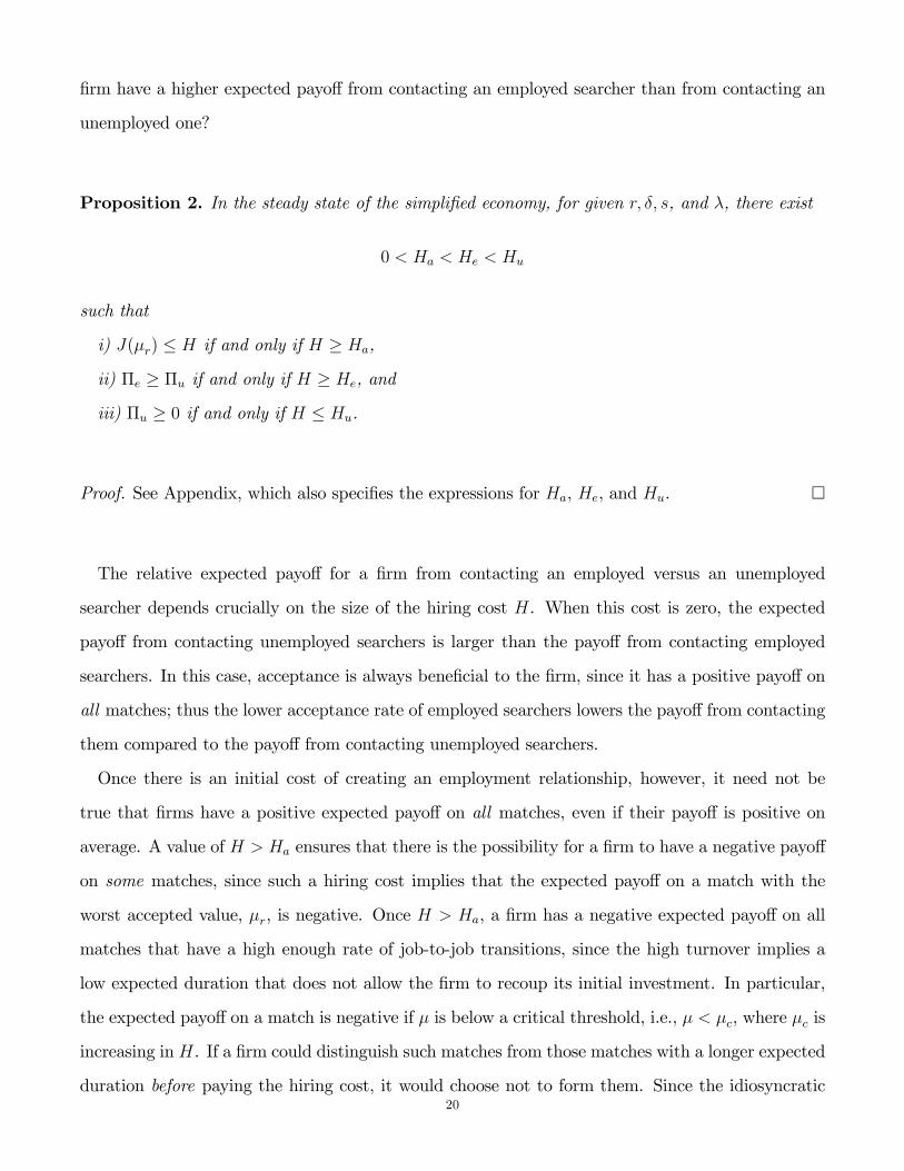
Proposition 2. In the steady state of the simpli�ed economy, for given r; �; s, and �, there exist

0 < Ha < He < Hu

such that

i) J(�r) � H if and only if H � Ha,

ii) �e � �u if and only if H � He, and

iii) �u � 0 if and only if H � Hu.

Proof. See Appendix, which also speci�es the expressions for Ha, He, and Hu. �

The relative expected payo¤ for a �rm from contacting an employed versus an unemployed

searcher depends crucially on the size of the hiring cost H. When this cost is zero, the expected

payo¤ from contacting unemployed searchers is larger than the payo¤ from contacting employed

searchers. In this case, acceptance is always bene�cial to the �rm, since it has a positive payo¤ on

all matches; thus the lower acceptance rate of employed searchers lowers the payo¤ from contacting

them compared to the payo¤ from contacting unemployed searchers.

Once there is an initial cost of creating an employment relationship, however, it need not be

true that �rms have a positive expected payo¤ on all matches, even if their payo¤ is positive on

average. A value of H > Ha ensures that there is the possibility for a �rm to have a negative payo¤

on some matches, since such a hiring cost implies that the expected payo¤ on a match with the

worst accepted value, �r, is negative. Once H > Ha, a �rm has a negative expected payo¤ on all

matches that have a high enough rate of job-to-job transitions, since the high turnover implies a

low expected duration that does not allow the �rm to recoup its initial investment. In particular,

the expected payo¤ on a match is negative if � is below a critical threshold, i.e., � < �c, where �c is

increasing in H. If a �rm could distinguish such matches from those matches with a longer expected

duration before paying the hiring cost, it would choose not to form them. Since the idiosyncratic20

job amenity, �, is not observable by the �rm (at least not prior to paying the hiring cost), �rms will

create such matches as long as match creation has a positive payo¤ in expectation.18

The positive selection of workers into idiosyncratic values toward the top of the distribution that

explains Claim 1 also implies that the high-turnover matches that a �rm accrues a loss on when

H > Ha are exactly the matches with a low idiosyncratic component that unemployed searchers

are more likely to accept. This reduces the payo¤ to a �rm from contacting unemployed searchers.

Proposition 2 states that, for a high enough hiring cost (i.e., for H � He), this e¤ect is so large

that �rms have a lower expected payo¤ from contacting unemployed searchers.

To demonstrate further how a higher payo¤ from contacting employed searchers can arise for a

large enough hiring cost, I plot in Figure 1 the payo¤ to a �rm from creating matches of di¤erent

idiosyncratic components and the probability that these di¤erent matches are accepted by unem-

ployed and employed searchers. (For these calculations, I use the same parameter values that I used

in the quantitative exercises in Section 3 and set s = 0:4.) The �gure shows that it is precisely

the matches that generate negative payo¤s to the �rm that employed searchers are likely to reject,

while unemployed searchers accept jobs indiscriminately.

Proposition 2 de�nes a �nal threshold, Hu, above He. Once the hiring cost is above Hu, the

expected payo¤ from contacting an unemployed worker becomes negative. At values of H above

this threshold, an equilibrium exists only if it is assumed that �rms cannot observe the current

employment status of workers upon meeting them. Otherwise, they would reject hiring the un-

employed workers, which could not be an equilibrium for a positive job-�nding rate. Below this

threshold, the assumption on the observability of the employment status of workers is irrelevant,

since �rms have a positive payo¤ from contacting both employed and unemployed workers. In all

of my quantitative exercises, I set H below Hu.19

18The optimal allocation in this environment would demand that the hiring cost be paid by the worker, the informedparty, and not the �rm. Given that it is the �rm that controls the hiring technology (provides job-speci�c training,for example), implementing the optimal allocation in a decentralized equilibrium would require the �rm to commit toa contract in which the worker transfers to the �rm upfront the hiring and recruiting costs and receives her marginalproduct thereafter. Such a contract is not viable if 1) workers do not have access to su¢ cient amount of borrowing, 2)the �rm cannot commit to future wages so that competing �rms could attract away applicants by o¤ering contractswithout an up-front payment, or 3) if there is an incentive for the �rm to form potentially unproductive relationshipssimply to collect the transfer from the worker without actually expending the cost of appropriately training theworker.

19Propositions 1 and 2 hold in the general model studied in Section 2. It is only the algebra that becomes moretedious.

21

Finally, note that the results in Proposition 2 are for a �xed value of the job-�nding rate �.

The results here should, therefore, be interpreted as a comparison of two economies with di¤erent

hiring costs, but with the same extent of on-the-job search, discount rate, job-destruction rate, and

job-�nding rate.

Next, I study the response of the above economy to changes in aggregate driving forces. Through-

out, I consider the steady state of the simpli�ed model and rely on comparisons of steady states to

assess the response of the model to changes in its parameters.

Proposition 3. Across steady states in the simpli�ed model, the elasticity of the job-�nding rate

with respect to labor productivity is

"�p =p

p� bg��r; �; �; s;H; �

�;

where "xy = d lnxd ln y

and H = Hp�w , here and in the rest of the paper.

In addition, the elasticities of the unemployment rate, the vacancy rate, and the quit rate with

respect to labor productivity are, respectively,

"up = gu (�; �) "�p

"vp ="�p�+ gv (�; �; s) "�p

"qp = gq (�; �; s) "�p:

Given the assumptions about the model parameters, "�p > 0, "up < 0, "vp > 0, and "qp > 0.

Proof. See Appendix, which also speci�es the functional form for g�, gu, gv, and gq. �

The elasticity of the job-�nding rate with respect to labor productivity, "�p, can be expressed

as the product of the elasticity of the �rm�s �ow pro�t margin with respect to labor productivity,

which, given the wage in Equation 1, is pp�b , and a second term g�

�r; �; �; s;H; �

�, which captures

the impact of on-the-job search and of the hiring cost. The same decomposition can be done for

the elasticity of the unemployment rate, of the vacancy rate, and of the quit rate. This means that

the impact of labor productivity shocks on the relevant labor-market variables can be decomposed

into an e¤ect coming through the wage-setting mechanism and an e¤ect coming through turnover.22

This decomposition is useful given the controversies in the literature about the appropriate way to

model wage-setting in matching models.(For a discussion, see Mortensen and Nagypál (2007b).)

The relationship between the elasticity of the unemployment rate and that of the job-�nding

rate is the same in a model with on-the-job search as it is in one without it; i.e., gu does not

depend on s. This is not the case for vacancies, however. Once on-the-job search is introduced,

market tightness is no longer equal to the ratio of vacancies to unemployment. In particular, the

vacancy-unemployment ratio is the product of market tightness and the ratio of total searchers to

unemployed searchers, which is a procyclical variable. This implies that by de�nition, in a model of

on-the-job search, the vacancy-unemployment ratio is more procyclical than is market tightness. It

also means that the ratio of the elasticity of the vacancy rate to the elasticity of the job-�nding rate

increases with the amount of on-the-job search; i.e., @gv@s> 0. This is an important result, since as

we have seen in Section 3, the presence of on-the-job search makes the largest contribution toward

explaining the volatility of the vacancy rate.

In determining the relationship between movements in the quit rate and the job-�nding rate, there

are two e¤ects to consider. First, the quit rate for a worker with a given idiosyncratic component

increases with the job-�nding rate. Second, across steady states, a higher job-�nding rate results

in a shift of workers toward higher idiosyncratic components, which then results in a decrease in

the quit rate. The proposition implies that the �rst e¤ect always dominates, so that the quit rate

unambiguously increases in response to an increase in productivity.

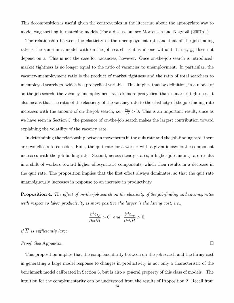
Proposition 4. The e¤ect of on-the-job search on the elasticity of the job-�nding and vacancy rates

with respect to labor productivity is more positive the larger is the hiring cost; i.e.,

@2"�p

@s@H> 0 and

@2"vp

@s@H> 0;

if H is su¢ ciently large.


This proposition implies that the complementarity between on-the-job search and the hiring cost

in generating a large model response to changes in productivity is not only a characteristic of the

benchmark model calibrated in Section 3, but is also a general property of this class of models. The

intuition for the complementarity can be understood from the results of Proposition 2. Recall from23

that proposition that, as H increases, the relative payo¤ from contacting an employed searcher rises.

This result in turn means that the shift in the pool of searchers toward employed workers during an

upturn raises the payo¤ from opening a vacancy, an e¤ect that encourages vacancy creation. Since

the extent of on-the-job search increases in s, this vacancy-creation e¤ect is more pronounced for

higher values of s. To put it di¤erently, given the positive selection of workers into jobs with a

high idiosyncratic component, employees hired from another job have a higher expected duration

over which the cost of hiring can be recouped than do employees hired from unemployment. This

�nding means that the e¤ective cost of hiring is declining in the fraction of new employees hired

from another job, which becomes more procyclical the larger is s.

To demonstrate the extent of this complementarity, Figure 2 plots the elasticity of the job-�nding

rate and the vacancy rate with respect to labor productivity for di¤erent values of s and H; using

the same values for the other parameters as above. The values of H that I consider are from zero to

�ve times the quarterly �ow pro�t of �rms. In panel (a), the value of pp�b

�1�� = 2:30, corresponding

to s = 0 and H = 0, represents the model without any hiring cost or on-the-job search. When

H = 0, the elasticity predicted by the model decreases in s. The decline, though, is relatively mild

for the chosen parameter values, with the elasticity becoming 1:42 when s = 1. It can be shown

that this decline in the elasticity of the job-�nding rate when H = 0 is a general result that holds for

any choice of parameters. The reason for this decline is apparent from Proposition 2: when there

are no hiring costs, it is always more pro�table to contact an unemployed worker so the presence

of employed searchers dampens the variation in the incentives to create vacancies.20 Notice from

panel (b) that this decline is not present for the elasticity of the vacancy rate.

It is clear from Figure 2 that adding a hiring cost to the model without any on-the-job search

increases the elasticity of the job-�nding and vacancy rates with respect to labor productivity, as

we already saw in Section 3. This increase is more pronounced when on-the-job search is present,

especially for vacancies, because of the complementarity discussed in Proposition 4. Given the

assumption that the previous employment status of searchers is observable to �rms upon contact, a

limit can be placed on the amount of ampli�cation predicted by this simpli�ed model. For a large

amount of on-the-job search and a large hiring cost, �rms have a negative expected payo¤ when

contacting an unemployed searcher, since unemployed searchers have low expected duration. The

20This also seems to be the case for the model studied by Pissarides (1994).24

thick line labeled H = Hu in Figure 2 plots the predicted elasticity as a function of s when the

hiring cost is set so that a �rm�s expected payo¤ from contacting an unemployed searcher is exactly

zero, i.e., �u = 0. Below and to the left of this curve lie points where the equilibrium features

�u > 0. Notice that this limit is less binding in the more general model with variable search e¤ort

examined above. There, workers high in the idiosyncratic distribution that provide the highest

payo¤ to �rms choose a low search e¤ort and thus have lower turnover than with a �xed search

e¤ort. In particular, �u > 0 in all the quantitative exercises of Section 3.

Next, I turn examine the response of this simpli�ed economy to changes in the job-destruction

rate.

Proposition 5. Across steady states in the simpli�ed model, the elasticity of the job-�nding rate

with respect to the job-destruction rate is

"�� = h��r; �; �; s;H; �

�:

In addition, the elasticities of the unemployment rate, the vacancy rate, and the quit rate with respect

to the job-destruction rate are, respectively,

"u� = �gu (�; �) (1� "��)

"v� ="�� gv (�; �; s) (1� "��)

"q� = 1� gq (�; �; s) (1� "��) :

Given the assumptions on the model parameters, "�� < 1, "u� > 0, "v� < 1�, and "q� < 1.

Proof. See Appendix, which also speci�es the functional form for h�. �

In contrast with the model without on-the-job search, the elasticity of the job-�nding rate with

respect to the job-destruction rate is not necessarily negative. In the presence of on-the-job search,

one e¤ect of a higher job-destruction rate is to remove workers from jobs at the very top of the idio-

syncratic component distribution and thereby increase the acceptance rate of employed searchers,

encouraging vacancy creation. This e¤ect has the potential to be strong enough to increase the

ratio of vacancies to searchers, thereby increasing the job-�nding rate. The proposition does show,25

however, that this positive e¤ect on the job-�nding rate is never large enough to cause the un-

employment rate to respond negatively to an increase in the job-destruction rate. Below I also

show that for empirically relevant parameter values this positive e¤ect on the job-�nding rate is not

strong enough to cause the elasticity of the job-�nding rate to be positive.

The elasticity of vacancies is the sum of two terms. The �rst term is simply a multiple of the

elasticity of the job-�nding rate; thus, it has the same sign, which is generally negative. The

second term is always positive and decreases in s for a given "��. When s = 0, the second term

is equal to (1 � u) (1� "��). For an "�� that is negative, but close to zero as in the standard

model with empirically relevant parameter values, the second term is much larger than the �rst,

so "v� � 1 � u > 0. In other words, the vacancy rate co-moves positively with the job-destruction

rate and hence also with the unemployment rate, which is greatly at odds with the data, as pointed

out by Shimer (2005). The reason for this result in the standard model is that an increase in the

job-destruction rate increases the number of searching workers, thus encouraging vacancies to enter

the market, even as the vacancy-unemployment ratio declines. Once on-the-job search is added

to the model, however, the impact of an increase in the job-destruction rate on the number of

searchers does decrease, and the weight on the second term declines. When s = 1, a change in

the job-destruction rate has no impact on the number of searchers in the economy, and the second

term in the expression for "v� vanishes; this implies that the elasticity of the vacancy rate has the

same sign as the elasticity of the job-�nding rate, which is generally negative. Adding on-the-job

search thus brings back changes in the job-destruction rate as a source of labor-market �uctuations

in matching models.

The elasticity of the quit rate with respect to the job-destruction rate is not necessarily negative

for the same reasons that the elasticity of the job-�nding rate is not necessarily negative: a higher

job-destruction rate moves workers toward lower idiosyncratic values in the distribution, which

then increases the acceptance rate and, therefore, the quit rate of workers. Unlike in the case of

the job-�nding rate, this e¤ect can be strong enough to cause the elasticity of the quit rate to be

positive, even for empirically relevant parameter values. This explains the small and occasionally

countercyclical response of the quit rate in Section 3 across steady states.

26

Proposition 6. The e¤ect of on-the-job search on the elasticity of the job-�nding and vacancy rates

with respect to the job-destruction rate is more negative the larger the hiring cost, i.e.,

@2"��

@s@H=@2h�

�r; �; �; s;H; �

�@s@H

< 0 and@2"v�

@s@H< 0;

if H is su¢ ciently large and r is su¢ ciently small.


For a large enough hiring cost, there is again a complementarity between on-the-job search and

the hiring cost, where the reason for this complementarity is the same as in the case of labor

productivity. To demonstrate the extent of this complementarity, in Figure 3, I plot the elasticity

with respect to the job-destruction rate of the job-�nding rate and that of the vacancy rate for

di¤erent values of s and H. I again use the same values for the other parameters as in Section 3.

For these values, the model predicts an empirically correct sign for the elasticity of the job-�nding

rate. The model without on-the-job search or a hiring cost (s = 0 and H = 0) corresponds to

a moderate elasticity of the job-�nding rate and an elasticity of the vacancy rate that is close to

0. The elasticity of the job-�nding rate declines in absolute value in s when H = 0, which again

can be shown to be a general property of the simpli�ed model. This decline is very signi�cant,

as the elasticity is �0:60 when s = 0 and is �0:01 when s = 1. Once again, it is clear from

Figure 3 that adding a hiring cost to the model increases the magnitude of the elasticity of the

job-�nding rate with respect to the job-destruction rate, for the same reasons as in the case of

labor productivity. The adding of a hiring cost also increases the absolute value of the elasticity

of the vacancy rate somewhat. Further, Figure 3 clearly demonstrates that the complementarity

discussed in Proposition 6 is again quantitatively relevant. For a hiring cost above two quarters�

of pro�ts, the elasticity of the job-�nding rate increases with s over most of its range, although a

hiring cost of three to four quarters�of pro�ts is again required to generate a quantitatively large

increase in the elasticity with s. Once more, there is a limit to how much ampli�cation can be

generated by the complementarity between the hiring cost and on-the-job search. The thick line

labeled H = Hu in Figure 3 plots the predicted elasticity as a function of s when the hiring cost

is set to make a �rm�s expected payo¤ from contacting an unemployed worker exactly zero, i.e.,

�u = 0. Above and to the left of this curve lie points where the equilibrium features �u > 0.27

5. Empirical evidence

5.1. Job switching and previous employment status. A key component of the proposed model

is that newly employed workers who have been previously unemployed have a higher chance of

switching jobs than newly employed workers who have been previously employed. To show that

this is indeed the case, I consider a sample of individuals ages 25-60 from the Current Population

Surveys from 1994 to 2004, who were observed for two consecutive months and who where hired

into a new job in the �rst month and continue to be employed in the second month, though not

necessarily by the same employer. (For a detailed description of the data construction, see Nagypál

(2005b).) I estimate a logit speci�cation for the probability of switching employers between the two

months controlling for a worker�s sex, race, age, education, and marital status, their job�s industry

and full-time status, and month and year e¤fects. I �nd that previously unemployed workers have a

16:2% higher chance of switching employers than do previously employed workers (with a standard

error of 3:2%). Once I restrict the sample to workers who self-report their own labor-market status,

the e¤ect becomes 19:5% (with a standard error of 5:1%).21 Due to the short panel component of

the Current Population Survey, it is not possible to estimate job-switching probabilities at higher

tenures, but these results certainly suggest that the expected time on a job before switching to

another job is lower for previously unemployed workers.

5.2. Job-destruction shocks. In this paper, I argue that taking into account job-destruction

shocks is important when accounting for the business-cycle volatility of key labor-market variables.

Indeed, in the benchmark model, a signi�cant fraction of the overall response is due to changes in

the job-destruction rate: shutting down the volatility in the job-destruction rate would decrease the

model-implied volatility of the job-�nding rate by 24%, of the unemployment rate by 48%, and of

the vacancy rate by 22%.

The theoretical possibility that, in the presence of on-the-job search, variation in the job-destruction

rate need not induce a positive correlation between the unemployment and vacancy rates has been

discussed above. This brings back job-destruction shocks as a potential driving force into matching

models. To assess how relevant job-destruction shocks are as an actual driving force, notice that

21I have 104,689 observations over the ten years, with 41,592 self-reports.28

these shocks impact the model-implied volatilities through two channels. First, volatility in the sep-

aration rate has a direct impact on the volatility of the unemployment rate. To the extent that a

third of the variation in the unemployment rate is due to variation in the job-destruction/separation

rate margin, taking this volatility into account is necessary to account fully for the variation in

unemployment (and explains why the volatility of the unemployment rate declines the most when

job-destruction shocks are shut down). Second, volatility in the separation rate a¤ects the incentives

to create vacancies in the model by changing the expected duration of newly created employment

matches. Does a higher separation rate indeed signal a lower expected duration of new matches in

the data? There is evidence that indeed it does: Bowlus (1995) and Davis, Haltiwanger, and Schuh

(1996) both o¤er evidence that jobs created during recessions are more likely to be destroyed than

jobs created during booms. Of course, to the extent that the volatility of the separation rate is

partly explained by a burst of job destruction at the beginning of downturns (as argued by Davis,

Haltiwanger, and Schuh (1996) and more recently by Fujita and Ramey (2007a)) which does not

re�ect changes in the expected duration of new matches, the calculations in Table 2 taking into

account all the variation in the job-destruction rate could be somewhat overestimating the varia-

tion in the incentives to create vacancies and the resulting volatility of the job-�nding and vacancy

rates.22

6. Relationship to existing literature

The model I construct builds on the matching framework developed by Diamond (1982), Mortensen

(1982), and Pissarides (1985) (see Pissarides (2000) for a review). In the last two decades, matching

models have gained wide popularity in the analysis of aggregate labor markets due to their abil-

ity to explain several labor-market phenomena that the neoclassical growth model cannot tackle,

such as the existence of equilibrium unemployment. Since the development of the model, several

22Matching models with endogenous destruction are designed to explain the initial burst of job destruction that takesplace in a recession as opposed to the drop in the expected duration of newly created matches. These models donot generate substantially more volatility than the textbook model with exogenous separations (see Mortensen andNagypál (2007a)). Taking endogenous job-destruction into account in the presence of on-the-job search, a naturalframework for which is the model of Nagypál (2005a), could nonetheless be important given the potential promisesuch an extension has for better explaining the cyclical behavior of the quit rate.

29

authors have asserted that it can quantitatively explain the variation in key labor-market vari-

ables over the business cycle.23 Recently, however, this view has been challenged, and the standard

matching model has been criticized for its lack of ampli�cation when compared with data. Shimer

(2005) shows that in response to shocks to the productivity of employment relationships and to

the job-destruction rate, the textbook matching model predicts the volatility of the vacancy and

unemployment rates to be an order of magnitude lower than the volatility observed in the data,

assuming reasonable parameter values. The recent and active literature spurred by Shimer�s work,

starting with Hall (2005), has mostly focused on the role of less responsive wages in resolving this

�recruitment volatility puzzle�.24 While there have been partial successes in bringing the model

in line with the data (see Mortensen and Nagypál (2007b), in particular, who also give a detailed

review of the literature), there has remained a substantial gap between what the model can explain

and what is observed in the data. Recently, Haefke, Sonntag, and van Rens (2007) and Pissarides

(2007) have questioned whether there is enough stickiness empirically in the relevant measure of

wages to explain the observed volatility. All the recent papers addressing the �recruitment volatil-

ity puzzle�have abstracted from on-the-job search, with the exception of Krause and Lubik (2006)

discussed below.

While the focus on the �recruitment volatility puzzle�and the interaction of on-the-job search

and costly hiring is novel, my paper is not the �rst one to study the cyclical implications of matching

models with on-the-job search. Pissarides (1994) and Mortensen (1994) both generalize a matching

model by incorporating on-the-job search. Pissarides (1994) informally speculates that allowing

for search by the employed reduces the responsiveness of unemployment to productivity shocks.

Without a hiring cost, this is also true in my model. The reasons for such a result in his model

are di¤erent than in mine, however. In particular, he develops a model with two type of jobs: bad

jobs that are only taken by unemployed workers and good jobs that are taken both by unemployed

and employed workers. The costs of creating these two types of jobs are set up so that the relative

number of good jobs rises in response to an increase in aggregate labor productivity. With these

good jobs being harder to get for the unemployed due to competition from employed searchers,

23See, for example, Blanchard and Diamond (1989), Mortensen and Pissarides (1994), Andolfatto (1996), Merz(1995), Cole and Rogerson (1999), and Ramey and Watson (1997).24See Kennan (2007), Menzio (2005b), Hall and Milgrom (2007), Hagedorn and Manovskii (2007), and Gertler andTrigari (2006).

30

his conjecture follows. Given the structure of his model though, the acceptance rate of employed

searchers is always unity, so the channels present in my framework with a disperse distribution of

job values do not arise in his model. In the setup of Mortensen (1994), whose aim is to study the

cyclical properties of job �ows implied by his model, all newly created jobs have the highest payo¤

among all jobs, so again the issue of whether to accept a job or not does not arise.

More recently, Krause and Lubik (2006) study a model with on-the-job search and again two types

of jobs: bad jobs that are easy to get and good jobs that are di¢ cult to get in equilibrium. They

assume that search by workers can be directed toward the two types of jobs, which thus creates two

separate markets. While the job-�nding rate in each market varies over the business cycle no more

than in the textbook matching model, a feature of their model is that unemployed workers apply

for more bad jobs in a boom while they wait to get good jobs in a recession. This feature is present

because the authors make the critical, but questionable, assumption that the search technology

available to employed workers is elastic while that available to unemployed workers is inelastic.

This makes unemployed workers want to take bad jobs more in a boom because the on-the-job

search technology becomes more valuable compared to the value of unemployed search. Given that

the job-�nding rate for bad jobs is higher, this composition e¤ect leads to an increased volatility of

the aggregate job-�nding rate.

The setup of Barlevy (2002) is the most similar to the model studied in this paper, although in his

model it is heterogeneity in productivity that motivates on-the-job search while in my model, it is

heterogeneity in job amenity. He argues that recessions are times when the reallocation of employed

workers toward their most productive use is hindered by what he calls the �sullying e¤ect�. To the

extent that the distribution of job amenities shifts downwards in a recession, such a sullying e¤ect

is present in my model as well. The results of this paper are novel, since unlike Barlevy (2002), I

focus on the amount of ampli�cation generated by the model, derive analytical comparative static

results, and discuss the role of the complementarity between hiring costs and on-the-job search in

generating �uctuations.

7. Conclusion

This paper has shown that allowing for on-the-job search and a positive reinforcement between

recruiting activity and search by employed workers is critical to explain the observed large cyclical31

volatility of labor-market aggregates. When workers are searching on the job, �rms that contem-

plate advertising a vacant position need to consider both the probability that a contact with a

searching worker results in an employment relationship and the likelihood that a recruited worker

will quit in the future. In the presence of a moderate hiring cost, �rms expect higher pro�ts from

contacting workers who are less likely to quit, even if these workers have a lower probability of

accepting a job. Employed searchers are exactly such workers: they are less likely to accept a job

o¤ered to them, but if they do accept, they are less likely to quit due to the positive selection of

employed workers into better and better employment matches.

When the payo¤ from contacting employed searchers is higher, the presence of more vacancies

and more employed searchers enhance each other in a boom. This creates more ampli�cation in

a model that takes into account on-the-job search compared to one that abstracts from it. In

addition, in the presence of on-the-job search, changes in the job-destruction rate do not induce a

counterfactual positive correlation between the unemployment and vacancy rates, thereby bringing

back changes in the job-destruction rate as a driving force behind labor-market �uctuations.

The mechanism of the model studied here is not the only mechanism capable of generating positive

reinforcement between recruiting activity and on-the-job search in the context of a randommatching

model. Another class of models can give rise to such reinforcement based on the simple idea that

workers are heterogeneous in the payo¤ they generate to �rms (due to di¤erences in productivity or

di¤erences in turnover rates). If there is a positive correlation between the probability of employment

and the payo¤ a worker generates to an employer, this could also give rise to a higher payo¤ from

contacting employed searchers. While intuition would suggest that such a correlation is certainly

present for older and highly educated workers, it is di¢ cult to argue that such a correlation could

explain all the labor-market volatility of less educated and younger workers.

Incorporating on-the-job search and its interaction with recruiting is important not only in the

study of cyclical volatility. The results of this paper suggest that this interaction is also important

in understanding the response of the aggregate labor market to policy interventions, such as the

provision of unemployment insurance. Moreover, the model of this paper o¤ers a novel framework

to use to study the cost of business cycles in the presence of search externalities.

32

8. Appendix

8.1. The wage bargain. I derive the wage outcome by taking the limit of the equivalent discrete-

time bargaining problem. Assume that time is discrete in increments of �. Timing in the period

[t; t+�) is as follows:

(1) workers and �rms arrive to a period either as matched (with a single partner) or unmatched

(2) matched worker-�rm pairs bargain over the wage for the period

(3) workers decide how much to search during the period

(4) production (in relationships that reached an agreement over the wage) and search takes

place during the period

(5) at the end of the period, existing relationship break down with probability ��e��

(6) workers who searched during the period and �rms participate in the matching process

(7) if a worker or a �rm matches with a new partner, they have to decide whether to continue

their existing relationship (or unemployment or vacancy) or end that relationship and form

the new one

The bargaining between the worker and the �rm over the �ow wage prevailing during the period

[t; t + �) takes place as follows. (The wage is constant during the period. As the length of the

period goes to 0, this assumption becomes unrestrictive.) If the worker and the �rm agree on a

wage, production takes place, and the worker enjoys utility w+� and devotes sw e¤ort to searching

for a better job during the period. If the worker and the �rm fail to agree on a wage today, the

worker enjoys utility b + � and devotes sd e¤ort to searching for a better job during the period,

while the �rm has a payo¤ of 0 during the period. In case of disagreement, the worker and �rm

can resume negotiations at the beginning of the next period. If a worker searches during period

[t; t+�) with e¤ort s, it contacts a new job opportunity during the matching phase with probability

s�t+��e�s�t+�� from the distribution Ft+� (W 0).

The payo¤ of the worker in case of agreement on �ow wage wt is

Wt = maxsw

�(wt + �� k (sw))� + e�r�

�1� ��e��

��sw�t+��e

�sw�t+��Zmax (0;W 0 �Nt+�) dFt+� (W 0) +Nt+�

�+ e�r��e��

�sw�t+��e

�sw�t+��Zmax (0;W 0 � Ut+�) dFt+� (W 0) + Ut+�

��;

33

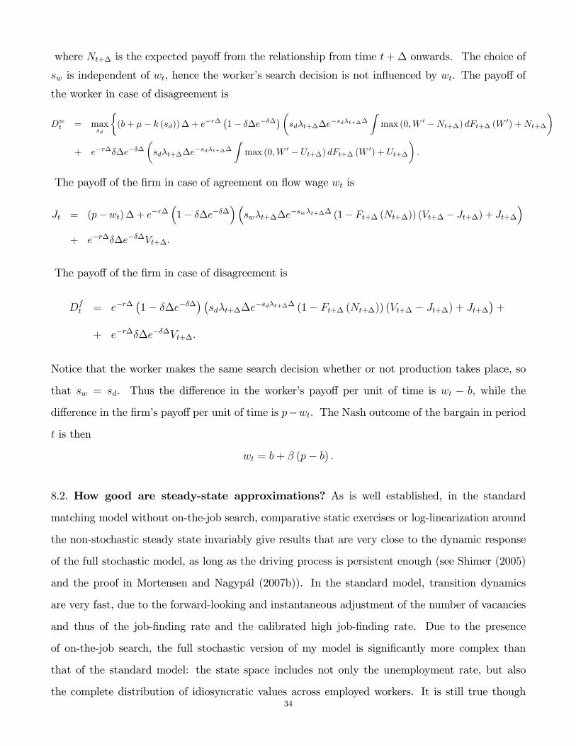
where Nt+� is the expected payo¤ from the relationship from time t+� onwards. The choice of

sw is independent of wt, hence the worker�s search decision is not in�uenced by wt. The payo¤ of

the worker in case of disagreement is

Dwt = max

sd

�(b+ �� k (sd))� + e�r�

�1� ��e��

��sd�t+��e

�sd�t+��Zmax (0;W 0 �Nt+�) dFt+� (W 0) +Nt+�

�+ e�r��e��

�sd�t+��e

�sd�t+��Zmax (0;W 0 � Ut+�) dFt+� (W 0) + Ut+�

�:

The payo¤ of the �rm in case of agreement on �ow wage wt is

Jt = (p� wt)� + e�r��1� ��e��

��sw�t+��e

�sw�t+�� (1� Ft+� (Nt+�)) (Vt+� � Jt+�) + Jt+��

+ e�r��e��Vt+�:

The payo¤ of the �rm in case of disagreement is

Dft = e�r�

�1� ��e��

� �sd�t+��e

�sd�t+�� (1� Ft+� (Nt+�)) (Vt+� � Jt+�) + Jt+��+

+ e�r��e��Vt+�:

Notice that the worker makes the same search decision whether or not production takes place, so

that sw = sd: Thus the di¤erence in the worker�s payo¤ per unit of time is wt � b; while the

di¤erence in the �rm�s payo¤ per unit of time is p�wt: The Nash outcome of the bargain in period

t is then

wt = b+ � (p� b) :

8.2. How good are steady-state approximations? As is well established, in the standard

matching model without on-the-job search, comparative static exercises or log-linearization around

the non-stochastic steady state invariably give results that are very close to the dynamic response

of the full stochastic model, as long as the driving process is persistent enough (see Shimer (2005)

and the proof in Mortensen and Nagypál (2007b)). In the standard model, transition dynamics

are very fast, due to the forward-looking and instantaneous adjustment of the number of vacancies

and thus of the job-�nding rate and the calibrated high job-�nding rate. Due to the presence

of on-the-job search, the full stochastic version of my model is signi�cantly more complex than

that of the standard model: the state space includes not only the unemployment rate, but also

the complete distribution of idiosyncratic values across employed workers. It is still true though34

that there is no delay in the adjustment of vacancies due to the assumption of free entry. Hence,

the dynamics of the dynamic stochastic model along the transition path are determined by the

dynamics of the incentives to create vacancies. These, in turn, are determined by the dynamics of

the two state variables. Since the unemployment rate adjusts just as quickly as in the standard

model due to the high calibrated job-�nding rate, along most of the transition path, the dynamics

of vacancies is determined by the evolution of the distribution of employed workers. For this reason,

given a persistent driving process, the calculated responses of Table 2 in the short run � when the

distribution of employed workers is left unchanged � and in the long run � when the distribution

of employed workers fully adjusts to its new steady-state value � give two useful bounds on the

response of the full dynamic model.

A further important determinant of the similarity of the steady-state approximations to the

full dynamic responses is the persistence of the driving process. Shimer (2005) reports the labor

productivity process to be highly persistent, with a quarterly auto-correlation of 0:878. This means

that using steady-state approximations gives almost identical results to his simulation of the full

stochastic model (an implied volatility of market tightness of 0:034 and 0:035, respectively). Since

the quarterly autocorrelation of the separation rate is somewhat smaller, 0:733, in this case using

steady-state approximations gives slightly larger responses than his simulation of the full stochastic

model (an implied volatility of market tightness of 0:007 and 0:006, respectively). This implies that

my calculations, using steady-state responses, are likely to only slightly overstate the response of

the full stochastic model.

8.3. Useful mathematical facts. Throughout the proofs, I use the following facts.

Fact 1. ln(1+y)y

< 1 for y > 0 and is decreasing in y.

Fact 2. Let n(y) = y(1+y) ln(1+y)

: n0(y) < 0 when y > 0 and limy!0 n(y) = 1.

Fact 3. Let n̂(a; y) = an(ay). @n̂(a;y)@a

> 0 for y > 0.

Proof. By simple algebra. �

8.4. Proof of Proposition 1. The rate at which previously unemployed workers employed at

tenure � � 0 separate from their job is

Su� = � + �s

Z �

�r

F (�)dQu� (�);

35

where Qu� is the distribution of idiosyncratic values among previously unemployed workers at tenure

� . Se� and Qe� can be similarly de�ned. Then, in order to show that S

e� < S

u� , it is su¢ cient to show

that Qe� strictly �rst-order stochastically dominates Qu� for all � � 0.

Given the acceptance decisions of workers, the above distributions at � = 0 can be expressed as

Qu0(�) =F (�)� F (�r)

F (�r)

Qe0(�) =

R ��r(F (�)� F (�0)) dG(�0)R �

�rF (�0)dG(�0)

:

For �; �0 2 [�r; �), de�ne d(�; �0) =F (�)�F (�0)

F (�0). Given the assumptions on F (�), d(�; �0) is strictly

decreasing in �0 since

@d(�; �0)

@�0=�F 0(�0)F (�0) + F 0(�0) (F (�)� F (�0))

F (�02=�F 0(�0)F (�)

F (�02< 0:

Then, for � > �r,

Qe0(�) =

R ��rd(�; �0)F (�0)dG(�0)R ��rF (�0)dG(�0)

<

R ��rd(�; �r)F (�

0)dG(�0)R ��rF (�0)dG(�0)

� d(�; �r) = Qu0(�);

hence the initial distribution of the employed strictly �rst-order stochastically dominates the initial

distribution of the unemployed.

As for the distributions Qu� and Qe� for � > 0, these can be derived from Qu0 and Q

e0 by applying

the same out-�ow rates to them as a function of �, which is �sF (�). Since these rates do not

depend on whether the worker was previously employed or unemployed, the resulting Qe� strictly

�rst-order stochastically dominates Qu� .

8.5. Proof of Proposition 2. In the simpli�ed model, equating the �ows into and out of the

relevant pools gives

(11) u =�

� + �

and

(12) G(�) =u�F (�)

� + �sF (�):

36

The probability that a match of value � is accepted by an employed searcher can be then expressed

as

Ae(�) =G(�)

G(�)=

�F (�)

� + �sF (�);

so that the payo¤ from contacting an employed worker can be written as

�e =

Z �

�

�p� w

r + � + �sF (�)�H

��F (�)

� + �sF (�)dF (�) =

=

Z 1

0

�p� w

r + � + �s(1� x) �H�

�x

� + �s(1� x)dx =

= (p� w) �Z 1

0

1

r + � + �s(1� x)x

� + �s(1� x)dx�H�Z 1

0

x� xr� + �s(1� x)dx;

where I used a change of variables x = F (�). Then, given the de�nite integralsZ 1

0

x

� + �s(1� x)dx =1

�s

�� + �s

�sm1 (�; �; s)� 1

�and Z 1

0

1

r + � + �s(1� x)x

� + �s(1� x)dx =

=1

�2s2r[(� + �s)m1 (�; �; s)� (r + � + �s)m2 (r; �; �; s)] ;

where

m1 (�; �; s) = ln (� + �s)� ln �(13)

m2 (r; �; �; s) = ln (r + � + �s)� ln (r + �) ;(14)

substituting in and simplifying gives

�e =p� w�

�

�sr

�� + �s

sm1 (�; �; s)

�1� rH

�� r + � + �s

sm2 (r; �; �; s) + r�H

�:

Similarly, notice that the payo¤ from contacting an unemployed worker can be written as

�u =

Z �

�

�p� w

r + � + �sF (�)�H

�dF (�) =

=

Z 1

0

�p� w

r + � + �s(1� x) �H�dx =

p� w�

�m2 (r; �; �; s)

s� �H

�:

37

Statement i) of the proposition follows from simple substitution where

Ha =1

r + � + �̂s:

Statement ii) follows from the fact that, for all H,

(15)@�e

@H� @�u@H

=p� w�

� + �s

s

�1� �

�sm1

�> 0;

given Fact 1 of Section 8.3 applied to y = �s�. Similarly, statement iii) of the proposition follows

from @�u@H

= � (p� w) < 0 for all H. The derivation of the expressions

He (r; �; s; �) =(r + �)m2 (r; �; �; s)� �m1 (�; �; s)

r�s� r�m1 (�; �; s)

and

Hu (r; �; s; �) =m2 (r; �; �; s)

�s

is straightforward, given that �e and �u are linear in H. Finally, Hu > He > 0 follows from the

expressions for �e and �u.

8.6. Proof of Proposition 3. Using the expressions for �e and �u derived above, we can rewrite

the job-creation condition in the simpli�ed model as

(16)c

�=

�

�rs((p� w � rH)m1 � (p� w)m2) ;

where again m1 and m2 are de�ned in Equations 13 and 14.

Given the assumptions on the matching function, notice that �d ln �d ln p

= 1��

d ln�d ln p

. Taking logs of

Equation 16 and di¤erentiating with respect to ln p gives

1� ��

d ln�

d ln p= �d ln�

d ln p+ !

��

� � rHd ln �

d ln p+@ lnm1

@ ln�

d ln�

d ln p

�+

+ (1� !)�d ln �

d ln p+@ lnm2

@ ln�

d ln�

d ln p

�;

where

(17) ! =(p� w � rH)m1

(p� w � rH)m1 �m2

:

38

Substituting for the derivatives of m1 and m2 and collecting terms we get�1

�� !

m1

�s

� + �s� 1� !

m2

�s

r + � + �s

�d ln�

d ln p=

�!

rH

1� rH+ 1

�d ln �

d ln p

so that

g��r; �; �; s;H; �

�=!�r; �; �; s;H

�rH1�rH + 1

l�r; �; �; s;H; �

� ;

where

(18) l�r; �; �; s;H; �

�=1

��!�r; �; �; s;H

�m1 (�; �; s)

�s

� + �s�1� !

�r; �; �; s;H

�m2 (r; �; �; s)

�s

r + � + �s:

g� > 0 follows from the fact that l is strictly positive. To see this, note that we can write

l = l1 + l2!, where

l1 =1

�� n

��s

r + �

�>1� ��

> 0

l2 = n

��s

r + �

�� n

��s

�

�> 0;

where the function n(�) is de�ned in Fact 2 of Section 8.3, and the inequalities follow from the

properties of the function n(�) established there.

To derive "up, simply notice that

gu (�; �) =@ lnu

@ ln�= � �

� + �< 0:

To derive "vp, notice that v = � (u+ s(1� u)), so that

@ ln v

@ ln�=

@ ln �

@ ln�+@ ln (u+ s(1� u))

@ ln�=1

�+@ lnu

@ ln�

(1� s)uu+ s(1� u) =

=1

��

� + �

(1� s)�� + s�

� 1

�� 1 > 0;

thus gv (�; �; s) = � ��+�

(1�s)��+s�

.

To derive "qp, �rst derive the quit rate for a general � as

q =�sR ��F (�)dG(�)

1� u = �s

Z �

�

G (�)

1� udF (�) =(19)

= ��s

Z 1

0

x

� + �s(1� x)dx = ��m1 + �sm1 � �s

�s;

39

where the �rst equality follows from integration by parts and the second equality uses the expressions

for u and G(�) in Equations( 11) and (12) and a change of variables with x = F (�). Then

gq (�; �; s) =@ ln q

@ ln�=

�

�m1 + �sm1 � �s

�(� + �s)

@m1

@�+ sm1 � s

�� 1 =(20)

=�sm1

�m1 + �sm1 � �s� 1 = �s� �m1

(�s+ �)m1 � �s> 0;

where the last inequality follows from the fact that gq is decreasing in m1 and m1 <�s�.

8.7. Proof of Theorem 4. The derivation of the result regarding the cross-partial is algebraically

tedious, so here I only sketch the steps of the proof. The �rst step is to notice that, as a function

of s and H, g� can be written as

g� =g1�(s)

g2�(s)� g3�(s)rH;

where both the numerator and the denominator are positive and g3�(s) > 0. Then, suppressing the

dependence on s,

@2g�

@H@s= r

�g3

0� g

1� + g

3�g10�

�g2� � 2g2

0� g

3�g1� +

�g3

0� g

1� � g3�g1

0�

�g3�rH�

g2� � g3�rH�3

To show that @2g�@H@s

> 0 for a su¢ ciently large H, it is enough to show that g30� g

1� � g3�g1

0� > 0. The

next step is to note that

g30

� g1� � g3�g1

0

� =1

s�

�ln (1 + y1)

y21 + y2

� ln (1 + y2)y1

1 + y1

�+

+y1

s (1 + y1)

�y1

1 + y1� y21 + y2

� 1

1 + y1(ln (1 + y1)� ln (1 + y2))

�;

where y1 = �s�and y2 = �s

r+�. Given Fact 2 of Section 8.3, this is decreasing in �, so it is larger than

the same expression evaluated at � = 1, thus

g30

� g1� � g3�g1

0

� �y1

s (1 + y1)

��y1

1 + y1� y21 + y2

��1� ln (1 + y1)

y1

�+ln (1 + y1) y21 + y2

� ln (1 + y2) y11 + y1

�:

This lower bound is positive, in turn, which follows again from Facts 1 and 2 of Section 8.3.

The statement regarding the cross-partial of "vp follows from the fact that

@2"vp

@s@H=@2"�p

@s@H

�1

��

� + �

(1� s) �� + s�

�+@"�p

@H

��

(� + s�)2:

40

8.8. Proof of Proposition 5. To derive the expression for "��, notice that

d lnm1

d ln �=

@ lnm1

@ ln �+@ lnm1

@ ln�

d ln�

d ln �=

�s

m1 (� + �s)

�d ln�

d ln �� 1�

d lnm2

d ln �=

@ lnm2

@ ln �+@ lnm2

@ ln�

d ln�

d ln �=

�s

m2 (r + � + �s)

�d ln�

d ln ��

r + �

�;

where m1 and m2 are de�ned in Equations 13 and 14. Taking logs of the job-creation condition in

Equation (16) and di¤erentiating the result with respect to ln � gives

1� ��

d ln�

d ln �= 1� d ln�

d ln �+ !

d lnm1

d ln �+ (1� !)d lnm2

d ln �:

Substituting in the values of d lnm1

d ln �and d lnm2

d ln �and collecting terms results in

h��r; �; �; s;H; �

�=l�r; �; �; s;H; �

�� 1��

�� !(r;�;�;s;H)�1

m2(r;�;�;s)rr+�

�sr+�+�s

l�r; �; �; s;H; �

� ;

where ! and l are de�ned in Equations (17) and (18).

While the denominator of h� is always positive as shown in the proof of Proposition 3, the sign

of the numerator cannot be generally determined. In fact, numerical calculations show that the

elasticity is positive for some admissible parameter values. Clearly, however, given the fact that

� 2 (0; 1) and ! > 1, the numerator of h� is smaller than its denominator, so "�� < 1:

To derive "up, recall that, when �̂ = �, the unemployment rate is u = ��+�: Then

d lnu

d ln �=

@ lnu

@ ln�

d ln�

d ln �+@ lnu

@ ln �=� (1� "�;�)� + �

:

This is positive since "�� < 1.

To derive "vp, notice that v = � (u+ s(1� u)) implies that

d ln v

d ln �=

d ln �

d ln �+d ln (u+ s(1� u))

d ln �=1

�

d ln�

d ln �+d lnu

d ln �

(1� s)uu+ s(1� u) =

="��+

�

� + �

(1� s)�� + s�

(1� "��) :

This expression is increasing in "�� since 1�> 1 > �

�+�(1�s)��+s�

. Since "�� < 1, this means that "v� is

always less than 1�.

41

Given the expression for the quit rate and for @ ln q@ ln�

in Equations (19) and (20),

"q� =d ln q

d ln �=

@ ln q

@ ln �+@ ln q

@ ln�

d ln�

d ln �= 1 +

�m1 � �s(�s+ �)m1 � �s

+�s� �m1

(�s+ �)m1 � �sd ln�

d ln �=

= 1� �s� �m1

(�s+ �)m1 � �s(1� "��) :

Given "�� < 1 and �s��m1

(�s+�)m1��s > 0 as shown above, we get that "q� < 1.

8.9. Proof of Theorem 6. Again, the proof is algebraically very tedious, so here I only sketch its

basic steps. The �rst step is to notice that, as a function of s and H, h� can be written as

h� = �h1�(s)� h2�(s)rHh3�(s)� h4�(s)rH

;

where the denominator is positive. Then, suppressing the dependence on s,

@2h�

@H@s= �r

�h4

0� h

1� + h

4�h

10� � h2

0� h

3� + h

2�h

30�

�h3� � 2h3

0� h

4�h

2��

h3� � h4�rH�3 +

+ �rh4

0� (h

4�h

1� � 2h2�h3�)�

�h4�h

10� � h2

0� h

3� � h2�h3

0�

�h4��

h3� � h4�rH�3 rH:

To show that @2h�@H@s

< 0 for a su¢ ciently large H, it is enough to show that the numerator of the

second term is negative. This can be done by showing that this expression is a quadratic function

of � that is increasing in � on the interval [0; 1], thus it is always smaller than its value at � = 1,

which can be written as

h2�1

s

y1 � y2y1

y21 + y2

1

1 + y2

�ln (1 + y1)�

y11 + y1

��

y11 + y1

�2!:

This expression is negative if the last term is negative, which happens if and only if

(1 + y1)2 (y1 � ln (1 + y1)) > y21 (y1 � y2) :

This, in turn, holds if y2 is su¢ ciently close to y1, which is the case if r is su¢ ciently small.

The statement regarding the cross-partial of "v� follows from the fact that

@2"v�

@s@H=@2"��

@s@H

�1

��

� + �

(1� s) �� + s�

�+@"��

@H

��

(� + s�)2:

42

References

Andolfatto, D. (1996): �Business Cycles and Labor-Market Search,�American Economic Review, 86(1), 112�132.

Barlevy, G. (2002): �The Sullying E¤ect of Recessions,�Review of Economic Studies, 69(1), 65�96.

Blanchard, O. J., and P. Diamond (1989): �The Beveridge Curve,�Brookings Papers on Economic Activity, 1,

1�60.

Bowlus, A. J. (1995): �Matching Workers and Jobs: Cyclical Fluctuations in Match Quality,� Journal of Labor

Economics, 13(2), 335�350.

Christensen, B. J., R. Lentz, D. Mortensen, G. R. Neumann, and A. Werwatz (2005): �On-the-Job

Search and the Wage Distribution,�Journal of Labor Economics, 23(1), 31�58.

Cole, H., and R. Rogerson (1999): �Can the Mortensen-Pissarides Matching Model Match the Business Cycle

Facts?,�International Economic Review, 40(4), 933�959.

Davis, S. J., J. C. Haltiwanger, and S. Schuh (1996): Job Creation and Job Destruction. The MIT Press,

Cambridge, Massachusetts.

Devine, T. J., and N. M. Kiefer (1991): Empirical Labor Economics: The Search Approach. Oxford University

Press.

Diamond, P. (1982): �Wage Determination and E¢ ciency in Search Equilibrium,�Review of Economic Studies,

49(2), 217�227.

Faberman, R. J. (2005): �Studying the Labor Market with the Job Openings and Labor Turnover Survey,�Bureau

of Labor Statistics working paper No. 388.

Fujita, S., and G. Ramey (2007a): �The Cyclicality of Job Loss and Hiring,�University of California San Diego

mimeo.

(2007b): �Job Matching and Propagation,�Journal of Economic Dynamics and Control, in press.

Gertler, M., and A. Trigari (2006): �Unemployment Fluctuations with Staggered Nash Wage Bargaining,�

New York University mimeo.

Grossman, S., andM. Perry (1986): �Sequential Bargaining with Assymetric Information,�Journal of Economic

Theory, 39, 120�154.

Gul, F., and H. Sonnenschein (1988): �On Delay in Bargaining with One-Sided Uncertainty,�Econometrica,

56(3), 601�611.

Haefke, C., M. Sonntag, and T. van Rens (2007): �Wage Rigidity and Job Creation,�Universitat Pompeu

Fabra mimeo.

Hagedorn, M., and I. Manovskii (2007): �The Cyclical Behavior of Equilibrium Unemployment and Vacancies

Revisited,�University of Pennsylvania mimeo.

Hall, R. E. (2005): �Employment Fluctuations with Equilibrium Wage Stickiness,�American Economic Review,

95(1), 50�65.

43

Hall, R. E., and P. Milgrom (2007): �The Limited In�uence of Unemployment on the Wage Bargain,�Stanford

University mimeo.

Kennan, J. (2007): �Private Information, Wage Bargaining, and Employment Fluctuations,� University of

Wisconsin-Madison mimeo.

Krause, M., and T. Lubik (2006): �On-the-Job Search and the Cylical Dynamics of the Labor Market,�Federal

Reserve of Richmond mimeo.

Menzio, G. (2005a): �A Cheap-Talk Theory of Random and Directed Search,�University of Pennsylvania mimeo.

(2005b): �High Frequency Wage Rigidity,�University of Pennsylvania mimeo.

Merz, M. (1995): �Search in the Labor Market and the Real Business Cycle,� Journal of Monetary Economics,

36(2), 269�300.

Mortensen, D., and E. Nagypál (2007a): �Labor-Market Volatility in Matching Models with Endogenous

Separations,�forthcoming.

(2007b): �More on Unemployment and Vacancy Fluctuations,� Review of Economic Dynamics, 10(3),

327�347.

Mortensen, D. T. (1982): �Property Rights and E¢ ciency in Mating, Racing, and Related Games,�American

Economic Review, 72, 968�979.

(1994): �The Cyclical Behavior of Job and Worker Flows,� Journal of Economic Dynamics and Control,

18(6), 1121�1142.

Mortensen, D. T., and C. A. Pissarides (1994): �Job Creation and Job Destruction in the Theory of Unem-

ployment,�Review of Economic Studies, 61(3), 397�415.

Nagypál, E. (2005a): �On the extent of job-to-job transitions,�Northwestern University mimeo.

(2005b): �Worker Reallocation over the Business Cycle: The Importance of Job-to-Job Transitions,�

Northwestern University mimeo.

Petrongolo, B., and C. Pissarides (2001): �Looking into the Black Box: A Survey of the Matching Function,�

Journal of Economic Literature, 39, 390�431.

Pissarides, C. A. (1985): �Short-Run Equilibrium Dynamics of Unemployment, Vacancies and Real Wages,�

American Economic Review, 75, 968�979.

(1994): �Search Unemployment with On-the-Job Search,�Review of Economic Studies, 61(3), 457�75.

(2000): Equilibrium Unemployment Theory. The MIT Press, 2 edn.

(2007): �The Unemployment Volatility Puzzle: Is Wage Stickiness the Answer?,�Walras Bowley lecture,

North American Summer Meeting of the Econometric Society.

Ramey, G., and J. Watson (1997): �Contractual Fragility, Job Destruction, and Business Cycles,�Quarterly

Journal of Economics, 112(3), 873�911.

Shimer, R. (2005): �The Cyclical Behavior of Equilibrium Unemployment and Vacancies,� American Economic

Review, 95(1), 25�49.44

(2006): �On-the-Job Search and Strategic Bargaining,� in Structural Models of Wage and Employment

Dynamics, Contributions to Economic Analysis. Elsevier Science B.V.

45

Figures

0.1 0.08 0.06 0.04 0.02 0 0.02 0.04 0.06 0.08 0.1

0

1

idiosyncratic component

acce

ptan

cepr

obab

ility

0.1 0.08 0.06 0.04 0.02 0 0.02 0.04 0.06 0.08 0.1

0ex

pect

edpa

yoff

offir

mfr

omco

ntac

t

acceptance probablity of the employed

acceptance probablity of the unemployed

firm payoff

Figure 1. Firms�expected payo¤ from contacting workers with di¤erent idiosyn-cratic components and the probability of acceptance of unemployed and employedsearchers as a function of their idiosyncratic component.

46

0 0.1 0.2 0.3 0.4 0.5 0.6 0.7 0.8 0.9 10

2

4

6

8

10

12

search effort of employed workers, s

elas

ticity

ofjo

bfin

ding

rate

,ε λ

p

H=πH=2π

H=3π

H=4π

H=5π

H=0

H=Hu

0 0.1 0.2 0.3 0.4 0.5 0.6 0.7 0.8 0.9 10

5

10

15

20

25

30


elas

ticity

ofva

canc

yra

te,

ε vp

H=πH=2π

H=3π

H=4π

H=5π

H=0

H=Hu

Figure 2. Elasticity of the job-�nding rate (top panel) and of the vacancy rate(bottom panel) with respect to labor productivity as a function of the search e¤ort ofemployed workers for di¤erent values of the hiring cost, H (expressed as a multipleof �ow pro�ts per quarter, �).

47

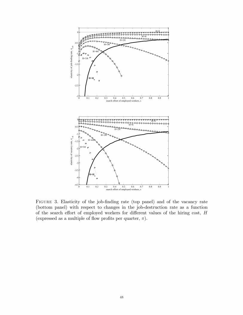
0 0.1 0.2 0.3 0.4 0.5 0.6 0.7 0.8 0.9 13

2.5

2

1.5

1

0.5

0


elas

ticity

ofjo

bfin

ding

rate

,ε λ

δ

H=π

H=2π

H=3π

H=4π

H=5π

H=0

H=Hu

0 0.1 0.2 0.3 0.4 0.5 0.6 0.7 0.8 0.9 14.5

4

3.5

3

2.5

2

1.5

1

0.5

0


elas

ticity

ofva

canc

yra

te,

ε vδ

H=π

H=2π

H=3π

H=4π

H=5π

H=0

H=Hu

Figure 3. Elasticity of the job-�nding rate (top panel) and of the vacancy rate(bottom panel) with respect to changes in the job-destruction rate as a functionof the search e¤ort of employed workers for di¤erent values of the hiring cost, H(expressed as a multiple of �ow pro�ts per quarter, �).

48

0.1 0.08 0.06 0.04 0.02 0 0.02 0.04 0.06 0.08 0.10

1

match quality

sear

chef

fort

rela

tive

toun

empl

oyed

wor

kers

0.1 0.08 0.06 0.04 0.02 0 0.02 0.04 0.06 0.08 0.10

dens

ityof

dist

ribut

ion

func

tion

search effort

initial match quality distribution

equilibrium match quality distribution

Figure 4. Equilibrium search e¤ort as a function of the idiosyncratic componentand the initial and equilibrium distribution of idiosyncratic component in the modelwith variable search e¤ort.

0 0.5 1 1.5 2 2.5 3 3.50.05

0.1

0.15

0.2

hiring cost (as a multiple of quarterly profits)

mod

elim

plie

dvo

latil

ityof

job

findi

ngra

te

withonthejobsearch

withoutonthejobsearch

49

0 0.5 1 1.5 2 2.5 3 3.50.05

0.1

0.15

0.2

0.25

0.3

hiring cost (as a multiple of quarterly profits)

mod

elim

plie

dvo

latil

ityof

vaca

ncy

rate

withonthejobsearch

withoutonthejobsearch

Figure 5. Model-implied volatility of the job-�nding rate (top panel) and of thevacancy rate (bottom panel) as a function of the hiring cost with and without on-the-job search.

50

labor-market fluctuations and on-the-job...

Documents