An Investigation of Co-worker and Consumer Discrimination:

The Case of Major League Baseball

Zachary H. Sugarman

Faculty Advisor: Professor Frank Westhoff

Submitted to the Department of Economics of Amherst College in partial fulfillment of the requirements for the degree of Bachelor of Arts with

Distinction

April 22, 2005

Acknowledgments

First, I would like to thank my faculty advisor, Professor Frank Westhoff, for devoting so much time and effort into helping me complete this endeavor. Our humorous daily exchanges kept me sane throughout this process, and there was never a time in which you were unavailable to lend your guidance. I am eternally grateful for these things. After four years of your tutelage, I will always remember one thing: whenever I am unsure about what to do, I should pause and think of what the Pittsburgh Steelers would do, and then do the opposite. (Long live the San Diego Chargers, 1994 AFC Champions!!)

I would also like to thank Jeanne Reinle, secretary of the Department of Economics of Amherst College, for making my daily date with the dreaded economics lab more enjoyable through her caring and lively personality.

To my parents, I am indebted for the numerous times that you brain-stormed with me and offered your advice. No words can express my appreciation for you two always being there to listen to my struggles, no matter how trivial, and supply your loving support. It is ok that you do not understand the multivariable calculus presented in this paper. As long as you perform your obligatory parental duties of exalting my thesis because I am your son, then I will be just fine.

Finally, I would like to acknowledge anyone and everyone who put up with me throughout this grueling process. Thank you all for being so nice.

2

"Man may penetrate the outer reaches of the universe, he may solve the very secret of eternity itself, but for me, the ultimate human experience is to witness the flawless execution of a hit-and-run." -Branch Rickey

Introduction

When laymen refer to discrimination, they often focus on prejudice and violence toward

specific groups (women, homosexuals, Jews, etc.). Economists generally concern themselves

with discrimination in the labor market, however. Over the last fifty years, economists have

increasingly examined discrimination in the labor market for the case of professional sports. This

paper follows that trend and analyzes the presence of racial discrimination in Major League

Baseball in the second half of the twentieth century. Professional sports leagues are an excellent

market in which to study discrimination because they compile readily available detailed statistics

of player performance that provide a measure of productivity. This is especially true for baseball.

Such data are typically unavailable in other markets; thus, one must use imperfect proxies such as

education, experience, and training as measurements of productivity when investigating

discrimination in these markets.

Microeconomic theory suggests that discrimination is derived from three sources: 1)

employers; 2) co-workers; and 3) consumers. This paper investigates the latter two sources of

discrimination through two individual models. The first model studies co-worker discrimination

by analyzing the relationship between a team’s winning percentage and the relative number of

black and Hispanic players in the starting lineup, controlling for player quality. The second

model investigates consumer discrimination by evaluating the relationship between fan

attendance and the number of black and Hispanic starters, controlling for city characteristics,

team quality, and league-specific characteristics. Both ordinary least squares and fixed effects

models are used to analyze this relationship; in addition, the hypothesis that consumer

discrimination varied from the American League to the National League was tested. Both models

analyze every team for each year of its existence during the interval 1950-1999.

3

The first model assumes that co-worker discrimination could affect “team chemistry” (all non-

performance team interactions that impact the ability to win). This model treats the effects of

consumer discrimination on team chemistry in two ways: through a linear deviation variable and

a deviation squared variable for both black and Hispanic ballplayers. There are two major

conclusions that can be made from these results. 1) In the Early Years, black and Hispanic

starters had a surprising positive effect on winning percentage, even after controlling for their

individual skills. 2) In regard to black starters, there was a “segregation effect” in which teams

with a higher degree of segregation enjoyed greater success from 1950-1999. This result suggests

both white and black co-worker discrimination: whites liked to play with whites and blacks liked

to play with blacks. The magnitude of this effect decreased over time and was absent in terms of

Hispanic starters.

The model used to investigate consumer discrimination indicates that neither black nor

Hispanic starters affected annual attendance after 1970. On the other hand, there is evidence that

minority starters had an effect on attendance in the 1950s and 1960s. The results suggest that

blacks had a positive effect and Hispanics a negative effect. However, I now have some

misgivings about the basic structure of this model upon reflection. I fear it does not capture

several important factors that influence attendance.

This paper is organized as follows. The first chapter provides a summary of microeconomic

labor market theory and presents a brief history of the Major League Baseball labor market. An

explanation of the theory of discrimination and an overview of recent studies analyzing

discrimination in baseball are offered in the second chapter. Methodology is explained and

results are provided and analyzed in the third chapter. The paper concludes with a brief summary

of my findings and suggestions for further research.

4

Chapter 1: Summary of Labor Market Theory and History of MLB Labor Market

In a perfect competitive market, price and quantity are determined by the market demand and

supply curves. The market demand curve for labor is the horizontal sum of each individual firm’s

demand curve for labor while the market supply curve for labor is the horizontal sum of each

individual household’s supply curve for labor.

Labor Demand

An individual firm’s demand for labor derives from the demand for the specific output that the

labor is used to produce. Therefore, workers are hired for the contribution they can make toward

producing some good or service for sale. For the purposes of this study, it is sufficient to

consider the one input case in which the production function is Q = f(L). The production function

exhibits diminishing marginal product of labor, MPL. That is, the MPL, the change in Q resulting

from a one unit change in L, decreases as the quantity of labor increases.

Consequently: df > 0, d 2 f <0; where MPL = df dL dL2 dL

Each firm is assumed to strive to maximize profit. Thus, the firm demands the profit

maximizing quantity of labor. Profit = Total Revenue – Total Cost; π = TR – TC.

The profit maximizing quantity of labor is the quantity when dTR = dTC. (Equation 1.1) dL dL

Looking at the left hand side of equation 1.1: dTR is the marginal revenue product of dL

Wage

Quantity of Labor

MarketSupply

MarketDemand

Competitive Labor Market Figure 1.1

w*

L*

5

labor, MRPL. It represents the change in TR from a one unit change in the quantity of labor hired.

MRPL can be factored into two products: 1) the increase in Q that one more unit of L produces;

and 2) the increase in TR that results from that Q.

This can be expressed mathematically: dTR = dTR x dQ , dL dQ dL

which is equivalent to MRPL = MPL x MR, (Equation 1.2) where marginal revenue (MR) is the

change in total revenue resulting from a one unit change in the quantity of output produced. (The

marginal product of labor (MPL) has been previously defined.) As a consequence of diminishing

marginal product of labor, the MRPL slopes downward.1

Looking at the right-hand side of the equation 1.2: dTC is the marginal expense of labor, dL

MEL, and it equals the change in total cost resulting from a one unit change in the quantity of

labor hired. Since labor is the only input in this analysis; TC =wL and:

MEL = dTC = w + L dw . (Equation 1.3) dL dL

In a perfectly competitive labor market, dw = 0 ; thus, MEL = w. dL

The firm’s profit-maximizing quantity of labor is determined by equating Eq. 1.2 and 1.3. Thus,

to maximize profit in a perfectly competitive labor market, a firm will hire labor up until the point

where MRPL = w.

1 The MRPL curve slopes downward in both perfect and imperfect product markets: The MPL curve slopes downward in both markets. With perfect competition, MR is equal to the price of the output, a constant; therefore, the MR curve is flat. In a market with imperfect competition, such as a monopoly, the MR curve slopes downward. Therefore, the slope of MPL x MR (MRPL) is downward sloping in both markets.

6

The individual firm’s demand curve for labor is its marginal revenue product of labor curve.

Consequently, the demand curve slopes downward.2 It follows that the market demand curve for

labor is also downward sloping because it is simply the horizontal sum of each individual firm’s

demand curve for labor. (See Figure 1.1)

Labor Supply

An individual household’s supply curve for labor is based on utility maximization. When

deciding the number of hours to work, the household faces a tradeoff between consumption of

goods (through its earnings) and leisure. This tradeoff can be depicted by a household’s utility

function that includes consumption goods and leisure:

Utility = U(F,C); F = leisure, C = consumption goods. The decision about the number hours

of labor to supply is given by the solution to the household’s constrained utility

maximization problem: max U(F, C) s.t. wF +C = 24w.3

Microeconomic theory shows that the solution to this problem is the point where the marginal

rate of substitution between F and C is equal to the wage: MRS = w.

2 While geometrically the same, these two curves provide very different information. The MRPL expresses a firm’s marginal revenue product in terms of the amount of labor it uses; whereas, a firm’s demand curve expresses the quantity of labor the firm demands in terms of the wage. 3 L + F = 24 and C = earnings = wL; substitution of these equations yields the constraint.

Wage

Quantity of Labor

MRPL

w

LFigure 1.2

MEL = w

7

This study assumes that an increase in wage decreases a household’s preference for leisure.

Therefore, it is assumed that the household’s supply curve for labor is upward sloping.4 As a

result, the market supply curve for labor is also upward sloping. (See Figure 1.1)

The Case of Monopsony

Next consider the polar opposite case of a perfectly competitive labor market: monopsony. A

monopsony labor market is one in which there is a single demander and many suppliers of labor.

Monopsony is the buying-side equivalent of a selling-side monopoly. Like a monopoly seller, a

monopsony buyer is a price maker.

Thus for a monopsony, dw > 0 where for a competitive market dw = 0. dL dL

Recall that MRPL = w + L dw. dL

In a monopsony MRPL = w + (positive value); while in a competitive market MRPL = w.

That is, MRPL > w in a monopsony. As a result, the quantity of labor is equal to Lm < L*

and the wage is wm < w* in a monopsony market.

4 This implies that the substitution effect dominates the income effect in the household’s decision to work.

C

F24

24wU(F,C)

C*

F*

Solution

Figure 1.3

8

A monopsony results in a lower wage and lower level of employment. Unlike the perfectly

competitive case, the wage falls short of MRPL.

Baseball Labor Market: A Brief History

This section will describe the market for players in Major League Baseball and address the

question – Is MLB a monopsony? It will be demonstrated that while MLB still exhibits some

monopsonistic tendencies, there has been a considerable decrease in its monopsony power from

the Reserve Clause Era to the Free Agency Era.

Reserve Clause Era

All baseball players were bound by the “reserve” clause prior to the establishment of free

agency in 1976. Created in 1879, the reserve clause essentially stated that a player could be

‘reserved’ by the owner to play for the same salary as the previous season if he and the owner

could not reach an agreement on the player’s salary for the upcoming season. In this manner, all

rights to a player’s contract belonged to the team; a player could never escape from that club or

seek competing bids from other teams unless his team permitted him to do so. A player could

only negotiate with another team if he was released from the team that contracted him;

furthermore, the team that contracted him had the right to trade the player at its whim.5 Basically,

5 Players were not even able to invalidate a contract by sitting out for a year and then returning to the game.

Wage

Quantity of Labor

Figure 1.4

MRPL

S

MEL

wm

w*

Lm L*

B

C

A

9

the club could buy, sell, or trade a player via his contract as if he was the club’s property. Simon

Rottenberg summarized the reserve rule in his seminal work when he wrote: “the reserve rule,

which binds a player to the team that contracts him, gives a prima facie appearance of monopsony

to the market. Once having signed a first contract, a player is confronted by a single buyer who

may unilaterally specify the price to be paid for his services.” (1956) Therefore, in each

individual team’s market for players, the team operated as the sole buyer of player inputs. Thus,

there is no doubt that the market for players was a monopsony market during this time period.

The reign of the reserve clause lasted a century during which it withstood several challenges in

court. For example, the reserve clause was challenged in court as monopolistic and in violation

of the Sherman Anti-Trust Act in 1922. The Supreme Court unanimously ruled against the case

and gave baseball its infamous ‘anti-trust’ exemption when Chief Justice Wendall declared that

MLB failed to meet the definition of interstate commerce. Fifty years later, the reserve clause

was challenged again, this time by Curt Flood, a star player for the St Louis Cardinals. Flood had

been traded to the Philadelphia Phillies in 1970 but refused to leave the Cardinals, demanding to

play out his contract in St Louis. MLB insisted that Flood either play for the Phillies or retire.

Flood, in turn, sued MLB for violation of antitrust laws. The case reached the Supreme Court in

1972 and, again, the court sided with MLB, citing its anti-trust exemption. This time, however,

the Court said that the anti-trust rule should be overturned, but argued that it was Congress’s

responsibility to do so.

Even though Flood lost his case, the controversy he generated sparked intense debate over the

legality/legitimacy of the reserve clause. This debate escalated in 1975 when Andy Messersmith

and Dave McNally played the entire 1975 season without signing a contract. Messersmith and

McNally filed a joint grievance against baseball's reserve clause after the season, challenging the

clause because it allowed teams to perpetually sign players for 1-year contracts.  Filing a

grievance led their case to be heard by an arbitrator instead of a court. And in December of 1975,

Arbitrator Peter Seitz ruled in favor of Messermsith and McNally. Seitz concluded that the

10

reserve clause granted a team only one additional year of service from a player, thereby ending

the perpetual renewal rights clubs had claimed for so long. Shortly afterward, at the All-Star

break in 1976, the players signed a new Basic Agreement that granted any player with four years

of Major League experience the right to become a free agent after his contract expired. The reign

of the reserve clause was over; players could now seek employment and enter into a contract with

another team when their employment contract with a particular team expired.

Free Agency Era

All players, after four years in MLB, could be free agents if their current contract had expired

or if they could not agree upon a new contract.6 With the advent of free agency, players were no

longer perpetually tied to a single team; they could now bargain with any and all teams. As a

result, average player salaries increased dramatically. The average salary increased from $45,000

in 1975 to $144,000 in 1980. The average salary continued to rise: $372,000 in 1985,

$1,071,029 in 1995, and about $2,000,000 today.

This increase in average salary is consistent with the microeconomic theory explained earlier

in the chapter. Recall that w < MRPL in a monopsony market. Elimination of the reserve clause

and the advent of free agency decreased a MLB team’s capacity for monopsonistic exploitation

and shifted the player market toward a more competitive market. Therefore, the observed

increase in the average player salary is consistent with microeconomic theory, which suggests

that the wage should increase as more competition forces teams to pay players closer to their

MRPL. That is, teams bidding for a player’s services results in the convergence of salary/wage

and MRPL7.

Although free agency has definitely increased the competitive nature of the MLB labor

market, there are still characteristics of the market that allow for some monopsonistic

exploitation. First, there is a long-standing agreement between MLB owners and the player’s

6 The year requirement is not applicable if the club does not offer a contract renewal.7 A baseball player’s MRPL is generally calculated by the determining the revenue generated from the increase in wins from the player’s performance. More complex calculations include the revenue generated from player merchandise, advertising, etc.

11

union that amateur players must be drafted by individual clubs and must sign with the club that

drafts them or sit, out one year. Therefore, the amateur player draft creates a situation in which a

monopsony exists.8 These rookie contracts are valid for seven years and cannot be re-negotiated

until the player has fulfilled at least three years of the contract. Second, MLB has strict barriers

to entry. The owners of MLB franchises have created strict rules over the number of teams in the

industry (30) and the number of players that can be hired by each team (the active roster is

limited to 25 players, except for spring-training when clubs can have 40 players). No new club

can be added to MLB, no new firm can enter the market, without consensus from all of the

owners.

Third, it is important to note that several related firms may collude in hiring decisions and

establish some sort of monopsonistic power over a particular market, in this case the labor

market. If all firms in a given industry agree not to pay employees above a certain wage, they are

no longer in direct competition for labor; the firms act, in essence, as a single firm. (Workers are

forced either to sell their input at the agreed upon rate or to move to another industry). From

1986-1987, the MLB players union filed three grievances against the owners, claiming they were

colluding by refusing to hire free agents from another team. Arbitrators ruled in favor of the

players in all three grievances; the owners were forced to pay the players union over $100

million. The players union hinted at filing another collusion grievance in 2003 but refrained. It

appears obvious that even though the MLB player market is more competitive under free agency

than under the reserve clause, monopsonistic activities continue to occur.

Several studies concluded that some degree of monopsonistic exploitation still exists in MLB.

Gill and Brajer (1992) estimated the level of monopsony exploitation for non-free agents to be

between .295 and .574. That is, these players are paid between 42% and 70% of what they might

be worth in a competitive market. Zimbalist (1992) and Kahn (1991) also conclude that players

8 The amateur player draft is for college and high-school baseball players; it does not include foreigners who play professionally abroad. These players enter the market as free-agents and can negotiate a contract with any club.

12

are paid less than their MRPL. Thus, there is remains clear evidence of monopsony underpayment

in the MLB player market. However, the degree of monopsonistic exploitation has diminished

severely since the inception of free agency.

Chapter 2: Economic Theory of Discrimination and Background Literature

The word discrimination usually conjures up images of prejudice and violence toward a

specific minority group, women, homosexuals, Jews, etc. Economists generally concern

themselves with discrimination in the labor market, however. Kenneth Arrow defines

discrimination as the concept that personal characteristics of the worker that are unrelated to

productivity (male/female, black/white, American/foreign etc.) are also valued on the market.

(1972) This section will demonstrate that discrimination in the labor market manifests in a

decrease of the individual firm’s and, thus, the market demand for labor of the discriminated

against group. The discriminated group will consequently have less employment and lower

wages relative to the non-discriminated group.

A growing number of studies have examined racial discrimination in sports over the last fifty

years. Many economists see professional sports as a good ‘laboratory’ in which to test the theory

of discrimination because professional sports leagues compile detailed statistics of player

performance that provide a measure of productivity. Such data are typically unavailable in most

other industries; this forces the use of proxies such as education, experience, and training for

measurements of productivity. These proxies are imperfect and not as reliable as hard data on

performance. Therefore, the readily available performance data give sports markets an advantage

in testing the economic theory of discrimination. Realizing these advantages, this paper will

study discrimination in Major League Baseball.9

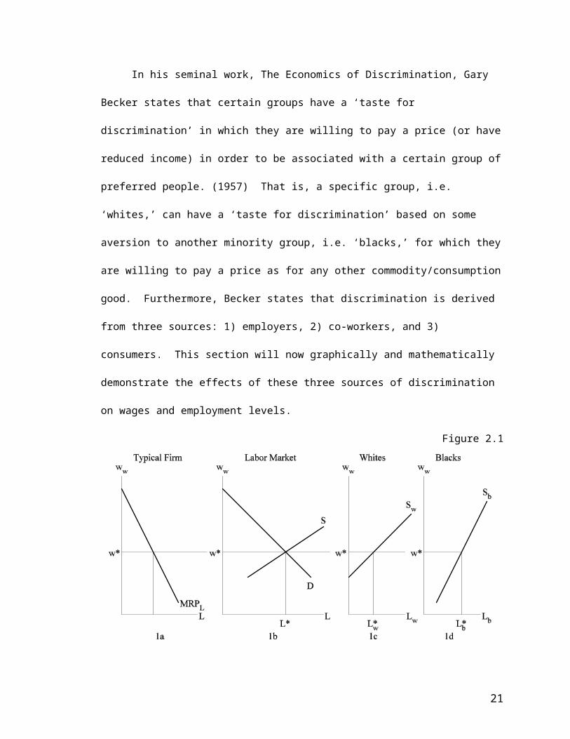
In his seminal work, The Economics of Discrimination, Gary Becker states that certain groups

have a ‘taste for discrimination’ in which they are willing to pay a price (or have reduced income)

9 Within the realm of professional sports leagues, MLB is arguably the best ‘laboratory’ in which to study discrimination because it provides the largest number of statistics that are representative of individual productivity.

13

in order to be associated with a certain group of preferred people. (1957) That is, a specific

group, i.e. ‘whites,’ can have a ‘taste for discrimination’ based on some aversion to another

minority group, i.e. ‘blacks,’ for which they are willing to pay a price as for any other

commodity/consumption good. Furthermore, Becker states that discrimination is derived from

three sources: 1) employers, 2) co-workers, and 3) consumers. This section will now graphically

and mathematically demonstrate the effects of these three sources of discrimination on wages and

employment levels.

Figure 2.1

The graphs above show a competitive labor market with no discrimination in which the labor

force is made up of two types of workers, whites and blacks. For the purpose of this analysis it is

assumed that black and white workers are equally productive. Consequently, the marginal

product of labor equals the sum of white and black workers. Recall that in a competitive market,

a typical firm’s demand for labor curve is the geometric equivalent of workers’ MRPL curve

(1a)10. The market demand curve for labor (1b) is the sum of all individual firms’ demand curves

for labor. The market supply curve for labor (1b) is the horizontal sum of the supply curves for

white (1c) and black workers (1d). A profit-maximizing firm hires labor up to the point where

MRPL = MEL; each firm’s MEL equals the wage in a perfectly competitive labor market; therefore

10 Remember that the demand curve represents the demand of both white and black laborers. Therefore, the slope of the demand curve is twice the slope of the MRPL in 1a.

14

MRPL = w. In competitive market equilibrium, the quantity of labor demanded equals the

quantity of labor supplied. Thus, there will be L* (where L* = Lw* + Lb

*) number of workers each

being paid a wage = w*. (Note that both black workers and white workers are paid the same wage

and that Lw* = Lb*.)

Figure 2.2 Following Becker’s lead I shall consider the three sources of discrimination: 1) employers; 2)

co-workers; and 3) consumers. The effects of discrimination from each of the three sources can

be demonstrated by the same graphical changes seen above.

1) In the case of employer discrimination, an individual employer hires a minority (black)

worker only when the MRPLb exceeds the wage by the discrimination factor de.

That is, MRPLb = wb + de. (Equation 2.1)

Recall that in a competitive labor market, a typical firm hires up to the point in which MRPL = w.

Therefore, the wage paid to the black worker will be de less than the wage paid to the white

worker. The eventual equilibrium condition is that wb = ww – de. When analyzing the market in

terms of white wages (ww), the supply curve for black labor shifts up by de (2d ).11

11 This occurs because black workers receive de less than white workers; consequently, at any given wage for white workers, blacks will supply less labor. This analysis could also be done considering the market in terms of wages received by blacks. In this case, the effect of employer discrimination would be seen as a movement down the curve instead of a shift of the curve; regardless, the conclusions would be identical.

15

Note that in market equilibrium the quantity of labor demanded equals the quantity of labor

supplied (Lw + Lb). As 2b indicates, the new equilibrium wage received by whites

rises, ww** > w*; the quantity of white labor increases from Lw

* to Lw** (2c). The new equilibrium

wage for blacks, wb**, falls in 2d: wb

** < w* where wb** = ww

** - de; in addition, the quantity of

black labor decreases from Lb* to Lb

**.12

Becker suggests that a competitive market should eliminate employer discrimination. Recall

that economic theory states that in a long-run equilibrium, a firm’s profits equal zero. But

discriminating firms forfeit profits in order to satisfy their discriminatory preferences since MRPL

exceeds wb*. As a result, there are profits to be had by hiring black workers. Given a competitive

market with free entry and exit, a non-discriminatory employer could enter the market and earn

positive profits by hiring black workers. Entry would continue until profits for the non-

discriminator’s firm were driven to zero. But what about the discriminating firm? They are not

maximizing profits; in fact, they must be earning negative profits. Unless the discriminating

owner is willing to pay for his/her biases indefinitely, he/she will exit the market.13 Thus, in the

long run, the market must become composed only of non-discriminating owners.

2) In the case of co-worker discrimination, a group of workers (whites) have an aversion to

working with another group of workers (blacks). Their discriminatory preference is measured by

the factor dt. To analyze the effects of co-worker discrimination, let output be a function of labor:

Q = (L, Lb) where L = Lw + Lb.

12 It is important to note that the relative magnitude of the effect of discrimination on wages and quantity of labor depends on the elasticity of the curves. In professional sports leagues, the supply curve for labor is relatively inelastic as players possess rare abilities, some of which are arguably based on genetic makeup and cannot be learned. Furthermore, the demand curve for labor is also highly inelastic due to strict club roster limits. (MLB -25 active players; NBA - 15 plus 3 on injured reserve; NFL – 65; NHL - 23). As a result, one would predict that discrimination in sports will have a greater effect on the wages than on the level of employment of blacks (the discriminated group). In contrast, most other labor markets have much more elastic demand and supply curves for labor because there are no employment limits and workers possess common skills. Thus, discrimination will have a larger effect on the level of employment than on wages in these markets. 13 It is possible that the owner does not exit the market. According to economic theory, the owner may stay in the market if he/she changes his/her discriminating practices.

16

Then for whites, the MPLw = dQ and the MRPLw = dQ x MR = ww. 14

dL dL

For blacks, the MPLb = dQ = dQ + dQ and the MRPLb = (dQ + dQ) x MR = wb. dLb dL dLb dL dLb

Rearranging terms for MRPLb we derive: dQ x MR = wb – dQ x MR;

dL dLb

Because black workers disrupt the chemistry of the workplace, dQ < 0 dLb Thus, dQ x MR < 0; so [– (dQ x MR)] > 0. dLb dLb

Let [–( dQ x MR)] = dt, where dt is the co-worker discrimination factor. dLb

Therefore, dQ x MR = wb + dt

dL

This can be re-written as MRPLb = wb + dt. (Equation 2.2) and compared with the result from

employer discrimination (Eq. 2.1): MRPLb = wb + de.

Thus, an individual employer hires a minority (black) worker only when the MRPL exceeds

the wage by the discrimination factor dt in the case of co-worker discrimination Consequently,

the wage paid to the black worker will be dt less than the wage paid to the white worker. The

graphical illustration of this effect is identical to the case for employer discrimination; the supply

curve for black labor shifts up by dt in 2d. This upward shift occurs because black workers

receive dt less than white workers; consequently, blacks will supply less labor at any given wage

for white workers. It follows that the results in market equilibrium are identical as well: the

quantity of labor demanded equals the quantity of labor supplied (Lw + Lb); the new equilibrium

wage received by whites rises, ww** > w*; the quantity of white labor increases from Lw

* to Lw**;

new equilibrium wage for blacks, wb**, falls, wb

** < w* where wb** = ww

** - de; and the quantity of

black labor decreases from Lb* to Lb

**.

In contrast to employer discrimination, co-worker discrimination is unlikely to be eliminated

by competitive forces in the long run. Instead, economic theory would predict that segregation

14 Using the chain rule: MPLw = dQ x dL where dL = 1; so MPLw = dQ dL dLw dLw dL

17

would result. In baseball terms, the most biased white workers would play on all white clubs and

the less biased ones on integrated clubs.

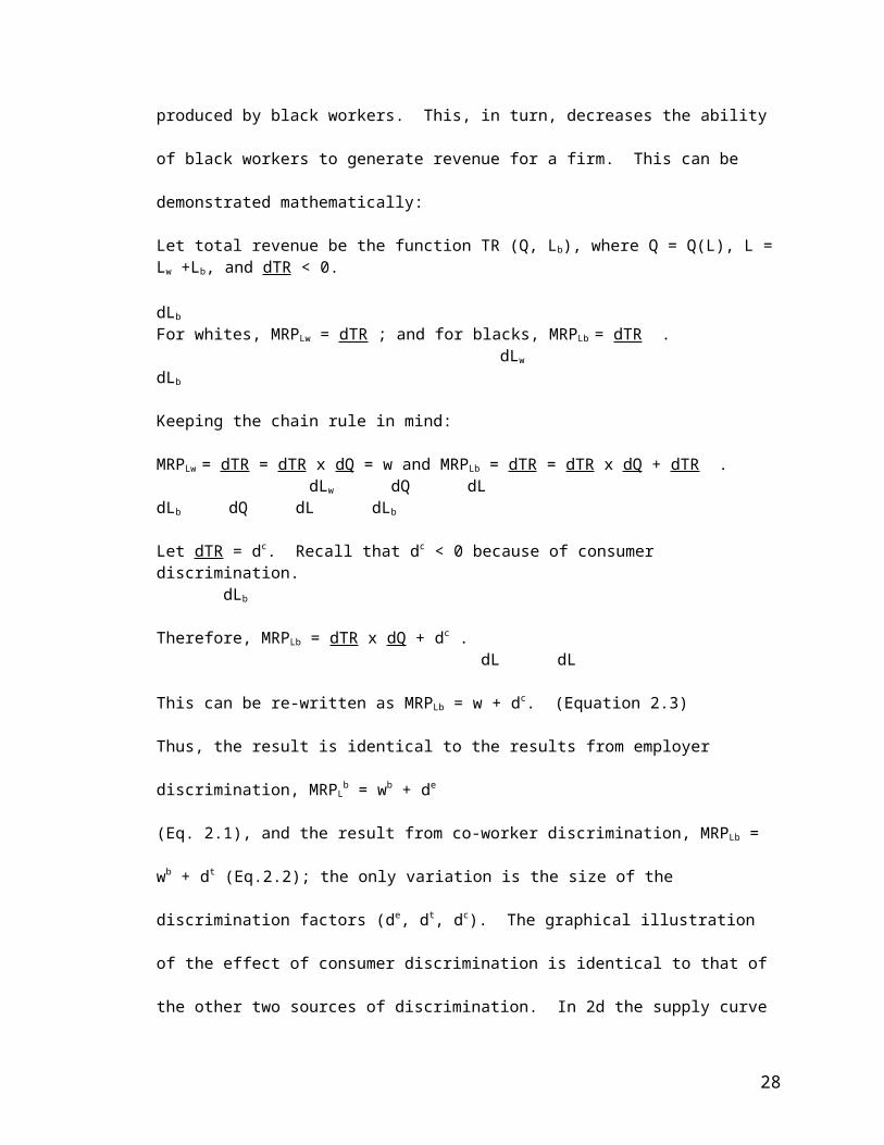
3) In the case of consumer discrimination, consumers are averse to purchasing goods produced by

black workers. As a result, consumer discrimination reduces the demand for output/goods

produced by black workers. This, in turn, decreases the ability of black workers to generate

revenue for a firm. This can be demonstrated mathematically:

Let total revenue be the function TR (Q, Lb), where Q = Q(L), L = Lw +Lb, and dTR < 0. dLb

For whites, MRPLw = dTR ; and for blacks, MRPLb = dTR . dLw dLb

Keeping the chain rule in mind:

MRPLw = dTR = dTR x dQ = w and MRPLb = dTR = dTR x dQ + dTR . dLw dQ dL dLb dQ dL dLb

Let dTR = dc. Recall that dc < 0 because of consumer discrimination. dLb

Therefore, MRPLb = dTR x dQ + dc . dL dL

This can be re-written as MRPLb = w + dc. (Equation 2.3)

Thus, the result is identical to the results from employer discrimination, MRPLb = wb + de

(Eq. 2.1), and the result from co-worker discrimination, MRPLb = wb + dt (Eq.2.2); the only

variation is the size of the discrimination factors (de, dt, dc). The graphical illustration of the

effect of consumer discrimination is identical to that of the other two sources of discrimination.

In 2d the supply curve for black labor shifts up by dc. As a result, the market equilibrium values

in market equilibrium are identical as well: the quantity of labor demanded equals the quantity of

labor supplied (Lw + Lb); the new equilibrium wage received by whites rises, ww** > w*; the

quantity of white labor increases from Lw* to Lw

**; new equilibrium wage for blacks, wb**, falls,

wb** < w* where wb

** = ww** - de; the quantity of black labor decreases from Lb

* to Lb**. (Of

course, if dc is larger than dt or de, the magnitude of the declines would be larger. However, the

general pattern remains the same for all three sources of discrimination.)

18

MLB, and professional sports leagues in general, represent a unique market in which

consumers pay to observe the process of production. In other markets, goods are not produced

with such direct level of consumer contact. Thus, it is possible that consumer discrimination has

a larger effect in MLB than in other markets. Furthermore, competitive forces will not eliminate

consumer discrimination over time. The competitive forces in the baseball market are not

directly experienced by the consumers, and have no effect on their discrimination preferences

which reduce the MRPL of black players. In fact, one could argue that cities with racist fans are

more likely to have an all white team and that cities with the least racist fans will have more

integrated teams. Due to its possible persistence, consumer discrimination seems more likely to

be responsible for wage and employment gaps than employer and co-worker discrimination.

This section will now review past economic studies that attempt to identify and measure

employer, co-worker, and consumer discrimination in baseball.

Literature Review

As mentioned in the previous chapter, labor markets in professional sports provide a well

suited laboratory for studying discrimination because performance data is readily accessible.

Hard performance data allows one to estimate an individual’s marginal product of labor (MPL)

and investigate the possibility of discrimination. Past studies have employed a wide array of

analytical methods in order to investigate discrimination and attempt to isolate the source (either

employer, co-worker, or consumer). In general, previous studies can be grouped into six main

categories: 1) wage and bonus differentials; 2) performance and promotion differentials; 3)

positional segregation; 4) attendance levels; 5) all-star voting trends; and 6) pricing in the

baseball memorabilia market.

Wage and Bonus Differentials

19

If there were significant discrimination in the MLB player market, one would expect to find a

wage differential for given levels of productivity: a lower wage for minority players who were

equally as productive as white players. In general, little evidence of salary discrimination has

been found in baseball. Using the same sample of 148 players in 1968, Scully (1974) and Pascal

and Rapping (1972) found no evidence of salary discrimination against black hitters (non-

pitchers).15 Seven further studies, Medoff (1975a, 1975b), Mogull (1981), Cymrot (1983, 1985),

Raimondo (1983), and Kahn (1989) also report insignificant salary discrimination against black

baseball players. Scully (1973) and Gwartney and Haworth (1974) found significant

discrimination in signing bonuses paid to players in the 1950s and 1960s (20% of whites received

bonuses over $20,000 while only 8.6% of blacks did). This differential is striking given the

superior performance of black players during that time. It is interesting to note that Christiano

(1986, 1988) found significant salary discrimination against white players in 1977 and 1987. In

1977, a white player received a salary 4.6% smaller than that of an equally productive non-white

player; in 1987, a white player received a salary 17% smaller. In summary, there is little or no

empirical evidence salary discrimination against blacks.

Performance and Promotion Differentials

If discrimination exists in the market, one can infer that an average non-white player will have

better performance statistics than a white player. Recall that economic theory states that an

individual employer hires a minority worker only when their MRPL exceeds the wage by the

discrimination factor; either de, dt, or dc depending on the source of discrimination. Given that

MRPLw = w, it follows that for players already hired MRPLb > MRPLw on average. Pascal and

Rapping (1972) and Scully (1974) found that black players in 1968 had significantly better

performance statistics at all positions controlling for differences in lengths of career. Pascal and

Rapping focused solely on batting averages for hitters, and games won for pitchers, while Scully

looks at several more performance statistics for hitters and pitchers (such as slugging percentage,

15 Furthermore, these studies reported black pitchers actually earned more than their white counterparts after accounting for performance.

20

ERA, strikeouts etc.). Furthermore, Gwartney and Haworth (1974) and Hanssen (1998) found a

sizeable positive relationship between the number of black players in the starting lineup and

winning percentages in the 1950s and beyond. Gwartney and Haworth reported that an additional

black player resulted in an additional 3.75 wins per year, 2 wins per year after controlling for

team quality. Hanssen’s analysis extended beyond the 1950s and found that this effect

diminished over time. He found that an additional black player resulted in nearly 6 additional

wins per season in 1950, while in 1984 less than 1 win resulted.

The theoretical justification for performance differentials in the presence of discrimination is

reinforced by evidence seen from the promotion of players to the major leagues. In this manner,

discrimination takes a different form through which blacks have more difficulty being promoted

to the major leagues, the so-called glass ceiling. Bellemore (2001) looked at the promotion of

Hispanic and black players from the AAA minor leagues to the major leagues. In the 1960s and

1970s, he found that blacks were 9.3% less likely to be promoted than a white player with

comparable performance, and a Hispanic player was 15.6% less likely than an equally productive

white player. Significant discrimination persisted in the 1990’s toward black players as 8.1%

were less likely to be promoted; in contrast, Bellemore found that discrimination toward

Hispanics disappeared completely. It is interesting to note that the degree of discrimination

towards Hispanic players became insignificant during the early 1990s when MLB expanded into

markets with a large proportion of Hispanics (Miami, Tampa Bay, Phoenix); such a result is

consistent with Becker’s model that entry/expansion would decrease employer discrimination.16

Positional Segregation

16 This result is also consistent with consumer discrimination. One would expect cities with a large Hispanic population to be less discriminatory toward Hispanics than cities with a small one. Therefore, it seems plausible that Hispanics players would be promoted more frequently to cities with a large Hispanic population. That is, there will be natural allocation of Hispanic players to cities who do not discriminate against Hispanics.

21

Discrimination can lead to segregation of several forms: white only and non-white only

leagues, white only and non-white only teams within a single league, and specific playing

positions that are exclusively held by white players within integrated teams and leagues. Several

studies have found positional segregation in MLB with most reporting that blacks are

overrepresented at outfield and first base and underrepresented at pitcher. Scully (1973) reported

that 53% of all outfielders were black while only 9% of pitchers were black. Scully also found

that blacks were underrepresented at catcher. Pascal and Rapping (1972), Hill and Spellman

(1984), and Christiano (1988) found similar results. Furthermore, Medoff (1986) noted that black

representation is lowest for positions that require the most training and have the highest

equipment cost: pitcher and catcher. The positions of catcher and pitcher also have the most

responsibility/team leadership of any position. Thus, it appears that black players are

discriminated against being team leaders.

Economists have also looked at the hiring of non-white general managers and coaches in an

attempt to measure discrimination. Singell (1991) found that blacks are significantly less likely

to be hired into managerial positions than whites, even after controlling for experience and

previous winning team percentages.

All-Star Voting Trends

Several studies have looked at all-star voting results in an attempt to measure discrimination,

specifically consumer and co-worker discrimination. Broadly speaking, MLB has used two

methods to choose starting lineups for the All-Star game: player voting and fan voting. The

hypothesis is that a discriminating fan or teammate will express their taste for discrimination by

voting for white players even though they performed worse than non-white players. Hanssen and

Anderson (1999) found evidence that discrimination toward black players has decreased

significantly over time. They reported that white players received more fan votes than equally

qualified blacks during the 1970s; however this differential declined sharply and there was no

difference in the 1980s. Interestingly, the trend actually reversed in 1996 as black players

22

received more votes than equally qualified whites. Moreover, Hanssen and Anderson reported

insignificant voting discrimination toward Hispanics over all years. Depken and Ford (2001)

confirm these results.

Hanssen performed another study concerning all-star voting in an effort to separate co-worker

and consumer discrimination. In Hanssen (2001), he analyzed all-star voting in 1969, a year in

which only players voted, and in 1970, when the process returned to only fans voting. (The

system now has fans vote and the managers/players vote for the reserves.) Hanssen argued that

by doing so one can infer if players (co-workers) exhibited more discrimination than fans, or

vice-versa. After controlling for performance, he found that baseball players were more

discriminatory than fans.17

Pricing in Baseball Memorabilia Market

More recently there has been a trend for economists to test for discrimination by analyzing the

baseball memorabilia market. These studies provide a test for the presence of consumer

discrimination. Results from this type of test should be taken with extreme caution as the

memorabilia market is shallow, in the sense that far fewer people participate in the market for

memorabilia then attend baseball games. (Furthermore, the market consists of a large percentage

of young people who do not have any income, and a small percentage of individuals with very

high incomes and inelastic demand curves who dominate the market for high-priced

memorabilia.) Thus, tests of the memorabilia market are not totally reflective of the typical

consumption of the product of baseball as entertainment.

17 Another test for discrimination examines the Hall of Fame voting outcome by the Baseball Writer’s Association of America’s (BBWWAA). These studies do not find significant evidence of discrimination. Findlay and Reid (1997), Dessler (1999), and Jewell et al. (2002) all found limited evidence of discrimination against blacks or Hispanics in Hall of Fame voting. They concluded that the magnitude of the discrimination is so small that it would not alter the racial composition of the Hall of Fame. That is, no player that would be predicted to get into the Hall of Fame based on career performance was left out because of his race. Furthermore, Desser et al. (1999) reported that there is limited evidence of discrimination against blacks and Hispanics in the nomination process. And Jewell et al. (2003) concluded there is no evidence of discrimination as both blacks and Hispanics do not wait longer to be elected into the Hall than equally productive white players.

23

Studies concerning pricing in memorabilia markets provide conflicting results. Nardinelli

and Simon (1989) found significant evidence of discrimination when they analyzed at the prices

(in terms of 1989 dollars) of a set of cards issued in 1970. Overall, they reported that cards of

nonwhite hitters sold at a price 10% less than those of whites with equal ability (black players’

cards sold at 6.4% less and Hispanic players’ cards at 17% less). And cards of non-white pitchers

sold at 13% less than those of white pitchers. Anderson and La Croix (1991) reported similar

results in their analysis of a 1977 set of baseball cards. However, Gabriel et al. (1995) found no

evidence of discrimination in the prices of their sample rookie baseball cards from 1984-1990.

They suggest that this result could be caused by the fact that they studied cards of active players,

not retired ones. They state that the ethnicity of a player could influence a consumer’s future

expectation of the player’s performance, which in turn influences the price of the baseball card.

That is, race has no significant effect on the price of a card at the start of the player’s career; but

by the time a non-white player retires, his card is devalued to that of an equally productive white

player due to the elimination of any future expectations on performance. Gabriel et al. confirm

their results of no discrimination for an earlier sample of cards in Gabriel et al. (1999). They

looked at 1983 and 1994 price data for rookie cards from 1974-1982 and reported no difference

between the prices of cards based on race.

Attendance Levels

Perhaps a more accurate way to gauge the extant of consumer discrimination is to examine the

relationship between the number of non-white players on a team and fan attendance levels. The

proposition is that more non-white players would decrease fan attendance because fans have an

aversion to consuming output produced by minorities. Scully (1974) first tested this theory by

looking at fan attendance for games in which the starting pitcher was black. He argued that

pitchers are rotated on a regular basis and information about which pitcher will be starting are

announced publicly several days before each game. Therefore, fans can discriminate about which

games to attend games based on the race of the starting pitcher. Scully estimated the average

24

home attendance of 57 National League pitchers over the 1967 season and found that, on average,

2,000 fewer fans attended games pitched by blacks than those pitched by whites. Scully included

a dummy variable for each city to negate intercity variation. While he did not control for pitcher

quality, he pointed out that black pitchers performed better than white pitchers, on average.

Other studies have expanded on Scully’s analysis of black pitchers to the effect of the number

of total black players on a team (usually just in starting lineup, but sometimes on bench as well).

These studies have produced contrasting results. Gwartney and Haworth (1974) found that the

number of black players on a team had a significantly positive effect on annual attendance over

the 1950s: between about 16,000 and 29,000 fans per year after controlling for team winning

percentage. The authors suggest that either the superstar effect or an increase in black fan

attendance, enough to offset the decrease in attendance by whites, could explain their results.

However, Noll (1974) concluded that the latter explanation is not viable. In contrast to Gwartney

and Haworth, Hanssen (1998) found a significant negative relationship between black players in

the starting lineup and fan attendance. Hanssen also reported that fan attendance for American

League teams decreased by much more than attendance for National League teams in response to

the number of black players on the team. He suggests that the difference in fan preferences

between leagues could help explain why the American League integrated significantly slower

than the National League. The contrasting results between Gwartney and Haworth and Hanssen

might be explained by their different empirical methods: Gwartney and Haworth looked at

cumulative games played by black players on a team while Hanssen looked only at the number of

black players on a team. Furthermore, Hanssen included a variable for the percent of the

population in each team’s Standard Metropolitan Statistical Area that is black, while Gwartney

and Haworth did not. Gwartney and Haworth may have had an omitted variable bias in which

their positive coefficient was overstated because it captured the effect of the of percentage of the

SMSA population that was black. But such an argument assumes that the effect is positive; this

25

assumption is debatable. The most likely reason for the contrasting results is that the authors

used different multipliers in determining how an additional win affected fan attendance.

This paper will now turn to its two empirical studies; the first of which falls under the category

of performance differentials, the second under fan attendance.

Chapter 3: Empirical Methods, Results, and Analysis

This section examines evidence of both co-worker and consumer discrimination. Co-worker

discrimination is analyzed by estimating the relationship between a team’s winning percentage

and the relative employment of black and Hispanic players. Consumer discrimination is analyzed

by evaluating the relationship between fan attendance and the employment of black and Hispanic

players. Both analyses consider all major league teams from 1950 to 1999.18

Co-Worker Discrimination

To explore the existence of co-worker discrimination, I estimated the relationship between

annual winning percentages and the relative employment of black and Hispanic ballplayers. To

control for the ability of players on the team, I use the hitting statistic, On Base Plus Slugging

(OPS), and the pitching statistic, Earned Run Average Plus (ERA+). OPS equals the sum of On-

Base Percentage and Slugging Average; the deviation of a team’s OPS from the league mean (AL

or NL, accordingly) is used in this study. ERA+ is equal to the league average ERA divided by

team ERA.19 Note that both of the measures of team performance, deviation of OPS and ERA+,

reflect a team’s level of performance relative to other teams in its league for each year.20 I am

considering time series data; therefore, I will account for the possibility of autocorrelation. In

addition, I use a league dummy variable that equals 1 for the American League and 0 for the

18 Teams that relocate to a different city are treated as a different team.19 On-Base Percentage equals [(Hits + Walks + Hit-By-Pitch) divided by (At Bats + Walks+ Hit-By-Pitch + Sac Flys)]. Slugging Average equals [Number of (Singles + [2 x Doubles] +[ 3 x Triples] + [4 x Home Runs]) divided by At-Bats]. Earned Run Average equals [(Number of Earned Runs x 9) divided by (Number of Innings Pitched)].20 The argument is that relative performance is more important than absolute performance due to the fact that teams necessarily compete against each others for wins. These statistics are generally regarded as the best measures of hitting and pitching.

26

National League to account for inter-league differences which are not encapsulated by the other

explanatory variables.21

Table 3.1Variable Expected coefficient

Deviation in OPS PositiveERA+ Positive

Only black and Hispanic “starters” are counted; both hitters and pitchers are included.

‘Starting’ hitters are classified as those who played in the most games at a given position for their

team over the season. ‘Starting’ pitchers are those who pitched at least 100 innings over the

season.22 The data set from Hanssen (1998) and pictures from official team websites were used to

categorize ‘black’ players. Hispanic players are defined as those born in a Latin American

country or those with a Hispanic surname.23 Relative employment is measured as the deviation in

the number of black ‘starters’ and the deviation in the number of Hispanic ‘starters’ from the

league means. In addition, I included a squared term for each to allow for nonlinearities.

It is assumed that relative measures of performance and employment affect winning more

directly than absolute levels because teams compete against other teams in the same league for

wins.24 The squared term is included because co-worker discrimination could lead to segregation

of teams – if co-worker discrimination exists, owners would react by building a team that would

be predominantly white or predominantly black. The squared term allows us to test the

hypothesis that a predominantly white team or a predominantly minority team will be more 21 Instead of using a dummy variable to account for league differences, one could use an interaction term that multiplied the relative employment of black and Hispanic players times a league dummy. Such interaction variables present the differences in the league specific means and league specific rates of increase in black and Hispanic starters. Several regressions were performed using interaction variables instead of league dummies; but none of their coefficients for the interaction terms were significant. (The coefficients of the other variables were qualitatively similar.)22 The choice of 100 innings is arbitrary. However, an analysis of the data indicates that only pitchers in the starting rotation and primary relievers pitched more than 100 innings.23 Players with a Hispanic surname are categorized as Hispanic because they are generally labeled/associated as being Hispanic by both co-workers and consumers; therefore, discriminatory preferences would still apply even though they were born within the US.24 However, if absolute levels are used instead, the results are qualitatively similar. Furthermore, it is understood that with the start of interleague play in 1997, teams now compete against teams in the other league for wins. But interleague play lasts for only two weeks each season; thus, teams predominantly compete only against teams within the same league.

27

successful than an integrated team. In other words, the hypothesis posits that segregation has a

parabolic effect on winning percentage. Including this squared term allows me to test for this

parabolic influence.

Table 3.2 Summary Statistics for Variables from Co-Worker Discrimination Regressions (N=1142)Variable Definition Mean Std. Dev. Min. Max.winpercp Winning percentage x 100| 50.0 7.39 24.84 71.15

devops (Team OPS – League Average OPS) 0 .033 -.156 .101

eraplus (League Average ERA) / Team ERA 0 .045 -.190 .149

blackstart # of Blacks in Starling Lineup 2.92 1.57 0 6

leaguemeanblacks League Average # of Blacks inStarting Lineup

2.92 1.01 .25 4.12

devblackststart (blackstart – leaguemeanblacks) 0 1.20 -2.75 3.25

devblackststartsq (blackstart – leaguemeanblacks)2 1.45 1.68 0 10.56

hispanicstart # of Hispanics in Starting Lineup 1.91 1.48 0 8

leaguemeanhispanics League Average # of Hispanics in Starting Lineup

1.91 .716 -3.625

3.71

devhispanistartt (hispanicstart – leaguemeanhispanics)

0 1.30 -3.625

4.92

devhispanistartsq (hispanicstart – leaguemeanhispanics)2

1.70 2.55 0 24.29

Figure 3.1

Percent of White, Black, and Hispanic Starters from 1950-1999

0102030405060708090100

1950 1955 1960 1965 1970 1975 1980 1985 1990 1995

Year

Perc

ent

Hispanic

Black

White

This model is designed so that evidence of co-worker discrimination is given by the

coefficients for the deviations of black and Hispanic players from the league means and the

28

deviations squared. The hypothesis is that the addition of a black or Hispanic player affects

“team chemistry” in a way that influences how a team can turn its performance into victories.

Team chemistry is defined as all non-performance team interactions that impact the ability to win

(such as team camaraderie, clubhouse relations, practice behavior, etc.).25 Because teams

compete against other teams within the same league for victories, it is appropriate to use relative

measurements. The impact of co-worker discrimination on team chemistry is expressed by the

coefficients of the variables for the deviation of black and Hispanic players from the league

means, and these deviations squared. For example, a negative coefficient for the deviation of

black players from the league mean implies that teams above the league mean in black starters

have poorer team chemistry which in turn hampers their ability to win games. Thus, a negative

coefficient for the deviation of black or Hispanic players from the league mean implies co-worker

discrimination. Furthermore, a positive coefficient for the deviation squared term implies that

teams that are predominantly all black/all Hispanic or predominantly all white gel better and win

more games. That is, a higher degree of segregation leads to more wins; hence, a positive

coefficient implies co-worker discrimination. (The result of segregation in a market with co-

worker discrimination is consistent with economic theory.)

The results from Model 1 are shown in table 3.3 and are separated into the Early Years and the

Later Years. The Early Years are defined as 1950-1955 for black players and 1950-1963 for

Hispanic players. The end of each range represents 8 years after the pioneer of each race entered

MLB, Jackie Robinson in 1947 and Roberto Clemente in 1955.26

Insert Table 3.3

25 It is assumed that white players do not express their discriminatory feelings directly through lowered individual productivity. This assumption seems reasonable because white players who decreased their productivity due to their discriminatory preferences faced the possibility of a decreased salary in the future or replacement by another player, possibly a black or Hispanic player, with higher productivity. 26 Specific analysis of these years was performed after initial regressions suggested a unique effect for these periods. The ends of each range were chosen in an effort to normalize the analysis in terms of the number of black and Hispanic players in MLB.

29

Insert Table 3.3

The results for the early years are reported in Regressions 1-4. The performance statistics were

positive and significant at the 1% level. The coefficient for hitting performance, deviation of ops

(devops), ranged from 125.44 to 142.256 and that of eraplus ranged from 40.95 to 47.045. This

suggests that an increase of .10 in a team’s OPS relative to the league mean resulted in about 20

30

more wins a year, and an increase of .10 in a team’s ERAplus resulted in roughly 7 additional

wins.

The coefficient of the linear deviation term provides a surprising and interesting result.

Instead of being negative, the coefficient estimates were positive in the Early Years. This

suggests that there was positive co-worker discrimination toward both black and Hispanic

ballplayers during this period. In other words, black and Hispanic players produced more wins

after accounting for their batting and pitching ability, suggesting that their presence on the team

influenced team chemistry in a positive way. Teams with one more black starter relative to the

league mean increased winning percentage by .8836 percentage points or 1.36 wins a year.

Similarly, teams with one more Hispanic starter relative to the league mean increased winning

percentage by .4282 percentage points or .67 games a year.27 It is important to note that while

these effects are statistically significant, their magnitudes are very small. Moreover, there were

very few black and Hispanic starters in the Early Years; so it is unlikely that any team was more

than one black or Hispanic starter away from than the league mean.

This surprising result can be reconciled when one considers the characteristics of the black and

Hispanic ‘pioneers’ in MLB. Undoubtedly, these pioneers were very talented players, but they

were not just chosen for their baseball abilities. Branch Rickey, the President and General

Manager of the Brooklyn Dodgers, was very candid in why he chose Jackie Robinson to break

the “color” barrier in 1947. In his own words, Rickey wanted “a ballplayer with guts enough not

to fight back." Rickey wanted to integrate the major leagues, and was looking for a player who

could withstand the hostility he would face. After several years of study, Rickey concluded that

Robinson was this player. In addition to his baseball abilities, Robinson was exceptionally

mature. Rickey believed that Robinson had the ability to cope with all the pressures that he

27 From 1950 through 1960, each team played 154 games per year. Since 1961, each team has played 162 games. The calculation given for Hispanic co-worker discrimination assumes a 154 game schedule. Since the range extends to 1963, a trended calculation was performed that yields an increase of .67 games a year. All future calculations that describe the impact on number of wins are also trended calculations that take into account the change in the number of games played per year.

31

would face as the first black player. A similar argument can be made for many of the other

pioneers: they were exceptionally mature individuals who had strong interpersonal and leadership

skills in addition to being highly skilled athletes. Therefore, they knew how to get along with

others and how to be team players. The regression results could be explained by the hypothesis

that their addition did not detract from team chemistry; in fact, it enhanced it, resulting in more

victories.

When the whole time period is studied at once, as seen in Regressions 5 and 7, the coefficients

of the linear deviation terms for both black and Hispanic starters are insignificant. Recall that the

coefficients for the linear deviation terms had small, but significant positive values for the Early

Years. It is possible that the Early Years’ values cancel out any significant negative coefficients

for the Later Years; that is, the results from the Early Years could drive the insignificant results

evident in Regressions 5 and 7. Therefore, one could argue that the coefficient for the linear

deviation of black starters is significant and negative after 1955, while that of Hispanics is

significant and negative after 1963. Regressions 6 and 8 test this argument and demonstrate that

the Early Years did not drive the previous results; the coefficients for the linear deviation terms

are both insignificant. The linear deviation terms for both black and Hispanic players are also

insignificant when isolating the years 1960-1979, and 1980-1999. (Reg. 9-10 and 11-12) These

results support the conclusion that that the Early Years’ values did not drive the insignificant

results evident in Regressions 5 and 7.

Remember that this model provides a differential discrimination treatment through both a

linear deviation variable and a deviation squared variable. It was just mentioned that the linear

deviation term was significant in the Early Years but insignificant in the Later Years. The focus

is now shifted to the deviation squared term to analyze the presence of a ‘segregation effect’ as

evidence of co-worker discrimination. In the Early Years, the coefficients for both the deviation

squared term for blacks and Hispanics were insignificant. For the whole time period, 1950-1999,

the coefficient for Hispanics is insignificant but the coefficient for black players is .2026 and

32

significant at the 5% level (Reg. 5 and 7). This result implies that teams with a higher degree of

segregation enjoyed somewhat greater success from 1950-1999. This may suggest the presence

of both white and black co-worker discrimination. Whites may like to play with whites;

therefore, the addition of blacks on a “predominantly” white team reduces winning percentage.

Similarly, blacks may like to play with blacks; therefore, adding white players to a

“predominantly” black team reduces winning percentage. The ‘segregation effect’ decreases over

time as the magnitude of the coefficient for the deviation squared term declines to .190 for the

1960s and 1970s, and is insignificant for the 1980s and 1990s (Reg. 13 and Reg. 14), in regard to

black starters.

A fixed effects model was also run for both black and Hispanic players to control for

remaining cross-team or city differences. The results are presented by Regressions 23 and 24 and

are qualitatively equivalent to the results from Regressions 5 and 6. The fixed effects model

controls for city specific characteristics that are not captured by the explanatory variables (such as

religious affiliation, racial demographics, political ideologies, etc.). The fact that the fixed effects

model did not significantly alter the results is not surprising as city characteristics are not likely to

effect team performance.28

Consumer Discrimination

To examine the existence of consumer discrimination, I will estimate the relationship between

annual fan attendance and the employment of black and Hispanic ballplayers. For city controls, I

include the population and per-capita income of the relevant standard metropolitan statistical

area,29 and the percentages of the relevant SMSA’s population that are black and Hispanic.30 Two

dummy variables were also included to indicate the existence of a competing MLB franchise or a

28 It is possible that some city characteristics directly effects local team support. If winning is a function of team support (not an unreasonable assumption), then one could argue that certain city characteristics do influence a team’s ability to win. As a result, one would expect the fixed effects model to produce to different results. 29 Teams from the same city share the same SMSA data.30 These variables are included to see if black and Hispanics are more or less likely to attend baseball games than whites.

33

professional team in a different sport in the SMSA. For team controls, I incorporate the team’s

winning percentage.31

Table 3.4Variable Expected coefficient

Population PositivePer Capita Income Positive

Percentage of Population Black UncertainPercentage of Population Hispanic Uncertain

Other MLB Franchise NegativeOther Professional Sports Team Negative

Winning Percentage Positive

Table 3.5 Summary Statistics for Variables from Consumer Discrimination Regressions (N=1142)Variable Definition Mean Std. Dev Min Maxattend Annual attendance

(in 1,000’s)1,558.469 736.3081 247.13 4483.35

pop SMSA Population(in 1,000’s)

3,579.846 2,537.96 270.42 10,402.00

percapitaincome SMSA Per Capita Income (in $1,000’s)

9.68 7.33 6.43 36.21

percblack % of SMSA Pop. that is Black 14.16 6.77 .61 28.91

perchispanic % of SMSA Pop. that is Hispanic 7.92 8.98 .41 44.56

othermlbteam Other MLB Team .17 .38 0 1othersportteam Other Professional Sports Team .75 .42 0 1

winpercp Winning Percentage x 100 50.00 7.38 24.84 71.15

blackstart # of Blacks in Starting Lineup 2.92 1.57 0 6hispanicstart # of Hispanics in Starting Lineup 1.912 1.48 0 8

Finally, the numbers of black and Hispanic players in the starting lineup are entered as the

primary variables of interest.32 If fans preferred white players to black players or white players to

Hispanic players, ceteris paribus, the effect of these variables will be negative. That is, a

negative regression coefficient for these variables would indicate consumer discrimination; fans

31 The assumption is that the fans receive extra utility from attending games in which the home team wins. All things equal, more winning is preferred to less; therefore, one would expect more fans to attend baseball games as their team produces more victories.32 This is in contrast to the deviation from the league mean measurements used in the previous model that analyzed co-worker discrimination. Absolute measures are more appropriate here because fans do not consider how mixed the team is relative to the league mean in making their decision to attend a game.

34

attend fewer games, their demand for output (baseball entertainment) produced by black and

Hispanic workers (players) decreases because of their discriminatory preferences.

One variable that is virtually impossible to obtain before 1995 is ticket prices. This is

unfortunate because ticket prices are part of the demand function for fan attendance. Therefore, I

will not be estimating a “true” demand function; instead, I will be estimating a reduced form

equation. The assumption is made that profit-maximizing prices are chosen. This can be

represented mathematically:

Attendance = Q = β0 + β1 Price + β2 Exogenous Variables; β1 < 0

Q = β0 + β1P + β2X β1P = Q – β0 – β2X P = _Q_ – _β0_ – _β2X_ β1 β1 β1

TR = PQ = _Q 2 _ – _β0Q_ – _β2XQ_ β1 β1 β1

π = TR – TC d π = _2Q_ – _β0_ – _β2X_ – dTC = 0dQ β1 β1 β1 dQ

_2Q_ = _β0_ + dTC + _β2X_ β1 β1 dQ β1

Q = _β0_ + _ β 1_dTC + β2X; assume, TC = 0. 2 2 dQ dQ

In this reduced form model, the estimated parameters indicate the change in the profit-

maximizing quantity of attendance for each unit change in the Exogenous Variables. Note that

the coefficient for Exogenous Variables in the reduced form equation, β2, is the same as that in

the true demand function. Therefore, the coefficients from these regressions will have the same

interpretative function as those from the true demand equation. That is, the results that are

obtained, should have the same sign and magnitude of the values from the true demand function.

Table 3.6 shows the results from model 2. Looking at the time period as a whole (1950-1999),

in regard to black players, the coefficients for the city control variables are all significant with the

predicted sign, except for percblack and othersportsteam.33 Regression 1 demonstrates that

33 The insignificance of percblack suggests that there was no difference in the affinity for baseball between blacks and whites when analyzing the time period as a whole. However, the coefficient for percblack is negative and significant in the 1950s (Reg. 3) and 1970s (Reg. 7). This suggests that blacks were less

35

100,000 more people in the SMSA increases annual attendance by 9,800, a $1,000 increase in

per-capita income improves attendance by 55,180, and the presence of another MLB team in the

city decreases attendance by 523,480 annually. In addition, winpercp, which controls for team

quality, was also significant with the expected sign; a 10 percentage point increase in winning

percentage (roughly 16 more wins a year) enlarges yearly attendance by 387,200.

Regression 1 suggests that there was no consumer discrimination against black starters;

instead, it implies that there was slight positive (and statistically significant at the 5% level)

discrimination toward black starters. From 1950-1999, on average, the addition of one more

black player in the starting lineup resulted in an increase of fan attendance by 20,750 per year (or

around 130 per game)34. Upon further inspection of the time period, the coefficient for blackstart

is positive and significant for the 1950s and 1960s, and insignificant for the 1970s, 1980s, and

1990s. (Reg.3, 5, 7, and 9) Thus, there is evidence of positive consumer discrimination in the

1950s and 1960s and no discrimination from 1970 onward. In the 1950s an additional black

starter increased annual attendance by 93,390 (or 583 a game) (Reg. 3), and in the 1960s by

roughly 95,000 per year (or 594 a game) (Reg. 5). The result that black players increased

attendance levels in the 1950s after controlling for team quality (existence of positive consumer

discrimination) is consistent with the findings from Gwartney and Haworth (1974).

Insert Table 3.6

likely to attend baseball games than whites during these time periods. 34 All per game calculations are performed using a linear trend model accounting for the increase in the number of games played per year from 154 to 162 in 1962.

36

Insert Table 3.6

Insert Table 3.6

One possible explanation for the positive relationship between fan attendance and black

starters in 1950s and 1960s is the superstar effect. The first black players in the MLB were much

better than the average white ballplayer. These pioneers were among the league leaders in most

statistical categories. The high quality of early black players is supported by the large number of

Rookie-of-the-Year Awards and Hall of Fame enshrinements that they obtained.35 The superstar

35 Between 1949 and 1962, eleven Rookie-of-the-Year Awards went to black players. Furthermore, all NL teams, except the Cardinals and the Phillies, featured at least one black player headed for the Hall of Fame.

37

effect hypothesizes that one reason fans attend ballgames is to see great individual performances.

Therefore, fan attendance increased with the addition of the early black players because of their

superb individual skills, over and above their contribution to the team’s winning percentage. The

superstar effect is also consistent with the indication of the disappearance of positive consumer

discrimination over time. It is well-documented that performance differentials between black and

white ballplayers narrowed over time (Pascal and Rapping, 1972). The average black player after

1970 was not as good, relative to white players, as the average black player in the 1950s and

1960s. Thus, one can infer that the magnitude of the superstar effect shrunk over time because

the average new black player was less likely to be a superstar.

Another possible explanation is that breaking the color barrier was a monumental event that

generated a considerable stir among the baseball community, and society in general. The

‘hoopla’ associated with this event sparked general curiosity/interest among individuals who

ordinarily did not attend baseball games. Thus, people who did not normally attend games began

to do so in order to witness the pioneer black players and the newly integrated MLB because of

the hype surrounding them. This hypothesis is also consistent with the disappearance of positive

consumer discrimination over time as the hype surrounding the integration of baseball decreased

gradually. The addition of black players shifted from being a novelty, to being the norm;

therefore, fans who attended games for the novelty of watching black players, stopped attending

games.

Finally, the results could be explained by the elimination of the Negro Leagues. When the

Negro Leagues collapsed, the only place for black baseball enthusiasts to watch black

professional ballplayers was in MLB. Therefore, fans who previously attended Negro League

games in order to watch black ballplayers started attending MLB games. Gwartney and Haworth

(1974) provided a similar hypothesis that an influx of black fans due to the elimination of the

Negro Leagues explains their results. However, Noll (1974) concluded that this hypothesis was

38

not valid because attendance levels increased by more than the number of potential newfound

black MLB fans.36

In regard to Hispanic players, from 1950-1999 (Reg. 2), the coefficients for the city control

and team control variables are qualitatively similar to those in the analysis of black starters in

Regression 1. The only difference is that the coefficient for perchispanic is significant in

Regression 2. (Whereas the coefficient of percblack was insignificant in Regression 1.) More

importantly, Regression 2 shows no significant relationship between the number of Hispanic

starters and attendance levels; the coefficient for hispanicstart is insignificant. There is no

indication of consumer discrimination in terms of Hispanic starters during this time period.

Upon further inspection of the time period, the coefficient for hispanicstart is negative and

significant for the 1950s, insignificant for the 1960s and 1970s, and positive and significant for

the 1980s, and 1990s (Reg. 4, 6, 8, 10). These results suggest that there was small consumer

discrimination against Hispanic players in the 1950s – one additional Hispanic starter decreased

annual attendance by 40,850 (or 255 a game) (Reg. 4); and positive consumer discrimination

toward Hispanic players in the 1980s and 1990s - an additional Hispanic starter increased

attendance by 30,240 (or 189 a game) (Reg. 10).37

None of the three posited explanations for the results concerning black starters seem plausible

in regard to the relationship between attendance and Hispanic starters. Thus, a fixed effects

model was run for both black and Hispanic starters in order to further understand the implications

of these results. The fixed effects model controls for cross-city differences; these differences are

assumed to be stable over time. Taking into account cross-city differences seems important for

investigating consumer discrimination because some cities are more racist than others. A city’s

geographical location, political and religious culture, etc. may influence the discriminatory

preferences of baseball fans. These characteristics are not captured by the explanatory variables

36 The negative coefficient for percblack in the 1950s, and the insignificant coefficient for the 1960s, support Knoll’s conclusion that the increase in annual attendance was not caused by a sudden influx of black fans. 37 Note that this coefficient is barely significant at the 10% level.

39

in the OLS regressions. Thus, a fixed effects model seems appropriate because it controls for

these city-specific characteristics that are not captured by the included city-specific variables.38

The results from the fixed effects model are presented in Table 3.7.

Looking at the time period as a whole, in regard to black starters (Reg. 11), the coefficients for

the city control variables are qualitatively similar (significant with the predicted sign) to those in

Regression 1 of the OLS estimations, except that the coefficient for percblack is now positive and

significant.39 In addition, the coefficient for winpercp in is consistent with that of Regression 1.

It is important to note that the coefficient for blackstart is insignificant in Regression 11. This

contrasts with the positive and significant result from Regression 1. When breaking the time

period down into decades, the coefficient for blackstart is insignificant for the 1950s, 1970s,

1980s, and 1990s, but is positive and significant for the 1960s (Reg. 13, 15, 17, 19). The

insignificant coefficient for the 1950s (Reg. 13) is inconsistent with the significant positive result

from Regression 3, while the significant coefficient for the 1960s (Reg. 15) is consistent with the

result from Regression 5. Therefore, the fixed effects model suggests positive consumer

discrimination toward black starters in the 1960s only, as opposed to the OLS regressions which

indicate it for the 1950s, the 1960s, and the time period as a whole.

Insert Table 3.7

38 The fixed effects model seems more appropriate for analyzing consumer discrimination than co-worker discrimination. It is unlikely that winning percentage is influenced significantly by these unobservable city differences.39 In the fixed effects model, the coefficient for percblack is positive and significant for the 1950s, 1980s, and 1990s, and insignificant for the 1960s and 1970s. For the OLS regressions, the coefficient is negative and significant in the 1950s and 1970s, and insignificant in all other time periods.

40

Insert Table 3.7

Insert Table 3.7

In regard to Hispanic players, from 1950-1999 (Reg. 12), the coefficients for the city control

variables and winpercp are qualitatively equivalent to those in Regression 2 of the OLS

estimations, with the exception being that the coefficient for perchispanic is no longer

significant.40 Regression 12 demonstrates that the coefficient for hispanicstart is insignificant for

40 The coefficient for perchispanic in the fixed effects models is negative and significant in the 1950s, positive and significant in the 1960s and 1970s, and insignificant for the other two periods. In the OLS regressions, it is positive and significant in the 1950s, the 1960s, and 1950-1999, and insignificant for the 1960s and 1970s.

41

1950-1999; this result is consistent with the finding from Regression 2. Looking at individual

decades (Reg. 14, 16, 18, and 20), the coefficient for hispanicstart is negative in the 1950s and

insignificant in every other decade. The negative coefficient result for the 1950s (Reg. 14) is

consistent with the result from Regression 4. In Regression 20, the insignificant coefficient for

hispanicstart in the 1980s and 1990s is inconsistent with the positive coefficient in Regression 10.

In summary, the fixed effects model suggests slight consumer discrimination against Hispanics in

the 1950s, while the OLS regressions supports this finding, but also suggests some positive

consumer discrimination toward Hispanics in the 1980s and 1990s.

Recall that the fixed effects model controls for other city-specific characteristics not accounted

for in the OLS regressions. Despite this methodological difference, both estimation procedures

suggest slight positive consumer discrimination toward black starters in the 1960s and slim

negative consumer discrimination against Hispanic starters in the 1950s. However, the

estimation procedures provide conflicting results in all other decades. All results suggesting

consumer direction (in either direction) are small in magnitude and difficult to justify, regardless

of which estimation procedure is considered. The inability to concretely justify these results

represents limitations in this analysis.

Keeping the limitations of this study in mind, this analysis will now address the common held

belief that American League fans historically have been more racist than National League fans.

Thus, regressions for 1950-1999 were re-run including interaction variables equal to the number

of black/Hispanic starters times an American League dummy to see if there is evidence that

American League fans had a stronger aversion to black players than did National League fans.41

The regressions were also re-run using a fixed effects model. The results are shown in Table 3.8.

The results from both the OLS and fixed effects estimations do not support the claim that AL

fans were relatively more racist than NL fans, in regard to black players. Regression 21 shows no

41Interaction variables were also included to see if there was any NL-AL differences in the relationship between attendance and the percentage of the city’s population that was black/Hispanic. However, all of these coefficients were insignificant.

42

significant difference in the response of attendance between the NL and the AL. The coefficient

for blackstart suggests that each additional black starter increased a NL team’s attendance by

23,470 per year (or 147 a game). The interaction variable alblackstart is equal to blackstart times

an AL dummy variable. The insignificant coefficient for alblackstart indicates that there was no

significant difference between the effect on an AL team’s annual attendance and that of a NL

team’s. This finding implies that annual attendance also increased by 23,470 for teams in the AL,

a conclusion supported by the fixed effects model. Regression 23 reveals that there was no

significant difference between a NL team’s response and an AL team’s response; an additional

black starter increased a team’s annual attendance by 27,160 (or 170 a game) in both leagues.

The results show that AL fans were not more racist than NL fans in regard to Hispanic players

either. Regression 22 finds no difference in AL-NL fan preferences; the coefficients for both

hispanicstart and alhispanicstart are insignificant. The fixed effects model also indicates that AL

fans did not have different discriminatory preferences than NL fans. The results from regression

24 imply that the addition of one more Hispanic starter increased a team’s annual attendance by

38,590 (or 241 a game) in both leagues. The table 3.8 shows that the claim that AL fans have

historically been more racist than NL fans has no substance.

Insert Table 3.8

43

Insert Table 3.8

Insert Table 3.8

Conclusions and Suggested Future Research

In summary, I have attempted to study the existence of co-worker and consumer

discrimination in MLB. Co-worker discrimination was examined by analyzing the relationship

between a team’s winning percentage and the relative number of black and Hispanic players in

the starting lineup, controlling for team quality. Consumer discrimination was examined by

analyzing the relationship between a team’s annual attendance and the number of black and

44

Hispanic starters, controlling for city characteristics, team quality, and league-specific

characteristics.

My investigation of co-worker discrimination incorporated a linear and a quadratic (squared)

treatment. The results from the linear treatment suggest that there was no co-worker

discrimination against either blacks or Hispanics from 1950-1999. On the other hand, the results

of the squared treatment indicate that teams with a higher degree of black-white segregation won

more games; this implies that both white and black co-worker discrimination existed from 1950-

1999. There was no equivalent effect for Hispanic-white segregation.

One limitation of my study can be found in my analysis of co-worker discrimination. It does

not take into account the influence of managerial skill on winning percentage (through strategic

decisions and influence on player productivity). A fixed effects model that incorporates

manager-specific characteristics would add valuable insight to my analysis.

Unfortunately, my exploration of consumer discrimination provides puzzling results.

Conflicting results in several decades for both the OLS and fixed effects estimations were found,

and appear due to intrinsic limitations of my model structure. As a result, no concrete inferences

can be made from this analysis.

An intrinsic problem with my model to examine consumer discrimination is its assumption

that attendance depends only on characteristics of the home team. In retrospect, this assumption

is tenuous. Fans attend games because of characteristics of the visiting team as well. In order to

truly investigate the relationship between fan attendance and black or Hispanic players, one

would need attendance figures for each individual game, for each city, for all fifty years of the

study. The composition of both teams would need to be considered. The availability of such data

is beyond the scope of this study, and perhaps any study for that matter. Nevertheless, future

studies would benefit if they could obtain such data.

It is important to note that the appearance of minority players on a team could affect

attendance in several respects: 1) “racists” could boycott the game; 2) “racists” could attend the

45

game for the purpose of harassing the minority players (or the team with minority players); or 3)

individuals with uncertain discriminatory preferences could attend the game out of sheer

curiosity. My model is limited because it is unable to distinguish between the second and third

scenarios. I am unclear how one could resolve this problem short of having historical

information for each individual about why he/she attended games. Still, future studies would

benefit from trying to address this problem when formulating a model to examine consumer

discrimination through attendance levels.

ReferencesAndersen, Torben and Sumner J. LaCroix. 1991, "Customer Racial Discrimination in Major League Baseball." Economic Inquiry, Vol. 29, No. 4 (October), pp. 665-677.

Arrow, Kenneth J. 1972. "Models of Job Discrimination," Anthony H.Pascal, ed., Racial Discrimination in Economic Life (Lexington, MA: Lexington Books), pp. 83-102.

Becker, Gary. 1957. The Economics of Discrimination (Chicago, IL: Univeristy of Chicago Press).

Bellemore, Fred A. 2001. “Racial and Ethnic Employment Discrimination: Promotion in Major League Baseball.” Journal of Sports Economics, Vol. 2, No. 4 (Nov), pp356- 368.

46

Christiano, Kevin J. 1986. "Salary Discrimination in Major League Baseball: The Effect of Race." Sociology of Sport Journal, 3(June): pp144-153.

Christiano, Kevin J. (1988). “Salaries and Race in Professional Baseball: Discrimination 10 Years Later.” Sociology of Sport Journal, Vol. 5, No. 2. pp136-149.

Cymrot, Donald J. (1983), “Migration Trends and Earnings of Free Agents in Major League Baseball, 1976-1979.” Economic Inquiry, 33, (October): pp. 545-56.

Cymrot, Donald J. 1985. "Does Competition Lessen Discrimination? Some Evidence." Journal of Human Resources, 20(Number 4): pp. 605-612.

Depken, Craig A. II. 2002. "Free Agency and the Concentration of Player Talent in Major League Baseball." Journal of Sports Economics, 3, No. 4 (November): pp. 335-353.

Desser, Arna, James Monks, and Michael Robinson. 1999. "Baseball Hall of Fame Voting: A Test of the Customer Discrimination Hypothesis." Social Science Quarterly, 80: pp. 591 603.

Findlay, David W. and Clifford E. Reid, 1997, "Voting Behavior, Discrimination and the National Baseball Hall of Fame." Economic Inquiry, Vol. 35, No. 3, (July): pp. 562-578.

Gabriel, Paul E., Curtis Johnson and Timothy J. Stanton, 1995, "An Examination of Customer Racial Discrimination in the Market for Baseball Memorabilia." Journal of Business, Vol. 68, No. 2: pp 215-230.

Gabriel, Paul E., Curtis Johnson, and Timothy J. Stanton. 1999. "Customer Racial Discrimination for Baseball Memorabilia." Applied Economics, 31: pp. 1331 35.

Gill, Andrew M., and Victor Brajer. 1994. “Baseball Stars and Baseball Cards: A New Look at Monopsony in Major League Baseball.” Social Science Quarterly, 75(March): pp. 195-203.

Gwartney, James, and Charles Haworth. (1974). “Employer Costs and Discrimination: The Case of Baseball.” The Journal of Political Economy, Vol. 82, No. 4 (Jul-Aug): pp873-881.

Hanssen, Andrew. (1998). “The Cost of Discrimination: A Study of Major League Baseball.” Southern Economic Journal, Vol. 64, No. 3.: pp. 603-627.

Hanssen, F. Andrew, and Torben Andersen. 1999. "Has Discrimination Lessened Over Time? A Test Using Baseball's All-Star Vote." Economic Inquiry, 37(April): pp. 326-352.

Hanssen, F. Andrew, 2001, “A Test of the Racial Contact Hypothesis from a Natural Experiment: Baseball's All-Star Voting as a Case,” Social Science Quarterly, Vol. 82, Issue 1

Hill, James Richard, and William Spellman. 1984. "Pay Discrimination in Baseball: Data from the Seventies." Industrial Relations 23(Winter):103-112.

Jewell, R. Todd, Robert W. Brown, and Scott E. Miles.  2002.  "Measuring discrimination in Major League Baseball:  Evidence from the Baseball Hall of Fame."  Applied Economics, 34: pp.167-177.

Jewell, R. Todd, Robert W. Brown, and Scott E. Miles.  2003.  “Voting for the Baseball Hall of Fame: The Effect of Race on Election Date."  Industrial Relations, Vol. 42, Iss.1 (January): pp. 87-96.

Kahn, Lawrence M., and Peter D. Sherer. 1988. "Racial Differences in Professional Basketball Players' Compensation." Journal of Labor Economics, 6 (Number 1): pp. 40-61.

Kahn, Lawrence M. (1991). “Discrimination in Professional Sports: A Survey of the Literature.” Industrial and Labor Relations Review, Vol. 44, No. 3 (April): pp. 395-418.

47

Medoff Marshall H. 1975. "A Reappraisal of Racial Discrimination Against Blacks in Professional Baseball." The Review of Black Political Economy, Vol. 5, (Spring): pp. 259-268.

Medoff, Marshall H. (1976). “On Monopsonistic Exploitation in Professional Baseball.” Quarterly Review of Economics and Business, Vol. 16, No. 2 (Summer): pp. 113-121.

Medoff, Marshall H. 1986a. "Baseball Attendance and Fan Discrimination." Journal of Behavioral Economics 1 & 2(Spring/Summer): pp. 149-155.

Mogull, Robert G. 1981. "Salary Discrimination in Professional Sports." Atlantic Economic Journal 9 (September): pp. 106-110.

Nardinelli, Clark, and Curtis Simon. (1990). “Customer Racial Discrimination in the Market for Memorabilia: The Case of Baseball,” The Quarterly Journal of Economics, Vol. 105, (Aug). pp. 575-95.

Noll, R. (1974). “Attendance and price setting,” in R. Noll (Ed.), Government and the Sports Business. Washington, DC: Brookings Institution.

Pascal, Anthony H., and Leonard A. Rapping . 1972. “The Economics of Racial Discrimination in Organized Baseball,” in Anthony H. Pascal, ed., Racial Discrimination in Economic Life (Lexington, Mass.: Lexington Books): pp.119-56.

Raimondo, Henry. 1983. “Free Agents’ Impact on the Labor Market for Baseball Players.” Journal of Labor Research, Vol.4, No. 2 (Spring): pp. 183-93.

Rottenberg, Simon, 1956. “The Baseball Players’ Labor Market,” Journal of Political Economy, Vol. 64, (June): pp. 242-58.

Scully, Gerald W. 1973. "Economic Discrimination in Professional Sports." Law & Contemporary Problems, 38 (Winer/Spring): pp.67-84.

Scully, Gerald W. (1974). “Pay and performance in Major League Baseball,” The American Economic Review, Vol.64, No. 6 (Dec): pp. 915-930.

Singell, Larry D., Jr. 1991. “Baseball-Specific Human Capital: Why Good but Not Great Players Are More Likely to Coach in the Major Leagues.” Southern Economic Journal, 58(July): pp. 77-86.

Zimbalist, A. (1992). Baseball and Billions. (New York: Basic Books).

48