Label free bio imaging, autumn 2020 Problem set 3 model

These are my own interpretation of the problems and answers, there might be errors etc.

1. Abbe diffraction limit.

Derive the Abbe diffraction limit

𝑑 =𝜆

2𝑁𝐴

Solution 1.

Abbe: “The microscope image is the interference effect of a diffraction phenomenon”

So, let’s consider a sample which resembles a diffraction grating, first though lets write down some

basic formulas

Diffraction from a diffraction grating, satisfying constructive interference

𝑑𝑠𝑖𝑛(𝜃) = 𝑚𝜆

Or when the plane waves are incident at an arbitrary angle

𝑑(𝑠𝑖𝑛(𝜃𝑖) ± 𝑠𝑖𝑛(𝜃𝑚)) = 𝑚𝜆

Where the ± depends on the orientation / direction how the incoming rays are incident regards to

the grating.

Also, for lenses we define a numerical aperture (NA) to be

𝑁𝐴 = 𝑛𝑠𝑖𝑛(𝜃1)

Now let’s consider a simple microscope having a diffraction grating as a sample

By Vigneshdm1990 - Own work, CC BY-SA 4.0, https://commons.wikimedia.org/w/index.php?curid=58383485

By Oleg Alexandrov link

We see that the sample diffracts the light as (when considering the first diffraction m=1)

𝑑(𝑠𝑖𝑛(𝜃)) = 𝜆 → 𝑑(𝑠𝑖𝑛(𝜃)) =𝜆0

𝑛

𝑑𝑛(𝑠𝑖𝑛(𝜃)) = 𝜆0

We need at least two back focal plane focuses two gain interference, so for example when the

distance is smaller and only two rays goes through making one focus point no image is formed

𝜃 > 𝛼

𝑁𝐴 = 𝑛𝑠𝑖𝑛(𝛼)

𝑁𝐴 = 𝑛𝑠𝑖𝑛(𝛼)

The maximum angle what the lens still sees is then given by the numerical aperture, and thus the

limit for minimum distance d is the situation when the sinusoidal of the diffraction angle times the

refractive index of the medium is equal to the numerical aperture of the objective lens.

𝑑𝑚𝑖𝑛 nsin(𝛼) = 𝜆0

𝑑𝑚𝑖𝑛 =𝜆0

nsin(𝛼)→ 𝑑𝑚𝑖𝑛 =

𝜆0

𝑁𝐴

What if we have off-axis point source? In this case it is more probable that two rays are lost, but we

still get four going in which form two focuses → enough to from an image.

In this case we get the minimum distance with a similar deduction, but now both angles must be

taken into account.

𝑑𝑛(𝑠𝑖𝑛(𝜃𝑖𝑛) + 𝑠𝑖𝑛(𝜃𝑜𝑢𝑡)) = 𝜆0

When 𝜃𝑖𝑛 < 𝛼 and 𝜃𝑜𝑢𝑡 < 𝛼 all four rays goes into the lens. So the resolution limit is when both of

the angles are equal to 𝛼

𝑑𝑛(𝑠𝑖𝑛(𝛼) + 𝑠𝑖𝑛(𝛼)) = 𝜆0

→ 𝑑𝑚𝑖𝑛 =𝜆0

2𝑛𝑠𝑖𝑛(𝛼)=

𝜆0

2𝑁𝐴

In this case we have though assumed that 𝑁𝐴𝑐𝑜𝑛 ≥ 𝑁𝐴𝑜𝑏𝑗 (filling the back focal plane) what if

𝑁𝐴𝑐𝑜𝑛 < 𝑁𝐴𝑜𝑏𝑗 then we simply gain

𝑑𝑚𝑖𝑛 =𝜆0

𝑁𝐴𝑜𝑏𝑗 + 𝑁𝐴𝑐𝑜𝑛

𝑁𝐴𝑜𝑏𝑗 = 𝑛𝑠𝑖𝑛(𝛼)

𝑁𝐴𝑐𝑜𝑛 = 𝑛𝑠𝑖𝑛(𝛽)

2. Rayleigh’s criterion circular aperture.

The intensity distribution for Fraunhofer diffraction for circular aperture is of the from

𝐼 ~ (𝐽1(𝜌)

𝜌)

2

where

𝜌 =2𝜋𝑎

𝜆sin (𝜃)

and 𝐽1(𝜌) is the Bessel function of the first kind.

Imagine that after the circular aperture there is a simple positive lens.

a) What happens to the diffraction pattern?

b) Show that by Rayleigh’s criterion the minimum lateral resolution of the system is given by

𝑥 ≈ 0.61𝜆

𝑁𝐴 where NA is the numerical aperture.

c) Calculate the intensity difference between two dots when separated by the distance (in x-y

plane) described by Rayleigh’s criterion.

Solution 2.

A)

Since focal point and infinity are conjugate points, and in infinity we see a diffraction pattern, then

in focal point we should see a diffraction pattern (airy rings) from the aperture.

B)

Above is the two pictures of the diffraction situation.

We have given the intensity distribution for circular apertures in Rayleigh’s criterion the minimum

of the second diffraction pattern for one point source should start at the first maximum, therefore the

distance between the two maximums is the same as the distance from the maximum to the first

minimum, for two same kind of functions the derivate is the same and as this is symmetrical regarding

the y-axis we can deduce that if the first diffraction patterns maximum start at the seconds minimum

By Inductiveload - Own work, Public

Domain,

https://commons.wikimedia.org/w/ind

ex.php?curid=6092256

By Inductiveload - Own work, Public

Domain,

https://commons.wikimedia.org/w/ind

ex.php?curid=6092191

B A

it must be that when we reach minimum in the first diffraction pattern the second one is at maximum.

In the given equation we only know the angle of the diffraction so we must then somehow convert

this to distance.

Also, Airy function is defined to have a maximum when 𝜌 → 0 like the sinc function. Using this we

know that only zero points are due to the Bessel function of the first kind. Looking from a table /

internet we know that Bessel function of the first kind 𝐽1(𝜌) is zero when

𝜌 = 3.8317, 7.0156, 10.1735, 13.3237, 16.4706 …

so in Rayleigh’s creation lets take the first zero point

𝜌 ≈ 3.83

2𝜋𝑎

𝜆sin(𝜃) ≈ 3.83

It is good to note that 𝑎 is the radius of the aperture and that numerical aperture is related to this as

𝑁𝐴 ~𝑛𝐷

2𝑓

Where D is the diameter of the entrance pupil and f is the focal length. Now solving the diffraction

angle 𝜃 we get

sin(𝜃) ≈𝜆 3.83

2𝜋𝑎= 1.22

𝜆

𝐷 = sin(𝜃𝑑𝑎𝑟𝑘)

Now looking the picture B, we can say that the first dark ring of the airy pattern is indeed when 𝜃 =

𝜃𝑑𝑎𝑟𝑘, and coincidentally then we have some R from the centre of the lens. From basic trigonometry

we get the following

𝑥 = 𝑅 ∗ sin(𝜃𝑑𝑎𝑟𝑘) ≈ 1.22𝜆

𝐷𝑅

Since the diffraction pattern is formed in focus 𝑅 = 𝑓

𝑥 ≈ 1.22𝜆

𝐷𝑓 = 1.22

𝜆0

𝑛𝐷𝑓 =

1.22

2

𝜆0

𝑁𝐴= 0.61

𝜆0

𝑁𝐴

So in the end

𝑥𝑐𝑖𝑟𝑐 ≈ 0.61𝜆0

𝑁𝐴

Which is the Rayleigh criterion.

C)

Using for example MATLAB to calculate the contrast we get the following figure

Then using we can calculate different contrast from these values

Max Min Michelson

contrast

Weber

contrast

Percentage 1 -

percentage

0.25 0.1842 0.1521 0.3587 0.7360 0.2640

In MATLAB my script was the following

So, I used the ready made function “besselj” where you can define the kind of Bessel function.

Then I just draw the figure and graphically choose the minimum and maximum. This can be done

very easily automatic by using max and min functions, just remember to limit the area where to

look for the minima and maxima.

%% Problem 2 c clc close all z = (-10:0.01:10)';

airydisk = (besselj(1,z)./z).^2; [Val,Index]=min(airydisk); z2=z-z(Index); airydisk2 = (besselj(1,z2)./z2).^2; figure hold on plot(z,airydisk) plot(z,airydisk2) plot(z,airydisk+airydisk2) hold off xlabel('X cord \rho [2\pi\lambda^-^1sin(\theta)]') ylabel('Intensity [AU]') grid on legend('Airy1','Airy2','Summed') % max(airydisk2) % min(airydisk2) sum_airs=airydisk+airydisk2; [B,I]=maxk(sum_airs,2);

diff(z(I)) %Michelson Contrast Min=0.184; Max=0.25; Contrast=(Max-Min)/(Max+Min) %Weber Contrast

Contrast_Weber=(Max-Min)/Min percentage = Min/Max MinusPercentage=1-percentage

3. Rayleigh’s criterion rectangular aperture.

Now similarly as in Problem 2 we have a positive lens before aperture, but now the aperture is

rectangular shaped. The intensity distribution gained from Fraunhofer diffraction is of the form

𝐼 ~𝑠𝑖𝑛𝑐2 (𝑘𝑊𝑠𝑖𝑛(𝜃)

2) 𝑠𝑖𝑛𝑐2 (

𝑘𝐻𝑠𝑖𝑛(𝜙)

2)

where W is the width of the slit and H is the height, 𝑘 =𝜋

𝜆, θ and φ are the angles between the x and

z axes and the y and z axes, respectively.

a) Gain the Rayleigh’s criterion for rectangular aperture.

b) Calculate the intensity difference between two points separated by the Rayleigh distance,

when imaged using the rectangular aperture.

Based on these results (Problem 2 and 3), which aperture would you use in your microscope?

Solution 3.

So, the situation is the same as in problem 2 now only the function is different (so is the aparture).

Let’s make this easier and only consider angle 𝜃, the process is the same for the angle 𝜙 as well but

depending of the parameters W and H it might have different values.

Let’s consider what are the zero points for sinc function, it has zero value in nonzero integers of 𝜋 so

let’s take the first one.

𝑠𝑖𝑛𝑐(𝑥) = 0 𝑥 = 𝜋

𝑘𝑊𝑠𝑖𝑛(𝜃)

2= 𝜋

𝑠𝑖𝑛(𝜃) =2𝜋

𝑘𝑊=

2𝜆

𝑊

Now again let’s consider distance R which corresponds to the first dark spot (intensity zero)

𝑥 = 𝑅𝑠𝑖𝑛(𝜃) = 𝑅2𝜆

𝑊=

2𝜆𝑓

𝑊

And since only one dimension is considered we can say that W ~ the diameter of the entrance pupil

𝑥𝑟𝑒𝑐𝑡~2𝜆0𝑓

𝑛𝐷=

2𝜆0

𝑁𝐴

So it seems that for same lambda

𝑥𝑐𝑖𝑟𝑐 < 𝑥𝑟𝑒𝑐𝑡

Meaning one should use circular aperture.

B)

Again doing the plots using e.g. MATLAB produces a figure where you can see the intensity

difference.

Then using we can calculate different contrast from these values

Max Min Michelson

contrast

Weber

contrast

Percentage 1 -

percentage

1 0.8106 0.1046 0.2337 0.8106 0.1894

In MATLAB my script was the following

So again ready-made function were used with simple plotting.

%% Problem 3 b close all x = (-6:0.01:6)';

RecDif1=sinc(x).^2; RecDif2=sinc(x-x(701)).^2; figure; hold on plot(RecDif1) plot(RecDif2) plot(RecDif1+RecDif2) hold off

xlabel('X cord [kWsin(\theta)*0.5]') ylabel('Intensity [AU]') grid on legend('Rec1','Rec2','Summed') Maxx=1; Minn=0.8106;

ContrastRec=(Maxx-Minn)/(Maxx+Minn)

%Weber Contrast

Contrast_WeberRec=(Maxx-Minn)/Minn

percentageRec = Minn/Maxx

4. Imaging resolution.

a) What is the difference between Rayleigh criterion and Abbe diffraction limit? Can we have a

situation that we reach the Rayleigh criterion before Abbe diffraction limit?

b) Could you distinguish two points having separation of 0.5 μm, according to Rayleigh’s criterion

or Abbe diffraction limit?

i. rectangular aperture with lens having effective NA = 0.55

ii. rectangular aperture with lens having effective NA = 0.9

iii. circular aperture with lens having effective NA = 0.55

iv. circular aperture with lens having effective NA = 0.9

when we use a broadband light source (frequency bandwidth: 400–800 terahertz).

c) Let’s assume that we are ordering a digital camera where we can choose the pixel size (used in our

light microscopy setup (10x, with NA = 0.3)). Calculate what the minimum pixel size should be

according to e.g. Rayleigh criterion. You put a 1.5x magnifier after your main objective, what is the

needed pixel size then?

Solution 4.

A)

Abbe

In Abbe diffraction limit we don’t consider the diffraction which comes from the aperture to the focus

but rather we think that the lens is “perfect” and produces a “perfect” focus. Only the lens size is

limited and thus we have a finite numerical aperture. From this aperture we can derive a limit what is

the maximum observable distance between two dots due to diffraction which then bends the light

rays.

Rayleigh

In Airy disk the diffraction from the aperture before the lens is considered and it is solved how this

effects the gained focus i.e. the best-focused spot that a perfect lens can make with circular aperture,

the light itself is parallel before the aperture, but no diffraction from the actual sample is considered.

Rayleigh criterion defined by Lord Rayleigh is then: “two point sources are regarded as just resolved

when the principal diffraction maximum of the Airy disk of one image coincides with the first

minimum of the Airy disk of the other [1,2]”.

So, in the end the two criterions or rule of thumbs are closely related but they answer little bit different

questions. Abbe’s answers can we see things which x small even if we assume that our lenses are

“perfect”. Rayleigh answers the question that how two dots from a very far distance (imagine a stars),

can be distinguished reasonably. In the end Rayleigh criterion is criterion, it can be calculated to an

arbitrary function we allow ourselves to generalize the criterion to other intensity patterns than Airy

disk.

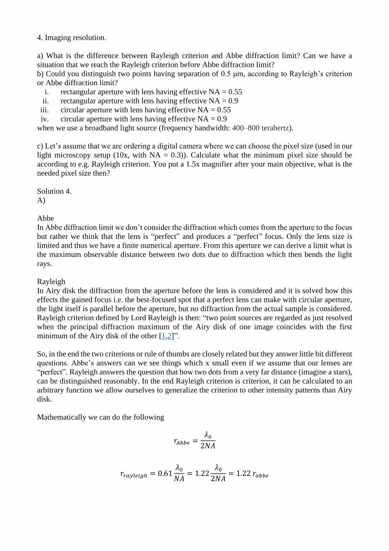
Mathematically we can do the following

𝑟𝐴𝑏𝑏𝑒 =𝜆0

2𝑁𝐴

𝑟𝑟𝑎𝑦𝑙𝑒𝑖𝑔ℎ = 0.61𝜆0

𝑁𝐴= 1.22

𝜆0

2𝑁𝐴= 1.22 𝑟𝑎𝑏𝑏𝑒

So mathematically speaking we can say that this is more restrictive and that it is a modification of

the abbe diffraction limit. I have though now assumed the following to hold

𝑟𝑟𝑎𝑦𝑙𝑒𝑖𝑔ℎ = 1.22𝜆0

2𝑁𝐴= 1.22

𝜆0

𝑁𝐴𝑜𝑏𝑗 + 𝑁𝐴𝑐𝑜𝑛𝑑

If this doesn’t hold, we can choose so small 𝑁𝐴𝑐𝑜𝑛𝑑 that Abbes diffraction limit is reached first.

B)

Following tables answers this question

Circl Rect

NA Rayleigh [µm]

Rayleigh [µm]

Abbe [µm]

0.55 0.62 2.0 0.51

0.9 0.38 1.2 0.31

𝛿𝑓 =

400𝑇ℎ𝑧,

d=0.5 μm

Rectangular

aperture

Circular

aperture

Abbe

diffraction

limit

NA=0.55 No No No

NA=0.90 No Yes Yes

I have used that �̅� =749 𝑛𝑚+375 𝑛𝑚

2= 562 𝑛𝑚

C)

With Rayleigh criterion minimum pixel size without any magnification

𝑟 = 0.61 𝜆

𝑁𝐴= 0.61

0.562 µ𝑚

0.3= 1.14 µ𝑚

So with 10x magnifier we have

𝑟10𝑥 = 𝑟 ∗ 10 = 11.4 µ𝑚

If we add 1.5x magnifier we have

𝑟15𝑥 = 𝑟10𝑥 ∗ 1.5 = 17.14 µ𝑚

So in pixels we want to have half of this value (one pixel for each object, one for each space

between) or rather having more than half of this value doesn’t really make the image better.

𝑟𝑝15𝑥 = 5.71 µ𝑚

𝑟𝑝15𝑥 = 8.57 µ𝑚

5. Aberrations in optical systems.

What is the definition of aberrations? Describe all the typical aberrations in optical systems (6 in

total). How one can compensate for the aberrations? How we can model the aberrations

mathematically and how we can distinguish aberrations from each other? How we can use this model

in practice to find out what aberrations there are in our optical system?

Solution 5.

Basically good sources of information is Hecht, Fundamentals of light microscopy and electronic

imaging, Lecture material (Lecture 3 “Bio-Imaging_MATR340_Autumn_2020_L_03.pdf”), and

Wikipedia although Wikipedia’s article is little bit outdated. There are of course lot of other material

in the internet which I haven’t mentioned.

Definition of aberration: departures or difference of the lens system, to the predicted outcome by the

Gaussian Optics. I.e. everything which doesn’t go as Gaussian optics predicts in the optical system

is an aberration.

To list different aberrations

Monochromatic (Seidel’s five aberrations)

• Spherical: Our lenses are spherical which isn’t the optimal shape→ Parallel rays (orthogonal

to the optical axis) which hit different locations (centre or the edge) focus to different spots.

→Fix add more lenses.

• Coma, off axis rays going through the centre of the lens or near the edge focus differently.

Coma is function of thin lens shape.

→Coma can be corrected by using a combination of lenses that are positioned symmetrically

around a central stop. In order to eliminate coma, the Abbe sine condition must be fulfilled

• Astigmatism: Occurs for objects (or parts of objects) away from the optical axis, happens even

for symmetrical lenses. Below a picture explaining the situation a little bit. Since we have

more surface in “y” direction than in “x” direction these directions have basically different

refractive indexes → Sagittal Plane and meridional planes have different focal points

The aberration is manifested by the off-axis image of a specimen point appearing as a line or

ellipse instead of a point

→ Corrected by adding lenses from microscopyU “Astigmatism errors are usually corrected

by design of the objectives to provide precise spacing of individual lens elements as well as

appropriate lens shapes, aperture sizes, and indices of refraction. The correction of

astigmatism is often accomplished in conjunction with the correction of field curvature

aberrations.”

• Field curvature (Petzval curvature): Focus plane isn’t a plane but a curve. Petzval surface in

inward towards the lens in positive and for negative lenses it curves outwards. If we fulfil

Petzval condition, the field is flat.

→ Suitable combination of negative and positive lenses will negate field curvature.

• Distortion: Transverse magnification may be a function of the off-axis image distance. So the

magnification can be different for different rays. In other words distortion arises because in

different are of the lens we have different focal length and different magnifications. Stops can

introduce distortion also (see picture below) so one must properly place them, thick simple

lenses generally suffer from distortion. Two different types, barrel (negative) and pincushion

(positive) (see picture below).

→ Proper design → no distortion, orthoscopic system.

• Chromatic aberrations

o Caused by dispersion, refractive index is function of wavelength.

→Different wavelengths have different focuses

→Fix add lenses.

Below is shown what Fundamentals of light microscopy and electronic imaging says about the

different aberration in a simple lens.

Chromatic aberration

“Chromatic aberration occurs because a lens refracts light differently, depending on the wavelength. Blue

light is bent inward toward the optical axis more than red light. The result is disastrous: Blue wavelengths

are focused in an image plane closer to the lens than the image plane for red wavelengths. Even at the best

focus, point sources are surrounded by colour halos, the colour changing depending on the focus of the

objective, the image never becoming sharp. Since each wavelength is focused at a different distance from

the lens, there is also a difference in magnification for different colours (chromatic magnification

difference). The solution is to make compound lenses made of glasses having different colour - dispersing

properties. For example, glass types known as crown and flint are paired together to make an achromatic

doublet lens that focuses blue and red wavelengths in the same image plane.”

Source: Fundamentals of light microscopy and electronic imaging

Spherical aberration

“Spherical aberration is the undesirable consequence of having lenses figured with spherical surfaces, the

only practical approach for lens manufacture. Parallel rays incident at central and peripheral locations on

the lens are focused at different axial locations, so that there is not a well - defined image plane, and a

point source of light at best focus appears as a spot surrounded by a bright halo or series of rings. For an

extended object, the entire image is blurred, especially at the periphery. One common solution is to use a

combination of positive and negative lenses of different thicknesses in a compound lens design.

Corrections for spherical aberration are made assuming a certain set of conditions: coverslip thickness,

the assumption that the focal plane is at or near the coverslip surface, the refractive index of the medium

between lens and coverslip, the wavelength of illumination, temperature, and others. Thus, users

employing well - corrected objectives can unknowingly induce spherical aberration by using coverslips

having the wrong thickness, by warming the objective, or by focusing on objects positioned away from

the coverslip surface. Special objectives are now available with adjustable correction collars to minimize

spherical aberration (Brenner, 1994).”

Source: Fundamentals of light microscopy and electronic imaging

Coma

“Coma is an “off - axis aberration” that causes point objects to look like comets, focused spots with

emanating comet tails, located at the periphery of an image. Coma affects the images of points located off

the optical axis — that is, when object rays hit the lens obliquely. It is the most prominent off - axis

aberration. Rays passing through the edge of the lens are focused farther away from the optical axis than

are rays that pass through the center of the lens, causing a point object to look like a comet with the tail

extending toward the periphery of the fi eld. Coma is greater for lenses with wider apertures. Correction

for this aberration is made to accommodate the diameter of the object fi eld for a given objective.”

Source: Fundamentals of light microscopy and electronic imaging

Astigmatism

“Astigmatism, like coma, is an off - axis aberration. Rays from an object point passing through the

horizontal and vertical diameters of a lens are focused as a short streak at two different focal planes. The

streaks appear as ellipses drawn out in horizontal and vertical directions at either side of best focus, where

the focused image of a point appears as an extended circular patch. Off - axis astigmatism increases with

increasing displacement of the object from the optical axis. Astigmatism is also caused by asymmetric

lens curvature due to mistakes in manufacture or improper mounting of a lens in its barrel.”

Source: Fundamentals of light microscopy and electronic imaging

Curvature of field

“Curvature of field is another serious off - axis aberration. Field curvature indicates that the image plane

is not flat, but has the shape of a concave spherical surface as seen from the objective. Different zones of

the image can be brought into focus, but the whole image cannot be focused simultaneously on a flat

surface as would be required for photography. Field curvature is corrected by the lens design of the

objective and additionally by the tube or relay lens and sometimes the oculars.”

Source: Fundamentals of light microscopy and electronic imaging

Distortion of field

“Distortion is an aberration that causes the focus position of the object image to shift laterally in the image

plane with increasing displacement of the object from the optical axis. The consequence of distortion is a

nonlinear magnifi cation in the image from the center to the periphery of the field. Depending on whether

the gradient in magnification is increasing or decreasing, the aberration is termed pincushion or barrel

distortion after the distorted appearance of a specimen with straight lines, such as a grid or reticule with a

pattern of squares or rectangles. Corrections are made as described for field curvature.”

Source: Fundamentals of light microscopy and electronic imaging