lab09wsolns

* Notes based on Chapters 9 and 11 from Applied Numerical Methods with MATLAB for Engineers and Scientists, Steven C. Chapra, 3rd Edition, McGraw-Hill, 2012.

Lab #9: Systems of Linear Equations*

1 Methods for solving systems of linear equations 1.1 Matrix Inversion (Lab #8)

1.2 Substitution

Example: For the system

Substitute 2nd equation into 1st:

Solve for :

Substitute into one of the original equations and solve for :

1.3 Graphical Method (up to 3 variables) Example: For the system

Plot all equations:

Point at which all lines intersect is the solution:

This technique helps find out problems with the system:

1.4 Cramer’s Rule For a system expressed as , where:

We can solve for the unknowns by taking the ratio:

where and is the determinant of the matrix obtained by replacing column ( ) with . Example: For the system

The system of equations is expressed as:

and and are:

1.5 Gauss Elimination

Sequential process of removing unknowns using “forward elimination” and “back substitution”. For a system in the form , express as:

1.5.1 Forward Elimination

For each row, subtract multiples of previous rows to eliminate coefficients until you get an upper triangular matrix. i. Eliminate from row 2:

where:

Now the matrix looks like:

ii. Eliminate from row 3:

where:


iii. Eliminate

from row 3:

where:


equation with only one unknown

1.5.2 Back Substitution

Transform matrix back to equations:

Solve 3rd equation for :

Solve 2nd equation for :

Solve 1st equation for :

Coding Gauss Elimination from numpy import size,append,zeros

from sys import exit

def GaussNaive(A,B):

# GaussNaive: Naive Gauss Elimination

# X = GaussNaive(A,B): Gauss elimination without pivoting.

# input:

# A = coefficient matrix

# B = constant matrix

# output:

# X = solution vector

# Check that coefficient matrix is square

m = size(A,0)

n = size(A,1)

if m != n:

print '\nMatrix A must be square.\n'

exit(0)

# Concatenate A and B

Aug = append(A,B,1)

nB = n+1

# Forward elimination

for k in range(0,n-1):

for i in range(k+1,n):

factor = Aug[i,k]/Aug[k,k]

for j in range(k,nB):

Aug[i,j] = Aug[i,j]-factor*Aug[k,j]

# Back substitution

X = zeros((n,1))

X[n-1] = Aug[n-1,n]/Aug[n-1,n-1]

for i in range(n-2,-1,-1):

X[i] = Aug[i,n]

for j in range(i+1,n):

X[i] = X[i]-Aug[i,j]*X[j]

X[i] = X[i]/Aug[i,i]

# Return solution

return X

Example: Use Gauss Elimination to solve:

Generate the coefficient matrix , and vector , and feed to the GaussNaive function shown above: from GaussNaive import GaussNaive

from numpy import array

# For same problem that we solved with other methods:

# 2x + 3y = 14

# -4x + y = 28

A = array([[2.,3.],[-4.,1.]])

B = array([[14.],[28.]])

X = GaussNaive(A,B)

print X

The output is: [[-5.]

[ 8.]]

1.5.3 Pivoting

What happens if a coefficient along the diagonal of the matrix is zero? Example: Solve

In matrix form:

Zeros in the diagonal will cause division by zero in the forward elimination step.

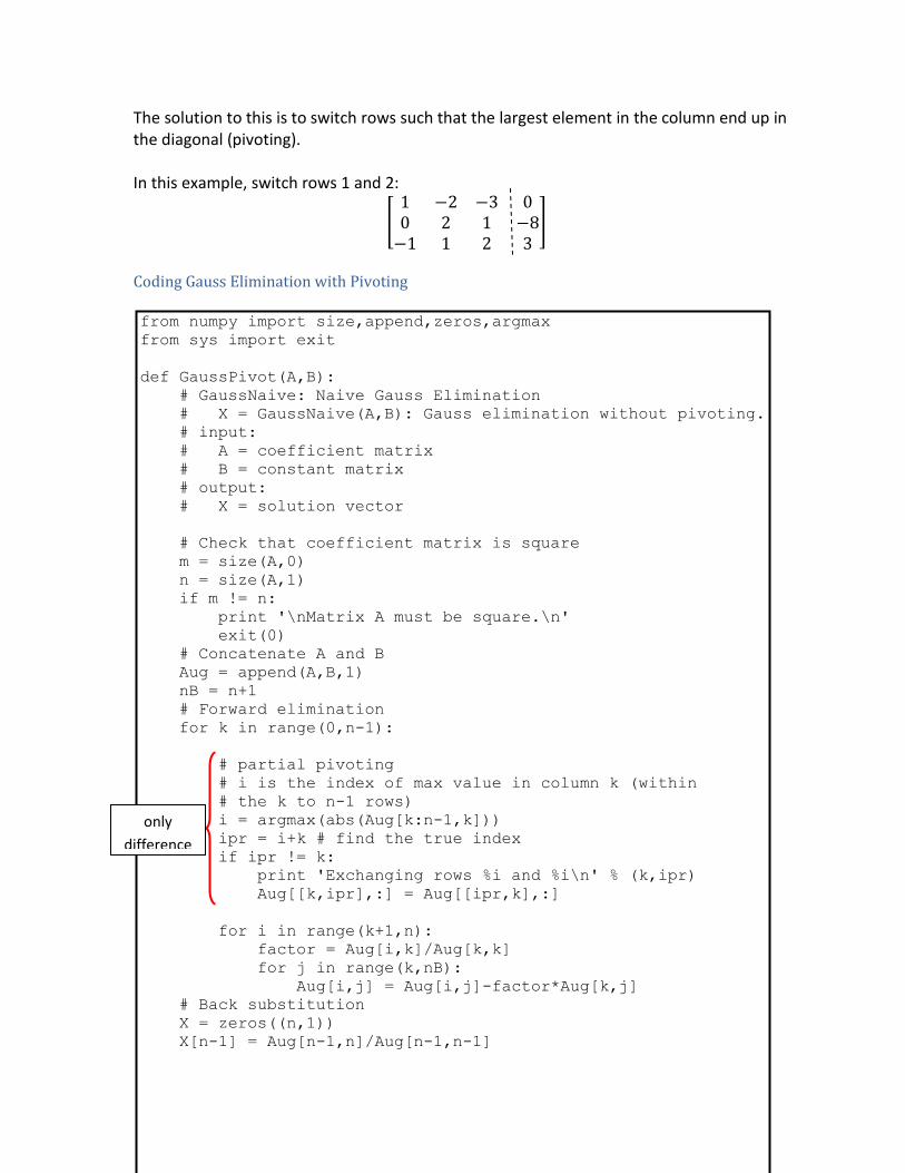
The solution to this is to switch rows such that the largest element in the column end up in the diagonal (pivoting). In this example, switch rows 1 and 2:

Coding Gauss Elimination with Pivoting from numpy import size,append,zeros,argmax

from sys import exit

def GaussPivot(A,B):

# GaussNaive: Naive Gauss Elimination

# X = GaussNaive(A,B): Gauss elimination without pivoting.

# input:

# A = coefficient matrix

# B = constant matrix

# output:

# X = solution vector

# Check that coefficient matrix is square

m = size(A,0)

n = size(A,1)

if m != n:

print '\nMatrix A must be square.\n'

exit(0)

# Concatenate A and B

Aug = append(A,B,1)

nB = n+1

# Forward elimination

for k in range(0,n-1):

# partial pivoting

# i is the index of max value in column k (within

# the k to n-1 rows)

i = argmax(abs(Aug[k:n-1,k]))

ipr = i+k # find the true index

if ipr != k:

print 'Exchanging rows %i and %i\n' % (k,ipr)

Aug[[k,ipr],:] = Aug[[ipr,k],:]

for i in range(k+1,n):

factor = Aug[i,k]/Aug[k,k]

for j in range(k,nB):

Aug[i,j] = Aug[i,j]-factor*Aug[k,j]

# Back substitution

X = zeros((n,1))

X[n-1] = Aug[n-1,n]/Aug[n-1,n-1]

only

difference

for i in range(n-2,-1,-1):

X[i] = Aug[i,n]

for j in range(i+1,n):

X[i] = X[i]-Aug[i,j]*X[j]

X[i] = X[i]/Aug[i,i]

# Return solution

return X

Solve example problem using this code:

from GaussNaive import GaussNaive

from GaussPivot import GaussPivot

from numpy import array

# Problem for Gauss elimination with pivoting:

# 2y + z = -8

# x - 2y - 3z = 0

# -x + y + 2z = 3

A = array([[0.,2.,1.],[1.,-2.,-3.],[-1.,1.,2.]])

B = array([[-8.],[0.],[3.]])

XN = GaussNaive(A,B)

XP = GaussPivot(A,B)

print 'X_naive:'

print XN

print 'X_pivot:'

print XP

x = XP[0]

y = XP[1]

z = XP[2]

print 'vector B:'

print 2.*y+z, x-2.*y-3.*z, -x+y+2.*z

The output from this script is: Exchanging rows 0 and 1

X_naive:

[[ nan]

[ nan]

[ nan]]

X_pivot:

[[-4.]

[-5.]

[ 2.]]

vector B:

[-8.] [ 0.] [ 3.]

1.6 Example: Model of a Heated Rod For a long thin rod positioned between two walls that are held at constant temperature, the steady-state energy conservation equation is written as:

where = temperature (°C), = distance along the rod (m), = a heat transfer coefficient between the rod and the surrounding air (m-2), and = air temperature (°C).

This equation can be solved analytically to give:

when = 0.01, = 20, = 40 and = 200. But another way of solving it, is by using finite differences to transform the differential equation into a system of linear algebraic equations, and use any of the methods described so far to solve for the unknowns. Step 1: Divide the rod into a series of discrete segments separated by nodes for which we will find the temperature. As seen in the figure, the tube has a total length of 10 m, and we will divide it into five segments, each with a length = 10/5 = 2 m. This discretization defines six nodes (0 to 5) at the boundaries between the different segments. Step 2: Substitute derivatives in the original equation by finite difference approximations. Note: Remember from Lab #4,

Substituting the finite difference approximation for the second derivative in the equation gives:

And rearranging gives:

Step 3: Apply the resulting equation to each of the interior nodes:

= 0.01*22+2 = 2.04 = 0.01*22*20 = 0.8 For node 1: For node 2: For node 3: For node 4:

Substitute the values for and , which we already know:

For node 1: For node 2: For node 3: For node 4:

Step 4: Solve the system of linear algebraic equations: from numpy import matrix,arange,exp,append

from numpy.linalg import inv

from pylab import figure,plot,xlabel,ylabel,legend

h = 0.01 # in m^(-2)

Ta = 20. # in C

L = 10. # in m

N = 6 # number of nodes

T0 = 40. # in C

T5 = 200. # in C

dx = L/(N-1)

q1 = h*dx*dx+2.

q2 = h*dx*dx*Ta

A = matrix([[ q1,-1., 0., 0.],

[-1., q1,-1., 0.],

[ 0.,-1., q1,-1.],

[ 0., 0.,-1., q1]])

B = matrix([[q2+T0],

[q2],

[q2],

[q2+T5]])

T = inv(A)*B

T = append(T0,T)

T = append(T,T5)

x = arange(0.,L+1.,dx)

T_exact = 73.4523*exp(0.1*x)-53.4523*exp(-0.1*x)+20.

figure()

plot(x,T,'p',x,T_exact)

xlabel('distance along the rod (m)')

ylabel('Temperature (C)')

legend(('approximation', 'exact soln.'), loc='upper left')

And the output is:

2. Matrix Inverse and Condition 2.1 Response and Stimulus

For systems that can be expressed as:

or

response stimulus connects

stimulus to

response

Example: If you want to know how affects , you look at .

This also works with changes.

Example: If you want to know how a change in changes :

2.2 Ill-conditioned systems

Three ways in which we can use the coefficient matrix to identify an ill-conditioned system:

- Scale such that largest element in each row has a value of 1. If any , then the system

is ill-conditioned. - If , then the system is ill-conditioned. - If , then the system is ill-conditioned.

2.3 Example: Indoor Air Pollution

Analyze the ventilation system for a restaurant near a freeway.

Step 1 Write steady-state mass balances for each room and solve the resulting linear algebraic equations for the concentration of carbon monoxide in each room. To arrive at the mass balances for the different rooms, one needs to consider that in the figure, the one-way arrows represent volumetric flows, while the two-way arrows represent diffusive mixing only. This means that we need to solve for the flows occurring between rooms ( , and ). A balance on room 1 gives:

a balance on room 3 gives:

and a balance on room 4 gives:

Note that, in my equation, I assumed that was going from room 2 to room 4, but the value turned out to be negative, so is actually going from room 4 into room 2 ( ). Now that we know all the flows, we can solve for the mass balances. For room 1:

For room 2:

For room 3:

For room 4:

Express these four balances in matrix form:

Enter into a script and solve for through : from numpy import matrix


# Enter data

ca = 2. # mg/m3

cb = 2. # mg/m3

Qa = 200. # m3/hr

Qb = 50. # m3/hr

Qc = 150. # m3/hr

Qd = 100. # m3/hr

E13 = 25. # m3/hr

E24 = 25. # m3/hr

E34 = 50. # m3/hr

Wsmoker = 1000. # mg/hr

Wgrill = 2000. # mg/hr

# Setup coefficient matrix and stimuli vector

A = matrix([[Qa+E13 ,0. ,-E13 ,0. ],

[0. ,Qc+E24,0. ,-Qa+Qd-E24],

[-Qa-E13,0. ,Qa+E13+E34,-E34 ],

[0. ,-E24 ,-Qa-E34 ,Qa+E34+E24]])

B = matrix([[Wsmoker+Qa*ca],

[Qb*cb ],

[Wgrill ],

[0. ]])

# Solve for concentrations

C = inv(A)*B

print C

The output is: [[ 8.09961686]

[ 12.34482759]

[ 16.89655172]

[ 16.48275862]]

Step 2 Generate the matrix inverse and use it to analyze how the various sources affect the kid’s room. For example, determine what percent of the carbon monoxide in the kid’s section is due to (1) the smokers, (2) the grill and (3) the intake vents. In addition, compute the improvement in the kid’s section concentration if the carbon monoxide load is decreased by banning smoking and fixing the grill. Once we have the inverse of the coefficient matrix, we can express the solution as:

Where the coefficients of the inverse of give us the relationship between the stimuli (forcing function) and the solution (response). To get the concentration of carbon monoxide in the kids’ section ( ) due to the smokers ( ), we look at

:

To get the concentration of carbon monoxide in the kids’ section ( ) due to the grill ( ), we look at

:

To get the concentration of carbon monoxide in the kids’ section ( ) due to the intakes (

), we look at and

:

In addition, because the model is linear, superposition holds and the impact of banning smoking and fixing the grill can be determined individually and summed:

Adding this calculation to the script results in: from numpy import matrix


# Enter data

ca = 2 # mg/m3

cb = 2 # mg/m3

Qa = 200 # m3/hr

Qb = 50 # m3/hr

Qc = 150 # m3/hr

Qd = 100 # m3/hr

E13 = 25 # m3/hr

E24 = 25 # m3/hr

E34 = 50 # m3/hr

Wsmoker = 1000 # mg/hr

Wgrill = 2000 # mg/hr


A = matrix([[Qa+E13 ,0. ,-E13 ,0. ],

[0. ,Qc+E24,0. ,-Qa+Qd-E24],

[-Qa-E13,0. ,Qa+E13+E34,-E34 ],

[0. ,-E24 ,-Qa-E34 ,Qa+E34+E24]])


[Qb*cb ],

[Wgrill ],

[0. ]])


C = inv(A)*B

# Take the inverse of the coefficient matrix

Ainv = inv(A)

# Contributions from smokers, grill and intakes to kid's section

per_smokers = Ainv[1,0]*Wsmoker/C[1]*100.

print 'per_smokers = ',per_smokers

per_grill = Ainv[1,2]*Wgrill/C[1]*100.

print 'per_grill = ',per_grill

per_intakes = (Ainv[1,0]*Qa*ca+Ainv[1,1]*Qb*cb)/C[1]*100.

print 'per_intakes = ',per_intakes

# Change in kid's section due to banning smoking and fixing the

grill

dC2 = -Ainv[1,0]*Wsmoker-Ainv[1,2]*Wgrill

print 'dC2 = ',dC2

C2_new = C[1]+dC2

print 'C2_new = ',C2_new

The output from this script is: per_smokers = [[ 27.93296089]]

per_grill = [[ 55.86592179]]

per_intakes = [[ 16.20111732]]

dC2 = -10.3448275862

C2_new = [[ 2.]]

Step 3 Analyze how the concentration in the kid’s area would change if a screen is constructed so that the mixing between areas 2 and 4 is decreased to 5 m3/hr. This change involves changing the value for from 25 to 5 m3/hr, which is one of the inputs for the coefficient matrix. It makes things clearer and cleaner if we now generate the coefficient matrix in a separate function: from numpy import matrix

def ventilation(Qa,E13,Qc,E24,Qd,E34,Wsmoker,ca,Qb,cb,Wgrill):

A = matrix([[Qa+E13,0.,-E13,0.],

[0.,Qc+E24,0.,-Qa+Qd-E24],

[-Qa-E13,0.,Qa+E13+E34,-E34],

[0.,-E24,-Qa-E34,Qa+E34+E24]])


[Qb*cb],

[Wgrill],

[0.]])

return A,B

This makes it easier to regenerate the coefficient matrix everytime we change the input. The script for this section looks now like: from numpy.linalg import inv

from ventilation import ventilation

# Enter data

ca = 2 # mg/m3

cb = 2 # mg/m3

Qa = 200 # m3/hr

Qb = 50 # m3/hr

Qc = 150 # m3/hr

Qd = 100 # m3/hr

E13 = 25 # m3/hr

E24 = 25 # m3/hr

E34 = 50 # m3/hr

Wsmoker = 1000 # mg/hr

Wgrill = 2000 # mg/hr


[A,B] = ventilation(Qa,E13,Qc,E24,Qd,E34,Wsmoker,ca,Qb,cb,Wgrill)


C1 = inv(A)*B

# Install screen

E24 = 5 # m3/hr

# Setup new coefficient matrix and stimuli vector

[A,B] = ventilation(Qa,E13,Qc,E24,Qd,E34,Wsmoker,ca,Qb,cb,Wgrill)

# Solve for new concentrations

C2 = inv(A)*B

# Take the difference in the kid's section concentration

dC2 = C2[1]-C1[1]

print 'dC2 = ',dC2

dC2 = [[-0.26482759]]

The decrease in the concentration of carbon monoxide in the kids’ section due to installation of the screen is 0.2648 mg/m3.

3. Practice Problems Problem 1:

A furnace wall is made up of three separate materials. Let represent the thermal conductivity of material , let represent the corresponding thickness ( ), and let and represent the convective heat transfer coefficients of the outer surfaces. If , then the following steady-state heat transfer equations apply:

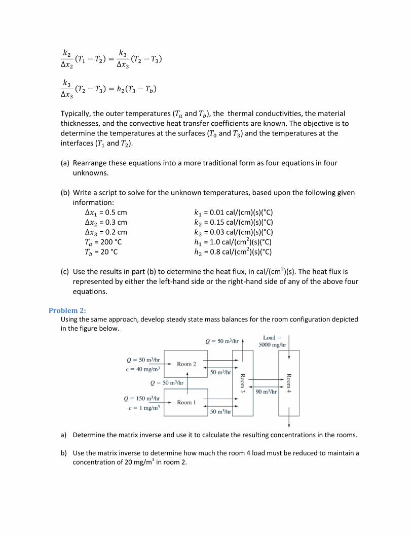
Typically, the outer temperatures ( and ), the thermal conductivities, the material thicknesses, and the convective heat transfer coefficients are known. The objective is to determine the temperatures at the surfaces ( and ) and the temperatures at the interfaces ( and ). (a) Rearrange these equations into a more traditional form as four equations in four

unknowns.

(b) Write a script to solve for the unknown temperatures, based upon the following given information:

= 0.5 cm = 0.01 cal/(cm)(s)(°C) = 0.3 cm = 0.15 cal/(cm)(s)(°C) = 0.2 cm = 0.03 cal/(cm)(s)(°C) = 200 °C = 1.0 cal/(cm2)(s)(°C) = 20 °C = 0.8 cal/(cm2)(s)(°C)

(c) Use the results in part (b) to determine the heat flux, in cal/(cm2)(s). The heat flux is represented by either the left-hand side or the right-hand side of any of the above four equations.

Problem 2: Using the same approach, develop steady state mass balances for the room configuration depicted in the figure below.

a) Determine the matrix inverse and use it to calculate the resulting concentrations in the rooms.

b) Use the matrix inverse to determine how much the room 4 load must be reduced to maintain a

concentration of 20 mg/m3 in room 2.

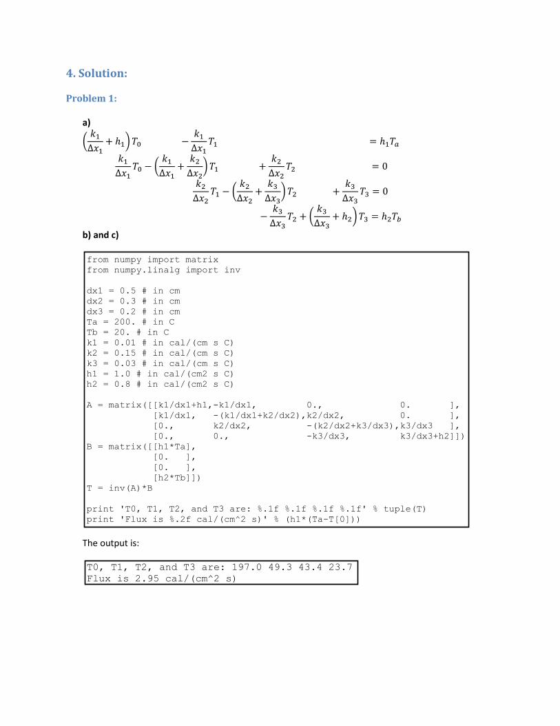
4. Solution: Problem 1:

a)

b) and c)

from numpy import matrix


dx1 = 0.5 # in cm

dx2 = 0.3 # in cm

dx3 = 0.2 # in cm

Ta = 200. # in C

Tb = 20. # in C

k1 = 0.01 # in cal/(cm s C)

k2 = 0.15 # in cal/(cm s C)

k3 = 0.03 # in cal/(cm s C)

h1 = 1.0 # in cal/(cm2 s C)

h2 = 0.8 # in cal/(cm2 s C)

A = matrix([[k1/dx1+h1,-k1/dx1, 0., 0. ],

[k1/dx1, -(k1/dx1+k2/dx2),k2/dx2, 0. ],

[0., k2/dx2, -(k2/dx2+k3/dx3),k3/dx3 ],

[0., 0., -k3/dx3, k3/dx3+h2]])

B = matrix([[h1*Ta],

[0. ],

[0. ],

[h2*Tb]])

T = inv(A)*B

print 'T0, T1, T2, and T3 are: %.1f %.1f %.1f %.1f' % tuple(T)

print 'Flux is %.2f cal/(cm^2 s)' % (h1*(Ta-T[0]))

The output is: T0, T1, T2, and T3 are: 197.0 49.3 43.4 23.7

Flux is 2.95 cal/(cm^2 s)

Problem 2: Flow balances can be used to compute:

Also, let us identify the different loads on each of the rooms:

load on Room 1

load on Room 2

load on Room 4

Then the steady-state mass balances can be written for the rooms as

Our matrix system looks like:

The concentration in Room 2 as a function of the change in load to the Room 4 can be formulated in terms of the matrix inverse as

which can be solved for

The matrix system is saved as a function: from numpy import matrix

def ventilation2(Q12,Q13,E13,Q23,E23,Q34,Q3out,E34,Q4out,W1,W2,W4):

A = matrix([[Q12+Q13+E13,0.,-E13,0.],

[-Q12,Q23+E23,-E23,0.],

[-Q13-E13,-Q23-E23,Q34+Q3out+E13+E23+E34,-E34],

[0.,0.,-Q34-E34,Q4out+E34]])

B = matrix([[W1],

[W2],

[0.],

[W4]])

return A,B

Then the main script is written to call the function with the matrix to solve for the unknowns: from ventilation2 import ventilation2

from numpy import transpose


# Enter data

Q12 = 50. # m3/hr

Q13 = 100. # m3/hr

Q23 = 100. # m3/hr

Q34 = 150. # m3/hr

Q3out = 50. # m3/hr

Q4out = 150. # m3/hr

E13 = 50. # m3/hr

E23 = 50. # m3/hr

E34 = 90. # m3/hr

W1 = 150. # mg/hr

W2 = 2000. # mg/hr

W4 = 5000. # mg/hr


[A,B] =

ventilation2(Q12,Q13,E13,Q23,E23,Q34,Q3out,E34,Q4out,W1,W2,W4)


C = inv(A)*B

print 'concentrations are: ', transpose(C)

# Calculate resuction in room 4 load to get C2 to 20mg/m3

Ainv = inv(A)

delta_W4 = (20.-C[1])/Ainv[1,3]

print 'delta_W4 = ',delta_W4

The results are: concentrations are: [[ 5.78125 21.96875 20.125

40.95833333]]

delta_W4 = [[-2520.]]

lab09wsolns

Documents