lab testing user guide · fall head k and fhk readings falling head permeability testing data....
TRANSCRIPT

Lab Testing User Guide gINT V8i User Manual
DAA039510-1/0001

— 1 —
The information in this publication is subject to change without notice and does not represent a commitment on the part of Bentley. The software described in this document is furnished under a license agreement or nondisclosure agreement. The software must be used or copied only in accordance with the terms of the agreement.
COPYRIGHT NOTICE
Copyright (c) 2011 Bentley Systems, Incorporated. All rights reserved.
Including software, file formats, and audiovisual displays; may only be used pursuant to applicable software license agreement; contains confidential and proprietary information of Bentley Systems, Incorporated and/or third parties which is protected by copyright and trade secret law and may not be provided or otherwise made available without proper authorization.
RESTRICTED RIGHTS LEGENDS
If this software is acquired for or on behalf of the United States of America, its agencies and/or instrumentalities ("U.S. Government"), it is provided with restricted rights. This software and accompanying documentation are "commercial computer software" and "commercial computer software documentation," respectively, pursuant to 48 C.F.R. 12.212 and 227.7202, and "restricted computer software" pursuant to 48 C.F.R. 52.227-19(a), as applicable. Use, modification, reproduction, release, performance, display or disclosure of this software and accompanying documentation by the U.S. Government are subject to restrictions as set forth in this Agreement and pursuant to 48 C.F.R. 12.212, 52.227-19, 227.7202, and 1852.227-86, as applicable. Contractor/Manufacturer is Bentley Systems, Incorporated, 685 Stockton Drive, Exton, PA 19341-0678.
Unpublished - rights reserved under the Copyright Laws of the United States and International treaties.”
Bentley Systems Inc. Corporate Headquarters 685 Stockton Drive Exton, PA 19341, United States Web Site: http://www.bentley.com/en-US/Products/gINT/ Sales and General Support: http://www.bentley.com/en-US/Corporate/Contact+Us/

— 2 —
Contents Introduction ............................................................................................................................................ 5 Setting up Lab Testing ......................................................................................................................... 6
Adding Lab Testing Support .................................................................................................................. 6
Modifications Made when You Add Lab Testing Support ............................................................. 6
Removing Lab Testing Support ............................................................................................................ 8
Appending Items from the Most Recent Lab Testing Version .................................................. 9
Using Defaults and Calibrations ......................................................................................................... 10
Field Defaults ................................................................................................................................................ 10
Lab Testing User Interface ............................................................................................................... 12 Relational Database Structure ....................................................................................................... 13 Lab Testing Tables .............................................................................................................................. 15
Defining a Lab Specimen ....................................................................................................................... 15
LAB SPECIMEN table ................................................................................................................................. 15
Some Typical Reports ................................................................................................................................ 16
Water Content / Density ....................................................................................................................... 17
Background ................................................................................................................................................... 17
Data Entry ...................................................................................................................................................... 17
WC DENSITY table fields ......................................................................................................................... 18
Data Entry Scenarios and Calculations ............................................................................................. 19
Void Ratio and Saturation Calculations............................................................................................ 21
Some Typical Reports ................................................................................................................................ 23
Atterberg Analysis ................................................................................................................................... 26
Background ................................................................................................................................................... 26
Data Entry ...................................................................................................................................................... 27
ATTERBERG table fields ........................................................................................................................... 28
ATTB READINGS table fields .................................................................................................................. 29
Data Entry Scenarios and Calculations ............................................................................................. 30
Some Typical Reports ................................................................................................................................ 31
Sieve Analysis ............................................................................................................................................ 36
Background ................................................................................................................................................... 36
Data Entry ...................................................................................................................................................... 36 SIEVE table fields ........................................................................................................................................ 37
SV READINGS table fields ........................................................................................................................ 40

— 3 —
Data Entry Scenarios and Calculations ............................................................................................. 41
Setting up a Sieve Readings List in DATA DESIGN ....................................................................... 46
Setting up Individual Tares for Sieves ............................................................................................... 48
Some Typical Reports ................................................................................................................................ 49
Hydrometer Analysis .............................................................................................................................. 54 Background ................................................................................................................................................... 54
Data Entry ...................................................................................................................................................... 54
HYDROMETER table fields ...................................................................................................................... 55
HYD READINGS table fields .................................................................................................................... 56
Setting up Hydrometer Calibrations in the Library Table ........................................................ 58
Data Entry Scenarios and Calculations ............................................................................................. 62
Some Typical Reports ................................................................................................................................ 64
Fine Specific Gravity ................................................................................................................................ 65
Background ................................................................................................................................................... 65
Data Entry ...................................................................................................................................................... 65
FINE SG table fields .................................................................................................................................... 65
FINE SG READINGS table fields ............................................................................................................. 66
Data Entry Scenarios and Calculations ............................................................................................. 67
Some Typical Reports ................................................................................................................................ 67
Compaction ................................................................................................................................................. 68
Background ................................................................................................................................................... 68
Data Entry ...................................................................................................................................................... 68
COMPACTION table fields ........................................................................................................................ 69
COMP READINGS table fields ................................................................................................................. 71
Data Entry Scenarios and Calculations ............................................................................................. 72
Optional Calculation of Maximum Dry Density and Optimum Moisture Content ........... 74
Some Typical Reports ................................................................................................................................ 76
Unconfined Compression ...................................................................................................................... 80
Background ................................................................................................................................................... 80 Data Entry ...................................................................................................................................................... 81
UNCONF COMPR table fields .................................................................................................................. 82
UNC READINGS table fields .................................................................................................................... 84
Setting up Load Ring Calibrations in the Library Table ............................................................ 84
Data Entry Scenarios and Calculations ............................................................................................. 87
— 4 —
Some Typical Reports ................................................................................................................................ 91
Consolidation ............................................................................................................................................. 93
Background ................................................................................................................................................... 93
Data Entry ...................................................................................................................................................... 94
CONSOLIDATION table fields ................................................................................................................. 96 CONSOL READINGS table fields ............................................................................................................ 97
Data Entry Scenarios and Calculations ............................................................................................. 98
Some Typical Reports ............................................................................................................................. 100
Direct Shear ............................................................................................................................................. 103
Background ................................................................................................................................................ 103
Data Entry ................................................................................................................................................... 103
DIRECT SHEAR table fields .................................................................................................................. 105
DSHR READINGS table fields .............................................................................................................. 107
Data Entry Scenarios and Calculations .......................................................................................... 108
Reporting ..................................................................................................................................................... 108
Falling Head Permeability ................................................................................................................. 109
Background ................................................................................................................................................ 109
Data Entry ................................................................................................................................................... 110
FALL HEAD K table fields ..................................................................................................................... 111
FHK READINGS table fields ................................................................................................................. 115
Data Entry Scenarios and Calculations .......................................................................................... 116
Reporting ..................................................................................................................................................... 119
Appendix A -- Suggested Field Defaults .................................................................................... 120 Appendix B -- Lab Database Structure Manipulation .......................................................... 122
Adding Tables to Lab Testing Support .......................................................................................... 122
Parent is LAB SPECIMEN, relationship is one-to-one ............................................................... 122
Parent is LAB SPECIMEN, relationship is one-to-many ........................................................... 123
Making LAB SPECIMEN a Child of a Non-POINT Table .......................................................... 124
Extending the Keysets of Lab Testing Tables ............................................................................. 125
Appendix C -- Scenarios using Wet Specimens in Sieve Analysis .................................... 127 Scenario 5: Wet specimen, no split, incremental weighing .................................................. 127
Scenario 6: Wet specimen, split sieve ........................................................................................... 128
Scenario 7: Wet specimen, coarse fraction sieved wet .. Error! Bookmark not defined.
— 5 —
Introduction
The lab testing subsystem of gINT is a suite of laboratory test tables that integrate with each other and with other areas of gINT. Using the gINT lab testing module, you can automate the calculation of all the computed values you normally generate from your raw lab data, and report on a wide range of lab data in combination with borehole data.
This user guide provides in-depth reference information for understanding the lab testing tables and fields, their purposes, their interdependencies, and how data is reported. The user guide can be read from start to finish, or referenced for information on specific topics. To learn about lab testing without reading the entire user guide, and with step-by-step hands-on examples, we recommend the gINT tutorial entitled Using gINT Lab Testing, or the gINT University course gINT 007 - Lab Testing.
This user guide is divided into chapters by test (each corresponding to one tab in the Lab Testing tab bar). Also, an introductory chapter is provided at the beginning of the user guide, describing how lab testing is set up for the first time. In each test-specific chapter, the following sections are provided:
• Background: Briefly describes what the test is for and how it is performed • Data entry: Overview of how data entry is performed, and the field
interdependencies • Field descriptions: Details on each field in the table or tables maintained in the tab • Data entry scenarios: Example data for various scenarios • Reporting: Descriptions of reports that utilize the test’s data • Special topics: Included if any are relevant
Note that the “Background” sections rely heavily on information from Soil Testing Manual: Procedures, Classification Data, and Sampling Practices, by Robert W. Day (McGraw Hill, 2001). Where this reference book has been quoted directly, page number references are provided.

— 6 —
Setting up Lab Testing
Adding Lab Testing Support
To add lab testing support to a database that lacks it (either a project or data template file), go to INPUT and open the database. Under the Additional Modules menu you will see Lab Testing Support. If this has a checkmark, then lab testing support is already in the database, otherwise select that menu item. [Alternately you can add lab testing support in DATA DESIGN.]
If you add lab testing support to a data template file (or generate the template from a project that has lab testing), then you can clone this file to create new projects. The lab testing tables will be cloned with the non-lab tables, eliminating the need to add lab testing support to each project. We recommend this approach.
Most of the fields supplied by the program when lab testing support is added cannot be deleted and only their Default, Description, and Caption properties can be modified. Other fields are optional and can be deleted or modified like any other field you would add. You can add your own fields to any of the lab testing tables and you can rearrange the order of the fields for data entry.
Modifications Made when You Add Lab Testing Support
Database Tables Added
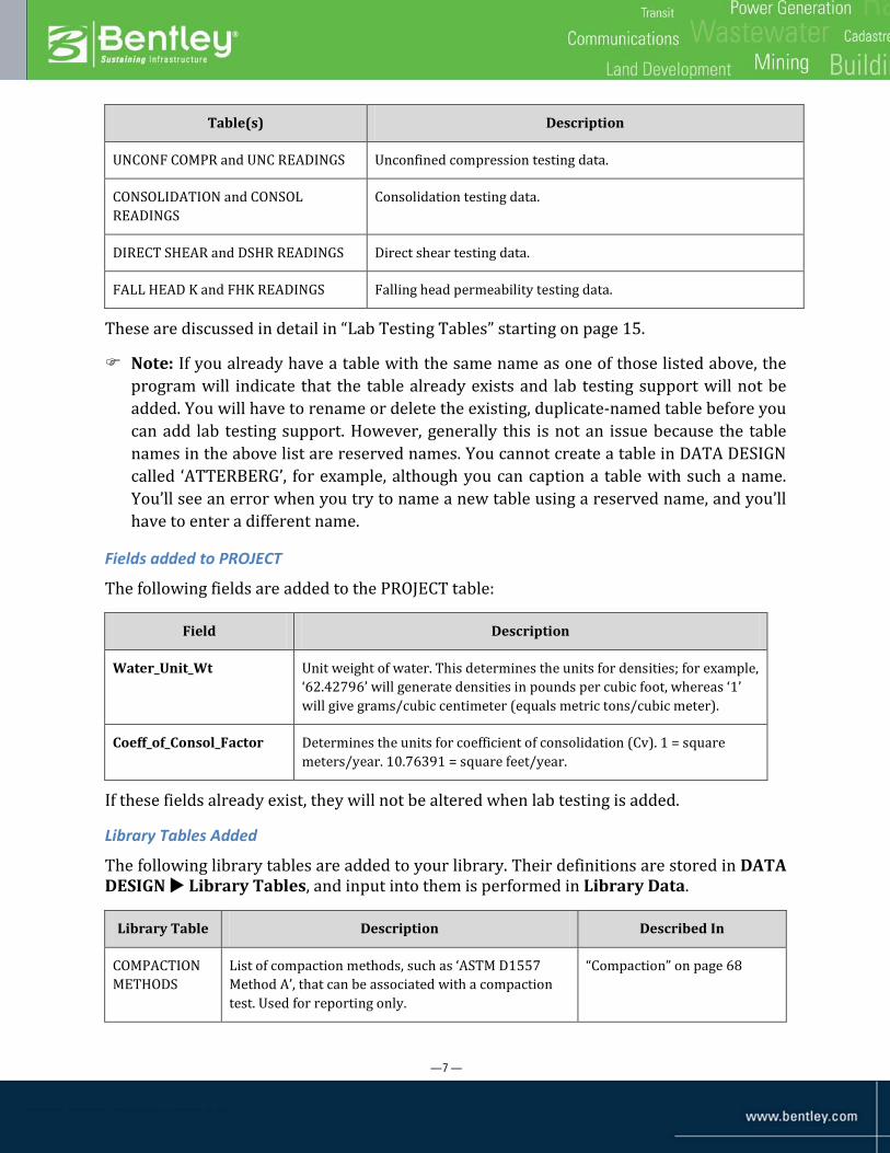
The following tables are added to the database when you add lab testing support:
Table(s) Description
LAB SPECIMEN This is the parent table of all lab testing tables. Each test specimen is identified by a unique PointID-Depth combination. Optional data can also be entered that relates to the specimen, such as color and consistency.
WC DENSITY Water content, wet density, and dry density data for the specimen.
ATTERBERG and ATTB READINGS Liquid and plastic limits computed from Casagrande or cone penetrometer techniques.
SIEVE and SV READINGS Grain size distribution using sieve analysis.
HYDROMETER and HYD READINGS Grain size distribution of fine particles using hydrometer analysis.
FINE SG and FINE SG READINGS Fine (less than #4 sieve) particles specific gravity data.
COMPACTION and COMP READINGS Compaction testing data.
— 7 —
Table(s) Description
UNCONF COMPR and UNC READINGS Unconfined compression testing data.
CONSOLIDATION and CONSOL READINGS
Consolidation testing data.
DIRECT SHEAR and DSHR READINGS Direct shear testing data.
FALL HEAD K and FHK READINGS Falling head permeability testing data.
These are discussed in detail in “Lab Testing Tables” starting on page 15.
Note: If you already have a table with the same name as one of those listed above, the program will indicate that the table already exists and lab testing support will not be added. You will have to rename or delete the existing, duplicate-named table before you can add lab testing support. However, generally this is not an issue because the table names in the above list are reserved names. You cannot create a table in DATA DESIGN called ‘ATTERBERG’, for example, although you can caption a table with such a name. You’ll see an error when you try to name a new table using a reserved name, and you’ll have to enter a different name.
Fields added to PROJECT
The following fields are added to the PROJECT table:
Field Description
Water_Unit_Wt Unit weight of water. This determines the units for densities; for example, ‘62.42796’ will generate densities in pounds per cubic foot, whereas ‘1’ will give grams/cubic centimeter (equals metric tons/cubic meter).
Coeff_of_Consol_Factor Determines the units for coefficient of consolidation (Cv). 1 = square meters/year. 10.76391 = square feet/year.
If these fields already exist, they will not be altered when lab testing is added.
Library Tables Added
The following library tables are added to your library. Their definitions are stored in DATA DESIGN Library Tables, and input into them is performed in Library Data.
Library Table Description Described In
COMPACTION METHODS
List of compaction methods, such as ‘ASTM D1557 Method A’, that can be associated with a compaction test. Used for reporting only.
“Compaction” on page 68

— 8 —
Library Table Description Described In
HYDROMETER CALIBRATIONS
List of hydrometer calibrations. Data from at least one calibration must be added if you wish to perform hydrometer calculations.
“Setting up Hydrometer Calibrations in the Library Table” on page 57
LOAD RINGS List of load ring calibrations. Data from at least one calibration must be added to perform unconfined compression calculations.
“Setting up Load Ring Calibrations in the Library Table” on page 84
If these library tables already exist, fields that don't already exist will be merged in.
Lookup Lists Added
The following lookup lists are added to your library file. They are located in DATA DESIGN Lookup Lists, but cannot be user-modified.
Lookup List Description
LAB HYDROMETER TYPE 151H or 152H
LAB IN OR MM Inches or Millimeters
LAB LENGTH UNITS Feet, Meters, Inches, Centimeters, Millimeters
LAB SV WEIGH METHODS Cumulative or Incremental
LAB TEMP UNITS Centigrade or Fahrenheit
LAB WEIGHT UNITS Pounds, Kilograms, Grams, Newtons, Kilonewtons
If these lists already exist, they will not be altered when lab testing is added.
Removing Lab Testing Support
You can remove lab testing support from a project, with the result that all lab testing tables and their data are deleted.
To remove lab testing support, do the following:
1. Go to INPUT. Ensure that you are viewing a table that is not a lab testing table.
2. Select the Additional Modules Lab Testing Support option (the menu item should already be checked, indicating that lab testing support is in place). The following prompt appears:

— 9 —
3. Check the Remove Support radio button. Click OK.
4. You are prompted again with a message warning you that all your lab data will be deleted. Click OK again.
5. Notice that all the lab testing tables, and the Lab Testing tab, are gone. However, the library tables, lookup lists and readings lists that were added to your library still remain.
Appending Items from the Most Recent Lab Testing Version
If gINT Software adds new functionality to lab testing after you first add lab testing support to your project, you may find your project is out of date. This may include new fields, tables, library tables, user system data items and so on. To add the most recent items to your project, do the following:
1. Ensure that your version of gINT is the most current available (Help Check For gINT Update).
2. Open the project in INPUT. Ensure that a non-lab table is selected.
3. Select the Additional Modules Lab Testing Support option (the menu item should already be checked, indicating that lab testing support is in place). The following prompt appears:
4. Check the Append Missing Items radio button. Click OK.
5. All lab testing items created more recently than when your project was created are added to the project.
— 10 —
Using Defaults and Calibrations
Before entering data for particular test types, you may need to set up some defaults, calibrations, and reading lists.
• Defaults are defined on an individual field basis and can speed up data entry by having the program supply the values of fields when new records are added.
• Calibrations are library table data that is required for certain tests, specifically unconfined compression and hydrometer analysis.
Note: The HYDROMETER CALIBRATIONS table is described in the “Hydrometer Analysis” chapter, and the LOAD RINGS library table in the “Unconfined Compression Analysis” chapter.
• Reading lists are only used for sieve analysis, but provide a very quick way to add all the standard sieve sizes at once prior to performing data entry. The sieve readings list is described in the “Sieve Analysis” chapter.
Field Defaults
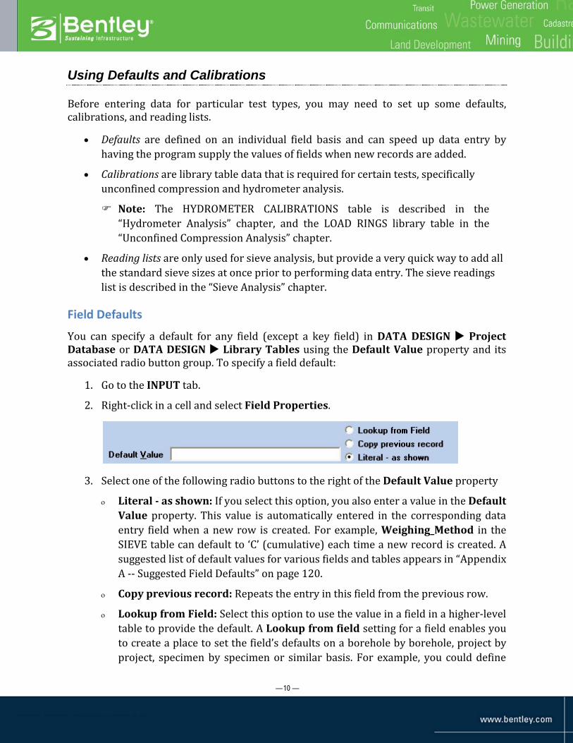
You can specify a default for any field (except a key field) in DATA DESIGN Project Database or DATA DESIGN Library Tables using the Default Value property and its associated radio button group. To specify a field default:
1. Go to the INPUT tab.
2. Right-click in a cell and select Field Properties.
3. Select one of the following radio buttons to the right of the Default Value property
ο Literal - as shown: If you select this option, you also enter a value in the Default Value property. This value is automatically entered in the corresponding data entry field when a new row is created. For example, Weighing_Method in the SIEVE table can default to ‘C’ (cumulative) each time a new record is created. A suggested list of default values for various fields and tables appears in “Appendix A -- Suggested Field Defaults” on page 120.
ο Copy previous record: Repeats the entry in this field from the previous row.
ο Lookup from Field: Select this option to use the value in a field in a higher-level table to provide the default. A Lookup from field setting for a field enables you to create a place to set the field’s defaults on a borehole by borehole, project by project, specimen by specimen or similar basis. For example, you could define
— 11 —
master Diameter and Height fields in the POINT table for the WC DENSITY fields of the same names, and reference the POINT table fields from the Field Properties in the WC DENSITY fields. When you enter values in the POINT record for a borehole, this would establish defaults for all WC DENSITY records for the borehole.
Note that after setting up defaults for fields in various tables, you should save your current database structure to your data template. This enables the same defaults to be established in any project subsequently cloned from the data template.
— 12 —
Lab Testing User Interface
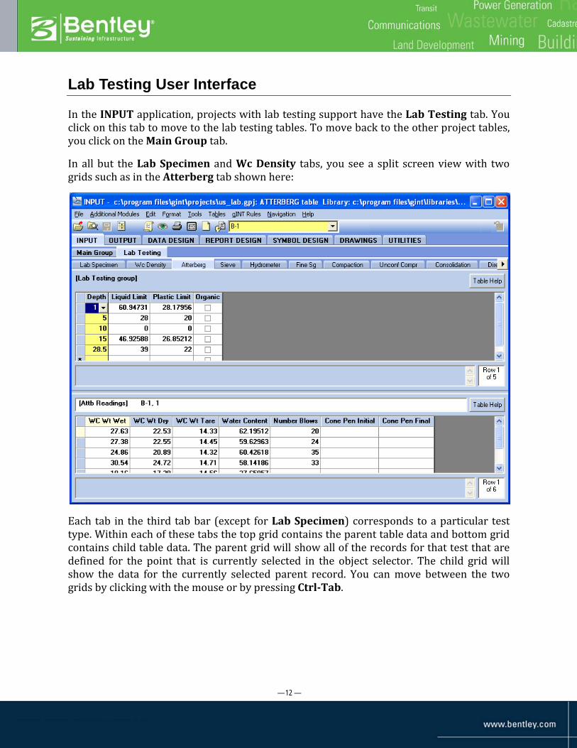
In the INPUT application, projects with lab testing support have the Lab Testing tab. You click on this tab to move to the lab testing tables. To move back to the other project tables, you click on the Main Group tab.
In all but the Lab Specimen and Wc Density tabs, you see a split screen view with two grids such as in the Atterberg tab shown here:
Each tab in the third tab bar (except for Lab Specimen) corresponds to a particular test type. Within each of these tabs the top grid contains the parent table data and bottom grid contains child table data. The parent grid will show all of the records for that test that are defined for the point that is currently selected in the object selector. The child grid will show the data for the currently selected parent record. You can move between the two grids by clicking with the mouse or by pressing Ctrl-Tab.

— 13 —
Relational Database Structure
The following diagram illustrates the parent-child relationship structure of all standard lab testing tables, using the standard database diagram symbols for one-to-many ( ) and one-to-one ( ).
As can be seen from the diagram, there are potentially many LAB SPECIMEN records for each POINT record (each LAB SPECIMEN record represents a specimen from a different depth within the borehole). Also, all of the tables in the third column (WC DENSITY, ATTERBERG, and so on) have a one-to-one relationship with LAB SPECIMEN. In other words, these Column 3 tables enable the creation of records that have the same PointID-Depth combination as some LAB SPECIMEN record. Tables in Column 4 are one-to-many children of particular Column 3 tables, and provide the ability to enter individual readings that are summarized in the parent record. For example, each SIEVE record can have multiple SV READINGS children.

— 14 —
Note: It is not required for LAB SPECIMEN to be a child of POINT; it could be the child of another table. Refer to “Making LAB SPECIMEN a Child of a Non-POINT Table” on page 124.
— 15 —
Lab Testing Tables
Defining a Lab Specimen
The LAB SPECIMEN table is the parent for all the lab testing tables. The PointID and Depth of each test specimen must be defined here before any data can be input elsewhere, with the following exception: if you add a record to one of the lab testing tables and that PointID-Depth combination was not defined in LAB SPECIMEN, gINT will show a message that it does not exist and allow you to add it to LAB SPECIMEN on the fly. For example, let's say you enter data in the Sieve tab for PointID = ‘B-1’ at Depth = 5, and then save. If a record at B-1 depth 5 was not defined in the Lab Specimen tab, gINT will show a message that it does not exist and ask if you wish to add it.
At least one specimen must be defined in the LAB SPECIMEN table before the program will allow you to move to the other lab testing tables.
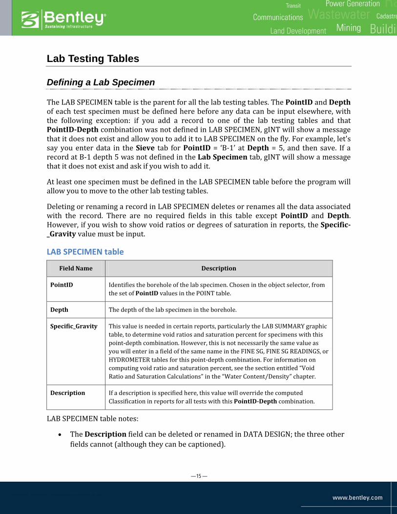
Deleting or renaming a record in LAB SPECIMEN deletes or renames all the data associated with the record. There are no required fields in this table except PointID and Depth. However, if you wish to show void ratios or degrees of saturation in reports, the Specific-_Gravity value must be input.
LAB SPECIMEN table
Field Name Description
PointID Identifies the borehole of the lab specimen. Chosen in the object selector, from the set of PointID values in the POINT table.
Depth The depth of the lab specimen in the borehole.
Specific_Gravity This value is needed in certain reports, particularly the LAB SUMMARY graphic table, to determine void ratios and saturation percent for specimens with this point-depth combination. However, this is not necessarily the same value as you will enter in a field of the same name in the FINE SG, FINE SG READINGS, or HYDROMETER tables for this point-depth combination. For information on computing void ratio and saturation percent, see the section entitled “Void Ratio and Saturation Calculations” in the “Water Content/Density” chapter.
Description If a description is specified here, this value will override the computed Classification in reports for all tests with this PointID-Depth combination.
LAB SPECIMEN table notes:
• The Description field can be deleted or renamed in DATA DESIGN; the three other fields cannot (although they can be captioned).

— 16 —
Some Typical Reports
This table is not directly reported in any reports.

— 17 —
Water Content / Density
Background
Water content (or moisture content) is the quantity of water contained in soil or rock on a volumetric or gravimetric basis. The property is expressed as a ratio, which can range from zero (completely dry) to the value of the material’s porosity at saturation. Water content is calculated by dividing the volume of the water by the total volume of the sample. Density is mass m per unit volume V—how heavy something is compared to its size. This feature can be used to determine what optimum water content correlates with the maximum dry density.
Data Entry
The Wc Density tab is for data entry in the WC DENSITY table. You need to have a parent LAB SPECIMEN record for the desired depth to create a WC DENSITY record (or you can create it on the fly).
Any or all of the three final results fields (Water_Content, Wet_Density and Dry_Density) can be input directly. If the data exists in other fields for calculating these values, the program will do so and overwrite any values that are in those fields. Clicking the Save icon generates values in any fields that are calculated.
Note that the Diameter and Height must be in millimeters and the weight of the total specimen (Wt_Spec_Tare) and its tare (Wt_Tare) must be in grams. The weights for the Water Content determination can be in any consistent units, that is, WC_Wt_Wet, WC_Wt_Dry and WC_Wt_Tare can all be in grams, all be in pounds, etc.
The calculated densities are determined using the Water Unit Weight value in the PROJECT table. For example, a Water Unit Weight of 62.42796 generates densities in pounds/cubic foot, whereas a value of 1 generates values in grams/cu cm. Densities cannot be calculated without a value in that field. Changing the Water Unit Weight will not change existing results—you must recalculate by saving (or selecting gINT Rules Recalculate Current Table).
The specifics of the calculations are in “Data Entry Scenarios and Calculations” on page 19.
— 18 —
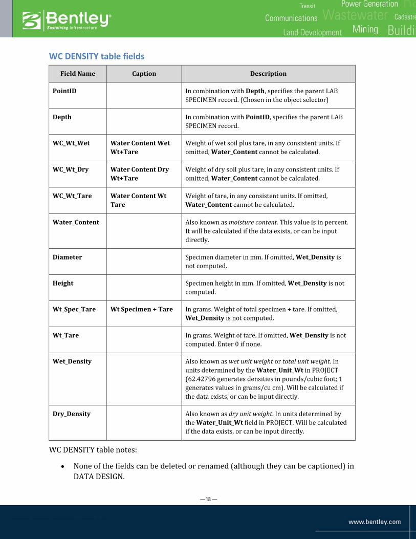
WC DENSITY table fields
Field Name Caption Description
PointID In combination with Depth, specifies the parent LAB SPECIMEN record. (Chosen in the object selector)
Depth In combination with PointID, specifies the parent LAB SPECIMEN record.
WC_Wt_Wet Water Content Wet Wt+Tare
Weight of wet soil plus tare, in any consistent units. If omitted, Water_Content cannot be calculated.
WC_Wt_Dry Water Content Dry Wt+Tare
Weight of dry soil plus tare, in any consistent units. If omitted, Water_Content cannot be calculated.
WC_Wt_Tare Water Content Wt Tare
Weight of tare, in any consistent units. If omitted, Water_Content cannot be calculated.
Water_Content Also known as moisture content. This value is in percent. It will be calculated if the data exists, or can be input directly.
Diameter Specimen diameter in mm. If omitted, Wet_Density is not computed.
Height Specimen height in mm. If omitted, Wet_Density is not computed.
Wt_Spec_Tare Wt Specimen + Tare In grams. Weight of total specimen + tare. If omitted, Wet_Density is not computed.
Wt_Tare In grams. Weight of tare. If omitted, Wet_Density is not computed. Enter 0 if none.
Wet_Density Also known as wet unit weight or total unit weight. In units determined by the Water_Unit_Wt in PROJECT (62.42796 generates densities in pounds/cubic foot; 1 generates values in grams/cu cm). Will be calculated if the data exists, or can be input directly.
Dry_Density Also known as dry unit weight. In units determined by the Water_Unit_Wt field in PROJECT. Will be calculated if the data exists, or can be input directly.
WC DENSITY table notes:
• None of the fields can be deleted or renamed (although they can be captioned) in DATA DESIGN.

— 19 —
• No fields have an associated lookup
Data Entry Scenarios and Calculations
Calculations are per ASTM D2216.
Water Content Calculations
There are three ways to calculate Water_Content:
• From WC_Wt_Wet, WC_Wt_Dry and WC_Wt_Tare.
Example:
Entered Calculated
WC_Wt_Wet WC_Wt_Dry WC_Wt_Tare Water_Content
95.3 80 20.2 25.59%
• From Wet_Density and Dry_Density:
Example:
Entered Calculated
Wet_Density Dry_Density Water_Content
133.2 115.424 15.40%
• From Dry_Density and source fields for Wet_Density (Diameter, Height, Wt_Spec_Tare, and Wt_Tare)
(see Wet_Density calculations, below)
Wet Density Calculations
Wet_Density (also known as total unit weight or wet unit weight) can be calculated in either of two ways:
• From Diameter, Height, Wt_Spec_Tare, Wt_Tare and Water_Unit_Wt:
Cubic cm example:

— 20 —
Entered Calculated
Diameter (mm)
Height (mm)
Wt_Spec_ Tare (g)
Wt_ Tare (g)
area sq cm
volume cu cm
Water_ Unit_Wt
Wet_ Density
50.8 152.4 655.7 0 20.2683 308.8889 62.42796 132.52
Cubic ft example:
Entered Calculated
Diameter (mm)
Height (mm)
Wt_Spec_ Tare
(g)
Wt_ Tare
(g)
net wt spec lbs
area sq ft volume cu ft
Water_ Unit_Wt
Wet_ Density
50.8 152.4 655.7 0 1.445571 0.021817 0.010908 1 132.52
• From Water_Content and Dry_Density:
Example:
Entered Calculated
Dry_Density Water_Content Wet_Density
101.26 23.98% 125.54

— 21 —
Dry Density Calculations
Dry_Density (also known as dry unit weight) can be calculated from the following:
• From Water_Content and Wet_Density:
Example:
Entered Calculated
Water_Content Wet_Density Dry_Density
31.32% 119.5 90.999
• From Water_Content and Wet_Density’s source fields (Diameter, Height, Wt_Spec_Tare, and Wt_Tare)
(see “Wet Density Calculations,” above)
• From Wet_Density and Water_Content’s source fields (WC_Wt_Wet, WC_Wt_Dry and WC_Wt_Tare)
(see “Water Content Calculations,” above)
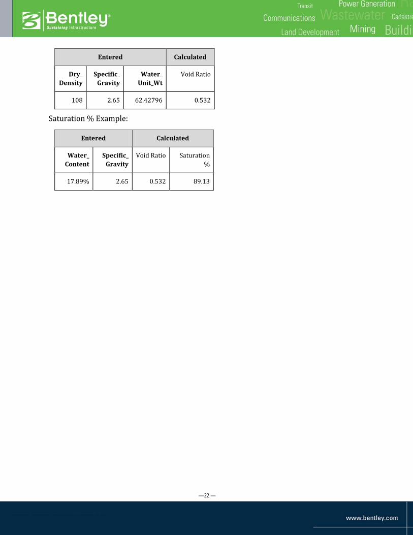
Void Ratio and Saturation Calculations
Void Ratio and Saturation % are calculated values displayed in reports, primarily the LAB SUMMARY graphic table. They are calculated via the Rep_Void_Ratio and Rep_Saturation user system data items respectively, and are derived from the Water_Content and Dry_Density values in the current WC DENSITY record, as well as Water_Unit_Wt in PROJECT (to establish the units for densities) and Specific_Gravity in LAB SPECIMEN.
Note: If there is no Specific_Gravity value in the parent LAB SPECIMEN record, Void Ratio and Saturation % are not calculated. Also, note that if Dry_Density is missing from the WC DENSITY record, the Dry_Density field in UNCONF COMPRESS, then CONSOLIDATION, then DIRECT SHEAR is accessed until a value is found (refer to the Rep_Dry_Density user system data item in the library for details).
Void Ratio Example:
— 22 —
Entered Calculated
Dry_ Density
Specific_ Gravity
Water_ Unit_Wt
Void Ratio
108 2.65 62.42796 0.532
Saturation % Example:
Entered Calculated
Water_ Content
Specific_ Gravity
Void Ratio Saturation %
17.89% 2.65 0.532 89.13

— 23 —
Some Typical Reports
LAB_SUMMARY (Summary of Laboratory Results ) graphic table/text table
In standard libraries (such as ‘gint std US.glb’) water content and wet and dry density values are reported for each borehole-depth combination using the US_LAB_SUMMARY (Summary of Laboratory Results) graphic text doc and text doc. They appear directly in the Water Content and Dry Density columns, and indirectly through computations in the Saturation and Void Ratio columns.

— 24 —
GEOTECH BH PLOTS Log
The plot-vs-depth column at right in this log report graphs, among other things, moisture content (filled circle markers) against plastic limit to liquid limit horizontal range lines.

— 25 —
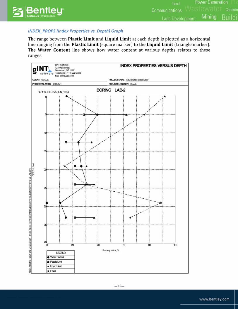
INDEX_PROPS (Index Properties vs. Depth) Graph
Water_Content is also plotted as one curve in the Index Properties vs. Depth (INDEX_PROPS) graph. Notice the solid zig-zag line curve with filled circle data markers below.

— 26 —
Atterberg Analysis
Background
Atterberg limits are a basic measure of the nature of a fine-grained soil. Depending on the water content of the soil, it may appear in four states: solid, semi-solid, plastic and liquid. In each state the consistency and behavior of a soil is different and thus so are its engineering properties. Therefore, the boundary between each state can be defined based on a change in the soil's behavior. The Atterberg limits can be used to distinguish between silt and clay, and they can distinguish between different types of silts and clays.
The plastic limit (PL) is the water content where soil starts to exhibit plastic behavior. A thread of soil is at its plastic limit when it is rolled to a diameter of 3 mm and crumbles. To improve consistency, a 3 mm diameter rod is often used to gauge the thickness of the thread when conducting the test.
The liquid limit (LL) is the water content where a soil changes from plastic to liquid behavior. The original liquid limit test of Atterberg's involved mixing a pat of clay in a round-bottomed porcelain bowl of 10-12 cm diameter. A groove was cut through the pat of clay with a spatula, and the bowl was then struck many times against the palm of one hand.
Casagrande subsequently standardized the apparatus and the procedures to make the liquid limit measurement more repeatable. In the Casagrande method, soil is placed into the metal cup portion of the device and a groove is made down its center with a standardized tool. The cup is repeatedly dropped 10mm onto a hard rubber base until the groove is closed for 13 mm (½ inch). The moisture content at which it takes 25 drops of the cup to cause the groove to close is defined as the liquid limit.
Another method for measuring the liquid limit is the cone penetrometer test. It is based on the measurement of penetration into the soil of a standardized cone of specific mass. Despite the universal prevalence of the Casagrande method, the cone penetrometer is often considered to be a more consistent alternative because it minimizes the possibility of human variations when carrying out the test.
The plasticity index (PI) is a measure of the plasticity of a soil. It is the size of the range of water contents where the soil exhibits plastic properties. The PI is the difference between the liquid limit and the plastic limit (PI = LL - PL). Soils with a high PI tend to be clay, those with a lower PI tend to be silt, and those with a PI of 0 tend to have little or no silt or clay.
The liquidity index (LI) is used for scaling the natural water content of a soil sample to the limits. It can be calculated as a ratio of difference between natural water content, plastic limit, and plasticity index: LI=(W-PL)/(LL-PL) where W is the natural water content.
The activity (A) of a soil is the PI divided by the percent of clay-sized particles present. Different types of clays have differing specific surface areas. This controls how much wetting is required to move a soil from one phase to another, such as across the liquid limit or the plastic limit. From the activity, one can predict the dominant clay type present in a

— 27 —
soil sample. High activity signifies large volume change when wetted and large shrinkage when dried. Soils with high activity are very reactive chemically.
Normally, activity of clay is between 0.75 and 1.25. It is assumed that the plasticity index is approximately equal to the clay fraction (A = 1). When A is less than 0.75, it is considered inactive. When it is greater than 1.25, it is considered active.
Data Entry
The Atterberg tab is for data entry into the ATTERBERG (parent) and ATTB READINGS (child) tables. One ATTERBERG table record can be created for each borehole-depth combination present in its parent (the LAB SPECIMEN table). The ATTERBERG record holds data that applies to or is calculated from all of its child (ATTB READINGS) records. Multiple ATTB READINGS records can be created for an ATTERBERG record, and each holds data from one plastic limit reading, or one liquid limit test performed with a Casagrande cup or cone penetrometer, for the parent’s borehole-depth combination.
Liquid_Limit and Plastic_Limit can be input directly in the ATTERBERG (parent) record. Alternately, if ATTB READINGS records exist for an ATTERBERG record, the Liquid_Limit and Plastic_Limit in the parent will be calculated from its set of child records.
In the ATTB READINGS (child) table, the Water_Content for each reading is calculated from the WC_Wt_Wet, WC_Wt_Dry, and WC_Wt_Tare fields (all three must be provided), or can be entered directly. Water_Content, or values for the three source fields to compute it, must be present in every ATTB READINGS record. For plastic limit tests, this is all that is entered. For liquid limit tests, you also enter either a value for Number_Blows (when using the Casagrande cup method) or Cone_Pen_Initial and Cone_Pen_Final (when using the cone penetrometer method). Note that Casagrande cup and cone penetrometer tests cannot be combined for the same borehole-depth combination.
In the lower grid you can enter 1) only liquid limit, 2) only plastic limit readings, or 3) both liquid and plastic limit readings. The program automatically inserts a zero into the upper grid for the item that is not input in the lower grid, for example, if only liquid limit readings are input in the lower grid, the calculated Liquid_Limit will be inserted in the upper grid and zero will be inserted for the Plastic_Limit.

— 28 —
Note: This is to accommodate ASTM specification D 4318 (Liquid Limit, Plastic Limit, and Plasticity Index of Soils), section 20.1.4 which states in part: "If the Liquid Limit or Plastic Limit tests could not be performed, or if the Plastic Limit is equal to or greater than the Liquid Limits, report the soil as nonplastic, NP." In southeastern Alaska there are soils where the Liquid Limit test can be performed and yields values in the range of 20 but the Plastic Limit test cannot be run. Your first reaction might be to input a value of "0" and expect the ASTM functions to classify such a soil as a clay since the PI would be 20. Section 20.1.4 says otherwise, that is, since the Plastic Limit test could not be run the soil is non-plastic and therefore a silt. The ASTM Classification function in gINT accommodates this condition.
For additional details on calculations, see “Data Entry Scenarios and Calculations” on page 30.
ATTERBERG table fields
Field Name Description
PointID In combination with Depth, specifies the parent LAB SPECIMEN record. (Specified in the object selector).
Depth In combination with PointID, specifies the parent LAB SPECIMEN record.
Liquid_Limit In %. Calculated from the data in liquid limit-type readings records in ATTB READINGS (records with either blows or cone penetrometer values). Alternately, this can be directly entered in ATTERBERG, but the manually entered value will be overwritten if there is child liquid limit data. For Casagrande cup (blows) data, any number of readings can be provided. For cone penetrometer data, a minimum of three readings is required.
Plastic_Limit In %. Calculated from the data in plastic limit-type readings records in ATTB READINGS (records lacking blows and cone penetrometer values). Alternately, this can be directly entered in ATTERBERG, but the manually entered value will be overwritten if there is child plastic limit data.
Organic Affects the ASTM classification in reports.
ATTERBERG table notes:
• None of the fields can be deleted or renamed (although they can be captioned) in DATA DESIGN.
• None of the fields have captions • There are no associated lookups
— 29 —
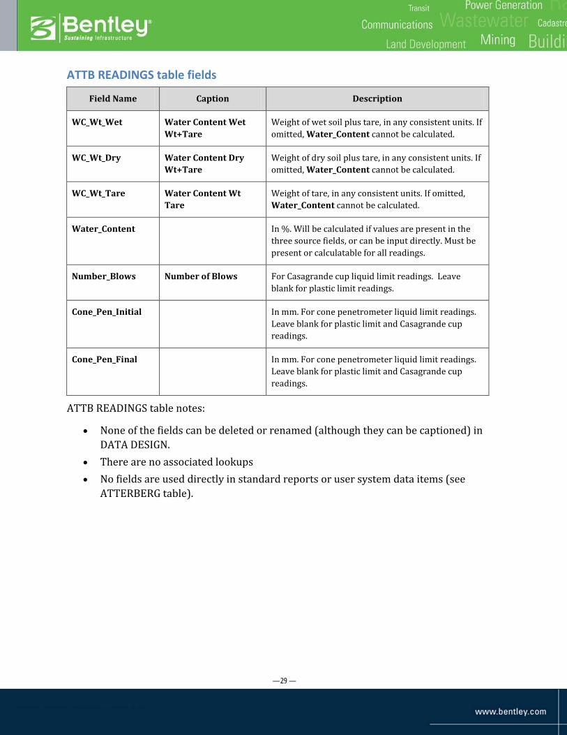
ATTB READINGS table fields
Field Name Caption Description
WC_Wt_Wet Water Content Wet Wt+Tare
Weight of wet soil plus tare, in any consistent units. If omitted, Water_Content cannot be calculated.
WC_Wt_Dry Water Content Dry Wt+Tare
Weight of dry soil plus tare, in any consistent units. If omitted, Water_Content cannot be calculated.
WC_Wt_Tare Water Content Wt Tare
Weight of tare, in any consistent units. If omitted, Water_Content cannot be calculated.
Water_Content In %. Will be calculated if values are present in the three source fields, or can be input directly. Must be present or calculatable for all readings.
Number_Blows Number of Blows For Casagrande cup liquid limit readings. Leave blank for plastic limit readings.
Cone_Pen_Initial In mm. For cone penetrometer liquid limit readings. Leave blank for plastic limit and Casagrande cup readings.
Cone_Pen_Final In mm. For cone penetrometer liquid limit readings. Leave blank for plastic limit and Casagrande cup readings.
ATTB READINGS table notes:
• None of the fields can be deleted or renamed (although they can be captioned) in DATA DESIGN.
• There are no associated lookups • No fields are used directly in standard reports or user system data items (see
ATTERBERG table).
— 30 —
Data Entry Scenarios and Calculations
Atterberg indices and soil classification are covered in ASTM D2487.
Scenario 1: Liquid Limit and Plastic Limit Values Directly Entered
This is the simplest case. You can directly enter Liquid_Limit and Plastic_Limit values in the parent ATTERBERG table, and these will be used in reporting if nothing is entered in the lower grid. However, if data is entered in child ATTB READINGS records from which parent Liquid_Limit or Plastic_Limit values can be calculated, the calculated parent values will overwrite the entered parent values on saving.
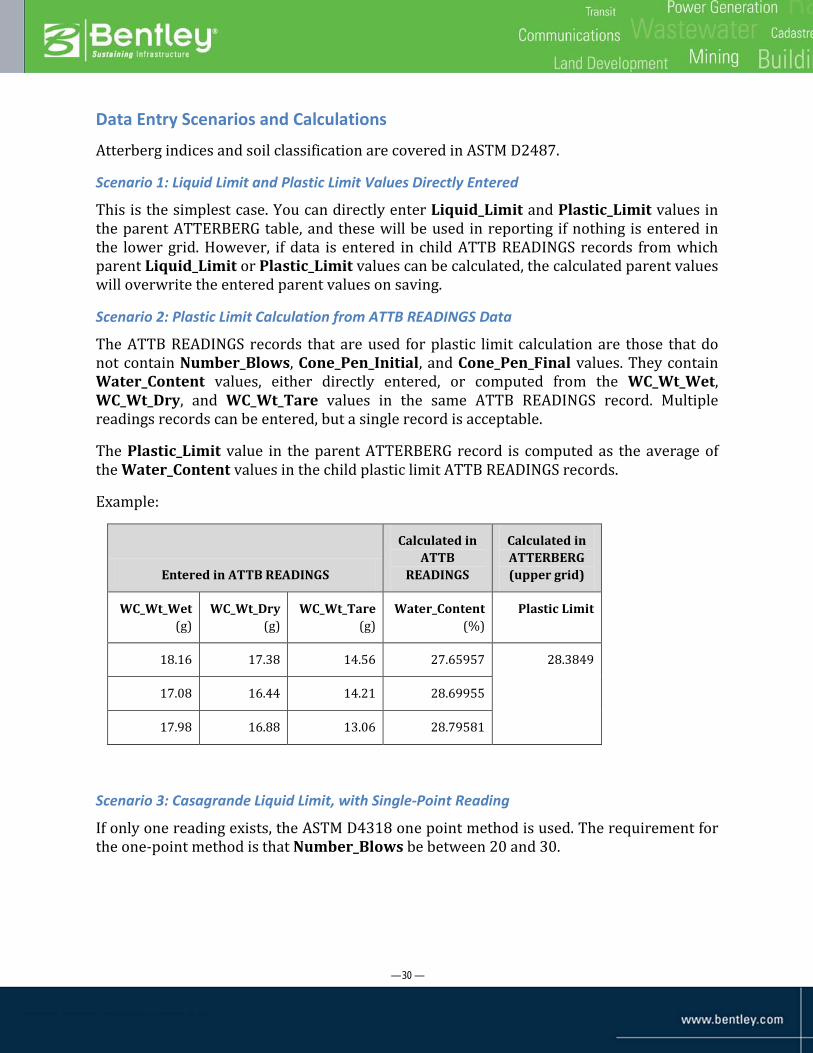
Scenario 2: Plastic Limit Calculation from ATTB READINGS Data
The ATTB READINGS records that are used for plastic limit calculation are those that do not contain Number_Blows, Cone_Pen_Initial, and Cone_Pen_Final values. They contain Water_Content values, either directly entered, or computed from the WC_Wt_Wet, WC_Wt_Dry, and WC_Wt_Tare values in the same ATTB READINGS record. Multiple readings records can be entered, but a single record is acceptable.
The Plastic_Limit value in the parent ATTERBERG record is computed as the average of the Water_Content values in the child plastic limit ATTB READINGS records.
Example:
Entered in ATTB READINGS
Calculated in ATTB
READINGS
Calculated in ATTERBERG (upper grid)
WC_Wt_Wet (g)
WC_Wt_Dry (g)
WC_Wt_Tare (g)
Water_Content (%)
Plastic Limit
18.16 17.38 14.56 27.65957 28.3849
17.08 16.44 14.21 28.69955
17.98 16.88 13.06 28.79581
Scenario 3: Casagrande Liquid Limit, with Single-Point Reading
If only one reading exists, the ASTM D4318 one point method is used. The requirement for the one-point method is that Number_Blows be between 20 and 30.
— 31 —
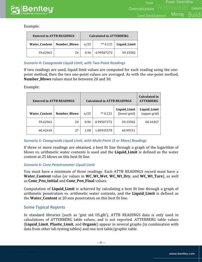
Example:
Entered in ATTB READINGS Calculated in ATTERBERG
Water_Content Number_Blows n/25 ** 0.121 Liquid_Limit
59.62963 24 0.96 0.99507272 59.33582
Scenario 4: Casagrande Liquid Limit, with Two-Point Readings
If two readings are used, liquid limit values are computed for each reading using the one-point method, then the two one-point values are averaged. As with the one-point method, Number_Blows values must be between 20 and 30.
Example:
Entered in ATTB READINGS Calculated in ATTB READINGS Calculated in ATTERBERG
Water_Content Number_Blows n/25 ** 0.121 Liquid_Limit
(lower grid) Liquid_Limit
(upper grid)
59.62963 24 0.96 0.99507272 59.33582 60.16367
60.42618 27 1.08 1.00935578 60.99151
Scenario 5: Casagrande Liquid Limit, with Multi-Point (3 or More) Readings
If three or more readings are obtained, a best fit line through a graph of the logarithm of blows vs. arithmetic water contents is used and the Liquid_Limit is defined as the water content at 25 blows on this best fit line.
Scenario 6: Cone Penetrometer Liquid Limit
You must have a minimum of three readings. Each ATTB READINGS record must have a Water_Content value (or values in WC_Wt_Wet, WC_Wt_Dry, and WC_Wt_Tare), as well as Cone_Pen_Initial and Cone_Pen_Final values.
Computation of Liquid_Limit is achieved by calculating a best fit line through a graph of arithmetic penetration vs. arithmetic water contents, and the Liquid_Limit is defined as the Water_Content at 20 mm penetration on this best fit line.
Some Typical Reports
In standard libraries (such as ‘gint std US.glb’), ATTB READINGS data is only used in calculations of ATTERBERG table values, and is not reported. ATTERBERG table values (Liquid_Limit, Plastic_Limit, and Organic) appear in several graphs (in combination with data from other lab testing tables) and one text table/graphic table.

— 32 —
ATTERBERG_LIMITS (Atterberg Limits Results) graph
The graph in the upper portion plots plasticity index (liquid limit less plastic limit) against plastic limit for each point-depth combination in the ATTERBERG table.
Beneath the plot, the graphic table reports liquid limit, plastic limit, and plasticity index data by each borehole-depth combination. Fines and Classification are additionally reported if there is percent finer and reading (sieve size) data available from the SV READINGS (sieve analysis) table.
— 33 —
INDEX_PROPS (Index Properties vs. Depth) Graph
The range between Plastic Limit and Liquid Limit at each depth is plotted as a horizontal line ranging from the Plastic Limit (square marker) to the Liquid Limit (triangle marker). The Water Content line shows how water content at various depths relates to these ranges.

— 34 —
LAB SUMMARY (Summary of Laboratory Results) graphic table/text table
This table reports Atterberg liquid limit, plastic limit, and plasticity index data regardless of whether there is data in other tables.
— 35 —
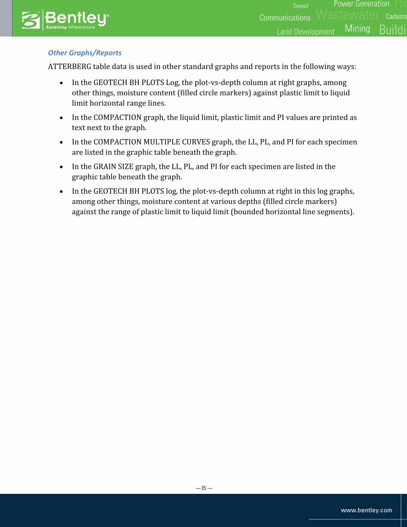
Other Graphs/Reports
ATTERBERG table data is used in other standard graphs and reports in the following ways:
• In the GEOTECH BH PLOTS Log, the plot-vs-depth column at right graphs, among other things, moisture content (filled circle markers) against plastic limit to liquid limit horizontal range lines.
• In the COMPACTION graph, the liquid limit, plastic limit and PI values are printed as text next to the graph.
• In the COMPACTION MULTIPLE CURVES graph, the LL, PL, and PI for each specimen are listed in the graphic table beneath the graph.
• In the GRAIN SIZE graph, the LL, PL, and PI for each specimen are listed in the graphic table beneath the graph.
• In the GEOTECH BH PLOTS log, the plot-vs-depth column at right in this log graphs, among other things, moisture content at various depths (filled circle markers) against the range of plastic limit to liquid limit (bounded horizontal line segments).
— 36 —
Sieve Analysis
Background
A sieve analysis is a procedure used to assess the particle size distribution of a granular material. The size distribution is often of critical importance to the way the material performs in use. It can be used for any type of non-organic or organic granular round materials including sands, clays, coal, soil, crushed granite or feldspars, and a wide range of manufactured powders.
For coarse material (sizes that range down to #200 mesh, that is, 75 μm) a sieve analysis and particle size distribution is accurate and consistent. However, for material that is finer than #200 mesh, dry sieving is significantly less accurate. This is because the mechanical energy required to make particles pass through an opening and the surface attraction effects between the particle and the screen increase as the particle size decreases. To determine particle size distribution for these finest sizes, hydrometer analysis is performed.
Sediment samples may undergo grain size analysis through sieves. Graphing the cumulative weight percent retained vs. passing grain size (sieve number) will result in the sediment grain-size distribution curve. The grain-size distribution curve is used to quantitatively classify the sediment type.
Data Entry
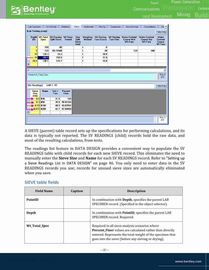
The Sieve tab is for data entry in the SIEVE and SV READINGS tables. One SIEVE table record can be created for each borehole-depth combination present in the LAB SPECIMEN table and holds data that applies to all of its child (SV READINGS) records. Multiple SV READINGS records are created for a SIEVE record, and each holds data from one sieve reading obtained for the parent’s borehole-depth combination.
— 37 —
A SIEVE (parent) table record sets up the specifications for performing calculations, and its data is typically not reported. The SV READINGS (child) records hold the raw data, and most of the resulting calculations, from tests.
The readings list feature in DATA DESIGN provides a convenient way to populate the SV READINGS table with child records for each new SIEVE record. This eliminates the need to manually enter the Sieve Size and Name for each SV READINGS record. Refer to “Setting up a Sieve Readings List in DATA DESIGN” on page 46. You only need to enter data in the SV READINGS records you use; records for unused sieve sizes are automatically eliminated when you save.
SIEVE table fields
Field Name Caption Description
PointID In combination with Depth, specifies the parent LAB SPECIMEN record. (Specified in the object selector).
Depth In combination with PointID, specifies the parent LAB SPECIMEN record. Required.
Wt_Total_Spec Required in all sieve analysis scenarios where Percent_Finer values are calculated rather than directly entered. Represents the total weight of the specimen that goes into the sieve (before any sieving or drying).

— 38 —
Field Name Caption Description
Wt_Passing_ Split_Sieve
This value is calculated in all scenarios, following a Save. In unsplit specimens, it represents the total weight of the specimen that passed the sieves, that is, the total weight of the specimen less the weight retained in the sieves.
In split specimens, it is the weight of the specimen less the weight of material coarse-sieved. For example, if the smallest coarse sieve is #10, this value will be the weight of the portion that passes the #10 sieve.
Wt_Fines_Tested With unsplit specimens, this field is not used; for split sieve specimens it is required. It specifies the weight of the fraction from the original specimen used for sieving in fine sieves.
Size_Split_Sieve With unsplit specimens, this field is not used; for split sieve specimens it is required, and specifies the size of the smallest sieve included in coarse sieving, in mm. For example, if the smallest coarse sieve is #10, this value would be 2 (mm).
Weighing_Method Specifies how Soil_Tare values in the child records are interpreted. The options are C for cumulative and I for incremental. Cumulative weighing sums the weights of soil retained on each sieve and those coarser. Incremental weighing only records the weight retained on each sieve individually. This is the same for split and unsplit specimens.
Wt_Sieving_ Tare_Coarse
With unsplit specimens, this field is not used; for split sieve specimens it is required. Used for entry of a single tare value (that applies to all sieves) when there is no split. Tare values are entered separately in Wt_Sieving_Tare_Coarse (applying to the coarse sieves) and Wt_Sieving_Tare_Fine (applying to the fine sieves) when split. This is the default setup for sieve analysis in gINT. However if you need to specify different tare weights for the various sieves, this can be done by adding a Wt_Sieve_Tare field in SV_READINGS.
Wt_Sieving_Tare_Fine Required when split sieving. Tare weight for all fine sieves (see Wt_Sieving_Tare_Coarse).

— 39 —
Field Name Caption Description
WC_Wt_Wet_Coarse Water Content Coarse Wet Wt+Tare
Wet weight, including tare, for moisture content adjustment of an unsplit specimen or the coarse fraction of a split specimen. To utilize a wet total weight in an unsplit specimen requires the use of three fields: WC_Wt_Wet_Coarse, WC_Wt_Dry_Coarse, and WC_Wt_Tare_Coarse (all using the same units). In a split specimen, the corresponding three _Fine fields are also required. The principle is that some portion of the soil sample is set aside for moisture content testing. The weighing dish is weighed to establish the tare value, and the moist sample on the dish is weighed to establish the wet weight with tare (this value). The sample is heated to vaporize the moisture, and it is re-weighed. The difference between the wet and dry weights is the weight of the moisture lost, and the ratio of the lost moisture to the weight of the dry sample is the moisture content percentage (saved as Water_Content_Coarse). This percentage can then be used to convert dry Soil_Tare weights into equivalent wet weights for calculation of Percent_Finer values.
WC_Wt_Dry_Coarse Water Content Coarse Dry Wt+Tare
Dry weight, including tare, for moisture content adjustment of an unsplit specimen or the coarse fraction of a split specimen. See WC_Wt_Wet_Coarse.
WC_Wt_Tare_Coarse Water Content Coarse Wt Tare
Tare weight for moisture content adjustment of an unsplit specimen or the coarse fraction of a split specimen. See WC_Wt_Wet_Coarse.
Water_Content_Coarse
Moisture content percentage calculated for an unsplit wet specimen or the coarse fraction of a split wet specimen. See WC_Wt_Wet_Coarse.
WC_Wt_Wet_Fine Water Content Fine Wet Wt+Tare
Wet weight, including tare, for moisture content adjustment of the fine fraction of a split specimen. See WC_Wt_Wet_Coarse. With unsplit specimens this field is not used.
WC_Wt_Dry_ Fine Water Content Fine Dry Wt+Tare
Dry weight, including tare, for moisture content adjustment of the fine fraction of a split specimen. See WC_Wt_Wet_Coarse. With unsplit specimens this field is not used.
WC_Wt_Tare_ Fine Water Content Fine Wt Tare
Tare weight for moisture content adjustment of the fine fraction of a split specimen. See WC_Wt_Wet_Coarse. With unsplit specimens this field is not used.
— 40 —
Field Name Caption Description
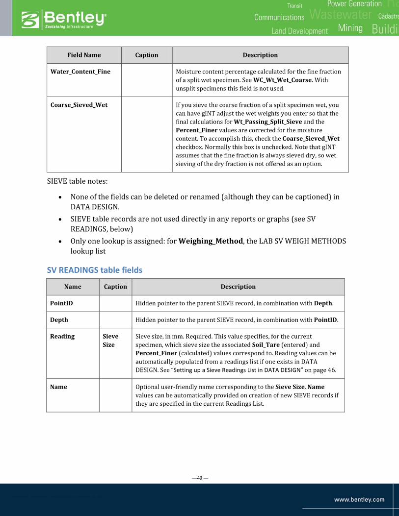
Water_Content_Fine Moisture content percentage calculated for the fine fraction of a split wet specimen. See WC_Wt_Wet_Coarse. With unsplit specimens this field is not used.
Coarse_Sieved_Wet If you sieve the coarse fraction of a split specimen wet, you can have gINT adjust the wet weights you enter so that the final calculations for Wt_Passing_Split_Sieve and the Percent_Finer values are corrected for the moisture content. To accomplish this, check the Coarse_Sieved_Wet checkbox. Normally this box is unchecked. Note that gINT assumes that the fine fraction is always sieved dry, so wet sieving of the dry fraction is not offered as an option.
SIEVE table notes:
• None of the fields can be deleted or renamed (although they can be captioned) in DATA DESIGN.
• SIEVE table records are not used directly in any reports or graphs (see SV READINGS, below)
• Only one lookup is assigned: for Weighing_Method, the LAB SV WEIGH METHODS lookup list
SV READINGS table fields
Name Caption Description
PointID Hidden pointer to the parent SIEVE record, in combination with Depth.
Depth Hidden pointer to the parent SIEVE record, in combination with PointID.
Reading Sieve Size
Sieve size, in mm. Required. This value specifies, for the current specimen, which sieve size the associated Soil_Tare (entered) and Percent_Finer (calculated) values correspond to. Reading values can be automatically populated from a readings list if one exists in DATA DESIGN. See “Setting up a Sieve Readings List in DATA DESIGN” on page 46.
Name Optional user-friendly name corresponding to the Sieve Size. Name values can be automatically provided on creation of new SIEVE records if they are specified in the current Readings List.

— 41 —
Name Caption Description
Soil_Tare Soil + Tare
Entered for each sieve size with data. If incremental weighing, enter the weight retained on each sieve; if cumulative, enter the sum of the weights on this sieve and those coarser. Enter dry weights only (unless performing wet sieving of the coarse fraction and Coarse_Sieved_Wet is checked, in which case you enter wet weights for the coarse fraction and dry weights for the fine).
Percent_Finer When you save, Percent_Finer is calculated for each SV READINGS record with a Soil_Tare value. The resulting set of values will vary depending on the settings in the parent SIEVE record. Alternately, Percent_Finer values can be entered directly, if you do not need them calculated.
SV READINGS table notes:
• None of the fields can be deleted or renamed (although they can be captioned) in DATA DESIGN.
• No associated lookups.
Data Entry Scenarios and Calculations
Various data entry scenarios are possible, depending on your needs. The most common ones, unsplit sieve and split sieve without moisture calculations, are described below (in addition to the non-calculated scenario, direct entry of Percent_Finer values). More complicated scenarios involving wet specimens are described in “Appendix C -- Scenarios using Wet Specimens in Sieve Analysis” on page 127.
The calculations for sieve analysis are detailed in ASTM D422.
Scenario 1: Percent Finer values directly entered
If the Percent Finer (Percent_Finer) values are directly entered into the SV READINGS grid, nothing is required in the parent record except Depth, and no calculations are performed.
— 42 —
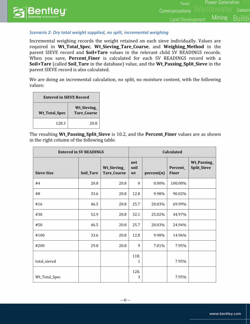
Scenario 2: Dry total weight supplied, no split, incremental weighing
Incremental weighing records the weight retained on each sieve individually. Values are required in Wt_Total_Spec, Wt_Sieving_Tare_Coarse, and Weighing_Method in the parent SIEVE record and Soil+Tare values in the relevant child SV READINGS records. When you save, Percent_Finer is calculated for each SV READINGS record with a Soil+Tare (called Soil_Tare in the database) value, and the Wt_Passing_Split_Sieve in the parent SIEVE record is also calculated.
We are doing an incremental calculation, no split, no moisture content, with the following values:
Entered in SIEVE Record
Wt_Total_Spec Wt_Sieving_
Tare_Coarse
128.3 20.8
The resulting Wt_Passing_Split_Sieve is 10.2, and the Percent_Finer values are as shown in the right column of the following table.
Entered in SV READINGS Calculated
Sieve Size Soil_Tare Wt_Sieving_ Tare_Coarse
net soil wt percent(n)
Percent_ Finer
Wt_Passing_ Split_Sieve
#4 20.8 20.8 0 0.00% 100.00%
#8 33.6 20.8 12.8 9.98% 90.02%
#16 46.5 20.8 25.7 20.03% 69.99%
#30 52.9 20.8 32.1 25.02% 44.97%
#50 46.5 20.8 25.7 20.03% 24.94%
#100 33.6 20.8 12.8 9.98% 14.96%
#200 29.8 20.8 9 7.01% 7.95%
total_sieved 118.
1 7.95%
Wt_Total_Spec 128.
3 7.95%

— 43 —
Wt_Passing_Split_Sieve 10.2 7.95% 10.2
Note that in this scenario (and all the subsequent ones), the assumption is that all of your sieves are the same weight, and a single tare value can be entered in the parent record (in Wt_Sieving_Tare_Coarse when there is no split, or separately in Wt_Sieving_Tare_Coarse and Wt_Sieving_Tare_Fine when split). This is the default setup for sieve analysis in gINT. However if you need to specify different tare weights for the various sieves, this can be done—see “Setting up Individual Tares for Sieves” on page 48.
Scenario 3: Dry total weight supplied, no split, cumulative weighing
Cumulative weighing sums the weights of all soil retained on each sieve and those coarser. The same set of fields is required for cumulative weighing (with dry weights and no split) as for incremental: namely Wt_Total_Spec, Wt_Sieving_Tare_Coarse, and Weighing_Method in the parent SIEVE record and Soil+Tare values in the relevant child SV READINGS records. Percent_Finer is calculated for each SV READINGS record with a Soil+Tare value. Also, the Wt_Passing_Split_Sieve in the parent SIEVE record is calculated.
We are doing a cumulative calculation, no split, no moisture content, with the following settings:
Entered in SIEVE Record
Wt_Total_ Spec
Wt_Sieving_ Tare_Coarse
61.78 20.2
The resulting Wt_Passing_Split_Sieve is 52.94, and the Percent_Finer values are as shown in the second column from the right in the table.
Entered in SV READINGS Calculated
Sieve Size Soil_Tare
Wt_Sieving_ Tare_Coarse
net soil wt
percent(n) Percent_ Finer
Wt_Passing_ Split_Sieve
#20 20.2 20.2 0 0.00% 100.00%
#30 22.45 20.2 2.25 3.64% 96.36%
#50 24.07 20.2 3.87 6.26% 93.74%
#100 25.65 20.2 5.45 8.82% 91.18%
#200 29.04 20.2 8.84 14.31% 85.69%

— 44 —
Entered in SV READINGS Calculated
Sieve Size Soil_Tare
Wt_Sieving_ Tare_Coarse
net soil wt
percent(n) Percent_ Finer
Wt_Passing_ Split_Sieve
total_sieved 8.84
Wt_Total_Spec 61.78
Wt_Passing_Split_Sieve 52.94 52.94
Scenario 4: Dry total weight supplied, split sieving, incremental weighing
You can split the test specimen into coarse and fine fractions. This is commonly done when the soil has a large gravel fraction. The entire coarse fraction, and a portion of the fine fraction, are sieved. That is, the total sample is sieved through successive sieves until the one designated as the “split sieve” is used (designated in gINT using Size_Split_Sieve, entered in mm). The fraction passing this sieve is not passed through subsequent sieves in its entirety. Instead, a much smaller fraction called the “fines fraction”, designated in gINT as Wt_Fines_Tested, is removed and sieved through the fine sieves.
Data entry is required in the following fields in the SIEVE parent record for split sieving (using dry weights): Wt_Total_Spec, Wt_Fines_Tested, Size_Split_Sieve, Weighing_Method, Wt_Sieving_Tare_Coarse, and Wt_Sieving_Tare_Fine. Dry weights are entered in the Soil_Tare field in child SV READINGS records. Percent_Finer values are calculated in the child records, and Wt_Passing_Split_Sieve is calculated in the parent.
— 45 —
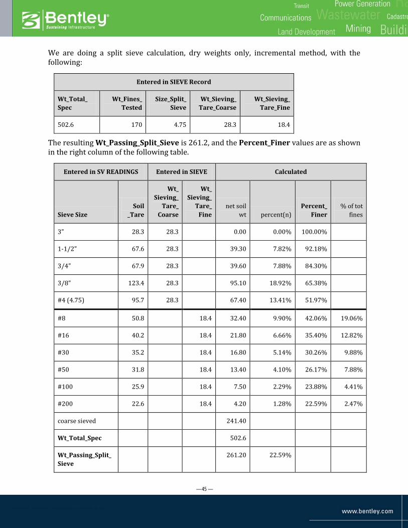
We are doing a split sieve calculation, dry weights only, incremental method, with the following:
Entered in SIEVE Record
Wt_Total_ Spec
Wt_Fines_ Tested
Size_Split_ Sieve
Wt_Sieving_ Tare_Coarse
Wt_Sieving_ Tare_Fine
502.6 170 4.75 28.3 18.4
The resulting Wt_Passing_Split_Sieve is 261.2, and the Percent_Finer values are as shown in the right column of the following table.
Entered in SV READINGS Entered in SIEVE Calculated
Sieve Size Soil
_Tare
Wt_ Sieving_
Tare_ Coarse
Wt_ Sieving_
Tare_ Fine
net soil wt percent(n)
Percent_Finer
% of tot fines
3" 28.3 28.3 0.00 0.00% 100.00%
1-1/2" 67.6 28.3 39.30 7.82% 92.18%
3/4" 67.9 28.3 39.60 7.88% 84.30%
3/8" 123.4 28.3 95.10 18.92% 65.38%
#4 (4.75) 95.7 28.3 67.40 13.41% 51.97%
#8 50.8 18.4 32.40 9.90% 42.06% 19.06%
#16 40.2 18.4 21.80 6.66% 35.40% 12.82%
#30 35.2 18.4 16.80 5.14% 30.26% 9.88%
#50 31.8 18.4 13.40 4.10% 26.17% 7.88%
#100 25.9 18.4 7.50 2.29% 23.88% 4.41%
#200 22.6 18.4 4.20 1.28% 22.59% 2.47%
coarse sieved 241.40
Wt_Total_Spec 502.6
Wt_Passing_Split_Sieve
261.20 22.59%

— 46 —
Setting up a Sieve Readings List in DATA DESIGN
You can define a set of sieve sizes in mm, and corresponding user-friendly names, that will automatically be inserted in the SV READINGS table when you add a SIEVE record. To see how this feature works, do the following:
1. Go to DATA DESIGN Readings Lists. Notice that a table of sieve sizes appears, with a Reading column for the measurement in mm, and a Name column for a corresponding user-friendly name for each.
2. Click the drop-down arrow on the object selector, and notice that there are multiple lists in the current library.
You can edit an existing list, and add lists to or delete them from the library, comparably to working with library tables. In particular:
ο Entering data in the bottom row (preceded by an asterisk) adds the record.
ο Highlighting a row and pressing Delete removes a record.
ο File Copy Page creates a new list that is a duplicate of the current list, but with a new name. This enables you to make a copy of a list, then edit the copy,

— 47 —
without altering the original.
ο File Delete Current Page removes the current list permanently from the library.
3. Go to DATA DESIGN Project Database, and open the current database. Select SV READINGS in the object selector.
4. Highlight the Reading field (captioned as “Sieve Size” in INPUT) in the Fields list at left.
5. Click the drop-down arrow to the right of the Default List property. Notice that all the sieve readings lists that exist in DATA DESIGN Readings are available for selection.
To configure the database to use a particular sieve readings list to populate the child records for a new SIEVE record, you do so here, namely, in the Default List property for the Reading field in the SV READINGS table in DATA DESIGN Project Database. Note that this does not change the set of readings attached to any existing SIEVE record, only ones you create after setting up the association the readings list.
6. Go to INPUT Sieve (INPUT Lab Testing Sieve in some databases). Create a new row in the bottom of the upper (parent) table grid by clicking in the Depth cell in the bottom row (the one with an asterisk to the left) and selecting a currently unused Depth value. Click another cell in the row, and notice that a new set of records, pre-populated with Sieve Size and Name values, appears in the lower (SV READINGS) grid.

— 48 —
7. Highlight the new row in the upper grid, and press Delete to remove it.
Setting up Individual Tares for Sieves
Some labs will place the entire sieve with the material retained onto the scale. In this case the tare for each sieve will be different and the tare weights in the parent grid do not apply.
To input tare weights for each individual sieve in the test, you must add a numeric field called Wt_Sieve_Tare to the SV READINGS table. Note that this exact field name must be created, although you can caption it differently. If the Wt_Sieve_Tare field exists and all the data rows in SV READINGS for the current parent record have values in this field, the program will ignore the sieving tare values in the parent SIEVE record and use the individual tare values in the child. However, if some of the child records containing Soil_Tare values have Wt_Sieve_Tare values and others do not, you will receive an error message to fill in Wt_Sieve_Tare for all the data rows or leave them all blank (and use the sieving tares in the parent grid).

— 49 —
Some Typical Reports
GRAIN SIZE (Grain Size Distribution) graph
The graph in the upper portion plots the results of sieve and hydrometer tests performed on soil specimens. These are known as grain size or particle size curves. For the sieve analysis, the percent finer is plotted for each sieve size opening (in US units on the upper scale and mm on the lower). For the hydrometer analysis, the percent fine is plotted for each grain size.

— 50 —
The lower portion provides an analysis of the sieve and hydrometer tests, combined with Atterberg data (including classifications derived from the Atterberg data). Percentages of gravel, sand, silt, and clay-size particles have been calculated, as well as D100, D60, D30 and D10 particle sizes. The D100 is the largest particle size recorded, the D60 is the particle size corresponding to 60% finer by dry weight, D30 is the particle size corresponding to 30 percent finer by dry weight, and D10 is the particle size corresponding to 10% finer by dry weight. Using the particle size dimension data, the coefficient of uniformity and coefficient of curvature can be calculated.
Cu = D60 / D10
Cc = (D30)2 / D10 x D60
These two parameters are used in the USCS to determine whether a soil is well-graded (many different particle sizes) or poorly graded (many particles of about the same size).
If the sieve and the hydrometer tests are performed correctly, the portion of the grain size curve from the sieve analysis should flow smoothly into the portion of the curve from the hydrometer analysis. A large and abrupt jump in the grain size curve from the sieve to the hydrometer test indicates errors in the lab testing procedure. [Source: Soil Testing Manual: Procedures, Classification Data and Sampling by Robert Day, McGraw Hill, 2000.]
Notice that each curve is for one specimen, that is, one PointID-Depth combination. Each page in the report contains a maximum of five curves, each identified under ‘Specimen Identification’ (including legend symbols) at the bottom. The specimens presented as curves and table data on each page are not necessarily grouped together functionally; after each page fills up with five specimens, a new page is started. If you want to limit the results to particular PointID-Depth combinations, you can do this at output time in the Borehole ID, Depth field. Alternately, or in addition, you can specify the sort order of specimens using the Sort 1 and Sort 2 fields.
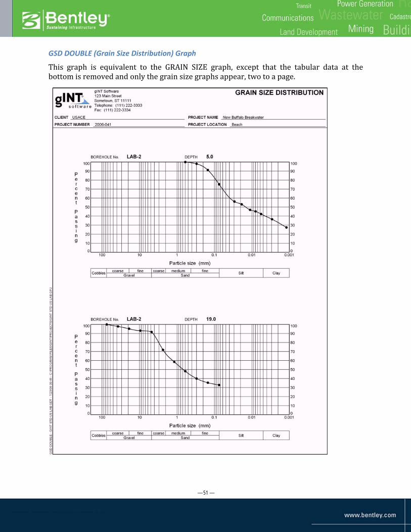
— 51 —
GSD DOUBLE (Grain Size Distribution) Graph
This graph is equivalent to the GRAIN SIZE graph, except that the tabular data at the bottom is removed and only the grain size graphs appear, two to a page.

— 52 —
FINES CONTENT (Fines Content Frequency) Histogram
This histogram provides a frequency distribution of the various fines content percentages for specimens spread over some range of boreholes. The data for all specimens is condensed onto a single report page.

— 53 —
While you can obtain the histogram for specimens across the entire project or for selected boreholes or specimens, the most useful application is to set up a range filter to select samples in a particular lithology layer across the project. To accomplish this, you enter something similar to the following in the Range Filter query builder fields at the lower right of the OUTPUT tab:
Field Value
Range Top Field [LITHOLOGY].[Depth]
Range Bottom Field [LITHOLOGY].[Bottom]
Include Top/Bottom Top
Criterion Field [LITHOLOGY].[Graphic]
Criteria ='CL'
Or ='CL-CH'
Or ='CLG'
Or ='CL-ML'
Or ='CLS'
In this case, specimens with a depth within the depth range of a lithology layer containing clay soils (CL, CL-CH, CLG, CL-ML or CLS) will be included in the histogram, and all other specimens will be excluded.
Other Graphs/Reports
SV READINGS table data is used in other standard graphs and reports in the following ways:
• In the LAB SUMMARY graphic table or text table, the maximum sieve size and percentage less than the #200 sieve are reported for each specimen (PointID-Depth combination).
• In the INDEX PROPS graph, percentage of fines is plotted against depth for each boring (PointID).
• In the GEOTECH BH PLOTS log, the plot-vs-depth column at right in this log report graphs, among other things, fines content percentage (curve with hollow square markers).
Custom reports can reference or use values from SIEVE and SV READINGS as the user desires.

— 54 —
Hydrometer Analysis
Background
The particle distribution for fines (silt and clay size particles finer than the #200 sieve) is determined by a sedimentation process. A hydrometer is used to obtain the necessary data during the sedimentation process. The hydrometer test is based on Stoke’s law, which relates the diameter of a single sphere to the time required for the sphere to fall a certain distance in a liquid of known viscosity. The idea for the hydrometer analysis is that a larger, and hence heavier, soil particle will fall faster through distilled water than a smaller, and hence lighter, soil particle. The test procedure is approximate because many fine soil particles are not spheres, but rather have a plate-like shape. Thus, while the sieve analysis uses the size of a square sieve opening to define particle size, the hydrometer analysis uses the diameter of an equivalent sphere as the definition of particle size.
Hydrometer testing is performed in accordance with ASTM D422. The soil specimen is first wet-sieved (to remove particles too large for hydrometer analysis) and washed with distilled water. Water is evaporated from the soil-water solution if necessary to bring the total volume to less than 1000 mL. A dispersing (defloculating) agent, typically 5 grams of sodium hexametaphosphate, is added, and the soil, water and dispersing agent are thoroughly mixed and allowed to soak overnight. This is to prevent the clay-sized particles from aggregating into flocs (clods) during the test. Remixing is performed, if needed. Then the slurry is added to a 1000-mL glass sedimentation cylinder, water added to the 1000 mL mark, and the cylinder closed with a rubber stopper and shaken for a minute. The cylinder is set down in a location free of vibration and other disturbances, and readings are taken at 1, 2, 5, 15, 30, 60, 250 and 1440 minutes. About 20-25 seconds before each hydrometer reading is due, the hydrometer is carefully inserted into the solution, and read by determining the number on the stem of the hydrometer that corresponds to the water meniscus. Then the hydrometer is removed and cleaned. A temperature reading is also taken. Two types of hydrometers are supported in ASTM D422: the 151H is graduated to read in specific gravity, the 152H in grams per liter of suspension. The latter is more popular since it records the actual mass of soil particles and dispersant in solution. (Day, 2001, p 54).
Data Entry
The Hydrometer tab is for data entry in the HYDROMETER and HYD READINGS tables. One HYDROMETER table record can be created for each borehole-depth combination present in the LAB SPECIMEN table and holds data that applies to all of its child (HYD READINGS) records. Multiple HYD READINGS records are created for a HYDROMETER record, and each holds data from one hydrometer reading obtained for the parent’s borehole-depth combination.
If only final results (particle size and percent finer for each reading event) are to be input, all of the upper grid (HYDROMETER) record information (except Depth) can be left blank. Otherwise, all fields in the row are required except for Calibration 2nd Order Term.

— 55 —
Typically the calibration field values (Type, Temperature Units Calibration, Calibration Intercept and Calibration Slope) are entered by selecting a value in the HydrometerID selection list, which selects a hydrometer that you have previously calibrated and defined in the HYDROMETER CALIBRATIONS library table, as described in “Setting up Hydrometer Calibrations in the Library Table” on page 57.
Important Note: Do not use the ‘US_DEMO’ hydrometer selection in HydrometerID. It is provided only as an example, and bears no relationship to the actual composite corrections you need to use for actual hydrometers in your lab. Calibrate your own hydrometer or hydrometers, define it/them in HYDROMETER CALIBRATIONS, and specify it in HYDROMETER table rows in HydrometerID.
For each reading event, create one child record with the Time, Hydrometer Reading, and Temperature of each reading. After all reading events are entered, click the Save icon, and the Particle Size and Percent Finer values are calculated automatically. Note that if a temperature field is blank, the value from the record above it is used.
HYDROMETER table fields
Field Name Lookup Description
PointID In combination with Depth, specifies the parent LAB SPECIMEN record. (Specified in the object selector)
Depth In combination with PointID, specifies the parent LAB SPECIMEN record.
Wt_Dry_ Specimen
In grams. This is the net (just soil, no tare) weight in grams of the specimen that was actually used in the hydrometer test.
Percent_Of_ Total
Percent of the total original specimen that is represented by the hydrometer test specimen, e.g., if hydrometer specimen split on #40 sieve, this field contains the % passing the #40 sieve.
Specific_ Gravity
This specific gravity is that of the hydrometer specimen and is not necessarily the same as the specific gravity given in the LAB SPECIMEN or FINE SG tables.
Temperature_ Units_Test
Lookup!lab temp units
The temperature units used in the test readings. This may or may not be the same as the calibration units.
HydrometerID Libtbl! hydrometer calibrations
Selects a set of calibration values for one hydrometer from the HYDROMETER CALIBRATIONS library table. On supplying a HydrometerID and saving, the program will copy the calibration parameters from the specified library table row to the corresponding fields in the current HYDROMETER row (if you leave all four of the calibration fields empty). If you specify a HydrometerID but also supply values in some of the calibration parameter fields, the program will use the library table values for the empty fields only.
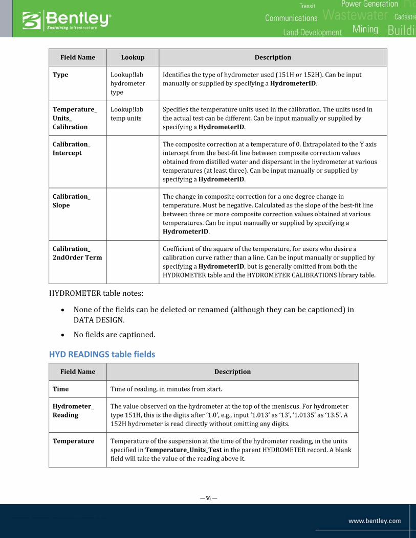
— 56 —
Field Name Lookup Description
Type Lookup!lab hydrometer type
Identifies the type of hydrometer used (151H or 152H). Can be input manually or supplied by specifying a HydrometerID.
Temperature_ Units_ Calibration
Lookup!lab temp units
Specifies the temperature units used in the calibration. The units used in the actual test can be different. Can be input manually or supplied by specifying a HydrometerID.
Calibration_ Intercept
The composite correction at a temperature of 0. Extrapolated to the Y axis intercept from the best-fit line between composite correction values obtained from distilled water and dispersant in the hydrometer at various temperatures (at least three). Can be input manually or supplied by specifying a HydrometerID.
Calibration_ Slope
The change in composite correction for a one degree change in temperature. Must be negative. Calculated as the slope of the best-fit line between three or more composite correction values obtained at various temperatures. Can be input manually or supplied by specifying a HydrometerID.
Calibration_ 2ndOrder Term
Coefficient of the square of the temperature, for users who desire a calibration curve rather than a line. Can be input manually or supplied by specifying a HydrometerID, but is generally omitted from both the HYDROMETER table and the HYDROMETER CALIBRATIONS library table.
HYDROMETER table notes:
• None of the fields can be deleted or renamed (although they can be captioned) in DATA DESIGN.
• No fields are captioned.
HYD READINGS table fields
Field Name Description
Time Time of reading, in minutes from start.
Hydrometer_ Reading
The value observed on the hydrometer at the top of the meniscus. For hydrometer type 151H, this is the digits after ‘1.0’, e.g., input ‘1.013’ as ‘13’, ‘1.0135’ as ‘13.5’. A 152H hydrometer is read directly without omitting any digits.
Temperature Temperature of the suspension at the time of the hydrometer reading, in the units specified in Temperature_Units_Test in the parent HYDROMETER record. A blank field will take the value of the reading above it.
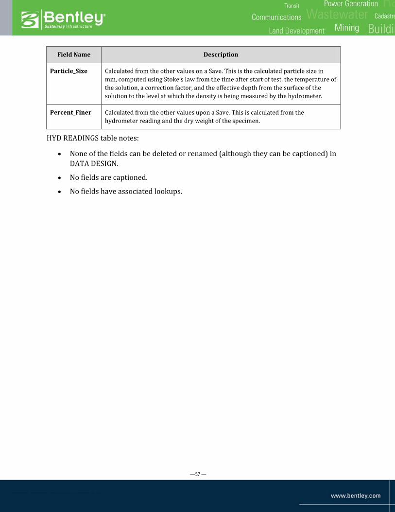
— 57 —
Field Name Description
Particle_Size Calculated from the other values on a Save. This is the calculated particle size in mm, computed using Stoke’s law from the time after start of test, the temperature of the solution, a correction factor, and the effective depth from the surface of the solution to the level at which the density is being measured by the hydrometer.
Percent_Finer Calculated from the other values upon a Save. This is calculated from the hydrometer reading and the dry weight of the specimen.
HYD READINGS table notes:
• None of the fields can be deleted or renamed (although they can be captioned) in DATA DESIGN.
• No fields are captioned.
• No fields have associated lookups.

— 58 —
Setting up Hydrometer Calibrations in the Library Table
The composite correction (see ASTM D422) is a value subtracted from the specific gravity reading recorded on the hydrometer at a particular time. Composite correction is used to adjust each hydrometer reading downwards to reflect the effect of dispersant specific gravity, meniscus height, and temperature-induced error. The correction value is temperature dependent, and so is obtained from an (almost always) linear equation that plots the offset in specific gravity against the temperature of the solution. From the solution temperature at the time of the reading, the composite correction to deduct at that temperature is derived from the equation.
In addition to correcting for temperature, the composite correction line or curve compensates for the following:
• The change in specific gravity due to adding dispersant.
• The height of the meniscus. Since the hydrometer reading is supposed to be taken at the bottom of the meniscus, but this cannot be seen through a soil suspension, readings are taken at the top of the meniscus and the composite correction compensates for the distance between meniscus top and bottom.

— 59 —
Each hydrometer/dispersing agent combination has its own correction line (or curve). This is obtained experimentally as described in ASTM D422, by taking hydrometer readings at various temperatures for the specified hydrometer and dispersing agent solution, and plotting these points on a graph. A best-fit line between the experimental points is drawn, and the slope and Y-intercept of this line determined, as shown:
The slope and intercept specified in Calibration_Slope and Calibration_Intercept are used to calculate the composite correction value for a given temperature.
Composite_correction is calculated as follows:
composite_correction = (Calibration_Slope x Temperature) + Calibration_Intercept
where: Calibration_Slope, Temperature, and Calibration_Intercept are all in the same temperature units (Celsius or Fahrenheit)
Example:
Entered in HYDROMETER (or library table)
Entered in HYD READINGS
Calculated
Calibration_ Intercept
Calibration_ Slope
Temperature composite correction
13.15383 -0.38163 22 4.76
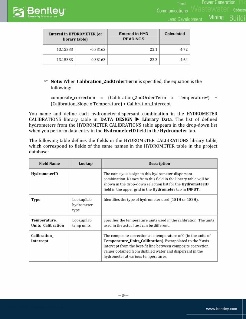
— 60 —
Entered in HYDROMETER (or library table)
Entered in HYD READINGS
Calculated
13.15383 -0.38163 22.1 4.72
13.15383 -0.38163 22.3 4.64
Note: When Calibration_2ndOrderTerm is specified, the equation is the following:
composite_correction = (Calibration_2ndOrderTerm x Temperature2) + (Calibration_Slope x Temperature) + Calibration_Intercept
You name and define each hydrometer-dispersant combination in the HYDROMETER CALIBRATIONS library table in DATA DESIGN Library Data. The list of defined hydrometers from the HYDROMETER CALIBRATIONS table appears in the drop-down list when you perform data entry in the HydrometerID field in the Hydrometer tab.
The following table defines the fields in the HYDROMETER CALIBRATIONS library table, which correspond to fields of the same names in the HYDROMETER table in the project database:
Field Name Lookup Description
HydrometerID The name you assign to this hydrometer-dispersant combination. Names from this field in the library table will be shown in the drop-down selection list for the HydrometerID field in the upper grid in the Hydrometer tab in INPUT.
Type Lookup!lab hydrometer type
Identifies the type of hydrometer used (151H or 152H).
Temperature_ Units_ Calibration
Lookup!lab temp units
Specifies the temperature units used in the calibration. The units used in the actual test can be different.
Calibration_ Intercept
The composite correction at a temperature of 0 (in the units of Temperature_Units_Calibration). Extrapolated to the Y axis intercept from the best-fit line between composite correction values obtained from distilled water and dispersant in the hydrometer at various temperatures.

— 61 —
Field Name Lookup Description
Calibration_ Slope The change in composite correction for a one degree change in temperature. Must be negative. Calculated as the slope of the best-fit line between composite correction values obtained at various temperatures.
Note that the hydrometer calibrations may have a 0 value for the intercept and slope. The reason for this is that some users enter corrected hydrometer readings. In this case there is no calibration correction necessary, and zero is specified for both the slope and the intercept.
Calibration_ 2ndOrder Term
Coefficient of the square of the temperature, for the rare case of users who desire a calibration curve rather than a line. Generally omitted from both the HYDROMETER table and the HYDROMETER CALIBRATIONS library table.
Notes Field for your internal documentation, not used in the program.
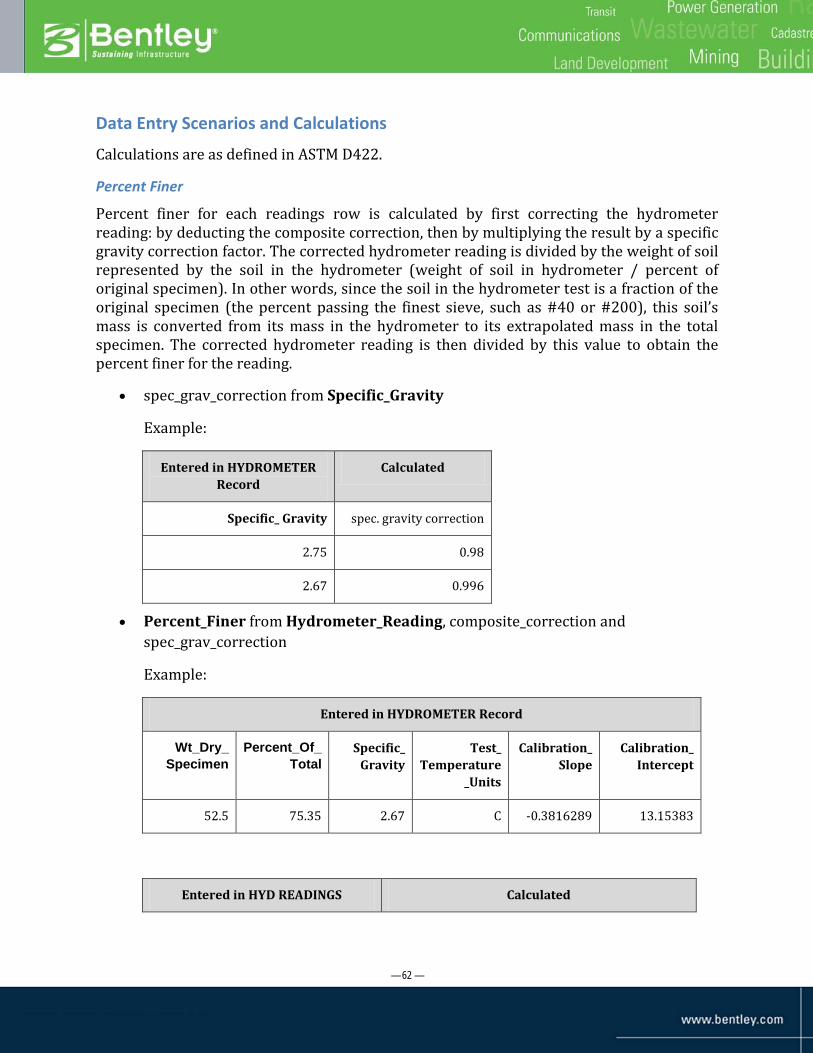
— 62 —
Data Entry Scenarios and Calculations
Calculations are as defined in ASTM D422.
Percent Finer
Percent finer for each readings row is calculated by first correcting the hydrometer reading: by deducting the composite correction, then by multiplying the result by a specific gravity correction factor. The corrected hydrometer reading is divided by the weight of soil represented by the soil in the hydrometer (weight of soil in hydrometer / percent of original specimen). In other words, since the soil in the hydrometer test is a fraction of the original specimen (the percent passing the finest sieve, such as #40 or #200), this soil’s mass is converted from its mass in the hydrometer to its extrapolated mass in the total specimen. The corrected hydrometer reading is then divided by this value to obtain the percent finer for the reading.
• spec_grav_correction from Specific_Gravity
Example:
Entered in HYDROMETER Record
Calculated
Specific_ Gravity spec. gravity correction
2.75 0.98
2.67 0.996
• Percent_Finer from Hydrometer_Reading, composite_correction and spec_grav_correction
Example:
Entered in HYDROMETER Record
Wt_Dry_ Specimen
Percent_Of_ Total
Specific_ Gravity
Test_ Temperature
_Units
Calibration_ Slope
Calibration_ Intercept
52.5 75.35 2.67 C -0.3816289 13.15383
Entered in HYD READINGS Calculated
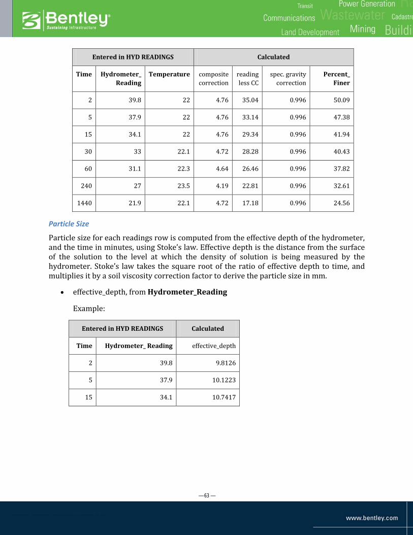
— 63 —
Entered in HYD READINGS Calculated
Time Hydrometer_ Reading
Temperature composite correction
reading less CC
spec. gravity correction
Percent_ Finer
2 39.8 22 4.76 35.04 0.996 50.09
5 37.9 22 4.76 33.14 0.996 47.38
15 34.1 22 4.76 29.34 0.996 41.94
30 33 22.1 4.72 28.28 0.996 40.43
60 31.1 22.3 4.64 26.46 0.996 37.82
240 27 23.5 4.19 22.81 0.996 32.61
1440 21.9 22.1 4.72 17.18 0.996 24.56
Particle Size
Particle size for each readings row is computed from the effective depth of the hydrometer, and the time in minutes, using Stoke’s law. Effective depth is the distance from the surface of the solution to the level at which the density of solution is being measured by the hydrometer. Stoke’s law takes the square root of the ratio of effective depth to time, and multiplies it by a soil viscosity correction factor to derive the particle size in mm.
• effective_depth, from Hydrometer_Reading
Example:
Entered in HYD READINGS Calculated
Time Hydrometer_ Reading effective_depth
2 39.8 9.8126
5 37.9 10.1223
15 34.1 10.7417

— 64 —
• viscosity_correction, from Temperature and Specific_Gravity
Example:
Entered in HYDROMETER
Entered in HYD READINGS
Calculated
Specific_ Gravity Temperature viscosity correction factor
2.67 22.1 0.013205
2.67 22.3 0.013175
• Particle_Size, from Time, effective_depth, and viscosity_correction
Example:
Entered in HYD READINGS Calculated
Time Hydrometer_Reading
Temp-erature
viscosity correction factor
effective depth
Particle_ Size
2 39.8 22 0.01322 9.8126 0.029283
5 37.9 22 0.01322 10.1223 0.01881
15 34.1 22 0.01322 10.7417 0.011187
Some Typical Reports
The reports and graphs for hydrometer analysis are the same as for sieve analysis, namely the GRAIN SIZE, GSD DOUBLE, and FINES CONTENT graph reports, and miscellaneous appearances of the data in other reports. Refer to the “Reporting” section in the “Sieve Analysis” chapter.

— 65 —
Fine Specific Gravity
Background
The definition of specific gravity is the ratio of the weight in air of a given volume of a material at a stated temperature to the weight in air of an equal volume of distilled water at a stated temperature. The specific gravity test is made on that portion of soil which passes the No. 4 (4.75 mm) sieve. The test is performed using a pyknometer, also called specific gravity bottle. This is a glass flask with a close-fitting ground glass stopper with a capillary tube through it so that air bubbles may escape from the apparatus. A vacuum pump is typically used to assist in the removal of air bubbles. The flask is weighed with distilled water up to a specific mark, and then with distilled water/soil suspension (with air bubbles removed) up to the same mark. From the two weights, and the weight of dry soil that has been added, the specific gravity of the soil is calculated. Adjustment is also made for the temperature at which the readings are performed, if this deviates from 20 degrees C. The procedure is specified in ASTM D854.
Data Entry
The Fine SG tab is for data entry in the FINE SG and FINE SG READINGS tables. One FINE SG table record can be created for each borehole-depth combination present in the LAB SPECIMEN table. Multiple FINE SG READINGS records can be created for a FINE SG record, and each holds data from one specific gravity reading obtained for the parent’s borehole-depth combination.
The Fine SG tab provides the means to calculate the specific gravity of the fines fraction of a soil specimen from multiple readings. The specific gravity values of the readings are computed individually, then averaged and used to populate the Specific_Gravity field in the parent FINE SG record. However, this value is not reported in any standard reports or used in calculations elsewhere in lab testing.
The Readings_Temperature_Units (Fahrenheit or Centigrade) field in the FINE SG table is required. Also, for any readings row created in FINE SG READINGS, all fields are required except Specific_Gravity (which is calculated from the other fields).
FINE SG table fields
Field Name Lookup Description
PointID In combination with Depth, specifies the parent LAB SPECIMEN record. (Specified in the object selector)
Depth In combination with PointID, specifies the parent LAB SPECIMEN record.
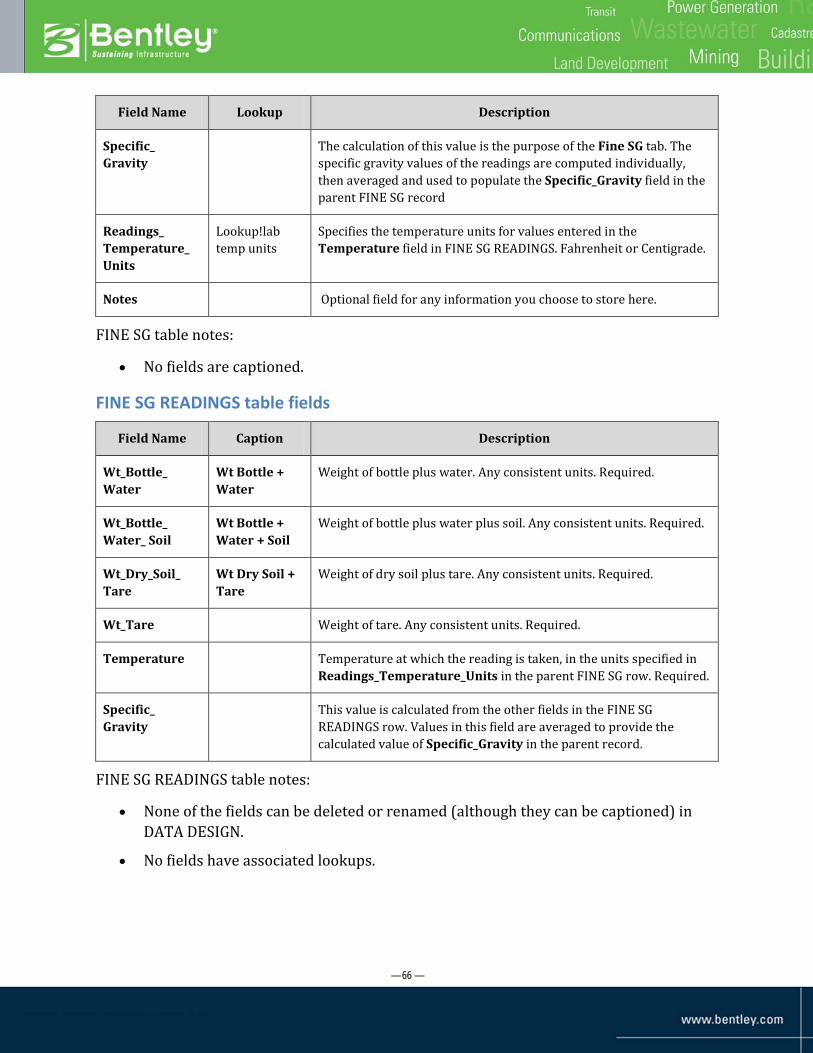
— 66 —
Field Name Lookup Description
Specific_ Gravity
The calculation of this value is the purpose of the Fine SG tab. The specific gravity values of the readings are computed individually, then averaged and used to populate the Specific_Gravity field in the parent FINE SG record
Readings_ Temperature_ Units
Lookup!lab temp units
Specifies the temperature units for values entered in the Temperature field in FINE SG READINGS. Fahrenheit or Centigrade.
Notes Optional field for any information you choose to store here.
FINE SG table notes:
• No fields are captioned.
FINE SG READINGS table fields
Field Name Caption Description
Wt_Bottle_ Water
Wt Bottle + Water
Weight of bottle plus water. Any consistent units. Required.
Wt_Bottle_ Water_ Soil
Wt Bottle + Water + Soil
Weight of bottle plus water plus soil. Any consistent units. Required.
Wt_Dry_Soil_ Tare
Wt Dry Soil + Tare
Weight of dry soil plus tare. Any consistent units. Required.
Wt_Tare Weight of tare. Any consistent units. Required.
Temperature
Temperature at which the reading is taken, in the units specified in Readings_Temperature_Units in the parent FINE SG row. Required.
Specific_ Gravity
This value is calculated from the other fields in the FINE SG READINGS row. Values in this field are averaged to provide the calculated value of Specific_Gravity in the parent record.
FINE SG READINGS table notes:
• None of the fields can be deleted or renamed (although they can be captioned) in DATA DESIGN.
• No fields have associated lookups.
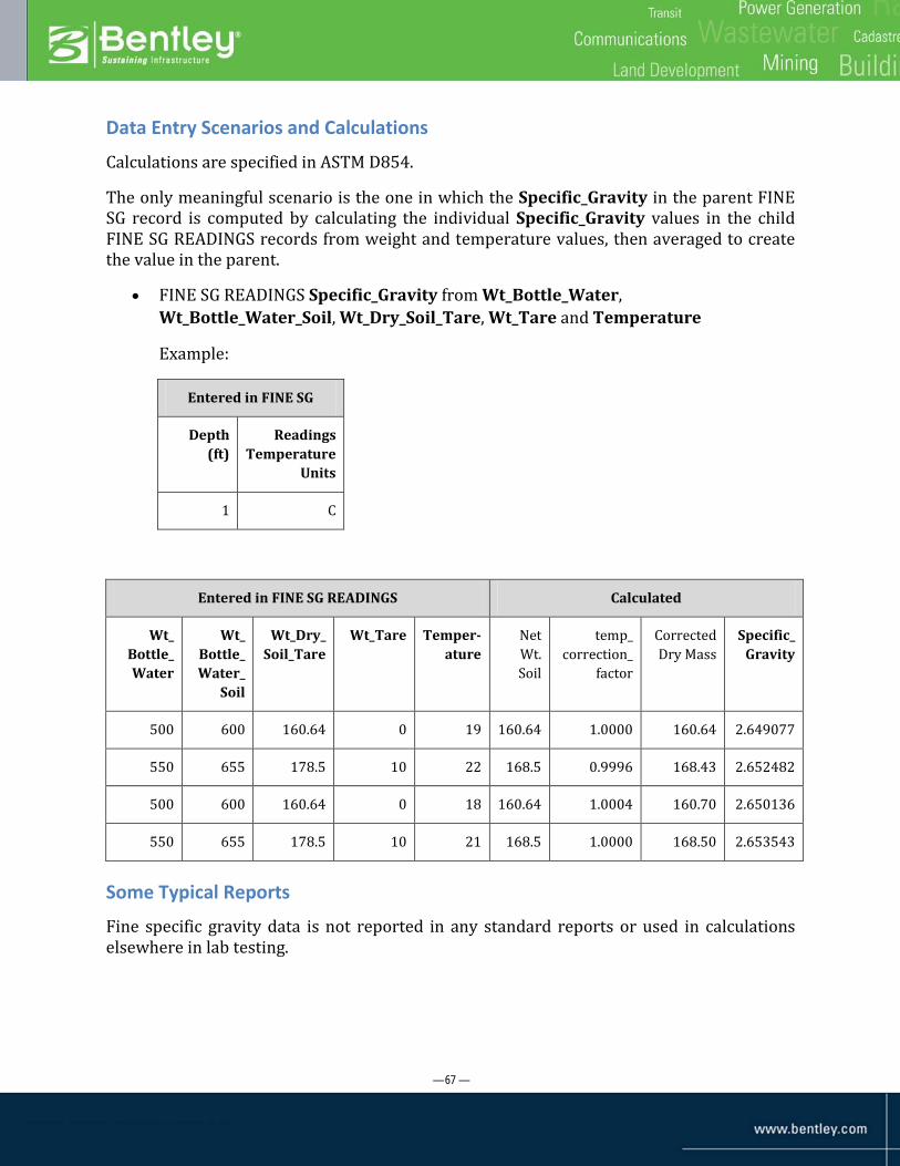
— 67 —
Data Entry Scenarios and Calculations
Calculations are specified in ASTM D854.
The only meaningful scenario is the one in which the Specific_Gravity in the parent FINE SG record is computed by calculating the individual Specific_Gravity values in the child FINE SG READINGS records from weight and temperature values, then averaged to create the value in the parent.
• FINE SG READINGS Specific_Gravity from Wt_Bottle_Water, Wt_Bottle_Water_Soil, Wt_Dry_Soil_Tare, Wt_Tare and Temperature
Example:
Entered in FINE SG
Depth (ft)
Readings Temperature
Units
1 C
Entered in FINE SG READINGS Calculated
Wt_ Bottle_ Water
Wt_ Bottle_ Water_
Soil
Wt_Dry_ Soil_Tare
Wt_Tare Temper-ature
Net Wt. Soil
temp_ correction_
factor
Corrected Dry Mass
Specific_ Gravity
500 600 160.64 0 19 160.64 1.0000 160.64 2.649077
550 655 178.5 10 22 168.5 0.9996 168.43 2.652482
500 600 160.64 0 18 160.64 1.0004 160.70 2.650136
550 655 178.5 10 21 168.5 1.0000 168.50 2.653543
Some Typical Reports
Fine specific gravity data is not reported in any standard reports or used in calculations elsewhere in lab testing.

— 68 —
Compaction
Background
Compaction is the process of increasing the bulk density of a soil or aggregate by driving out air. For any soil, for a given amount of compactive effort, the density obtained depends on the moisture content. At very high moisture contents, the maximum dry density is achieved when the soil is compacted to nearly saturation, where (almost) all the air is driven out. At low moisture contents, the soil particles interfere with each other; addition of some moisture will allow greater bulk densities, with a peak density where this effect begins to be counteracted by the saturation of the soil.
The result of soil compaction is measured by determining the bulk density of the compacted soil and comparing it to a maximum density obtained from a compaction test, to determine the relative compaction.
Lab testing for compaction consists of compacting a soil at a known water content into a mold of specific dimensions using a certain compaction energy. The procedure is repeated for various water contents to establish the compaction curve. The most common test procedures for compaction are the modified Proctor (ASTM D1557) and the standard Proctor (ASTM D698). The latter uses a lower compaction energy, and is used less frequently. In either case, the test procedure is to prepare soil at a certain water content, compact the soil into the molds, and then, by recording the mass of soil within the mold, obtain the wet density of the compacted soil. By knowing the water content of the compacted soil, the dry density can be calculated.
This compaction procedure is repeated for the soil at different water contents, and then the dry density versus water content is plotted on a graph to obtain the compaction curve. The peak point of the compaction curve is known as the laboratory maximum dry density. The water content corresponding to the peak point of the lab compaction curve is known as the optimum moisture content. (Day, 2001, p 293).
Data Entry
The Compaction tab is for data entry in the COMPACTION and COMP READINGS tables. One COMPACTION table record can be created for each borehole-depth combination present in the LAB SPECIMEN table and holds data that applies to all of its child (COMP READINGS) records. Multiple COMP READINGS records are created for a COMPACTION record, and each holds data from one compaction test reading obtained for the parent’s borehole-depth combination.
The COMPACTION record is for entry of mold weight and volume fields utilized in the calculation of Wet_Density and Dry_Density values in its child COMP READINGS records. It also has certain fields whose values are reported on compaction graphs (Max_Dry_Density, Opt_Moisture_Content, and Method). However, with one exception (optional automatic calculation of Max_Dry_Density and Opt_Moisture_Content,
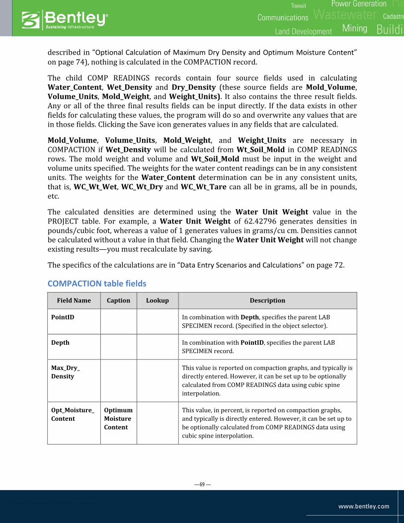
— 69 —
described in “Optional Calculation of Maximum Dry Density and Optimum Moisture Content” on page 74), nothing is calculated in the COMPACTION record.
The child COMP READINGS records contain four source fields used in calculating Water_Content, Wet_Density and Dry_Density (these source fields are Mold_Volume, Volume_Units, Mold_Weight, and Weight_Units). It also contains the three result fields. Any or all of the three final results fields can be input directly. If the data exists in other fields for calculating these values, the program will do so and overwrite any values that are in those fields. Clicking the Save icon generates values in any fields that are calculated.
Mold_Volume, Volume_Units, Mold_Weight, and Weight_Units are necessary in COMPACTION if Wet_Density will be calculated from Wt_Soil_Mold in COMP READINGS rows. The mold weight and volume and Wt_Soil_Mold must be input in the weight and volume units specified. The weights for the water content readings can be in any consistent units. The weights for the Water_Content determination can be in any consistent units, that is, WC_Wt_Wet, WC_Wt_Dry and WC_Wt_Tare can all be in grams, all be in pounds, etc.
The calculated densities are determined using the Water Unit Weight value in the PROJECT table. For example, a Water Unit Weight of 62.42796 generates densities in pounds/cubic foot, whereas a value of 1 generates values in grams/cu cm. Densities cannot be calculated without a value in that field. Changing the Water Unit Weight will not change existing results—you must recalculate by saving.
The specifics of the calculations are in “Data Entry Scenarios and Calculations” on page 72.
COMPACTION table fields
Field Name Caption Lookup Description
PointID In combination with Depth, specifies the parent LAB SPECIMEN record. (Specified in the object selector).
Depth In combination with PointID, specifies the parent LAB SPECIMEN record.
Max_Dry_ Density
This value is reported on compaction graphs, and typically is directly entered. However, it can be set up to be optionally calculated from COMP READINGS data using cubic spine interpolation.
Opt_Moisture_Content
Optimum Moisture Content
This value, in percent, is reported on compaction graphs, and typically is directly entered. However, it can be set up to be optionally calculated from COMP READINGS data using cubic spine interpolation.

— 70 —
Field Name Caption Lookup Description
Method Libtbl! Compaction methods
Identifies the ASTM method used in performing the tests. This is an optional field used in reporting. Methods can be added to the COMPACTION METHODS library table, and subsequently used for lookup here. Note that while a number of fields are provided in the library table for future use, only Method (MethodID) and Description appear in lookups or reports.
Mold_Volume The volume of soil that the mold holds, in the volume units specified. This value must be entered if Wet_Density will be calculated from Wt_Soil_Mold in COMP READINGS rows.
Volume_Units Lookup! lab length units
Volume units used for entry of Mold_Volume and calculation of Wet_Density. Your entry (‘Ft’, ‘M’, ‘In’ etc. is interpreted as the corresponding cubic unit (cu ft, cu m, etc.)
Mold_Weight Tare weight of the mold. This value must be entered if Wet_Density will be calculated from Wt_Soil_Mold in COMP READINGS rows. It must be input in the weight units specified.
Weight_Units Lookup! lab weight units
Weight units used for entry of Mold_Weight and calculation of Wet_Density.
Notes Optional field not used in gINT standard lab testing reports, but available for your use in customized reports.

— 71 —
COMP READINGS table fields
Field Name Caption Description
Wt_Soil_Mold Wt Soil + Mold Weight of soil plus mold, in the units specified in the Mold_Weight field in the parent COMPACTION record.
WC_Wt_Wet Water Content Wet Wt+Tare
Weight of wet soil plus tare, in any consistent units. If omitted, Water_Content cannot be calculated.
WC_Wt_Dry Water Content Dry Wt+Tare
Weight of dry soil plus tare, in any consistent units. If omitted, Water_Content cannot be calculated.
WC_Wt_Tare Water Content Wt Tare
Weight of tare, in any consistent units. If omitted, Water_Content cannot be calculated.
Water_Content Also known as moisture content. In percent. Will be calculated if the data exists, or can be input directly.
Wet_Density Also known as wet unit weight or total unit weight. In units determined by the Water_Unit_Wt in PROJECT (62.42796 generates densities in pounds/cubic foot; 1 generates values in grams/cu cm). Will be calculated if the data exists, or can be input directly.
Dry_Density Also known as dry unit weight. In units determined by the Water_Unit_Wt field in PROJECT. Will be calculated if the data exists, or can be input directly.
COMP READINGS table notes:
• None of the fields can be deleted or renamed (although they can be captioned) in DATA DESIGN.
• There are no associated lookups
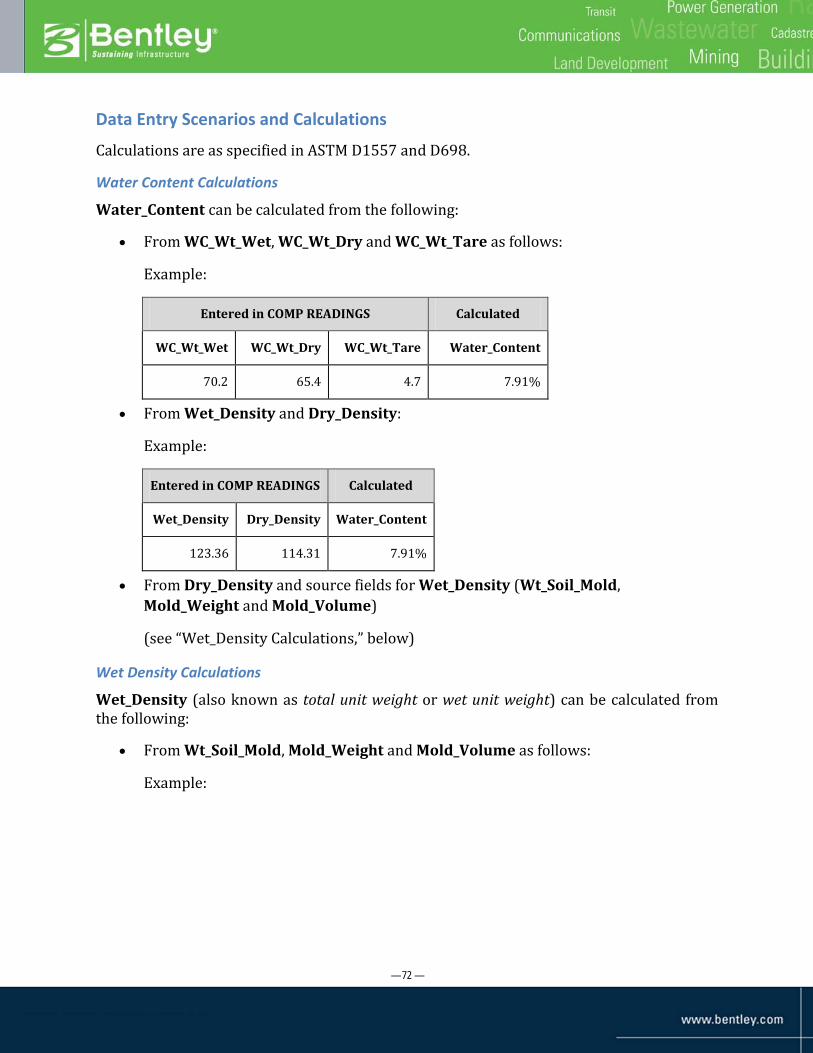
— 72 —
Data Entry Scenarios and Calculations
Calculations are as specified in ASTM D1557 and D698.
Water Content Calculations
Water_Content can be calculated from the following:
• From WC_Wt_Wet, WC_Wt_Dry and WC_Wt_Tare as follows:
Example:
Entered in COMP READINGS Calculated
WC_Wt_Wet WC_Wt_Dry WC_Wt_Tare Water_Content
70.2 65.4 4.7 7.91%
• From Wet_Density and Dry_Density:
Example:
Entered in COMP READINGS Calculated
Wet_Density Dry_Density Water_Content
123.36 114.31 7.91%
• From Dry_Density and source fields for Wet_Density (Wt_Soil_Mold, Mold_Weight and Mold_Volume)
(see “Wet_Density Calculations,” below)
Wet Density Calculations
Wet_Density (also known as total unit weight or wet unit weight) can be calculated from the following:
• From Wt_Soil_Mold, Mold_Weight and Mold_Volume as follows:
Example:

— 73 —
Entered in COMP READINGS
Entered in COMPACTION Calculated
Wt_Soil_Mold Mold_Weight Mold_Volume Volume Units Wet_Density
9.312 5.2 0.0333333 ft 123.36
• From Water_Content and Dry_Density
Example:
Entered in COMP READINGS Calculated
Dry_Density Water_Content Wet_Density
114.32 7.91% 123.36

— 74 —
Dry Density Calculations
Dry_Density (also known as dry unit weight) can be calculated from the following:
• From Water_Content and Wet_Density
Example:
Entered in COMP READINGS Calculated
Water_Content Wet_Density Dry_Density
31.32% 119.5 90.999
• From Water_Content and Wet_Density’s source fields (Wt_Soil_Mold, Mold_Weight and Mold_Volume)
(see “Wet Density Calculations,” above)
• From Wet_Density and Water_Content’s source fields (WC_Wt_Wet, WC_Wt_Dry and WC_Wt_Tare)
(see “Water Content Calculations,” above)
Optional Calculation of Maximum Dry Density and Optimum Moisture Content
By default, Max_Dry_Density and Opt_Moisture_Content (Optimium Water Content) fields in the COMPACTION table are not calculated by gINT from the data in the COMP READINGS table. This is because the computation methodology for these values is subject to user discretion, and gINT typically does not interpret data. However, you can add a checkbox field to COMPACTION that will cause the values entered in these two fields are to be calculated automatically when unchecked, using the cubic spline interpolation method of curve fitting. When checked, the default behavior is performed, namely, any values directly entered in these two fields are left intact following saves.
To set up optional calculation of Max_Dry_Density and Opt_Moisture_Content using cubic spline curve fitting, add the following field to the COMPACTION table in DATA DESIGN:
Name Type
Do Not Calc Max Opt Boolean
Be sure to create the field name exactly as written above.

— 75 —
After creating this field in DATA DESIGN, automatic calculation will occur in INPUT for COMPACTION rows that have this field unchecked. If the field doesn't exist, or it exists and is checked, the program will not perform the calculation, allowing you to insert whatever values you wish.
Disclaimer: Soil testing results, especially compaction tests, are open to interpretation. The automatic calculation methodology in gINT, if you activate it, may not be correct in the judgment of persons reviewing the work. It is your responsibility to double-check the results and make adjustments if you deem them necessary.
The calculation uses the Cubic Spline vs. Independent Axis (unadjusted) curve fitting method. Therefore, at least three points are required. If the fit fails for any reason, a message box will appear informing you that it could be not done. Note that this algorithm bases its results only on the data in the COMP READINGS table, and there is no accounting for rock correction or additional plot points that you may have added.
Note also that the calculated results using this method may or may not match the curve-fitting algorithm used to generate the curve(s) in the COMPACTION and COMPACTION (MULTIPLE CURVES) graphs in your library. Lab testing libraries created by gINT Software will typically specify this method, which appears as the ‘Cubic Spline vs Ind (unadjusted)’ selection in the Graph Line Option property of the Data Representation tab in the report properties for the graph in REPORT DESIGN. However, you may find it worthwhile to verify that this method is indeed specified in the report designs for your graphs, and change it if it isn’t.
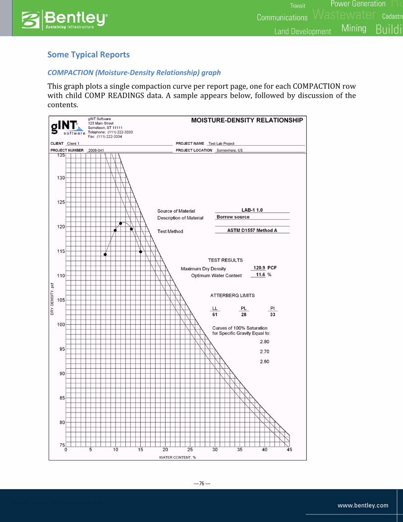
— 76 —
Some Typical Reports
COMPACTION (Moisture-Density Relationship) graph
This graph plots a single compaction curve per report page, one for each COMPACTION row with child COMP READINGS data. A sample appears below, followed by discussion of the contents.

— 77 —
In the graph, the points on the moisture-density curve are obtained from the Water_Content and Dry_Density values in the child COMP READINGS records for the point-depth combination indicated in the Source of Material field on the report. The curve interpolated between the points utilizes cubic spline curve fitting. The peak vertical value of the compaction curve is the laboratory maximum dry density, with the corresponding value on the X axis representing the optimum moisture content. The higher the maximum dry density, the more densely the soil can be compacted. Also, the moisture content value at this point is useful for grading contractors, who thereby know at approximately what water content the soil can be compacted most efficiently.
Along the right edge of the graph area are three zero air voids curves, also known as 100% saturation curves. These curves represent the relationship between water content and dry density for a condition of saturation for each of three specific gravities. The right side of the compaction curve typically parallels the zero air voids curves for many soil types.
To the right of the graph area, various data is reported, including the Atterberg indices for the point-depth combination (if this data is present in the Atterberg tab), the test method name (from the Method field in COMPACTION), and the entered or calculated Max_Dry_Density and Opt_Moisture_Content.
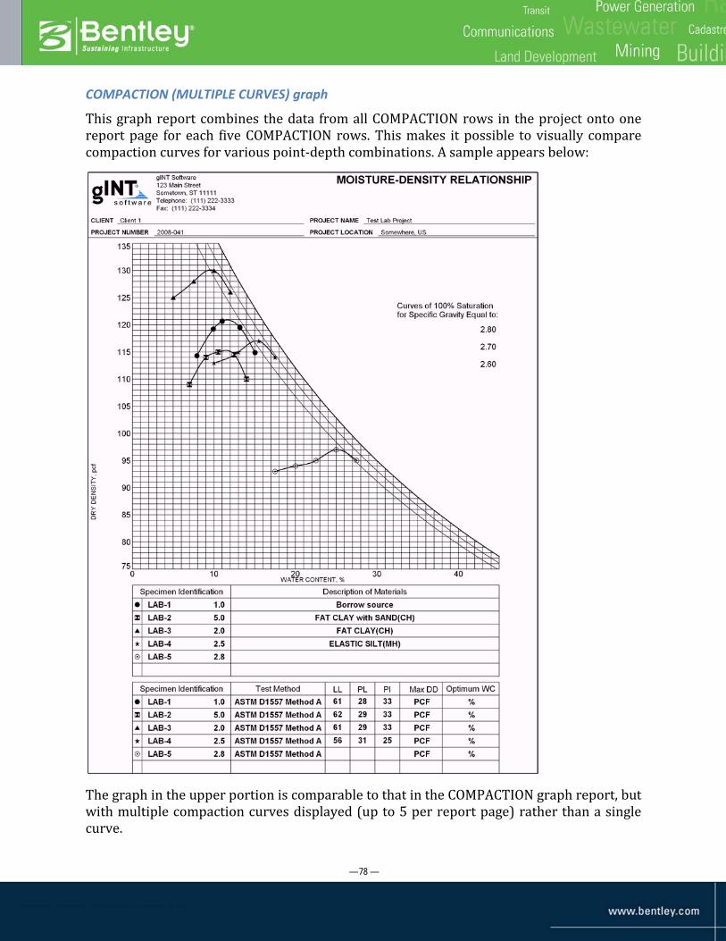
— 78 —
COMPACTION (MULTIPLE CURVES) graph
This graph report combines the data from all COMPACTION rows in the project onto one report page for each five COMPACTION rows. This makes it possible to visually compare compaction curves for various point-depth combinations. A sample appears below:
The graph in the upper portion is comparable to that in the COMPACTION graph report, but with multiple compaction curves displayed (up to 5 per report page) rather than a single curve.

— 79 —
The lower portion provides selected compaction data for each of the compaction curves, combined with the Atterberg data for the same point-depth (including classifications derived from the Atterberg data and fines content).
Notice that each curve is for one specimen, that is, one point-depth combination. Each page in the report contains a maximum of five curves, each identified under ‘Specimen Identification’ (including legend symbols) at the bottom. The specimens presented as curves and table data on each page are not necessarily grouped together functionally; after each page fills up with five specimens, a new page is started.

— 80 —
Unconfined Compression
Background
This test compresses a soil sample to measure its strength. The modifier "unconfined" contrasts this test to the triaxial shear test. This test method covers the determination of the unconfined compressive strength of cohesive soil in the intact, remolded, or reconstituted condition, using strain-controlled application of the axial load. It provides an approximate value of the strength of cohesive soils in terms of total stresses.
The test consists of applying a vertical compressive pressure to a cylinder of laterally unconfined cohesive soil. The unconfined compression test is also known as a simple compression test, and complies with ASTM D2166. An undisturbed sample of sufficient diameter is obtained, such as extruded from a sampler, and trimmed on the top and bottom to create a cylinder. The height, diameter and weight are measured, and water content and dry unit weight calculated. Then the soil cylinder is centered upright on a loading device capable of loading the soil specimen at a constant rate of strain. The device is adjusted so that the upper platen just makes contact with the top of the soil specimen, and the vertical deformation gauge is zeroed. A vertical load is applied to the specimen, with a strain rate as specified in ASTM D2166.
During the shearing of the soil specimen, two measurements are periodically recorded. One is the change in height of the soil specimen, called deflection in gINT. When divided by the initial height, deflection is converted to a value called axial strain, or simply strain, expressed as a percentage. The second measurement is vertical load or axial load, which is the force exerted on the surface exposed to that force. Load is converted to a value called stress, which measures the average amount of force exerted per unit area. Stress is expressed as the ratio of axial load to loaded surface area.
The shearing portion of the test continues until failure of the specimen, which means either than the specimen breaks apart, or 15% axial strain is reached. Then end-of-test moisture content measurements can be obtained, if desired, and overall strength and strain-at-failure values can be computed. The purpose of calculating moisture content and density is to determine whether there was a significant change between starting and final water content, which could indicate that the soil specimen dried out or bled water during testing.
(Day, 2001, p 251)

— 81 —
Axial load is measured mechanically or electronically. Load is measured mechanically by compressing a pre-calibrated load ring (also called a proving ring) and measuring the change in diameter, which translates to a value in units of force, such as psi.
Different load rings respond with greater or lesser amounts of diameter deflection to the same force, depending on ring material used, thickness, diameter and other factors, but the relationship between force and deflection are roughly linear.
Double load rings are also sometimes used, which consist of a stronger ring inside a weaker ring. The purpose of a double ring is to ensure that deflection in an appropriate range is measured, since selection of a single ring of the best deflection characteristics for the specimen can be guesswork. The weak outer ring measures weaker force; however if the force is beyond the range of what the outer ring can appropriately measure, the strong inner ring is encountered and compressed.
Data Entry
The Unconf Compr tab is for data entry in the UNCONF COMPR and UNC READINGS tables. One UNCONF COMPR table record can be created for each borehole-depth combination present in the LAB SPECIMEN table and holds data that applies to all of its child (UNC READINGS) records. Multiple UNC READINGS records are created for a UNCONF COMPR record, and each holds data from one unconfined compression test reading obtained for the parent’s borehole-depth combination.

— 82 —
The parent UNCONF COMPR record holds values that define the parameters of the test, such as load ring calibration data for the load ring used, the diameter and height of the specimen, and values for optional water content and wet/dry density computation. Also, the values of Strength and Strain_at_Failure in the parent row are computed as the Stress and Strain values from the child row with the maximum Stress value. Nothing is reported from UNCONF COMPR in the standard reports.
On a save, if a Load_Ring name as been supplied, gINT will copy the calibration parameters from the LOAD RINGS library table to the corresponding fields in the UNCONF COMPR record. Alternately the calibration values can be entered into UNCONF COMPR directly, and Load_Ring omitted. See “Setting up Load Ring Calibrations in the Library Table” on page 84.
In the readings table, the first record is assumed to be the initial condition before loading occurs. The initial load and deflection readings can be gauge readings which are not necessarily zero. The calculations use the differences between the readings and these initial readings.
UNCONF COMPR table fields
Field Name Lookup Description
PointID In combination with Depth, specifies the parent LAB SPECIMEN record. (Specified in the object selector).
Depth In combination with PointID, specifies the parent LAB SPECIMEN record.
Strength Calculated. Strength is the maximum Stress value for the child records in UNC READINGS for Strain values less than or equal to 15%. If the Strain values continue beyond 15% with increasing stress, the program interpolates the stress at 15%.
Strain_At_ Failure
Calculated. The Strain value in UNC READINGS for the maximum Stress value.
Load_Ring Libtbl! load rings
Specifies the name of a load ring calibration in the LOAD RINGS library table. If entered, on a save the program will copy the values from the row with this Ring_ID in the LOAD RINGS library table to Slope_Initial, Slope_Break and Slope_2ndary in the UNCONF COMPR record. See “Setting up Load Ring Calibrations in the Library Table” on page 84.
Slope_Initial Required. If load is electronically measured, enter ‘1’. For single load rings, enter the slope of the load-vs.-dial-units line. For double load rings, enter the slope of the line for the outer ring. Imported from LOAD RINGS library table if Load_Ring is specified.
Slope_Break For double load rings only, otherwise omitted. Enter the load dial reading corresponding to the point where the inner ring begins to deflect. Imported from LOAD RINGS library table if Load_Ring is specified.
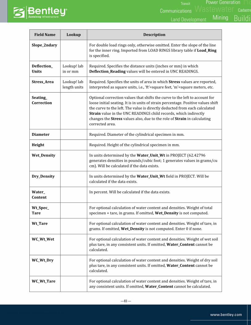
— 83 —
Field Name Lookup Description
Slope_2ndary For double load rings only, otherwise omitted. Enter the slope of the line for the inner ring. Imported from LOAD RINGS library table if Load_Ring is specified.
Deflection_ Units
Lookup! lab in or mm
Required. Specifies the distance units (inches or mm) in which Deflection_Reading values will be entered in UNC READINGS.
Stress_Area Lookup! lab length units
Required. Specifies the units of area in which Stress values are reported, interpreted as square units, i.e., ‘ft’=square feet, ‘m’=square meters, etc.
Seating_ Correction
Optional correction values that shifts the curve to the left to account for loose initial seating. It is in units of strain percentage. Positive values shift the curve to the left. The value is directly deducted from each calculated Strain value in the UNC READINGS child records, which indirectly changes the Stress values also, due to the role of Strain in calculating corrected area.
Diameter Required. Diameter of the cylindrical specimen in mm.
Height Required. Height of the cylindrical specimen in mm.
Wet_Density In units determined by the Water_Unit_Wt in PROJECT (62.42796 generates densities in pounds/cubic foot; 1 generates values in grams/cu cm). Will be calculated if the data exists.
Dry_Density In units determined by the Water_Unit_Wt field in PROJECT. Will be calculated if the data exists.
Water_ Content
In percent. Will be calculated if the data exists.
Wt_Spec_ Tare
For optional calculation of water content and densities. Weight of total specimen + tare, in grams. If omitted, Wet_Density is not computed.
Wt_Tare For optional calculation of water content and densities. Weight of tare, in grams. If omitted, Wet_Density is not computed. Enter 0 if none.
WC_Wt_Wet For optional calculation of water content and densities. Weight of wet soil plus tare, in any consistent units. If omitted, Water_Content cannot be calculated.
WC_Wt_Dry For optional calculation of water content and densities. Weight of dry soil plus tare, in any consistent units. If omitted, Water_Content cannot be calculated.
WC_Wt_Tare For optional calculation of water content and densities. Weight of tare, in any consistent units. If omitted, Water_Content cannot be calculated.

— 84 —
Field Name Lookup Description
Notes Optional field for entry of any useful information about the test. Not reported in standard gINT reports.
UNCONF COMPR table notes:
• None of the fields are captioned.
UNC READINGS table fields
Field Name Description
Load_ Reading
Observed value of load ring deflection in units particular to the measuring device. Converted to a load value through the specified load ring calibration.
Deflection_ Reading
Observed value of height deflection of the compressing platen, in units specified in Deflection_Units. In the first UNC READINGS row, this value is assumed to be the starting value of the gauge, and later UNC READINGS rows deduct the initial value from their own deflection readings when Strain is computed.
Stress Calculated. The average amount of force exerted per unit area, in the area units specified in Stress_Area.
Strain Calculated. Percentage of the original height of the specimen represented by the difference between the current and original Deflection_Reading values.
UNC READINGS table notes:
• None of the fields can be deleted or renamed (although they can be captioned) in DATA DESIGN.
• No fields have an associated lookup. • No fields are captioned.
Setting up Load Ring Calibrations in the Library Table The Load_Reading value in each readings record is an observed value of load ring deflection in units particular to the measuring device. This value must be converted to a load value in force units (such as psi) for it to be used in stress calculations. This conversion is accomplished by means of a load ring calibration curve, which defines the relationship between deflection units and load units.
• For a single ring the curve is linear with an intercept of zero. To define the calibration for a single ring, only the Slope_Initial field needs to be defined.
• For a double ring, instead of a single, linear relationship between deflection units and load units, the relationship curve has two lines with different slopes, and a

— 85 —
break point defining where one ends and the other begins, as shown:
For a double ring unit, Slope_Initial, Slope_Break and Slope_2ndary must all be defined.
• For a load cell, there is no calibration, as the load force is provided directly and doesn’t need to be converted. In this situation, you create a load ring calibration in the LOAD RINGS library table with a slope of 1, and reference this calibration in the UNCONF COMPR record.
These calibration values can be entered directly into the parent UNCONF COMPR row. Alternately, they can be defined in a named row in the LOAD RINGS library table, and referenced via the Load_Ring field in UNCONF COMPR. On a save, if a Load_Ring name as been supplied, gINT will copy the calibration parameters from the LOAD RINGS library table to the corresponding fields in the UNCONF COMPR record.
The LOAD RINGS library table contains the following fields:
Field Name Description
Ring_ID Specifies the name of a load ring calibration. When selecting a value for the Load_Ring field in the UNCONF COMPR table in INPUT, the drop-down list is populated with the names from Ring_ID in the LOAD RINGS library table.

— 86 —
Field Name Description
Slope_Initial Required. If load is electronically measured (using a load cell), enter ‘1’. For single load rings, enter the slope of the load-vs.-dial-units line. For double load rings, enter the slope of the line for the outer ring.
Slope_Break For double load rings only, otherwise omitted. Enter the load dial reading corresponding to the point where the inner ring begins to deflect.
Slope_2ndary For double load rings only, otherwise omitted. Enter the slope of the line for the inner ring.
Slope Units Optional field for documentation purposes only. Identifies the units used for load (Y axis) when calculating slopes.
Notes Optional field for documentation purposes.
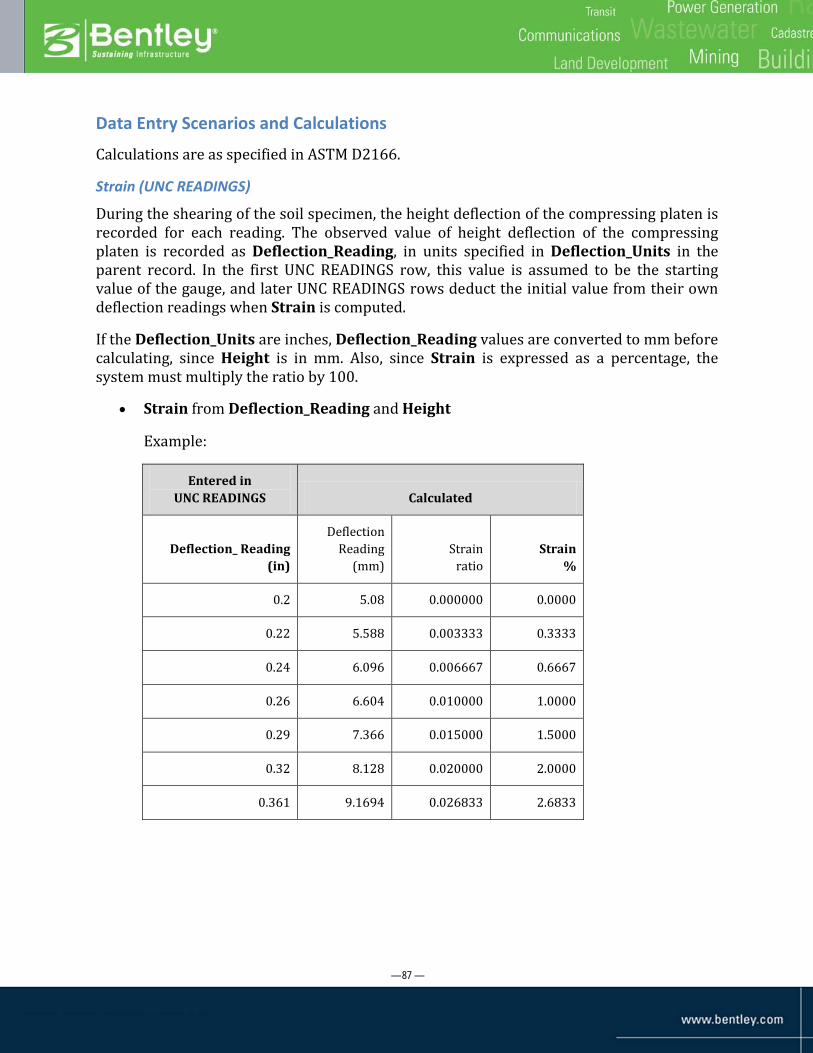
— 87 —
Data Entry Scenarios and Calculations
Calculations are as specified in ASTM D2166.
Strain (UNC READINGS)
During the shearing of the soil specimen, the height deflection of the compressing platen is recorded for each reading. The observed value of height deflection of the compressing platen is recorded as Deflection_Reading, in units specified in Deflection_Units in the parent record. In the first UNC READINGS row, this value is assumed to be the starting value of the gauge, and later UNC READINGS rows deduct the initial value from their own deflection readings when Strain is computed.
If the Deflection_Units are inches, Deflection_Reading values are converted to mm before calculating, since Height is in mm. Also, since Strain is expressed as a percentage, the system must multiply the ratio by 100.
• Strain from Deflection_Reading and Height
Example:
Entered in UNC READINGS Calculated
Deflection_ Reading (in)
Deflection Reading
(mm) Strain
ratio Strain
%
0.2 5.08 0.000000 0.0000
0.22 5.588 0.003333 0.3333
0.24 6.096 0.006667 0.6667
0.26 6.604 0.010000 1.0000
0.29 7.366 0.015000 1.5000
0.32 8.128 0.020000 2.0000
0.361 9.1694 0.026833 2.6833
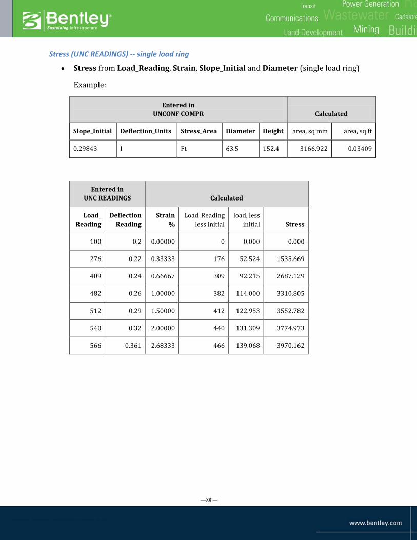
— 88 —
Stress (UNC READINGS) -- single load ring
• Stress from Load_Reading, Strain, Slope_Initial and Diameter (single load ring)
Example:
Entered in UNCONF COMPR Calculated
Slope_Initial Deflection_Units Stress_Area Diameter Height area, sq mm area, sq ft
0.29843 I Ft 63.5 152.4 3166.922 0.03409
Entered in UNC READINGS Calculated
Load_ Reading
Deflection Reading
Strain %
Load_Reading less initial
load, less initial Stress
100 0.2 0.00000 0 0.000 0.000
276 0.22 0.33333 176 52.524 1535.669
409 0.24 0.66667 309 92.215 2687.129
482 0.26 1.00000 382 114.000 3310.805
512 0.29 1.50000 412 122.953 3552.782
540 0.32 2.00000 440 131.309 3774.973
566 0.361 2.68333 466 139.068 3970.162

— 89 —
Stress (UNC READINGS) -- dual load ring
• Stress for ( Load_Reading(n) — Load_Reading(1) ) ≤ Slope_Break
As long as the stress for a reading is below the Slope_Break value, the calculations are the same as for a single load ring.
• Stress for ( Load_Reading(n) — Load_Reading(1) ) > Slope_Break
If the stress for a reading exceeds the Slope_Break, the Slope_2ndary field is brought into the stress calculation.
Example:
Entered in UNCONF COMPR
Slope_Initial
Slope_Break Slope_2ndary Deflection_Units Stress_Area Diameter Height
0.29843 382 0.75229 I Ft 63.5 152.4
Entered in UNC READINGS Calculated
Load_ Reading Strain Load_Reading less initial load
area, sq mm
area, sq ft Stress
100 0.00000 0 0 3166.92 0.03409 0.000
276 0.33333 176 52.52368 3166.92 0.03409 1535.669
409 0.66667 309 92.21487 3166.92 0.03409 2687.129
482 1.00000 382 114.00026 3166.92 0.03409 3310.805
512 1.50000 412 136.56896 3166.92 0.03409 3946.216
540 2.00000 440 157.63308 3166.92 0.03409 4531.751
566 2.68333 466 177.19262 3166.92 0.03409 5058.543
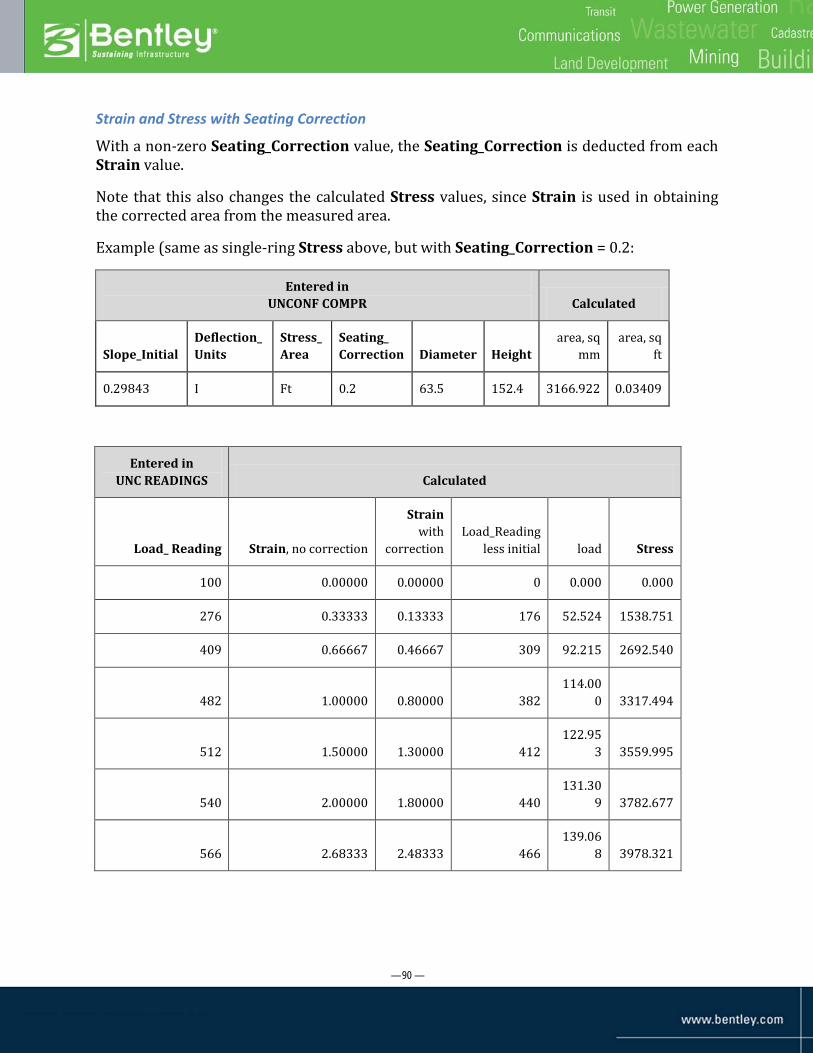
— 90 —
Strain and Stress with Seating Correction
With a non-zero Seating_Correction value, the Seating_Correction is deducted from each Strain value.
Note that this also changes the calculated Stress values, since Strain is used in obtaining the corrected area from the measured area.
Example (same as single-ring Stress above, but with Seating_Correction = 0.2:
Entered in UNCONF COMPR Calculated
Slope_Initial Deflection_ Units
Stress_ Area
Seating_ Correction Diameter Height
area, sq mm
area, sq ft
0.29843 I Ft 0.2 63.5 152.4 3166.922 0.03409
Entered in UNC READINGS Calculated
Load_ Reading Strain, no correction
Strain with
correction Load_Reading
less initial load Stress
100 0.00000 0.00000 0 0.000 0.000
276 0.33333 0.13333 176 52.524 1538.751
409 0.66667 0.46667 309 92.215 2692.540
482 1.00000 0.80000 382 114.00
0 3317.494
512 1.50000 1.30000 412 122.95
3 3559.995
540 2.00000 1.80000 440 131.30
9 3782.677
566 2.68333 2.48333 466 139.06
8 3978.321

— 91 —
Some Typical Reports
UNCONFINED (Unconfined Compression Test)
This graph report combines the data from all specimens in the project onto one report page for each five UNC COMPR rows. This makes it possible to visually compare stress-strain curves for various point-depth combinations. A sample appears below:

— 92 —
The graph in the upper portion displays multiple stress-strain curves (up to 5 per report page). The lower portion provides selected data for each of the stress-strain curves, including classifications derived from the Atterberg data and fines content for the same specimen.
Notice that each curve is for one specimen, that is, one point-depth combination. Each page in the report contains a maximum of five curves, each identified under ‘Specimen Identification’ (including legend symbols) at the bottom. The specimens presented as curves and table data on each page are not necessarily grouped together functionally; after each page fills up with five specimens, a new page is started.

— 93 —
Consolidation
Background
Consolidation is a process by which soils decrease in volume. It occurs when stress is applied to a soil that causes the soil particles to pack together more tightly, therefore reducing its bulk volume. When this occurs in a soil that is saturated with water, water will be squeezed out of the soil. The magnitude of consolidation can be predicted by many different methods. In the Classical Method, developed by Karl von Terzaghi, soils are tested with an oedometer test to determine their compression index. This can be used to predict the amount of consolidation.
When stress is removed from a consolidated soil, the soil will rebound, regaining some of the volume it had lost in the consolidation process. If the stress is reapplied, the soil will consolidate again along a recompression curve, defined by the recompression index. The soil which had its load removed is considered to be overconsolidated. This is the case for soils which have previously had glaciers on them. The highest stress that it has been subjected to is termed the preconsolidation stress. The over consolidation ratio or OCR is defined as the highest stress experienced divided by the current stress. A soil which is currently experiencing its highest stress is said to be normally consolidated and to have an OCR of one. A soil could be considered underconsolidated immediately after a new load is applied but before the excess pore water pressure has had time to dissipate.
Testing consists of trimming a cylinder of soil from a sampler into a confining ring, and placing a pair of porous plates that just fit inside the ring on the top and bottom ends of the cylinder. This soil “sandwich” is placed inside an open-top water container, enabling the water to enter and leave the soil through the porous plates. All of this is placed inside a vertical compression device (oedometer) that can control the applied load and measure specimen height deflection.
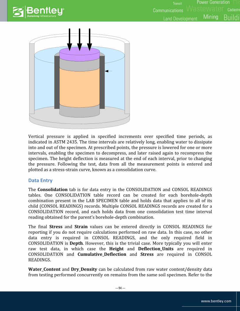
— 94 —
Vertical pressure is applied in specified increments over specified time periods, as indicated in ASTM 2435. The time intervals are relatively long, enabling water to dissipate into and out of the specimen. At prescribed points, the pressure is lowered for one or more intervals, enabling the specimen to decompress, and later raised again to recompress the specimen. The height deflection is measured at the end of each interval, prior to changing the pressure. Following the test, data from all the measurement points is entered and plotted as a stress-strain curve, known as a consolidation curve.
Data Entry
The Consolidation tab is for data entry in the CONSOLIDATION and CONSOL READINGS tables. One CONSOLIDATION table record can be created for each borehole-depth combination present in the LAB SPECIMEN table and holds data that applies to all of its child (CONSOL READINGS) records. Multiple CONSOL READINGS records are created for a CONSOLIDATION record, and each holds data from one consolidation test time interval reading obtained for the parent’s borehole-depth combination.
The final Stress and Strain values can be entered directly in CONSOL READINGS for reporting if you do not require calculations performed on raw data. In this case, no other data entry is required in CONSOL READINGS, and the only required field in CONSOLIDATION is Depth. However, this is the trivial case. More typically you will enter raw test data, in which case the Height and Deflection_Units are required in CONSOLIDATION and Cumulative_Deflection and Stress are required in CONSOL READINGS.
Water_Content and Dry_Density can be calculated from raw water content/density data from testing performed concurrently on remains from the same soil specimen. Refer to the

— 95 —
“WC Density” chapter for the specifics of calculations and calculation scenarios, which are the same in that tab for corresponding fields as here. Water content and wet/dry density data are not required in a parent CONSOLIDATION record for calculations, but they are required if you want to include this specimen in the CONSOL VOID RATIO report.
The rest of the fields in both tables are for documentation and potential reporting, but not included in current standard reports

— 96 —
CONSOLIDATION table fields
Field Name Caption Lookup Description
PointID In combination with Depth, specifies the parent LAB SPECIMEN record. (Specified in the object selector).
Depth In combination with PointID, specifies the parent LAB SPECIMEN record.
Deflection_ Units
Lookup!lab in or mm
Required for strain calculations. Specifies the distance units (inches or mm) in which Cumulative_Deflection values will be entered in CONSOL READINGS.
Diameter Required if performing strain calculations. Diameter of the cylindrical specimen in mm.
Height Required if performing strain calculations. Height of the cylindrical specimen in mm.
Wet_Density In units determined by the Water_Unit_Wt in PROJECT (62.42796 generates densities in pounds/cubic foot; 1 generates values in grams/cu cm). Will be calculated if the data exists.
Dry_Density In units determined by the Water_Unit_Wt field in PROJECT. Will be calculated if the data exists. Required for void ratio reporting (CONSOL VOID RATIO report).
Water_ Content
In percent. Will be calculated if the data exists.
Wt_Spec_ Tare
Wt Specimen + Tare
For optional calculation of water content and densities. Weight of total specimen + tare, in grams. If omitted, Wet_Density is not computed.
Wt_Tare For optional calculation of water content and densities. Weight of tare, in grams. If omitted, Wet_Density is not computed. Enter 0 if none.
WC_Wt_Wet Water Content Wet Wt+Tare
For optional calculation of water content and densities. Weight of wet soil plus tare, in any consistent units. If omitted, Water_Content cannot be calculated.
WC_Wt_Dry Water Content Dry Wt+Tare
For optional calculation of water content and densities. Weight of dry soil plus tare, in any consistent units. If omitted, Water_Content cannot be calculated.

— 97 —
Field Name Caption Lookup Description
WC_Wt_Tare Water Content Wt Tare
For optional calculation of water content and densities. Weight of tare, in any consistent units. If omitted, Water_Content cannot be calculated.
Dry_Density_ After
After-test dry density value. Optional, not calculated.
Water_ Content_ After
After-test water content value, in percent. Optional, not calculated.
P0 In-situ overburden pressure. Not calculated. Optional entry.
Pmax Maximum Past Pressure. Not calculated. Optional entry.
Cr Slope of rebound portion of curve. Not calculated. Optional entry.
Cc Slope of virgin compression portion of curve. Not calculated. Optional entry.
Cv50_Typical Type coefficient of consolidation at 50% consolidation. Optional entry. Not calculated from the readings.
Cv90_Typical Type coefficient of consolidation at 90% consolidation. Optional entry. Not calculated from the readings.
Note_1 Optional entry.
Note_2 Optional entry.
CONSOLIDATION table notes:
• P0, Pmax, Cr, Cc, Cv50_Typical, Cv90_Typical, Note_1 and Note_2 can all be deleted or modified. The other fields cannot.
CONSOL READINGS table fields
Field Name Description
Stress Vertical stress applied to the specimen for the interval at the end of which this reading was taken. The Stress readings can be in any units that are consistent with the X axis scale on consolidation reports. These values are required and reported, but not used in calculations.
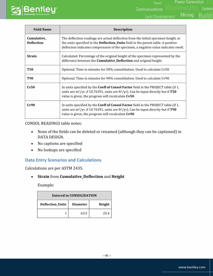
— 98 —
Field Name Description
Cumulative_ Deflection
The deflection readings are actual deflection from the initial specimen height, in the units specified in the Deflection_Units field in the parent table. A positive deflection indicates compression of the specimen, a negative value indicates swell.
Strain Calculated. Percentage of the original height of the specimen represented by the difference between the Cumulative_Deflection and original height.
T50 Optional. Time in minutes for 50% consolidation. Used to calculate Cv50.
T90 Optional. Time in minutes for 90% consolidation. Used to calculate Cv90.
Cv50 In units specified by the Coeff of Consol Factor field in the PROJECT table (if 1, units are m2/yr, if 10.76391, units are ft2/yr). Can be input directly but if T50 value is given, the program will recalculate Cv50.
Cv90 In units specified by the Coeff of Consol Factor field in the PROJECT table (if 1, units are m2/yr, if 10.76391, units are ft2/yr). Can be input directly but if T90 value is given, the program will recalculate Cv90.
CONSOL READINGS table notes:
• None of the fields can be deleted or renamed (although they can be captioned) in DATA DESIGN.
• No captions are specified • No lookups are specified
Data Entry Scenarios and Calculations
Calculations are per ASTM 2435.
• Strain from Cumulative_Deflection and Height
Example:
Entered in CONSOLIDATION
Deflection_Units Diameter Height
I 63.5 25.4

— 99 —
Entered in CONSOL READINGS Calculated
Stress Cumulative_
Deflection Deflection Readg mm
Strain Ratio Strain %
150 0.0017 0.04318 0.0017 0.17
300 0.0029 0.07366 0.0029 0.29
550 0.005 0.127 0.005 0.5
1100 0.012 0.3048 0.012 1.2
2200 0.0291 0.73914 0.0291 2.91
300 0.0121 0.30734 0.0121 1.21
2200 0.0309 0.78486 0.0309 3.09
4400 0.0663 1.68402 0.0663 6.63
8800 0.1427 3.62458 0.1427 14.27
2200 0.1245 3.1623 0.1245 12.45
300 0.0938 2.38252 0.0938 9.38
150 0.073 1.8542 0.073 7.3

— 100 —
Some Typical Reports
CONSOL STRAIN (Consolidation Test) graph
This graph report combines the data from all specimens in the project onto one report page for each five CONSOLIDATION rows. This makes it possible to visually compare consolidation curves for various point-depth combinations. A sample appears below:

— 101 —
The graph in the upper portion displays multiple stress-strain curves (up to 5 per report page). The lower portion provides selected data for each of the stress-strain curves, including classifications derived from the Atterberg data and fines content for the same specimen.
Notice that each curve is for one specimen, that is, one point-depth combination. Each page in the report contains a maximum of five curves, each identified under ‘Specimen Identification’ (including legend symbols) at the bottom. The specimens presented as curves and table data on each page are not necessarily grouped together functionally; after each page fills up with five specimens, a new page is started.

— 102 —
CONSOL VOID RATIO graph
This graph report is equivalent to the CONSOLIDATION graph, but plots void ratio on the Y axis rather than strain.

— 103 —
Direct Shear
Background
A direct shear test is a laboratory test used by geotechnical engineers to find the shear strength parameters of soil. In the U.S., the standard defining how the test should be performed is ASTM D 3080.
The test is performed on three or four specimens from a relatively undisturbed soil sample. A specimen is placed in a shear box which has two stacked rings to hold the sample; the contact between the two rings is at approximately the mid-height of the sample. A confining stress is applied vertically to the specimen, and the upper ring is pulled laterally until the sample fails, or through a specified strain. The load applied and the strain induced is recorded at frequent intervals to determine a stress-strain curve for the confining stress.
Direct shear tests can be performed under several conditions. The sample is normally saturated before the test is run, but can be run at the in-situ moisture content. The rate of strain can be varied to create a test of undrained or drained conditions, depending whether the strain is applied slowly enough for water in the sample to prevent pore-water pressure buildup.
Several specimens are tested at varying confining stresses to determine the shear strength parameters, the soil cohesion (c) and the angle of internal friction (commonly friction angle) (φ). The results of the tests on each specimen are plotted on a graph with the peak (or residual) stress on the x-axis and the confining stress on the y-axis. The y-intercept of the curve which fits the test results is the cohesion, and the slope of the line or curve is the friction angle.
Data Entry
The Direct Shear tab is for data entry in the DIRECT SHEAR and DSHR READINGS tables. The Ring_Area and Ring_Height are directly entered in the upper grid, and are used in calculations. The other DIRECT SHEAR fields (other than Depth) are either calculated or optional.
The fields in the lower (DSHR READINGS) grid are for entry of Normal_Stress and Failure_Stress values observed for each reading. A point is plotted in standard reports from each Normal_Stress, Failure_Stress pair (X and Y respectively). Cohesion_Calc and Friction_Angle_Calc in the upper grid are calculated as the intercept and slope (respectively) of the best-fit line between these readings points. Readings where the Not_Used_In_Calculations field in the child record is checked are not included in the slope/intercept calculations.
Water content and density data can optionally be entered in the child records, with their values averaged to generate values in the corresponding fields in the parent. This is for

— 104 —
reporting purposes. Water content and density calculations are equivalent to those performed elsewhere in Lab Testing. The result values can be entered directly in the upper grid if averaging the moisture and density data by reading is not needed.
If the Cohesion_Calc calculates to less than zero (0), the Friction_Angle_Calc will be recalculated so that the best fit line is forced through the origin and the Cohesion_Calc is set to zero (0).
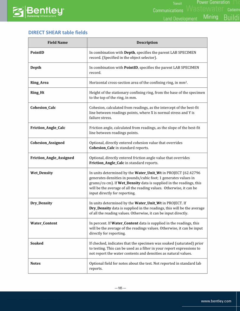
— 105 —
DIRECT SHEAR table fields
Field Name Description
PointID In combination with Depth, specifies the parent LAB SPECIMEN record. (Specified in the object selector).
Depth In combination with PointID, specifies the parent LAB SPECIMEN record.
Ring_Area Horizontal cross-section area of the confining ring, in mm2.
Ring_Ht Height of the stationary confining ring, from the base of the specimen to the top of the ring, in mm.
Cohesion_Calc Cohesion, calculated from readings, as the intercept of the best-fit line between readings points, where X is normal stress and Y is failure stress.
Friction_Angle_Calc Friction angle, calculated from readings, as the slope of the best-fit line between readings points.
Cohesion_Assigned Optional, directly entered cohesion value that overrides Cohesion_Calc in standard reports.
Friction_Angle_Assigned Optional, directly entered friction angle value that overrides Friction_Angle_Calc in standard reports.
Wet_Density In units determined by the Water_Unit_Wt in PROJECT (62.42796 generates densities in pounds/cubic foot; 1 generates values in grams/cu cm). If Wet_Density data is supplied in the readings, this will be the average of all the reading values. Otherwise, it can be input directly for reporting.
Dry_Density In units determined by the Water_Unit_Wt in PROJECT. If Dry_Density data is supplied in the readings, this will be the average of all the reading values. Otherwise, it can be input directly.
Water_Content In percent. If Water_Content data is supplied in the readings, this will be the average of the readings values. Otherwise, it can be input directly for reporting.
Soaked If checked, indicates that the specimen was soaked (saturated) prior to testing. This can be used as a filter in your report expressions to not report the water contents and densities as natural values.
Notes Optional field for notes about the test. Not reported in standard lab reports.

— 106 —
DIRECT SHEAR table notes:
• None of the fields can be deleted or renamed (although they can be captioned) in DATA DESIGN except Notes.
• No captions are specified • No lookups are specified

— 107 —
DSHR READINGS table fields
Field Name Caption Description
Reading Normal Stress Normal pressure reading, in psf. Plotted in the DIRECT SHEAR report along the X axis, one point plotted for each reading. Used in calculating Calculated_Cohesion and Calculated_Friction_Angle in the parent record.
Failure_Stress The average amount of force exerted per unit area at failure, in psf. Plotted in the DIRECT SHEAR report along the Y axis, one point plotted for each reading. Used in calculating Calculated_Cohesion and Calculated_Friction_Angle in the parent record.
Wet_Density Also known as wet unit weight or total unit weight. In units determined by the Water_Unit_Wt in PROJECT (62.42796 generates densities in pounds/cubic foot; 1 generates values in grams/cu cm). Will be calculated if the data exists, or can be input directly.
Dry_Density Also known as dry unit weight. In units determined by the Water_Unit_Wt field in PROJECT. Will be calculated if the data exists, or can be input directly.
Water_Content Also known as moisture content. This value is in percent. It will be calculated if the data exists, or can be input directly.
Wt_Spec_Tare Wt Specimen + Tare
In grams. Weight of total specimen + tare. If omitted, Wet_Density is not computed.
Wt_Tare In grams. Weight of tare. If omitted, Wet_Density is not computed. Enter 0 if none.
WC_Wt_Wet Water Content Wet Wt+Tare
Weight of wet soil plus tare, in any consistent units. If omitted, Water_Content cannot be calculated.
WC_Wt_Dry Water Content Dry Wt+Tare
Weight of dry soil plus tare, in any consistent units. If omitted, Water_Content cannot be calculated.
WC_Wt_Tare Water Content Wt Tare
Weight of tare, in any consistent units. If omitted, Water_Content cannot be calculated.
Not_Used_In_Calc If checked, this readings record is omitted from the calculation of Calculated_Cohesion and Calculated_Friction_Angle in the parent record.
— 108 —
DSHR READINGS table notes:
• None of the fields can be deleted or renamed (although they can be captioned) in DATA DESIGN.
• No lookups are specified
Data Entry Scenarios and Calculations
Calculated Cohesion and Calculated Friction Angle are calculated as the intercept and slope (respectively) of the best fit line between the (Normal Stress, Failure Stress) coordinate pairs in the readings records. Calculation of this line and its resulting intercept and slope are beyond the scope of this manual.
Reporting
DIRECT SHEAR (Direct Shear Test)
This graph report combines the data from all specimens in the project onto one report page for each six DIRECT SHEAR table rows. This makes it possible to visually compare normal-failure stress lines for various point-depth combinations. A sample appears below:
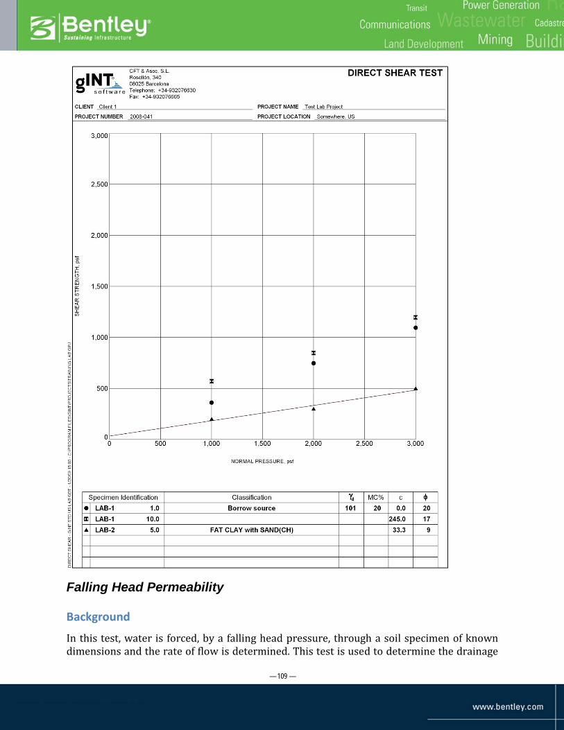
— 109 —
Falling Head Permeability
Background
In this test, water is forced, by a falling head pressure, through a soil specimen of known dimensions and the rate of flow is determined. This test is used to determine the drainage

— 110 —
characteristics of relatively fine-grained soils and is usually performed on undisturbed samples.
The objective of the falling head permeability test is to allow the water level in a small-diameter standpipe tube (burette) in a laboratory falling-head permeameter to fall from an initial position to a final position due to seepage through the soil sample. The amount of time it takes the water “head” to fall this distance is recorded. Based on Darcy’s law, a coefficient of permeability (hydraulic conductivity) is calculated. The permeameter apparatus is shown here:
(Reproduced from Day, p 373. Original is Dept. of the Army, 1970)
Some specifications for this test appear in ASTM D5084, although the gINT implementation is different in some regards. The calculations as performed in gINT are described in “Data Entry Scenarios and Calculations” on page 116.
Data Entry
Falling head permeability data is not reported in standard reports. Rather, the data is entered in order to generate a single permeability (K_Calculated, captioned as Permeability Calculated) value in the parent (FALL HEAD K) record. You can optionally enter a K_Assigned value for comparison, and/or directly enter the K_Calculated, if you just need to record an externally calculated value.
Water content/density values can optionally be computed for before-test and after-test, if you provide the source data for these fields. Moisture/density values are computed the same as elsewhere in gINT.

— 111 —
FALL HEAD K table fields
Field Name Caption Lookup Description
PointID In combination with Depth, specifies the parent LAB SPECIMEN record. (Specified in the object selector).
Depth In combination with PointID, specifies the parent LAB SPECIMEN record.
K_Assigned Permeability Assigned
Permeability value assigned by you, in case you have this from another source for comparison with the calculated value, or don’t want to calculate.
K_Calculated Permeability Calculated
Average permeability calculated from the Permeability values in the readings records. The calculation requires values in the K_Units_Fac, Initial_Head, Temperature_Units, Burette_Area, Diameter, and Height fields in the parent, and Time, Head and Temperature values for each child readings record.
K_Units_Fac Permeability Units Factor
If the calculated permeability is to be in mm/sec, no conversion is required and a value of ‘1’ is entered in K_Units_Fac. If minutes are desired rather than seconds, the factor should be multiplied by 1/60, that is, 0.0167. If cm are desired rather than mm, the factor should be divided by 10, and so on. So for units of cm/sec, the units factor would be 0.00167. Required for calculation of permeability.
Initial_Head Specifies the initial height of the water level (head) in the permeameter burette prior to the start of seepage. Any units are permitted, but must be consistent with the Head values in the readings records. Required for calculation of permeability.
Temperature_Units Lookup!lab temp units
Specifies the units entered in the Temperature field in readings records, F or C. Required for calculation of permeability.
Burette_Area Cross-sectional area of the permeameter burette tube, in mm2. Required for calculation of permeability.
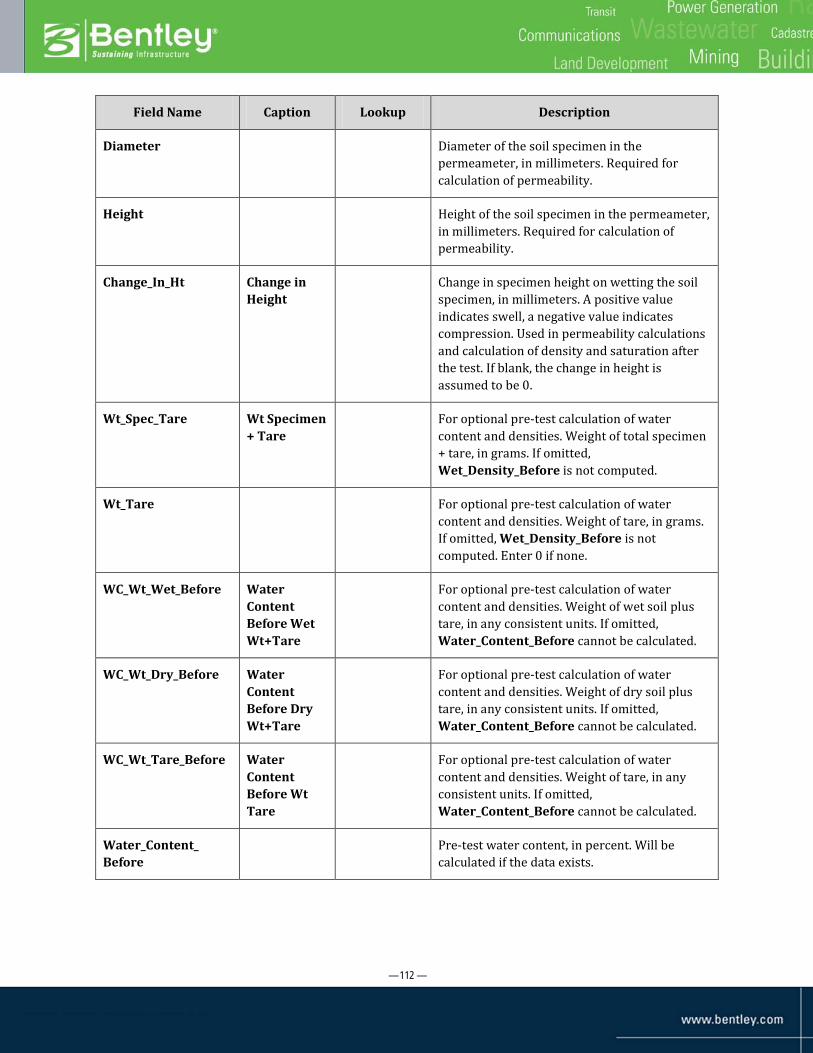
— 112 —
Field Name Caption Lookup Description
Diameter Diameter of the soil specimen in the permeameter, in millimeters. Required for calculation of permeability.
Height Height of the soil specimen in the permeameter, in millimeters. Required for calculation of permeability.
Change_In_Ht Change in Height
Change in specimen height on wetting the soil specimen, in millimeters. A positive value indicates swell, a negative value indicates compression. Used in permeability calculations and calculation of density and saturation after the test. If blank, the change in height is assumed to be 0.
Wt_Spec_Tare Wt Specimen + Tare
For optional pre-test calculation of water content and densities. Weight of total specimen + tare, in grams. If omitted, Wet_Density_Before is not computed.
Wt_Tare For optional pre-test calculation of water content and densities. Weight of tare, in grams. If omitted, Wet_Density_Before is not computed. Enter 0 if none.
WC_Wt_Wet_Before Water Content Before Wet Wt+Tare
For optional pre-test calculation of water content and densities. Weight of wet soil plus tare, in any consistent units. If omitted, Water_Content_Before cannot be calculated.
WC_Wt_Dry_Before Water Content Before Dry Wt+Tare
For optional pre-test calculation of water content and densities. Weight of dry soil plus tare, in any consistent units. If omitted, Water_Content_Before cannot be calculated.
WC_Wt_Tare_Before Water Content Before Wt Tare
For optional pre-test calculation of water content and densities. Weight of tare, in any consistent units. If omitted, Water_Content_Before cannot be calculated.
Water_Content_ Before
Pre-test water content, in percent. Will be calculated if the data exists.

— 113 —
Field Name Caption Lookup Description
Wet_Density_Before Pre-test wet density. In units determined by the Water_Unit_Wt in PROJECT (62.42796 generates densities in pounds/cubic foot; 1 generates values in grams/cu cm). Will be calculated if the data exists.
Dry_Density_Before Pre-test dry density. In units determined by the Water_Unit_Wt field in PROJECT. Will be calculated if the data exists.
WC_Wt_Wet_After Water Content After Wet Wt+Tare
For optional calculation of post-test water content and densities. Weight of wet soil plus tare, in any consistent units. If omitted, Water_Content_After cannot be calculated.
WC_Wt_Dry_After Water Content After Dry Wt+Tare
For optional calculation of post-test water content and densities. Weight of dry soil plus tare, in any consistent units. If omitted, Water_Content_After cannot be calculated.
WC_Wt_Tare_After Water Content After Wt Tare
For optional calculation of post-test water content and densities. Weight of tare, in any consistent units. If omitted, Water_Content_After cannot be calculated.
Water_Content_After After-test water content value, in percent.
Wet_Density_After Post-test wet density in units determined by the Water_Unit_Wt in PROJECT (62.42796 generates densities in pounds/cubic foot; 1 generates values in grams/cu cm). Will be calculated if the data exists.
Dry_Density_After Post-test dry density in units determined by the Water_Unit_Wt in PROJECT.
Time_Units Not used by calculations. For documentation of the time units used in the readings table.
Chamber_Pressure For documentation purposes. Not used in calculations.
Back_Pressure For documentation purposes. Not used in calculations.
Fluid_Used For documentation purposes. Not used in calculations.

— 114 —
Field Name Caption Lookup Description
Note_1 For documentation purposes.
Note_2 For documentation purposes.
Note_3 For documentation purposes.
FALL HEAD K table notes:
• No fields can be deleted or renamed (although they can be captioned) in DATA DESIGN except the following: Time_Units, Chamber_Pressure, Back_Pressure, Fluid_Used, Note_1, Note_2, and Note_3.
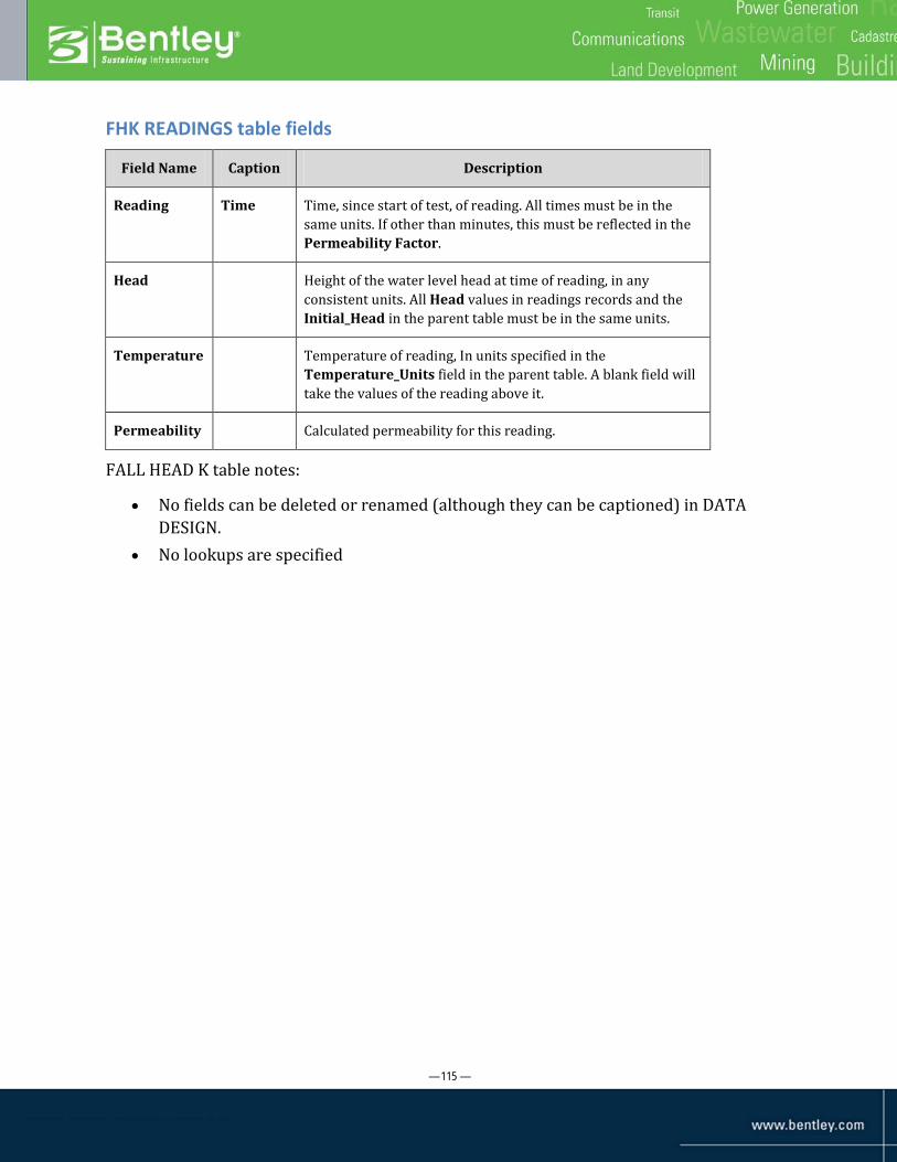
— 115 —
FHK READINGS table fields
Field Name Caption Description
Reading Time Time, since start of test, of reading. All times must be in the same units. If other than minutes, this must be reflected in the Permeability Factor.
Head Height of the water level head at time of reading, in any consistent units. All Head values in readings records and the Initial_Head in the parent table must be in the same units.
Temperature Temperature of reading, In units specified in the Temperature_Units field in the parent table. A blank field will take the values of the reading above it.
Permeability Calculated permeability for this reading.
FALL HEAD K table notes:
• No fields can be deleted or renamed (although they can be captioned) in DATA DESIGN.
• No lookups are specified

— 116 —
Data Entry Scenarios and Calculations
Water Content Calculations
Refer to “Water Content / Density” on page 17—the calculations are the same.
Permeability, with Constant Temperature less than or equal 20° C
Permeabilityavg = Σ(1 to n)Permeabilityn
n
where:
Permeabilityn = Burette_Area x (Height + Chg_in_Ht)
x Ln( Headinit
) x temp_correction sample_area x Timen Headn
sample area = π x (Diameter/2)2
temp _correction =
10
( 1301 ) — 1.30233 998.333 + (8.1855 x (Tempn-20))+ (0.00585 x (Tempn-20)2)
(Tempn values are in °C)
Example:
Entered in FALL HEAD K Calculated
K_Units_ Factor
Initial_ Head
Burette_ Area mm2
Diameter mm
sample area mm2
K_ Calculated
1 52.4 125 61.72
2991.863 3.22E-04
Entered in FHK READINGS Calculated
Time (min)
Head (mm) Temp
temp correction permeability
corrected permeability
K x units factor
35 51.8 18 1.053263291 3.53E-04 3.72E-04 3.72E-04
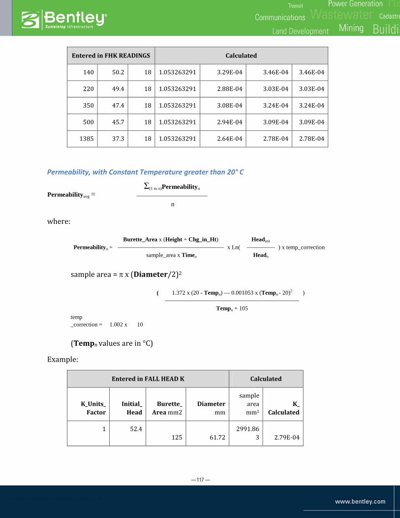
— 117 —
Entered in FHK READINGS Calculated
140 50.2 18 1.053263291 3.29E-04 3.46E-04 3.46E-04
220 49.4 18 1.053263291 2.88E-04 3.03E-04 3.03E-04
350 47.4 18 1.053263291 3.08E-04 3.24E-04 3.24E-04
500 45.7 18 1.053263291 2.94E-04 3.09E-04 3.09E-04
1385 37.3 18 1.053263291 2.64E-04 2.78E-04 2.78E-04
Permeability, with Constant Temperature greater than 20° C
Permeabilityavg = Σ(1 to n)Permeabilityn
n
where:
Permeabilityn = Burette_Area x (Height + Chg_in_Ht)
x Ln( Headinit
) x temp_correction sample_area x Timen Headn
sample area = π x (Diameter/2)2
temp _correction = 1.002 x 10
( 1.372 x (20 - Tempn) — 0.001053 x (Tempn - 20)2 )
Tempn + 105
(Tempn values are in °C)
Example:
Entered in FALL HEAD K Calculated
K_Units_ Factor
Initial_ Head
Burette_ Area mm2
Diameter mm
sample area mm2
K_ Calculated
1 52.4 125 61.72
2991.863 2.79E-04
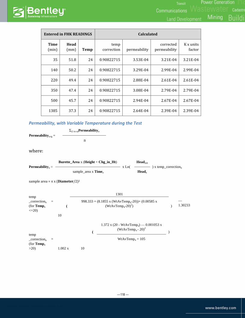
— 118 —
Entered in FHK READINGS Calculated
Time (min)
Head (mm) Temp
temp correction permeability
corrected permeability
K x units factor
35 51.8 24 0.90822715 3.53E-04 3.21E-04 3.21E-04
140 50.2 24 0.90822715 3.29E-04 2.99E-04 2.99E-04
220 49.4 24 0.90822715 2.88E-04 2.61E-04 2.61E-04
350 47.4 24 0.90822715 3.08E-04 2.79E-04 2.79E-04
500 45.7 24 0.90822715 2.94E-04 2.67E-04 2.67E-04
1385 37.3 24 0.90822715 2.64E-04 2.39E-04 2.39E-04
Permeability, with Variable Temperature during the Test
Permeabilityavg = Σ(1 to n)Permeabilityn
n
where:
Permeabilityn = Burette_Area x (Height + Chg_in_Ht)
x Ln( Headinit
) x temp_correctionn sample_area x Timen Headn
sample area = π x (Diameter/2)2
temp _correctionn (for Tempn <=20)
10
(
1301
) — 1.30233
= 998.333 + (8.1855 x (WtAvTempn-20))+ (0.00585 x (WtAvTempn-20)2)
temp _correctionn (for Tempn >20)
1.002 x 10
(
1.372 x (20 - WtAvTempn) — 0.001053 x (WtAvTempn - 20)2
)
= WtAvTempn + 105
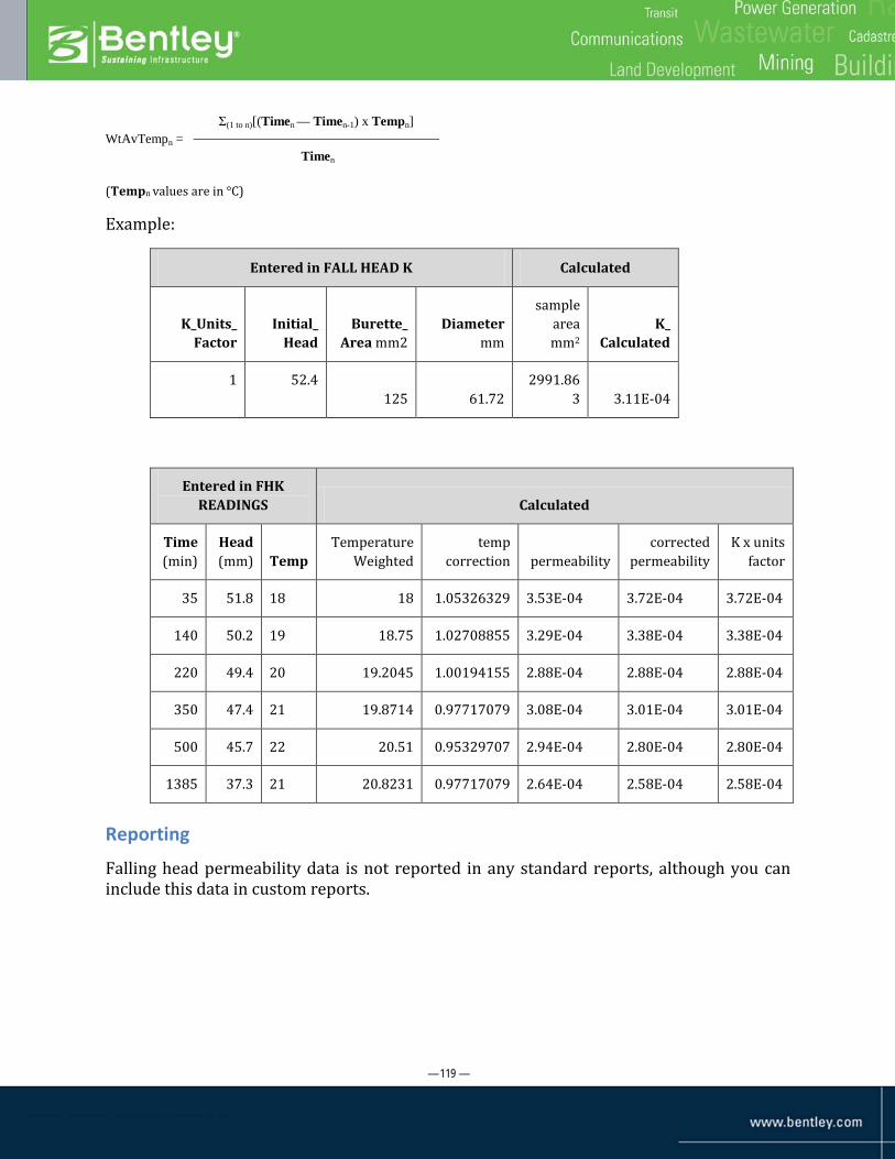
— 119 —
WtAvTempn = Σ(1 to n)[(Timen — Timen-1) x Tempn]
Timen
(Tempn values are in °C)
Example:
Entered in FALL HEAD K Calculated
K_Units_ Factor
Initial_ Head
Burette_ Area mm2
Diameter mm
sample area mm2
K_ Calculated
1 52.4 125 61.72
2991.863 3.11E-04
Entered in FHK READINGS Calculated
Time (min)
Head (mm) Temp
Temperature Weighted
temp correction permeability
corrected permeability
K x units factor
35 51.8 18 18 1.05326329 3.53E-04 3.72E-04 3.72E-04
140 50.2 19 18.75 1.02708855 3.29E-04 3.38E-04 3.38E-04
220 49.4 20 19.2045 1.00194155 2.88E-04 2.88E-04 2.88E-04
350 47.4 21 19.8714 0.97717079 3.08E-04 3.01E-04 3.01E-04
500 45.7 22 20.51 0.95329707 2.94E-04 2.80E-04 2.80E-04
1385 37.3 21 20.8231 0.97717079 2.64E-04 2.58E-04 2.58E-04
Reporting
Falling head permeability data is not reported in any standard reports, although you can include this data in custom reports.

— 120 —
Appendix A -- Suggested Field Defaults
Table Field Description
PROJECT Water_Unit_Wt 62.42796 = pounds/cubic foot, 1 = metric tons/cubic meter,9.806 = kN/cubic meter
Coeff_of_Consol_Factor 10.76391 = square ft/year, 1 = square meters/year.
WC DENSITY Diameter Soil sample cylinder diameter in mm
Height Soil sample cylinder height in mm
SIEVE Weighing_Method C(umulative) or I(ncremental)
HYDROMETER Temperature_Units_Test C(entigrade) or F(arhenheit)
HydrometerID Most commonly used hydrometer. Taken from the HYDROMETER CALIBRATIONS library table
FINE SG Readings_Temperature_Units C(entigrade) or F(ahrenheit)
COMPACTION Method Identification of most commonly used compaction test method. Can be taken from the COMPACTION METHODS library data table.
Volume_Units Cubic Ft (feet), M(eters), I(nches), cm (centimeters), or mm (millimeters)
Weight_Units P(ounds), KG (kilograms), G(rams), N(ewtons), KN (kilonewtons)
UNCONF COMPR Load_Ring Identification of most commonly used load ring. Taken from the LOAD RINGS library data table in Data Design
Deflection_Units I(nches) or M(illimeters)
Stress_Area Square Ft (feet), M(eters), I(nches), cm (centimeters), or mm (millimeters)
Diameter Specimen diameter in mm
Height Specimen height in mm
CONSOLIDATION Deflection_Units I(nches) or M(illimeters)
Diameter Specimen diameter in mm

— 121 —
Table Field Description
Height Specimen height in mm
DIRECT SHEAR Ring_Area mm
Ring_Ht mm
FALL HEAD K K_Units_Fac 1 indicates units of mm/time unit used in the readings. E.g., if time units are minutes and want final results to be cm/sec, the units factor would be 0.00167.
Temperature_Units C(entigrade) or F(ahrenheit)
Burette_Area square mm
Diameter Specimen diameter in mm
Height Specimen height in mm

— 122 —
Appendix B -- Lab Database Structure Manipulation
There are various ways you can alter or add to the database structure of a database that has lab testing support. Normally you can make any of these changes without disrupting calculations or reports. However, if you have created any custom SQL statements, these will need to be changed to match the new database structure.
Adding Tables to Lab Testing Support
You can add additional tables to lab testing support. There are two possible scenarios:
• Parent is LAB SPECIMEN, relationship is one-to-one • Parent is LAB SPECIMEN, relationship is one-to-many
Parent is LAB SPECIMEN, relationship is one-to-one
A new table for test records will typically have a one-to-one relationship with the standard parent table, LAB SPECIMEN. In this scenario, it will be possible to add as many as (but no more than) one record in the new table for each borehole-depth combination in the project database.
To add a new lab testing table with a one-to-one relationship to the parent LAB SPECIMEN, do the following:
1. Go to DATA DESIGN Project Database and open the database or data template.
2. Choose Tables New and specify the following property settings:

— 123 —
Property Value Comments
Name (any valid table name for the new table)
Key Set PointID, Depth
Parent Table LAB SPECIMEN
One to One Relation
checked
Group Name Lab Testing Selecting this tab is not required, but typically you want all lab tables included in the Lab Testing tab.
Parent is LAB SPECIMEN, relationship is one-to-many
You may have certain tests that are performed at multiple depths within the same specimen. In this case you need to be able to specify the depth of the lab specimen separately from the depth of each test, but associate all of the tests to a single lab specimen (borehole-depth combination) for reporting. You would create the test’s table as a child of LAB SPECIMEN with a one-to-many relationship, as follows:
1. Go to DATA DESIGN Project Database and open the database.
2. Choose Tables New and specify the following property settings:
Property Value
Name (any valid table name for the new table)
Key Set PointID, Depth
Parent Table LAB SPECIMEN
One to One Relation
unchecked
Group Name Lab Testing
3. The table is created. Notice that three fields are created automatically: PointID, LABSPECIMEN_Depth, and Depth. In INPUT all three fields are required: the PointID and LABSPECIMEN_Depth are selected from object selectors, and the Depth field is a column in the table grid.

— 124 —
Making LAB SPECIMEN a Child of a Non-POINT Table
By default, when you create lab testing, the LAB SPECIMEN table is created as one-to-many child of POINT, and the other lab testing tables are created as children (or grandchildren) of LAB SPECIMEN. This is as described in the section called “Relational Database Structure” on page 13. However, LAB SPECIMEN can be moved in the structure so that it is a child of some table other than POINT. For example, LAB SPECIMEN can be a child of SAMPLE.
The parent of the LAB SPECIMEN table cannot be changed once it has data. Therefore, the easiest approach is to change the parent immediately after adding lab testing support but before entering any lab testing data. You would do this as follows:
1. Add lab testing support to your database (as described in “Adding Lab Testing Support” on page 6)
2. Go to DATA DESIGN Project Database.
3. Select LAB SPECIMEN in the object selector.
4. Click the Properties icon.
5. In the Parent Table property, select the new parent (such as SAMPLE).
6. Go to INPUT Lab Specimen. Click in the Depth field. Notice that the available set of depths for a lab specimen in a given borehole are the set of depths in that borehole’s SAMPLE table (or whichever parent table you specified).
If you already have lab testing data in your database and want to change the parent of LAB SPECIMEN, the process is more complicated. You would do the following:
1. Write a correspondence file using SQL statements that port the data from LAB SPECIMEN and its children in the source database to the target. Refer to Help Index Correspondence Files and Help Index Sql for more information, or consult with gINT Technical Support.

— 125 —
2. In INPUT, clone the existing database to a new, empty database (File New Project Clone Project).
3. In DATA DESIGN, reassign the parent of LAB SPECIMEN in the new database.
4. In INPUT, select File Import/Export Import from Database and specify the correspondence file you created.
Extending the Keysets of Lab Testing Tables
When you add lab testing support, the default structure is for LAB SPECIMEN to have a one-to-many relationship with its parent POINT, and for each of the non-readings (ATTERBERG, SIEVE, HYDROMETER, etc.) tables to have a one-to-one relationship with its parent LAB SPECIMEN. However, a one-to-one relationship to LAB SPECIMEN is inadequate for some projects.
For example, you may have a lab specimen from a depth of 5 feet, but need to split it into separate portions by depth (such as 5.2 feet and 5.7 feet) for lab tests. In this case, you would need to extend the keyset of each affected lab testing table to add a new key.
As with any modifications to the database, this is most easily done before data is entered in the affected tables, that is, immediately after adding lab testing support.
To add a new key to the keyset of an empty lab testing table, do the following:
1. Go to DATA DESIGN Project Database and open the project.
2. Select the table in the object selector that you want to alter.
3. Click the Properties icon.
4. Uncheck the One-to-One Relation checkbox, then click OK.
5. Notice that a new checkbox has been added to the field list dialog box: Allow Duplicate Depth Values for a Lab Specimen Record.
Also, a new field has been added in the field list: LABSPECIMEN_Depth. This field is for internal use by the software, enabling it to identify multiple records at the same depth separately. You will not see this field in INPUT.
6. Check the Allow Duplicate Depth Values for a Lab Specimen Record checkbox.
7. Click the Add button beneath the fields list. Add a field that will be used as a secondary key. Check the Required checkbox.
8. Click OK, then move the new field up in the list to just beneath Depth.
9. Click the Properties icon.

— 126 —
10. Click the Browse button to the right of Additional Key Fields. Select the newly created key field and click OK.
11. Click OK to close the Properties window, and go to INPUT. Notice that your secondary key field appears just to the right of Depth.
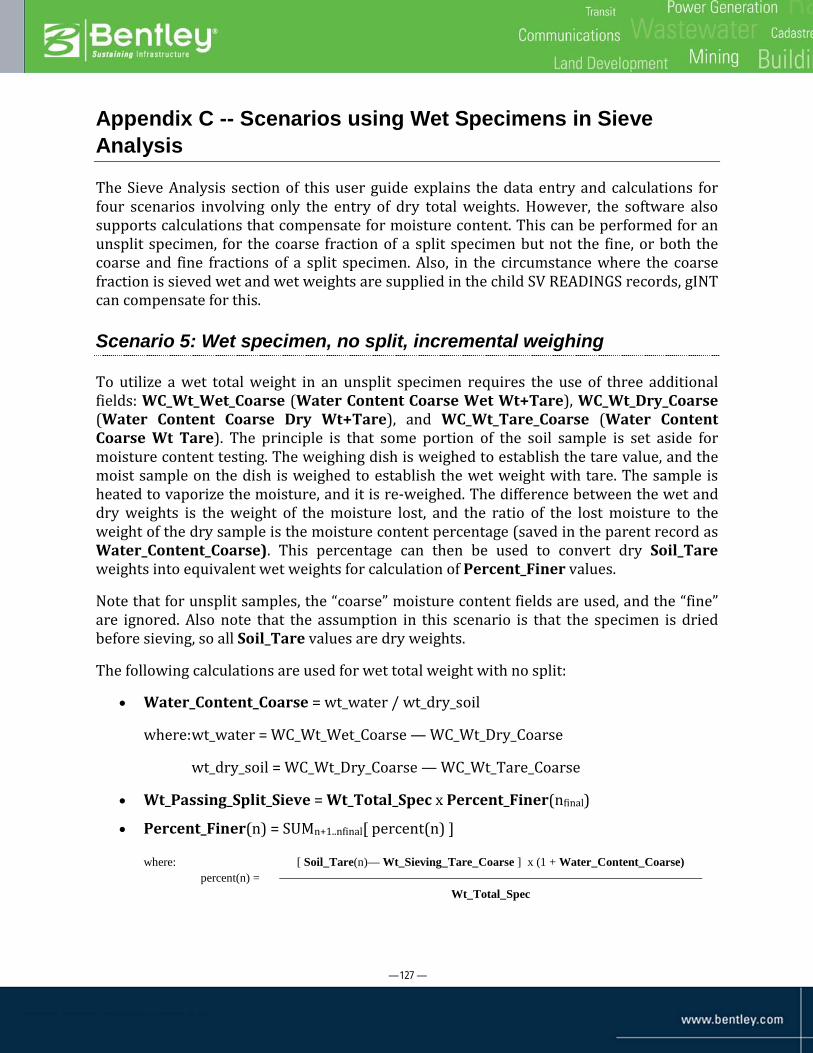
— 127 —
Appendix C -- Scenarios using Wet Specimens in Sieve Analysis
The Sieve Analysis section of this user guide explains the data entry and calculations for four scenarios involving only the entry of dry total weights. However, the software also supports calculations that compensate for moisture content. This can be performed for an unsplit specimen, for the coarse fraction of a split specimen but not the fine, or both the coarse and fine fractions of a split specimen. Also, in the circumstance where the coarse fraction is sieved wet and wet weights are supplied in the child SV READINGS records, gINT can compensate for this.
Scenario 5: Wet specimen, no split, incremental weighing
To utilize a wet total weight in an unsplit specimen requires the use of three additional fields: WC_Wt_Wet_Coarse (Water Content Coarse Wet Wt+Tare), WC_Wt_Dry_Coarse (Water Content Coarse Dry Wt+Tare), and WC_Wt_Tare_Coarse (Water Content Coarse Wt Tare). The principle is that some portion of the soil sample is set aside for moisture content testing. The weighing dish is weighed to establish the tare value, and the moist sample on the dish is weighed to establish the wet weight with tare. The sample is heated to vaporize the moisture, and it is re-weighed. The difference between the wet and dry weights is the weight of the moisture lost, and the ratio of the lost moisture to the weight of the dry sample is the moisture content percentage (saved in the parent record as Water_Content_Coarse). This percentage can then be used to convert dry Soil_Tare weights into equivalent wet weights for calculation of Percent_Finer values.
Note that for unsplit samples, the “coarse” moisture content fields are used, and the “fine” are ignored. Also note that the assumption in this scenario is that the specimen is dried before sieving, so all Soil_Tare values are dry weights.
The following calculations are used for wet total weight with no split:
• Water_Content_Coarse = wt_water / wt_dry_soil
where: wt_water = WC_Wt_Wet_Coarse — WC_Wt_Dry_Coarse
wt_dry_soil = WC_Wt_Dry_Coarse — WC_Wt_Tare_Coarse
• Wt_Passing_Split_Sieve = Wt_Total_Spec x Percent_Finer(nfinal)
• Percent_Finer(n) = SUMn+1..nfinal[ percent(n) ]
where: percent(n) =
[ Soil_Tare(n)— Wt_Sieving_Tare_Coarse ] x (1 + Water_Content_Coarse)
Wt_Total_Spec

— 128 —
Example:
We are doing an incremental calculation, no split, with moisture content, with:
ο Wt_Total_Spec = 1504
ο Wt_Sieving_Tare_Coarse = 18.4
ο WC_Wt_Wet_Coarse = 129
ο WC_Wt_Dry_Coarse = 100
ο WC_Wt_Tare_Coarse = 16.1
ο Soil_Tare values as shown in the second column of the table below.
The resulting Wt_Passing_Split_Sieve is 241.78, the Water_Content_Coarse is 34.56%, and the Percent_Finer values are as shown in the right column of the table.
Soil_Tare
(entered)
Wt_Sieving_ Tare_Coarse (entered)
net dry soil wt (calc) add wc
net wet soil wt (calc)
percent(n) (calc)
Percent_ Finer (calc)
#4 220 18.4 201.6 69.68 271.28 18.04% 81.96%
#30 225 18.4 206.6 71.41 278.01 18.48% 63.48%
#50 225 18.4 206.6 71.41 278.01 18.48% 44.99%
#100 230 18.4 211.6 73.14 284.74 18.93% 26.06%
#200 130 18.4 111.6 38.57 150.17 9.99% 16.08%
total sieved 938.00 1262.22
total specimen 1504 0.00 1504.00
wt passing split sieve
241.78 16.08%
Scenario 6: Wet specimen, split sieve
To utilize a wet split specimen requires the use of six additional fields (beyond the ones necessary for a dry split specimen):
• WC_Wt_Wet_Coarse (Water Content Coarse Wet Wt+Tare) • WC_Wt_Dry_Coarse (Water Content Coarse Dry Wt+Tare) • WC_Wt_Tare_Coarse (Water Content Coarse Wt Tare)
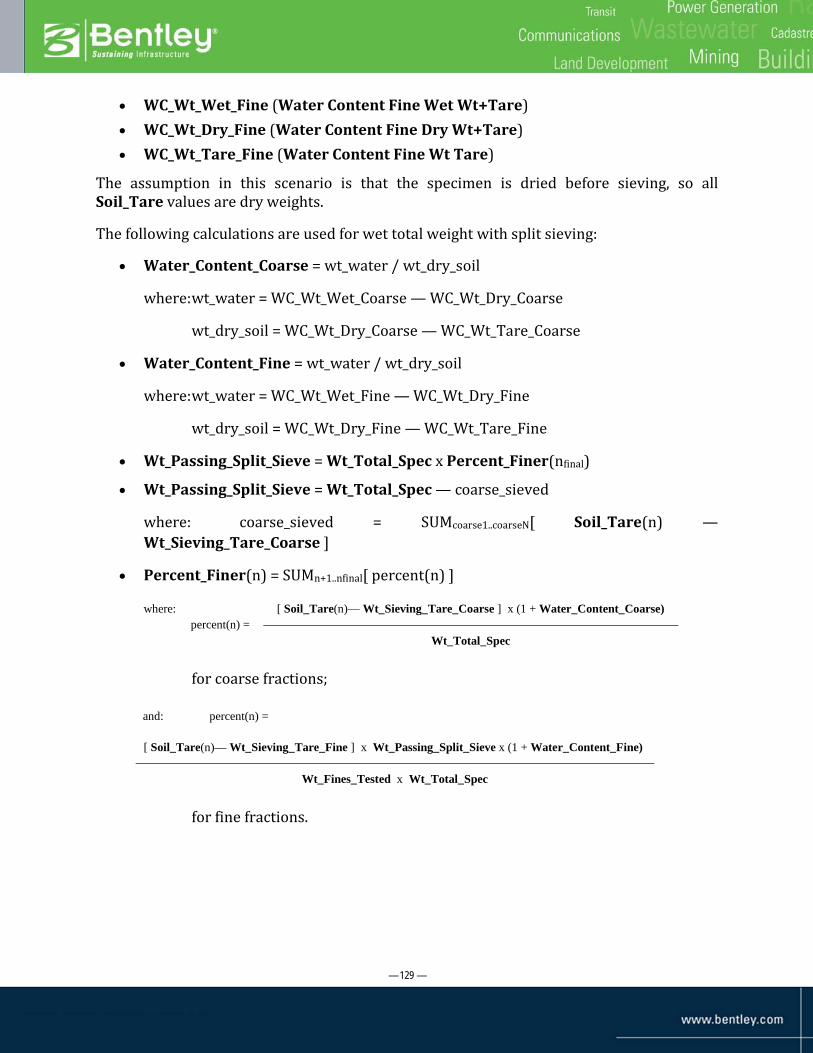
— 129 —
• WC_Wt_Wet_Fine (Water Content Fine Wet Wt+Tare) • WC_Wt_Dry_Fine (Water Content Fine Dry Wt+Tare) • WC_Wt_Tare_Fine (Water Content Fine Wt Tare)
The assumption in this scenario is that the specimen is dried before sieving, so all Soil_Tare values are dry weights.
The following calculations are used for wet total weight with split sieving:
• Water_Content_Coarse = wt_water / wt_dry_soil
where: wt_water = WC_Wt_Wet_Coarse — WC_Wt_Dry_Coarse
wt_dry_soil = WC_Wt_Dry_Coarse — WC_Wt_Tare_Coarse
• Water_Content_Fine = wt_water / wt_dry_soil
where: wt_water = WC_Wt_Wet_Fine — WC_Wt_Dry_Fine
wt_dry_soil = WC_Wt_Dry_Fine — WC_Wt_Tare_Fine
• Wt_Passing_Split_Sieve = Wt_Total_Spec x Percent_Finer(nfinal)
• Wt_Passing_Split_Sieve = Wt_Total_Spec — coarse_sieved
where: coarse_sieved = SUMcoarse1..coarseN[ Soil_Tare(n) — Wt_Sieving_Tare_Coarse ]
• Percent_Finer(n) = SUMn+1..nfinal[ percent(n) ]
where: percent(n) =
[ Soil_Tare(n)— Wt_Sieving_Tare_Coarse ] x (1 + Water_Content_Coarse)
Wt_Total_Spec
for coarse fractions;
and: percent(n) =
[ Soil_Tare(n)— Wt_Sieving_Tare_Fine ] x Wt_Passing_Split_Sieve x (1 + Water_Content_Fine)
Wt_Fines_Tested x Wt_Total_Spec
for fine fractions.

— 130 —
Example:
We are doing an incremental calculation, split sieving, with moisture content, with:
ο Wt_Total_Spec = 5201.4
ο Wt_Fines_Tested = 175
ο Size_Split_Sieve = 4.75
ο Wt_Sieving_Tare_Coarse = 28.3
ο Wt_Sieving_Tare_Fine = 18.4
ο WC_Wt_Wet_Coarse = 520.3
ο WC_Wt_Dry_Coarse = 495.8
ο WC_Wt_Tare_Coarse = 14.8
ο WC_Wt_Wet_Fine = 122.6
ο WC_Wt_Dry_Fine = 106.9
ο WC_Wt_Tare_Fine = 13.8
ο Soil_Tare values as shown in the second column of the table below.
The resulting Wt_Passing_Split_Sieve is 4805.2, the Water_Content_Coarse is 5.09%, the Water_Content_Fine is 16.86%, and the Percent_Finer values are as shown in the right column of the table.
Soil_Tare
(entered)
Wt_Sieving_ Tare_Coarse (entered)
net dry soil wt (calc) add wc
net wet soil wt (calc)
percent(n) (calc)
Percent_ Finer (calc)
3" 28.3 28.3 0 0.00 0.00 0.00% 100.00%
1-1/2" 128.4 28.3 100.1 5.10 105.20 2.02% 97.98%
3/4" 142.7 28.3 114.4 5.83 120.23 2.31% 95.67%
3/8" 123.4 28.3 95.1 4.84 99.94 1.92% 93.74%
#4 95.7 28.3 67.4 3.43 70.83 1.36% 92.38%
#8 50.8 18.4 32.4 5.46 37.86 19.99% 72.39%
#16 40.2 18.4 21.8 3.68 25.48 13.45% 58.95%
#30 35.2 18.4 16.8 2.83 19.63 10.36% 48.58%
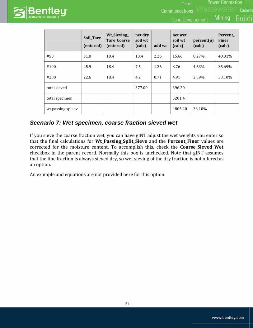
— 131 —
Soil_Tare
(entered)
Wt_Sieving_ Tare_Coarse (entered)
net dry soil wt (calc) add wc
net wet soil wt (calc)
percent(n) (calc)
Percent_ Finer (calc)
#50 31.8 18.4 13.4 2.26 15.66 8.27% 40.31%
#100 25.9 18.4 7.5 1.26 8.76 4.63% 35.69%
#200 22.6 18.4 4.2 0.71 4.91 2.59% 33.10%
total sieved 377.00 396.20
total specimen 5201.4
wt passing splt sv 4805.20 33.10%
Scenario 7: Wet specimen, coarse fraction sieved wet
If you sieve the coarse fraction wet, you can have gINT adjust the wet weights you enter so that the final calculations for Wt_Passing_Split_Sieve and the Percent_Finer values are corrected for the moisture content. To accomplish this, check the Coarse_Sieved_Wet checkbox in the parent record. Normally this box is unchecked. Note that gINT assumes that the fine fraction is always sieved dry, so wet sieving of the dry fraction is not offered as an option.
An example and equations are not provided here for this option.