Lab on a Chip

PAPER

1452 | Lab Chip, 2014, 14, 1452–1458 This journal is © The R

aDepartment of Mechanical Engineering, University of South Carolina, Columbia,

USA. E-mail: guirenwang@sc.edub Biomedical Engineering Program, University of South Carolina, Columbia, USA

† These authors have made equal contribution to this work.

Cite this: Lab Chip, 2014, 14, 1452

Received 18th December 2013,Accepted 23rd January 2014

DOI: 10.1039/c3lc51403j

www.rsc.org/loc

There can be turbulence in microfluidics at lowReynolds number

G. R. Wang,*ab Fang Yang†a and Wei Zhao†a

Turbulence is commonly viewed as a type of macroflow, where the Reynolds number (Re) has to be

sufficiently high. In microfluidics, when Re is below or on the order of 1 and fast mixing is required, so far

only chaotic flow has been reported to enhance mixing based on previous publications since turbulence is

believed not to be possible to generate in such a low Re microflow. There is even a lack of velocimeter that

can measure turbulence in microchannels. In this work, we report a direct observation of the existence of

turbulence in microfluidics with Re on the order of 1 in a pressure driven flow under electrokinetic forcing

using a novel velocimeter having ultrahigh spatiotemporal resolution. The work could provide a new

method to control flow and transport phenomena in lab-on-a-chip and a new perspective on turbulence.

1. Introduction

One important issue in microfluidics is the relatively slowmixing of two fluids due to laminar flow at low Reynoldsnumber (Re). However, in many cases, e.g. studying themechanism of protein folding which involves fast kinetics,rapid mixing is very important and highly demanded. Inmacroflows, where Re is relatively high, mixing can usuallybe enhanced by forcing flow to be turbulent. Although therecan be elastic turbulence in polymer solutions at low Re,1 itis conventionally believed that the flow in microfluidics,where typical Re is on the order of 1 or lower and thefluids are often approximately seen as Newtonian, can onlybe laminar2,3 and cannot be turbulent.4–7 There is evenno available velocimeter that can measure turbulence inmicrofluidics.8 According to a recent review, Chang andYang9 implied that, so far, many efforts have been made toenhance mixing in microfluidics, e.g. using sufficiently highDC or AC voltage to force flow in a microchannel based onelectrokinetic instability,10–15 but the forced flows in thesestudies are chaotic advection, not turbulence.

Can there be turbulence in a microchannel with Re on theorder of 1? To address this issue, we have to know first whatturbulence is. Although it is difficult to give an accuratedefinition of turbulence, there are some common features inturbulence:16 fast diffusion, random motion, high dissipationrate, continuous flow, multiscale eddies, 3-D flow and highRe. Based on these features, common knowledge is that thecritical Reynolds number—Rec—is 2100–2300 in pipe flow.

In microfluidics, turbulence is hard to be generated unlessthe pressure head is high enough.17,18 As we know, Rec inmicrochannels is similar to that in macroflows, althoughdebates exist.19 In macroflows, we have realized turbulenceand ultrafast mixing at relatively low Re based on receptivity.20,21

In the present work, we demonstrate that turbulence can beachieved in an electrokinetically forced pressure-driven flow inmicrochannels with Re on the order of 1.

2. Principle of generating andmeasuring turbulence in microfluidicsat low Re

In the present work, the principle of generating turbulence inmicrofluidics at low Re is described below. The dynamicalprocess of electrokinetics can be described by the Navier–Stokesequation as

�

� � � �utu u p u F

2

e (1)

where ρ,�u , p, η and

�Fe are the fluid density, flow velocity,

pressure, dynamic viscosity and electrical body force,

respectively.� �F Ee f , where

�E is the electric field and

f �E / denotes the initial free charge density in

solution,11 where ε is the permittivity of the electrolyte, σ is theelectric conductivity of the medium and ∇σ is the conductivitygradient. In pressure driven flows at low Re in microfluidics,usually the pressure term ∇p alone cannot surpass the viscous

force 2 �u to produce a large inertial term and generate tur-

bulence; further, the flows should be laminar. To overcome thestrong viscous force, one can introduce other body forces to

oyal Society of Chemistry 2014

Lab on a Chip Paper

balance the influence of the viscous force. In microfluidics, thiscan be realized by generating a relatively strong electric bodyforce

�Fe on the fluid. By increasing ρf through management of

the given�E and ∇σ, the ratio between the electric body force

and viscous force, i.e. the electric Grashof number Gre, can beincreased.

Gre is also the ratio of electric Rayleigh number Rae toSchmidt number Sc,22 with Rae = εw2E0

2(σ2 − σ1)/σ1ηDe andSc = η/ρDe, where De is effective diffusivity, σ1 and σ2 are theconductivities of the two streams, w is the width of the

channel at the entrance, and E V w0 2 / is the root-mean

square value of the nominal electric field strength (where V isthe applied peak-to-peak voltage between the two electrodes).Since for a given fluid, Sc is constant, Rae has been used torepresent the ratio of electrical stress to viscous forces. Thecritical Rae, beyond which the flow becomes unstable,depends on its definition and flow management and can bein the range of 10–105.23

In electrokinetics, if the inertial and electric forcesare balanced and both are larger than the viscous force,a corresponding characteristic velocity scaled by

U Ee 2 1 02/ (ref. 22) can be concluded. For a

given length scale le, we have the convective time scaleτe = le/Ue, which in turn is much smaller than the relatedviscous diffusion time τd = ρle

2/η for large le. In this case, theviscous effect is negligible compared with the convectioneffect, which due to shear stress and nonlinear effects cangenerate smaller scale structures. As le becomes smaller, τddecreases faster than τe. At sufficiently small le, where τd = τe,the viscous effect is directly balanced by the inertial andelectric effects, giving the possibly smallest length scale as

This journal is © The Royal Society of Chemistry 2014

Fig. 1 (a) Schematic of the microfluidic chip setup. The dashed arrow lindiffusion process using Laser-Induced Fluorescence. (b) Flow without forciis a dye solution. (c) Forcing under 8 Vp–p. (d) The flow becomes turbulen(e) Visualization of the flow (b) with polystyrene particles of 1 μm in diampathlines indicate that the flow is laminar. (f) The corresponding violent vor(d). The curved pathlines display the random vortices in the flow. The came

l Ede 21 0

22 1/ . Clearly if (σ2 − σ1)E0

2 is sufficiently

large, lde can be much smaller (e.g. more than one order) thanthe channel width. Hence, there could be multiple scales, afeature of turbulence. This could give the flow enough spatial-temporal space, if Rae is sufficiently high, for a continuouspower spectrum of turbulence to be developed, even thoughRe is still very low.

Previously, in electrokinetic microfluidics, the electrodesare commonly placed at the inlet and outlet of the channelto induce electrokinetic instability and increase mixing in

the flow.11,12 In such a type of micromixer, since�E is

perpendicular to ∇σ, the electric charge density ρf and the

corresponding�Fe are very small. The corresponding mixing

is achieved by amplifying the original small disturbance atthe interface between the two fluid streams due to electroki-netic instability.11 In the present work, four methods wereexplored to achieve turbulence. (1) We use two conductivesidewalls to force the flow. In this management, for a given�E and ∇σ, ρf is increased by arranging

�E to be nearly parallel

to ∇σ. In the present setup,�E is almost parallel to ∇σ, and a

strong transverse force component�F ye of

�Fe is created to

compete with the viscous force. (2) The microchannel is madeof a diffuser with a small angle to introduce a non-uniformelectric field in the x-direction, and thus, a streamwise force�F xe as well (see Fig. 1(a)). The

�F xe near the surfaces of the

two electrode are in opposite directions because of thereverse electric fields in the bulk flow direction. Synergy ofthese forces will create more local shear and a secondaryflow, which in turn can generate and enhance 3-D turbulentflow even at low Re because of incompressibility. (3) There

Lab Chip, 2014, 14, 1452–1458 | 1453

es represent the instantaneous electric field. (b–f) Visualization of theng. The top flow stream is pure buffer solution and the bottom streamt, and the diffusion is dramatically enhanced when forced at 20 Vp–p.eter. The particles are premixed only with the bottom stream. Straighttex motion of the particles with various sizes of vortices for the flow ofra exposure time was 0.1 s.

Lab on a ChipPaper

is a relatively sharp trailing edge at the entrance of themicrochannel to generate a sharp interface with high conduc-tivity gradient between the two streams. These three methodsare novel. (4) Furthermore, ∇σ is significantly enhanced byincreasing the conductivity ratio between the two streams upto 5000 : 1. This is much higher than those used in otherpublications.22,24 In addition, we also developed a velocimeterthat can measure turbulence in microfluidics.

The next challenge is how to measure and characterizeturbulent flows in microfluidics using a spatiotemporalresolved velocimeter if there is turbulence in the microchannel.Apparently there is currently no available technique thatcan measure turbulence in microfluidics.8 Well-known MicroParticle Imaging Velocimetry (μPIV)25 could have difficulty inmeasuring statistical properties of turbulence continuously at asmall flow region with high-frequency and strong fluctuations,e.g. about 1 kHz in the present work (see Fig. 4). The LaserDoppler Velocimeter (LDV)26 suffers from spatial resolution(~200 nm is required for the present study) while a hot-wireanemometer (HWA)27 is invasive and sensitive to electric fieldand difficult to use in a microchannel for point measurementaway from the walls. Other molecular tagging velocimetries28

also have low temporal resolution. To enable turbulencemeasurement in microfluidics, a velocimeter having ultrahighspatiotemporal resolution is required. Correspondingly wehave recently developed a molecular tracer based confocalsubmicroscopic and even nanoscopic velocimeter, i.e. the LaserInduced Fluorescence Photobleaching Anemometer (LIFPA)29–31

to measure the microflow velocity with unprecedentedultrahigh spatiotemporal resolution required for turbulencemeasurements. The principle of a LIFPA is given in detail inthese publications and is similar to that of a HWA, althoughthe former is a noninvasive optical method. Similar to thesingle wire of a HWA, the LIFPA mainly measures the magni-tude of velocity. Hence, if the flow is not unidirectional, themeasured signal should be the norm of two components ofvelocity, i.e. u (streamwise component) and v (transversecomponent). This will still enable us to measure turbulenceas a HWA did in its early stage. In the present work, we useour home developed confocal LIFPA to measure turbulencein microfluidics.

3. Experimental system

A schematic of the setup used for the experiment is shown inFig. 1(a). A microchannel, 240 μm in height and 130 μm inwidth at the entrance, with a total length of 5 mm was fabri-cated. The two streams from the entrance of the quasiT-channel are separated by a splitter plate and meet at itstrailing edge. The sidewalls of the channel, which have asmall divergent angle of 5°, are electrically conductive. Twostreams of fluids having fluorescent dye solution anddifferent conductivities were delivered to the microchannel.The conductivity ratio of the two streams is 5000 : 1. A func-tion generator was used to provide the AC electric signal atforcing frequency ff = 100 kHz (except the case in Fig. 6) with

1454 | Lab Chip, 2014, 14, 1452–1458

180° phase shift and various amplitudes to the two electrodesin the microchannel.

To measure the flow velocity using a LIFPA, only a smallmolecular dye solution of coumarin 102 with the sameconcentration of 20 μM was used for the two streams, giventhat there are no fluorescent particles in the flow. The dyemolecules are so small that the slip between water and dyecan be negligible, and the completely dissolved solution hasapproximately the same velocity as the dye molecules. Toobserve intuitively how fast the turbulent mixing is, visualiza-tion using a scalar dye, i.e. fluorescein sodium, was appliedand premixed only in one stream that has high conductivity.To see the existence of vortices in the flow, polystyrene micro-particles were used for visualization. The correspondingdielectrophoresis (DEP) effect on particle motion may existbut should not be the major cause of the vortex motionobserved, since the bulk velocity caused by pressure differ-ence and convection velocity generated by the electrokineticforce are relatively high. Another reason is that DEP is pro-portional to the third power of the particle diameter, and theparticle diameter used is not larger than 1 μm.

A continuous wave laser (405 nm in wave length) was usedas the excitation source. The beam was expanded and thenfocused to the detection point by an objective (PlanApo, NA1.4 oil immersions, Olympus, NY). The fluorescence signalwas captured using a photomultiplier. To reduce shot andbias noise at the high-frequency regime, suitable cut-off fre-quencies (the frequency of the low-pass filter for the currentpreamplifier) fsc are selected. The spatial resolution wasapproximately determined from the focused laser beam vol-ume that is cylindrical. The diameter and length of thisdetection volume are determined by diffraction limit and areestimated to be approximately 203 nm and 812 nm,respectively.

4. Experimental results4.1 Fast diffusion

Fig. 1 shows the fast diffusion feature without and with ACforcing, when Re (Re = UD/ν, where U, D and ν are the bulkflow velocity, the hydraulic diameter and the kinematic vis-cosity) at the entrance is 0.4 without forcing. Fig. 1(b) showsthe case without forcing. Clearly, the flow is laminar andthere is almost no mixing except for the negligible moleculardiffusion at the interface between the two streams. With forc-ing at V = 8 Vp–p, mixing is decidedly enhanced but not verydramatically, as shown in Fig. 1(c). However, at V = 20 Vp–p,the mixing becomes extraordinarily fast even near theentrance, as shown in Fig. 1(d), where the mixing is so rapidthat the visualization cannot display the correspondinglydetailed kinematic process. Apparently this indicates thatthere are relatively strong disturbances and vortex motions inthe flow, which cause large convection in the transversedirection between the two electrodes. Note that in Fig. 1(d), alittle upstream of the trailing edge, there is no mixing at all.Hence, the flow seems to undergo a sudden transition from

This journal is © The Royal Society of Chemistry 2014

Lab on a Chip Paper

laminar to turbulent motion once the two streams converge.After merely 65 μm downstream of the entrance, the concen-tration almost becomes uniform (at least on a “large scale”)in the entire y-direction. The mixing time on a large scaleunder forcing is estimated to be about 33 ms, nearly 103

times faster compared to that only by molecular diffusion inthe unforced case. Normally, such a rapid mixing onlyhappens in turbulence. Another feature of turbulence is thatthere are vortices of different scales. These vortices can alsobe visualized using polystyrene particles as tracers as shownin Fig. 1(e) and (f). The conditions are consistent withFig. 1(b) and (d), respectively. Vortices of different sizescan be clearly found in Fig. 1(f), which corresponds to theflow of Fig. 1(d).

4.2 High dissipation

A high turbulent diffusion rate is normally accompanied withhigh turbulent dissipation caused by viscous shear stresses atsmall scales. In macroflows, right beyond Rec, the turbulentdissipation (or pressure drop) will increase rapidly andnonlinearly. Since turbulent kinetic energy will be eventuallydissipated, we used the turbulent energy Te = ⟨u′s

2⟩ to repre-sent the dissipation features equivalently and qualitatively,

where u u vs 2 2 is the instantaneous velocity measured

using a LIFPA (u and v are the instantaneous velocity compo-nents in the streamwise (x) and transverse (y) directions,respectively, u′s = us − ⟨us⟩ and “⟨ ⟩” indicates ensembleaveraging). Since it is the electrokinetic force that causes theturbulence and corresponding high dissipation, the relation-ship between Te and the electric Rayleigh number (Rae =εw2E0

2(σ2 − σ1)/σ1ηDe, where w = 130 μm, ε = 7.1 × 10−10 F m−1,η = 10−3 kg m−1 s−1, De = 1.5 × 10−9 m2 s−1) is used to describethe feature of dissipation in the flow as shown in Fig. 2.As V varies from 0 Vp–p to 20 Vp–p, E0 changes from 0 to1.1 × 105 V m−1.

It can be seen that the critical value of Rae, i.e. Raec, islocated between 1.9 × 107 and 4.3 × 107, below which Teincreases slowly with a log–log slope of 0.16. However,beyond the critical point, Te increases much faster. The slope

This journal is © The Royal Society of Chemistry 2014

Fig. 2 Relationship between turbulent energy Te and Rae. Data aremeasured at y = 0, z = 0 and x3 = 100 μm.

is estimated to be about 3.03, which is 19 times larger thanthat of the laminar regime. The relationship between Te andRae is very similar to that between pressure drop and Rearound the transitional regime in macroflows. Fig. 2indicates that, in general, as Rae is increased, the forcedmicroflow also has a dramatically nonlinear increase indissipation in the turbulent flow compared with that of thelaminar flow. Fig. 2 shows the typical transition behavioraround Rae = 2.5 × 107 and a high dissipation feature ofturbulence at Rae = 4.7 × 108.

4.3 Irregularity

Another feature of turbulence is the irregularity, which canbe characterized by a time trace of velocity at a fixed spatialpoint. Time traces of us in Fig. 1(b)–(d) at x3 = 100 μm(the streamwise position is evaluated from the trailing edge)are recorded in Fig. 3. Without forcing, us is almost constant.With forcing of V = 8 Vp–p, us has small fluctuations. In thiscase, us already shows some slight irregularity, but notstrong. However, as V is further increased to 20 Vp–p, the flowpattern becomes quite different, and us is highly fluctuatedand random. Note that the forced us is much higher than theunforced one, because what the LIFPA measured directly isthe magnitude of velocity, which includes the additionalcontribution from the spanwise velocity component v.

4.4 Multiscale eddies

An intrinsic feature in turbulence is the multiscale eddiesthat can be described in the spectral space by a powerspectrum density E( f ) of us, where f is the fluctuation fre-quency of us. E( f ) without and with different V at variousstreamwise positions are given in Fig. 4. At x2 = 10 μm, withoutforcing, E( f ) is nearly flat as background noise, since there isno fluctuation of us. The reason that E( f ) at low frequency isnot completely flat could be due to the vibration of the pump.With forcing of V = 8 Vp–p, E( f ) at x2 has significantly

Lab Chip, 2014, 14, 1452–1458 | 1455

Fig. 3 Time series of us at position x3 = 100 μm, y = 0 and z = 0.Based on the measured calibration curve between flow velocity andfluorescence intensity, the measured mean velocity of us is about11.2 mm s−1, i.e. 5.3 times larger than the unforced bulk velocity U.Therefore, Re based on this forced mean us and the hydraulic diameterof the channel at x3 is about 2.

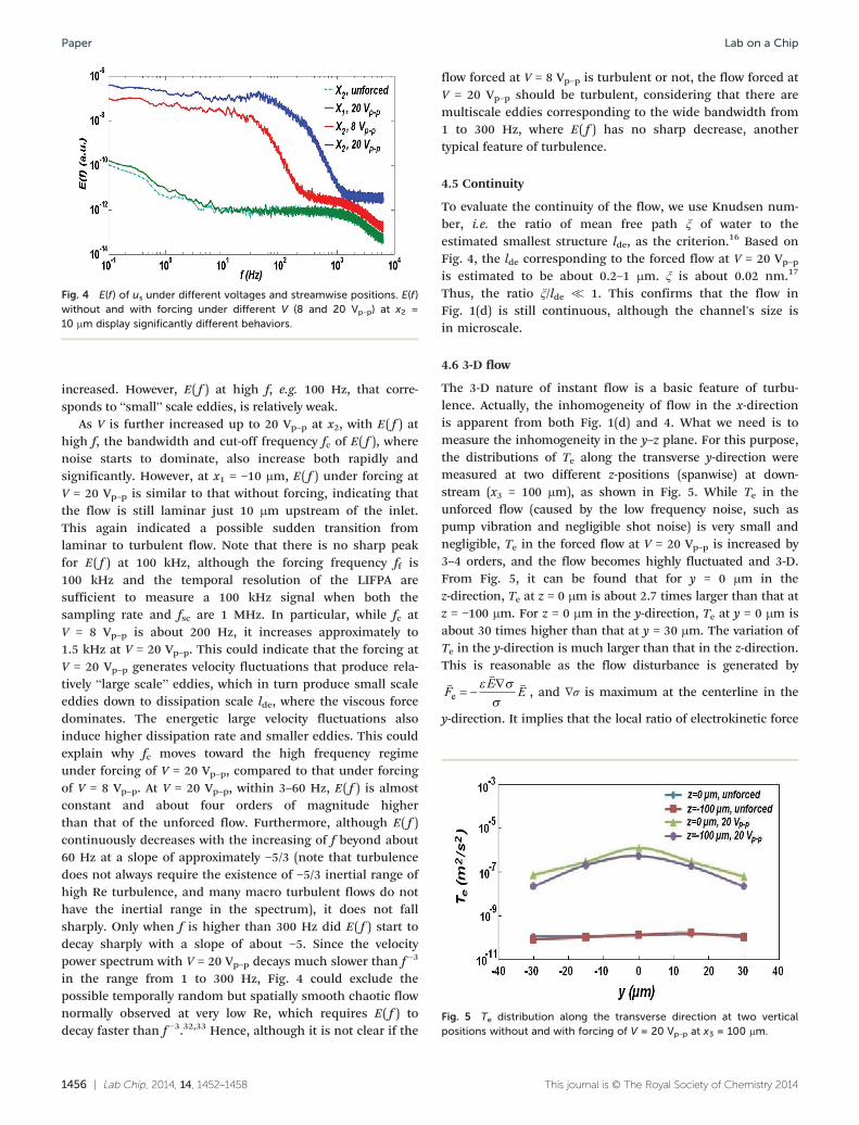
Fig. 5 Te distribution along the transverse direction at two verticalpositions without and with forcing of V = 20 Vp–p at x3 = 100 μm.

Fig. 4 E(f) of us under different voltages and streamwise positions. E(f)without and with forcing under different V (8 and 20 Vp–p) at x2 =10 μm display significantly different behaviors.

Lab on a ChipPaper

increased. However, E( f ) at high f, e.g. 100 Hz, that corre-sponds to “small” scale eddies, is relatively weak.

As V is further increased up to 20 Vp–p at x2, with E( f ) athigh f, the bandwidth and cut-off frequency fc of E( f ), wherenoise starts to dominate, also increase both rapidly andsignificantly. However, at x1 = −10 μm, E( f ) under forcing atV = 20 Vp–p is similar to that without forcing, indicating thatthe flow is still laminar just 10 μm upstream of the inlet.This again indicated a possible sudden transition fromlaminar to turbulent flow. Note that there is no sharp peakfor E( f ) at 100 kHz, although the forcing frequency ff is100 kHz and the temporal resolution of the LIFPA aresufficient to measure a 100 kHz signal when both thesampling rate and fsc are 1 MHz. In particular, while fc atV = 8 Vp–p is about 200 Hz, it increases approximately to1.5 kHz at V = 20 Vp–p. This could indicate that the forcing atV = 20 Vp–p generates velocity fluctuations that produce rela-tively “large scale” eddies, which in turn produce small scaleeddies down to dissipation scale lde, where the viscous forcedominates. The energetic large velocity fluctuations alsoinduce higher dissipation rate and smaller eddies. This couldexplain why fc moves toward the high frequency regimeunder forcing of V = 20 Vp–p, compared to that under forcingof V = 8 Vp–p. At V = 20 Vp–p, within 3–60 Hz, E( f ) is almostconstant and about four orders of magnitude higherthan that of the unforced flow. Furthermore, although E( f )continuously decreases with the increasing of f beyond about60 Hz at a slope of approximately −5/3 (note that turbulencedoes not always require the existence of −5/3 inertial range ofhigh Re turbulence, and many macro turbulent flows do nothave the inertial range in the spectrum), it does not fallsharply. Only when f is higher than 300 Hz did E( f ) start todecay sharply with a slope of about −5. Since the velocitypower spectrum with V = 20 Vp–p decays much slower than f −3

in the range from 1 to 300 Hz, Fig. 4 could exclude thepossible temporally random but spatially smooth chaotic flownormally observed at very low Re, which requires E( f ) todecay faster than f −3.32,33 Hence, although it is not clear if the

1456 | Lab Chip, 2014, 14, 1452–1458

flow forced at V = 8 Vp–p is turbulent or not, the flow forced atV = 20 Vp–p should be turbulent, considering that there aremultiscale eddies corresponding to the wide bandwidth from1 to 300 Hz, where E( f ) has no sharp decrease, anothertypical feature of turbulence.

4.5 Continuity

To evaluate the continuity of the flow, we use Knudsen num-ber, i.e. the ratio of mean free path ξ of water to theestimated smallest structure lde, as the criterion.16 Based onFig. 4, the lde corresponding to the forced flow at V = 20 Vp–p

is estimated to be about 0.2–1 μm. ξ is about 0.02 nm.17

Thus, the ratio ξ/lde ≪ 1. This confirms that the flow inFig. 1(d) is still continuous, although the channel's size isin microscale.

4.6 3-D flow

The 3-D nature of instant flow is a basic feature of turbu-lence. Actually, the inhomogeneity of flow in the x-directionis apparent from both Fig. 1(d) and 4. What we need is tomeasure the inhomogeneity in the y–z plane. For this purpose,the distributions of Te along the transverse y-direction weremeasured at two different z-positions (spanwise) at down-stream (x3 = 100 μm), as shown in Fig. 5. While Te in theunforced flow (caused by the low frequency noise, such aspump vibration and negligible shot noise) is very small andnegligible, Te in the forced flow at V = 20 Vp–p is increased by3–4 orders, and the flow becomes highly fluctuated and 3-D.From Fig. 5, it can be found that for y = 0 μm in thez-direction, Te at z = 0 μm is about 2.7 times larger than that atz = −100 μm. For z = 0 μm in the y-direction, Te at y = 0 μm isabout 30 times higher than that at y = 30 μm. The variation ofTe in the y-direction is much larger than that in the z-direction.This is reasonable as the flow disturbance is generated by�

��

F E Ee

, and ∇σ is maximum at the centerline in the

y-direction. It implies that the local ratio of electrokinetic force

This journal is © The Royal Society of Chemistry 2014

Fig. 6 E(f) with low forcing frequency of 15 Hz at position x3 = 100 μm.Compared with the unforced one, the E(f) of the forced one is muchhigher at frequency from 10 Hz to 500 Hz.

Lab on a Chip Paper

to viscosity force, i.e. Gre, changed much faster in they-direction than in the z-direction, which is due to the 3-Dvariation of conductivity structures. This indicates the intrinsic3-D nature of the flow.

5. Discussion

Since rapid time periodic forcing (100 kHz) is used to forcethe flow, it is not clear whether the large scale structures(low frequency signals) and small structures (high frequencysignal) in Fig. 4 resulted from viscous damping of muchsmaller scale structures (i.e. a much higher frequency signal),with ff = 100 kHz. If this is true, then what we have in Fig. 4could not be turbulence, but actually a chaotic flow andmixing generated in a 3-D geometry through viscous diffu-sion of the forced smaller structures produced at high ff.To address this issue, we first recall what Ottino (1990)mentioned, “It is simplistic to seek a clean answer to thequestions of whether turbulence is chaotic or chaos is turbu-lent”. We need to make it clear that studying the differencebetween chaotic flow and turbulence, a difficult topic, is outof the scope of the present work. To ensure that spectrumE( f ) in Fig. 4 with V = 20 Vp–p, including the large scale lowfrequency and small scale high frequency signals, is not justthe consequence of the viscous damping of the higherfrequency signal at such a low Re flow, we first measured theE( f ) with fsc = 1 MHz for the flow in Fig. 1(d) and found nosignal at all, but noise was detected at 100 kHz although theflow was forced at this frequency. For such a high fsc, thenoise is higher than that in Fig. 4, because shot noiseincreases with frequency.34 Then, forcing at a low ff of 15 Hzis also investigated to ensure that E( f ) has both high andlow frequency signals without high ff.

As electrolysis could create bubbles at such a low ff, wereduced the conductivity ratio to 10 and increased the forcingvoltage V to 36 Vp–p. Rae is about 2.8 × 106 in this case. Never-theless, the principle of generating turbulence in this type offlow is similar for all ff used. The result is shown in Fig. 6,

This journal is © The Royal Society of Chemistry 2014

where fc is still about 1 kHz, more than sixty times of ff.Fig. 6 indicates that the E( f ) generated at ff = 15 Hz issimilar to that at ff = 100 kHz qualitatively. The length scaleestimated from ff and bulk velocity, i.e. U/ff, is in the sameorder of the channel width. Therefore, in this case, both lowand high frequency signals in E( f ) should not be created byviscous damping of the higher frequency signal, but probablybecause of the loss of flow stability under strong forcing andturbulence. In fact, our experiment also finds that this typeof flow normally becomes more unstable at lower ff, and thelower the ff, the more unstable the flow for a given voltage.The reason we select the high frequency is mainly because ofits potential future application in lab-on-a-chip to avoid thepossible bubble generation at a low frequency.

In macroflows, low Re elastic turbulence has beenreported,1 where the fluid has to be a polymer, but no elasticturbulence has, to the best of our knowledge, been reportedin microfluidics. In the present work, the fluid is notnon-Newtonian, but common Newtonian, i.e. water solutionwith small ions. Electrokinetic forcing has also widely beenapplied in microfluidics. However, no publication hasclaimed that turbulence flow has been observed in Re below10 in electrokinetically forced flows with a Newtonian fluid.Burghelea et al.8 reported that the most popular velocimeter,μPIV, has difficulty in exploring the properties of the flowdown to sufficiently small spatial scales about its spatialstructure because of its limited resolution. Here we havenot only used a unique method to generate turbulence butalso developed a new method to be able to measure turbu-lence in microchannels. Since the origin of the transition toturbulence is not mainly because of the pressure driven pipeor channel macroflows, but the electrokinetic forcing in themicrochannel, we name the flow as micro electrokineticturbulence (or μEK turbulence) to distinguish it from “microturbulence” used already in other fields.35,36

6. Conclusion

The studied electrokinetically forced flow at sufficiently highelectric field virtually has all of the features of turbulence,which are classically used as criteria to determine if a flowis turbulent, except the Reynolds number is not high.Therefore, the present work demonstrates that increasing theelectric Rayleigh number can overcome the viscous effect togenerate turbulence, although the Reynolds number is verylow in microfluidics. This discovery may provide a newperspective on turbulence, a novel opportunity for flowmanipulation and control in microfluidics at low Re andinsight into transport phenomena in micro- and nanoscalein life science.

Acknowledgements

Weappreciate discussionswithChih-MingHo and Patrick Tabeling.The work was supported by the NSF under grant no. CAREERCBET-

Lab Chip, 2014, 14, 1452–1458 | 1457

Lab on a ChipPaper

0954977, MRI CBET-1040227 and SC EPSCOR/IDEA GEAR awardrespectively.

References1 A. Groisman and V. Steinberg, Nature, 2000, 405, 53–55.

2 A. D. Stroock, S. K. W. Dertinger, A. Ajdari, I. Mezić,

H. A. Stone and G. M. Whitesides, Science, 2002, 295,647–651.

3 D. Janasek, J. Franzke and A. Manz, Nature, 2006, 442,

374–380.

4 Y.-C. Ahn, W. Jung and Z. Chen, Lab Chip, 2008, 8, 125–133.

5 L. Capretto, W. Cheng, M. Hill and X. Zhang, Top. Curr.

Chem., 2011, 304, 42.6 C. Simonnet and A. Groisman, Phys. Rev. Lett., 2005, 94,

134501.7 S. Balasuriya, Phys. Rev. Lett., 2010, 105, 064501.

8 T. Burghelea, E. Segre, I. Bar-Joseph, A. Groisman and

V. Steinberg, Phys. Rev. E: Stat., Nonlinear, Soft Matter Phys.,2004, 69, 066305.

9 C.-C. Chang and R.-J. Yang, Microfluid. Nanofluid., 2007, 3,

501–525.

10 M. H. Oddy, J. G. Santiago and J. C. Mikkelsen, Anal. Chem.,

2001, 73, 5822–5832.

11 C.-H. Chen, H. Lin, S. K. Lele and J. G. Santiago, J. Fluid

Mech., 2005, 524, 263–303.

12 H. Hu, Z. Jin, A. Dawoud and R. Jankowiak, J. Fluid Sci.

Tech., 2008, 3, 260–273.

13 M.-Z. Huang, R.-J. Yang, C.-H. Tai, C.-H. Tsai and L.-M. Fu,

Biomed. Microdevices, 2006, 8, 309–315.

14 J. Park, S. Shin, K. Y. Huh and I. Kang, Phys. Fluids, 2005,

17, 118101.

15 H. Lin, B. D. Storey, M. H. Oddy, C.-H. Chen and

J. G. Santiago, Phys. Fluids, 2004, 16, 1922.

16 H. Tennekes and J. L. Lumley, A First Course in Turbulence,

The MIT press, 1972.

1458 | Lab Chip, 2014, 14, 1452–1458

17 B. Kirby, Micro- and Nanoscale Fluid Mechanics: Transport in

Microfluidic Devices, Cambridge University Press, 2010.

18 P. Tabeling, Introduction to Microfluidics, Oxford University

Press, USA, 2010.

19 K. V. Sharp, R. J. Adrian, J. G. Santiago and J. I. Molho, in

The Mems Handbook, ed. M. Gad-el-Hak, CRC Press, 2002.

20 G. R. Wang, AIChE J., 2006, 52, 111–124.

21 G. R. Wang, Chemical Engineering Science, 2003, 58,

4953–4963.22 J. C. Baygents and F. Baldessari, Phys. Fluids, 1998, 10, 301.

23 J. D. Posner and J. G. Santiago, J. Fluid Mech., 2006,

555, 1–42.24 A. O. El Moctar, N. Aubry and J. Batton, Lab Chip, 2003,

3, 273–280.25 J. G. Santiago, S. T. Wereley, C. D. Meinhart, D. J. Beebe and

R. J. Adrian, Exp. Fluids, 1998, 25, 316–319.26 Y. Zhao, Z. Chen, C. Saxer, S. Xiang, J. F. de Boer and

J. S. Nelson, Opt. Lett., 2000, 25, 114–116.27 C. Liu, J.-B. Huang, Z. Zhu, F. Jiang, S. Tung, Y.-C. Tai and

C.-M. Ho, J. Microelectromech. Syst., 1999, 8, 90–99.28 H. Hu and M. M. Koochesfahani, Meas. Sci. Technol.,

2006, 1269.29 C. Kuang, R. Qiao and G. Wang, Microfluid. Nanofluid., 2011,

11, 353–358.30 C. Kuang and G. Wang, Lab Chip, 2010, 10, 240–245.

31 C. Kuang, W. Zhao, F. Yang and G. Wang, Microfluid.

Nanofluid., 2009, 7, 509–517.32 A. Fouxon and V. Lebedev, Phys. Fluids, 2003, 15, 2060–2072.

33 T. Burghelea, E. Segre and V. Steinberg, Phys. Rev. Lett.,

2004, 92, 164501.34 G. R. Wang and H. E. Fiedler, Exp. Fluids, 2000, 29, 10.

35 C. D. Jager, Nature, 1954, 173, 680–681. 36 W. W. Heidbrink, J. M. Park, M. Murakami, C. C. Petty,

C. Holcomb and M. A. Van Zeeland, Phys. Rev. Lett., 2009,103, 175001.

This journal is © The Royal Society of Chemistry 2014