lab of landscape ecology and conservation biology final

Landscape Conservation Initiative • Northern Arizona University

PO Box 5694 • Flagstaff, Arizona 86011-5694

Lab of Landscape Ecology and Conservation Biology

FINAL REPORT (12 February 2015)

For the project entitled:

Implement a Rapid Plot Design across the Kaibab National Forest

USFS-NAU Agreement #14-CS-11030700-006

Submitted to:

The Kaibab National Forest

By: Valerie J. Horncastle

and

Brett G. Dickson

Recommended citation: Horncastle, V.J. and B.G. Dickson. 2015. Implement a rapid plot design across the Kaibab

National Forest. Lab of Landscape Ecology and Conservation Biology, Northern Arizona University, Flagstaff, AZ.

LLECB - Implementation of KNF Rapid Plot Design Final Report

2 | P a g e

Project overview

This report is submitted as partial fulfillment of the terms of a cost reimbursable agreement between

the Kaibab National Forest (KNF) and the Lab of Landscape Ecology and Conservation Biology at

Northern Arizona University to implement a rapid plot design (Ray et al. 2012) across the Kaibab

National Forest. Specifically, our objectives were to field test this design through plots and pilot data,

conduct summary analyses on the variables, and refine the methodology and overall plot design. The

variables in the rapid plot design were originally selected to represent several of the monitoring

components in Chapter 5 of the Kaibab National Forest Plan. We evaluated the majority of these

variables by sampling approach and effort and whether the data collected could be used to calibrate and

integrate with various remote sensed data. In addition, we discuss issues encountered in the field,

quality of the data, and provide recommendations for future rapid plot sampling efforts.

From June 2 to August 15, 2014, all 3 Kaibab National Forest Ranger Districts were visited and a total

of 291 rapid plots were sampled (Williams = 118, Tusayan = 71, North Kaibab = 102) (Figures 1 and 2).

The Tusayan Ranger District was 90% completed with only 8 plots not visited due to issues with access

(e.g., due to closed or impassable roads). We completed 80% of the Williams Ranger District and 65% of

the North Kaibab Ranger District. The majority of plots not visited in the Williams Ranger District were

because of closures due to the Sitgreaves Complex fire and other road closure types, causing the

sampling of some plots to be impractical or impossible.

There were about 10-15 occasions when prospective plots needed to be moved because they were

either located on a road or were located where slopes were > 15% (as designated in the sampling

protocol). Plots were always relocated within the same vegetation type and only moved the minimum

distance necessary to locate the plot away from an open road (typically, 20-30 m).

Although there were only 6 vegetation categories identified on the original data sheet, dominant

vegetation type(s) observed at each plot were placed into 13 unique categories (Table 1). We added

sagebrush and scrub types, and the majority of other new classifications were due to some plots having

a ~ 50/50 mix of two dominant vegetation types. In these cases, the two types were lumped into a new

single category (e.g., ‘ponderosa pine, oak’). For future syntheses and analyses, these 13 categories

could easily be reduced to a smaller set, as needed.

As expected, several rapid plots were located within planned 4FRI treatment areas and other

designated treatments throughout the Williams and Tusayan Ranger Districts. Within the Williams

Ranger District, there were 29 plots sampled within planned 4FRI treatment areas and 3 plots in other

designated treatment areas. In the Tusayan Ranger District, 14 rapid plots were located in 4FRI planned


3 | P a g e

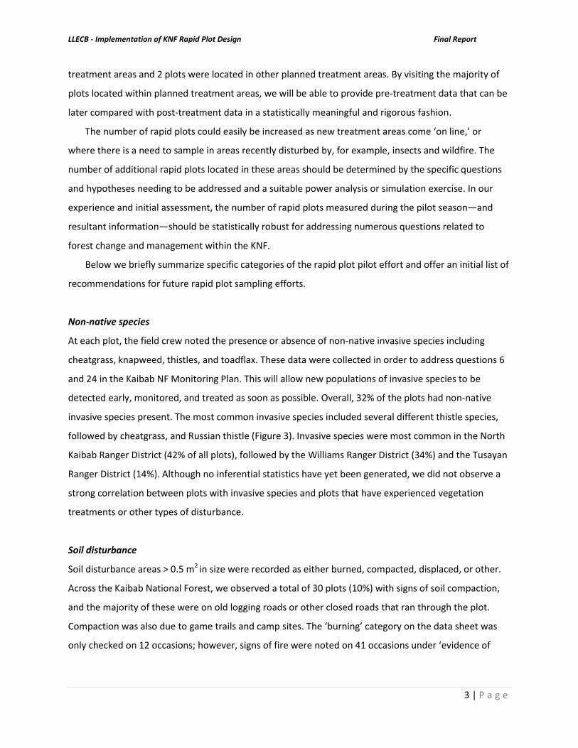
treatment areas and 2 plots were located in other planned treatment areas. By visiting the majority of

plots located within planned treatment areas, we will be able to provide pre-treatment data that can be

later compared with post-treatment data in a statistically meaningful and rigorous fashion.

The number of rapid plots could easily be increased as new treatment areas come ‘on line,’ or

where there is a need to sample in areas recently disturbed by, for example, insects and wildfire. The

number of additional rapid plots located in these areas should be determined by the specific questions

and hypotheses needing to be addressed and a suitable power analysis or simulation exercise. In our

experience and initial assessment, the number of rapid plots measured during the pilot season—and

resultant information—should be statistically robust for addressing numerous questions related to

forest change and management within the KNF.

Below we briefly summarize specific categories of the rapid plot pilot effort and offer an initial list of

recommendations for future rapid plot sampling efforts.

Non-native species

At each plot, the field crew noted the presence or absence of non-native invasive species including

cheatgrass, knapweed, thistles, and toadflax. These data were collected in order to address questions 6

and 24 in the Kaibab NF Monitoring Plan. This will allow new populations of invasive species to be

detected early, monitored, and treated as soon as possible. Overall, 32% of the plots had non-native

invasive species present. The most common invasive species included several different thistle species,

followed by cheatgrass, and Russian thistle (Figure 3). Invasive species were most common in the North

Kaibab Ranger District (42% of all plots), followed by the Williams Ranger District (34%) and the Tusayan

Ranger District (14%). Although no inferential statistics have yet been generated, we did not observe a

strong correlation between plots with invasive species and plots that have experienced vegetation

treatments or other types of disturbance.

Soil disturbance

Soil disturbance areas > 0.5 m2 in size were recorded as either burned, compacted, displaced, or other.

Across the Kaibab National Forest, we observed a total of 30 plots (10%) with signs of soil compaction,

and the majority of these were on old logging roads or other closed roads that ran through the plot.

Compaction was also due to game trails and camp sites. The ‘burning’ category on the data sheet was

only checked on 12 occasions; however, signs of fire were noted on 41 occasions under ‘evidence of


4 | P a g e

disturbance.’ Overall, soil disturbance due to fires was observed at 42 plots (14%).

Evidence of treatment or disturbance

Across all plots, only 17% of the plot locations were associated with evidence of treatments. Treatments

were marked as either commercial, lop and scatter, thin and burn, or just thinned if more specifics were

not identifiable. Whenever possible, treatments were classified as either ‘recent’ or ‘old.’ Fourteen plots

were classified as lop and scatter, 15 as commercial, 2 as burn treatments, 1 as thinned and burned, and

the other 18 plots showed evidence of thinning, but could not be classified as a particular type of

treatment. Sixteen percent of the plots had evidence of some type of disturbance. Disturbances were

indicated as low intensity burns (9 plots; likely due to treatment activities), hot burns (6), wildfires in

general (25), wind throw (3), heavy grazing (1), or heavy erosion (1).

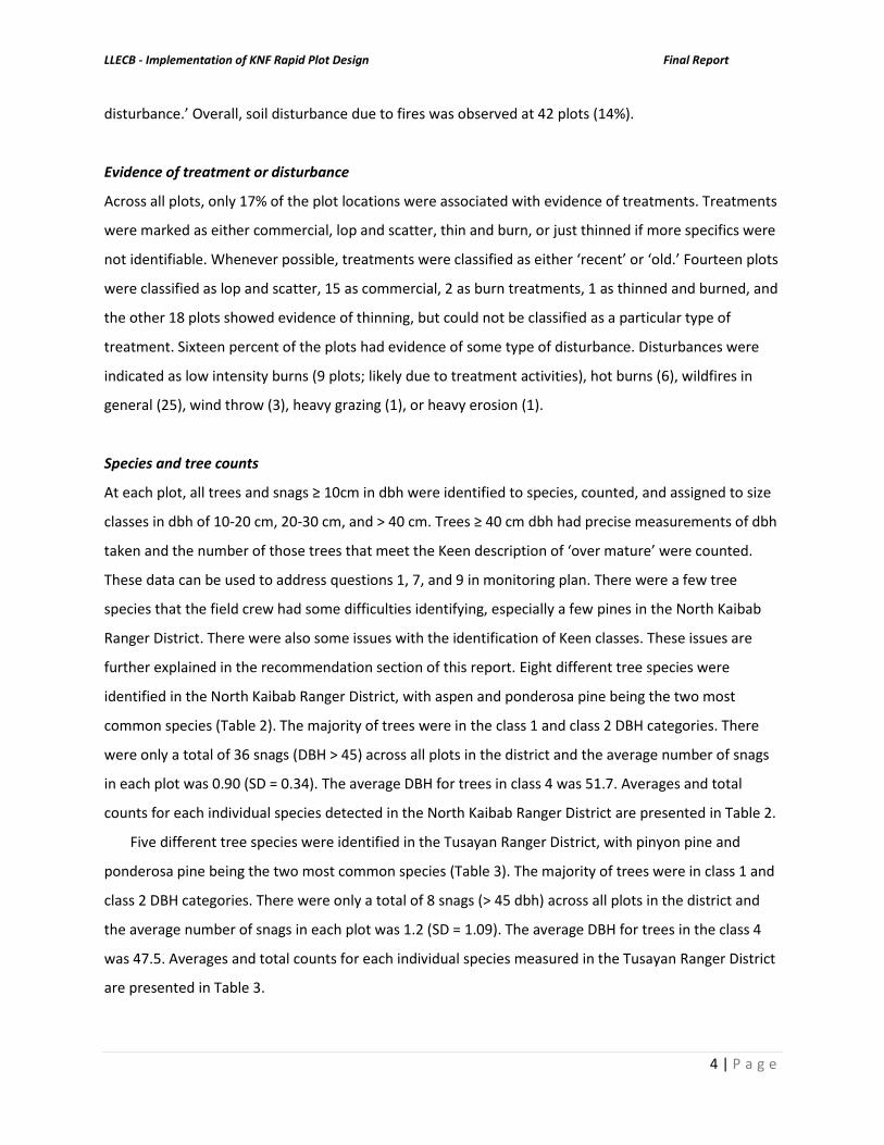
Species and tree counts

At each plot, all trees and snags ≥ 10cm in dbh were identified to species, counted, and assigned to size

classes in dbh of 10-20 cm, 20-30 cm, and > 40 cm. Trees ≥ 40 cm dbh had precise measurements of dbh

taken and the number of those trees that meet the Keen description of ‘over mature’ were counted.

These data can be used to address questions 1, 7, and 9 in monitoring plan. There were a few tree

species that the field crew had some difficulties identifying, especially a few pines in the North Kaibab

Ranger District. There were also some issues with the identification of Keen classes. These issues are

further explained in the recommendation section of this report. Eight different tree species were

identified in the North Kaibab Ranger District, with aspen and ponderosa pine being the two most

common species (Table 2). The majority of trees were in the class 1 and class 2 DBH categories. There

were only a total of 36 snags (DBH > 45) across all plots in the district and the average number of snags

in each plot was 0.90 (SD = 0.34). The average DBH for trees in class 4 was 51.7. Averages and total

counts for each individual species detected in the North Kaibab Ranger District are presented in Table 2.

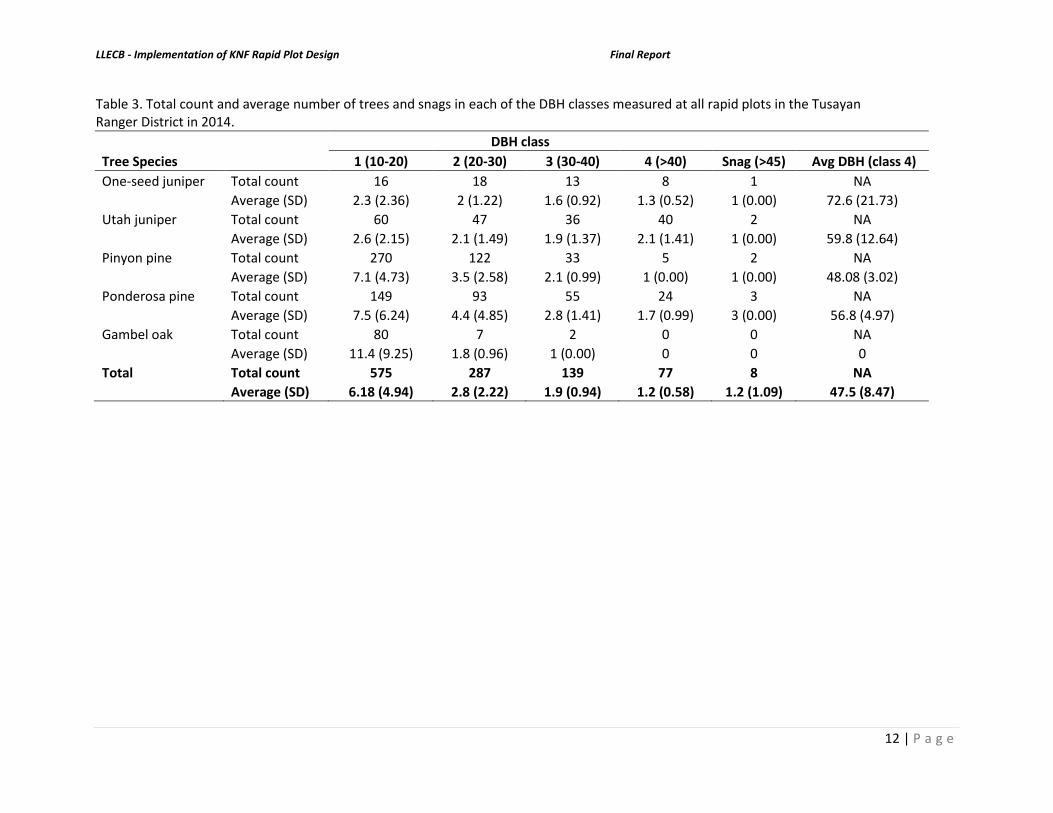
Five different tree species were identified in the Tusayan Ranger District, with pinyon pine and

ponderosa pine being the two most common species (Table 3). The majority of trees were in class 1 and

class 2 DBH categories. There were only a total of 8 snags (> 45 dbh) across all plots in the district and

the average number of snags in each plot was 1.2 (SD = 1.09). The average DBH for trees in the class 4

was 47.5. Averages and total counts for each individual species measured in the Tusayan Ranger District

are presented in Table 3.


5 | P a g e

Ten different tree species were identified in the Williams Ranger District with ponderosa pine, Utah

juniper, and Gambel oak being the most common species (Table 4). The majority of trees were in class 1

and class 2 DBH categories. There were only a total of 15 snags (> 45 dbh) across all plots in the district

and the average number of snags in each plot was 0.9 (SD = 0.06). The average DBH for trees in the class

4 was 55.7. Averages and total counts for each individual species detected in the Williams Ranger

District are presented in Table 4.

Woody debris

Coarse woody debris was measured using an adaptation of the line intersect method for forest fuels

(van Wagner 1968) using the two main transects in the plot. All logs > 8cm diameter were measured at

the point they intersected the transects. Length measurements, diameter, and decay class were noted

for each log. This information can be used to address questions 1 and 2 of the Kaibab monitoring plan.

Across the Kaibab National Forest, woody debris occurred in 55% of the plots sampled. The maximum

amount of woody debris in a plot was 39 logs. The average was 5.7 logs per plot (SD = 6.6, mode = 1.0).

North Kaibab plots exhibited the largest amount of woody debris (70.6% of all plots), while the Williams

(47.5%) and Tusayan (46.5%) Ranger Districts were similar in the proportion of plots with down logs.

Plots with the highest amounts of woody debris typically occurred in the aspen or mixed conifer

dominated vegetation type categories.

Photo plots and fuels analysis

At each plot, a photo of the plot was taken from the southern end of the north-south transect.

Additionally, photos of 1m2 quadrants were taken 2.5 m from the plot center along each of the 4

transect lines. These photos can be used for estimating fine fuels at each plot using the PHOTOLOAD

technique (Keane and Dickson 2007). Although it was beyond the scope of this project to analyze these

photos, it only took about 30 seconds to take all 5 pictures at each plot. Continuing the collection of

these photos should allow for quick estimates of fuel loadings with little time spent out in the field. The

PHOTOLOAD data along with coarse woody debris and litter and duff depths can provide a

comprehensive depiction of fuel loading within the plot and relates directly to question 8 in the

monitoring plan.

Comparing rapid plots to digitally derived estimates of forest structure


6 | P a g e

To explore relations between field data and digital data layers used to estimate key forest structure

attributes across the Kaibab National Forest (KNF), we used a GIS to intersect each rapid plot location

with data layers derived using Forest Inventory and Analysis (FIA) plot data and Landsat imagery

acquired in 2010 (see Dickson et al. 2011). Specifically, we intersected rapid plots with layers describing

basal area (BA), canopy cover (CC), height, trees per acre (TPA), stand density index (SDI), and quadratic

mean diameter (QMD) (Appendix A). For comparison, we used information collected at each rapid plot

location to estimate BA, QMD, TPA and SDI. Importantly, canopy cover (i.e., closure) and tree height

were not measured at rapid plots so we were unable to compare these metrics. Since individual trees <

40 cm DBH were not measured at rapid plots, we used size classes (as reported on data sheets: 10-20,

20-30, 30-40) to estimate QMD, BA, and SDI. For example, in each size class, we used the average value

of the classification range (e.g., a 15 cm DBH was used for a tree in the 10-20 cm DBH class). Notably, a

lack of individual tree measurements presented a challenge when trying to make comparisons with the

derived data layers, or even FIA data directly. We converted DBH cm to inches before making our

calculations. Using the rapid plot data, TPA and SDI were calculated two different ways. The first

calculation (TPA1 and SDI1) only accounted for trees greater than 3.94” DBH (10 cm DBH), while the

second calculation (TPA2 and SDI2) included both saplings and seedlings. Data collected in the field

combined seedling and sapling counts into one group so we were unable to separate these counts. This

led to sometimes very high TPA and SDI values, since some of the plots had > 100 saplings in a plot. The

digital structure data, however, included FIA-measured trees > 1” DBH in the calculations. Thus, values

for TPA1 or TPA2 were consistently lower or higher, respectively, than the derived estimates, especially

for rapid plots with a large number of seedlings. We used English units for all calculations.

We used a Pearson correlation coefficient to compare (using English units) the rapid plot and

digital structure data for QMD, TPA, BA, and SDI. Correlation coefficients were greater when comparing

TPA1 and SDI1 to digital data than for TPA2 and SDI2. Therefore we used TPA1 and SDI1 to evaluate and

summarize our results. SDI had the highest correlation coefficient with a value of 0.71, followed by BA

(0.69), TPA (0.61), and QMD at 0.44.

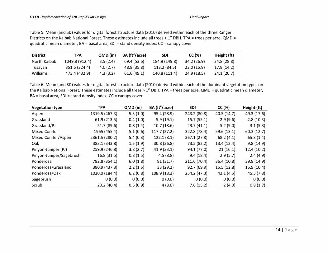
For each of the three Ranger Districts (RD) and each of the dominant vegetation types (classified

by technicians at each plot), we calculated the mean and standard deviation of TPA, BA, SDI, and QMD

using the forest structure data (Tables 5 and 6) and information collected at all rapid plot locations

(Tables 7 and 8). For both datasets, mean TPA, BA, and SDI were highest in the North Kaibab RD,

followed by the Williams RD and then the Tusayan RD. Mean QMD, however, was highest in the

Williams RD and lowest in the North Kaibab RD. The mixed conifer, mixed conifer/aspen, and


7 | P a g e

ponderosa/oak vegetation types tended to have the largest mean values for TPA, BA, SDI, and QMD,

based on both the rapid plot data and the digital forest structure data layers.

Time and cost

Our field crew of two averaged about 26-28 plots per week. Each plot, on average, took 45-60 minutes

to complete. Grassland-dominated plots were completed the quickest, taking an average of 15-20

minutes, followed by ponderosa pine and oak-dominated plots (30-40 minutes) and mixed conifer plots

(30-70 minutes). The amount of down logs at a plot contributed to the wide variability in time to

complete a plot, since they added a significant amount of extra time. Due to the variability in time to

complete plots and the difference in mileage from Flagstaff to the different Ranger Districts, the cost per

plot also varied. An approximate average cost of a plot was about $68. This average was based on a

weekly cost divided by the number of plots completed in that week and includes supplies, 2 technician

salaries, rental vehicle, gas, and per diem. If a rental vehicle was not needed, the average cost could

probably drop to ~ $58/plot.

Considering the aforementioned calculations, comparisons, and challenges, we recommend the

following changes be considered in any adjustment to the rapid plot data collection protocols.

Recommendations and clarification for future rapid plot sampling efforts

Reevaluate vegetation type categories

We increased the number of possible vegetation type categories over the number that was

indicated on the original draft data sheet. This was because several plots had a mix of two

vegetation types. A total number of meaningful categories should be reconsidered prior to

future sampling efforts.

Include sagebrush/scrub as a unique vegetation category

Several of the plots that were initially listed as grassland in the selection of plots were actually

sagebrush or scrub dominated.

For the point-line intercepts, we classified logs as litter, but this may not be desirable in future

sampling efforts.

MVUM roads should be used in the future for selecting new points along with private land.

There were several plots that were not sampled due to private property or closed or non-

existent roads.


8 | P a g e

Development of better field guides (plant identification, Keen class descriptions, invasive species)

The field crew did have some problems distinguishing between Utah and one-seed juniper

species, and between white fir and subalpine fir. For these and other similar species, we

recommend having better field guides/plant identification guides available for field crews to

keep while out in the field.

The categories that indicated maturity (platy, yellow, furrowed, or sloughing bark of old trees

and Keen Class 4 trees) were rarely marked on the data sheet. This was probably due to some

confusion about what these categories actually mean. It would be a good idea to provide more

information on these categories and how these data will be used so future crews have a better

understanding of how to apply the categorization. A reference sheet with color photos showing

trees that would be classified as Keen/Dunning (play yellow bark, etc.) and larger older trees

that do not fit into the Keen/Dunning classification would be more useful than just having the

line drawings. The 2014 crew was also unsure about whether these data should be collected

only in the ponderosa pine-dominated vegetation type, or in other conifer species as well.

Provide maps with known treatment areas and wildfire locations

It was difficult to distinguish between burning treatment and wildfires unless it was a very hot

burn or a very recent thin and burn treatment. Thus, most fire evidence was noted in the

‘disturbance’ category even if it appeared to be a light burn. Noting fire presence in the field is

useful but it would probably be wise to compare these observations to maps of known

treatment areas and wildfire locations.

Provide better clarification on overtopping and encroachment

Overtopping and encroachment were only noted at two plots. Glancing through the raw data it

appears that this was actually occurring more often than was documented. For example, if there

were a lot of new young trees invading what was a grassland or aspen stand, then this pattern

should be reflected in the belt transects and in some of the tree count data. Reviewing the data

in this way, however, will take longer than just having it properly marked on the data sheets. For

future field efforts, clarification should be provided for these categories, as well as noting to the

field crew the importance of encroachment.

Reevaluate the inclusion of canopy closure measurements

Forest canopy greatly influences microhabitat within the forest by affecting plant growth and

survival. Collecting this information would provide additional vegetation and wildlife habitat


9 | P a g e

information and would also allow for additional comparisons and calibrations to other data sets,

such as FIA data or digital data layers that estimate canopy condition. Since, the addition of a

canopy closure measurement to the rapid plot protocol would add several minutes to the time

spent per plot, the KNF might consider using ‘off the shelf’ estimates of canopy cover (e.g.,

obtained from the LANDFIRE program or the National Land Cover Database).

Separate out sapling counts by > 1” DBH and those < 1” DBH

If the KNF is interested in more precise comparisons between rapid plot data and FIA data or

digital data layers, we recommend separating out sapling and seedlings by using a 1” DBH cut

point. This distinction between saplings and seedlings would probably add an additional 2

minutes to the time spent per plot. To offset the additional time it would take to separate

counts by these two size classes, the number of transects could potentially be cut in half (2

transects instead of 4), and we recommend testing this option in the field.

Measure all trees > 4” DBH and do not use size classes

A precise DBH measurement of all individual trees within rapid plots > 4" DBH would allow for

more reasonable, integrated measurements of forest structure attributes, such as stand BA or

QMD. More precise measurements would also allow for better calibration of the remotely

sensed data. The additional time for these measurements would vary greatly by plot and

vegetation type, but shouldn’t take more than 5 minutes. Since this approach would be more

time consuming, another option would be to measure all trees > 8” DBH and place smaller trees

into bin categories. This would reduce the amount of time in the field but still provide more

precise measurements since the larger trees contribute more to basal area calculations. Future

work might involve conducting a sensitivity analysis to determine which cutoff size produces

more accurate results, without adding too much additional time to full implementation of the

rapid plot protocol.


10 | P a g e

Table 1. Number of rapid plots sampled during the 2014 field season in each of the 13

dominant vegetation type categories we considered, and across the three Kaibab

National Forest Ranger Districts. PJ = pinyon-juniper.

Vegetation type North Kaibab Tusayan Williams Grand Total

Aspen 5 0 2 7

Aspen, Mixed Conifer 6 0 0 6

Grassland 10 7 22 39

Grassland, PJ 0 2 1 3

Mixed Conifer 28 0 2 30

Oak 8 0 1 9

PJ 14 34 37 85

PJ, Sagebrush 3 3 0 6

Ponderosa 21 22 46 89

Ponderosa, Grassland 0 1 1 2

Ponderosa, Oak 0 0 5 5

Sagebrush 4 2 0 6

Scrub 3 0 1 4

Grand Total 102 71 118 291


11 | P a g e

Table 2. Total count and average number of trees and snags in each of the DBH classes measured at all rapid plots in the North Kaibab Ranger District in 2014. * indicates trees that could only be identified to the Pinus genera.

DBH class

Tree Species 1 (10-20) 2 (20-30) 3 (30-40) 4 (>40) Snag (>45) Avg. DBH (class 4)

Subalpine fir Total count 48 21 12 2 2 NA

Average (SD) 4 (2.86) 2.6 (1.99) 2 (1.09) 1 (0.00) 1 (0.00) 48.2 (0.98)

White fir Total count 84 13 11 6 0 NA

Average (SD) 4.2 (4.6) 1.4 (0.73) 1.8 (1.6) 1.5 (1.0) 0 50.5 (2.35)

Utah juniper Total count 30 22 28 25 3 NA

Douglas fir Total count 105 63 55 38 5 NA

Average (SD) 4.2 (4.28) 2.7 (2.45) 2.6 (1.98) 2.0 (1.00) 1 (0.00) 51.4 (5.82)

Average (SD) 2.7 (1.95) 2 (1.0) 2.2 (1.28) 2.5 (1.35) 1 (0.00) 59 (8.21)

Pinyon pine Total count 103 35 11 2 0 NA

Average (SD) 8.6 (10.66) 4.4 (3.46) 1.8 (1.17) 1 (0.0) 0 44.6 (0.57)

Ponderosa pine Total count 190 88 60 100 15 NA

Average (SD) 6.5 (8.3) 3.8 (4.42) 2.5 (1.77) 2.9 (2.2) 1.4 (0.67) 55.9 (7.73)

Pinus spp.* Total count 99 29 28 17 3 NA

Average (SD) 3.5 (3.14) 1.8 (1.32) 2.3 (2.02) 1.4 (0.51) 1.5 (0.71) 53.8 (5.27)

Aspen Total count 345 77 35 12 8 NA

Average (SD) 10.5 (12.34) 2.9 (2.29) 2.1 (1.02) 2 (2.00) 1.6 (1.34) 50.2 (4.23)

Gambel oak Total count 8 1 0 0 0 NA

Average (SD) 8 (0.00) 1 (0.00) 0 0 0 0

Total Total count 1012 349 240 202 36 NA

Average (SD) 5.5 (6.01) 2.7 (2.21) 2.2 (1.49) 1.8 (1.00) 0.9 (0.34) 51.7 (4.39)


12 | P a g e

Table 3. Total count and average number of trees and snags in each of the DBH classes measured at all rapid plots in the Tusayan Ranger District in 2014.

DBH class

Tree Species 1 (10-20) 2 (20-30) 3 (30-40) 4 (>40) Snag (>45) Avg DBH (class 4)

One-seed juniper Total count 16 18 13 8 1 NA

Average (SD) 2.3 (2.36) 2 (1.22) 1.6 (0.92) 1.3 (0.52) 1 (0.00) 72.6 (21.73)


Average (SD) 2.6 (2.15) 2.1 (1.49) 1.9 (1.37) 2.1 (1.41) 1 (0.00) 59.8 (12.64)


Average (SD) 7.1 (4.73) 3.5 (2.58) 2.1 (0.99) 1 (0.00) 1 (0.00) 48.08 (3.02)


Average (SD) 7.5 (6.24) 4.4 (4.85) 2.8 (1.41) 1.7 (0.99) 3 (0.00) 56.8 (4.97)


Average (SD) 11.4 (9.25) 1.8 (0.96) 1 (0.00) 0 0 0


Average (SD) 6.18 (4.94) 2.8 (2.22) 1.9 (0.94) 1.2 (0.58) 1.2 (1.09) 47.5 (8.47)


13 | P a g e

Table 4. Total count and average number of trees and snags in each of the DBH classes measured at all rapid plots in the Williams Ranger District in 2014.

DBH class

Tree Species 1 (10-20) 2 (20-30) 3 (30-40) 4 (>40) Snag (>45) Avg DBH (class 4)

White fir Total count 0 0 2 1 0 NA

Average (SD) 0 0 2 (0.00) 1 (0.00) 0 56

Douglas fir Total count 11 8 5 4 5 NA

Average (SD) 5.5 (0.71) 4 (1.41) 2.5 (0.71) 2 (1.41) 5 (0.00) 51.4 (3.51)

Alligator juniper Total count 68 32 26 31 0 NA

Average (SD) 3.1 (2.74) 1.8 (0.94) 1.6 (0.96) 2.1 (1.53) 0 65.6 (16.97)

One-seed juniper Total count 22 26 23 26 0 NA

Average (SD) 2.8 (1.75) 2.6 (2.8) 2.3 (2.31) 3.7 (2.69) 0 55.8 (9.89)


Average (SD) 4.0 (3.17) 3.3 (2.33) 2.6 (2.10) 2.4 (1.54) 1 (0.00) 61.3 (13.56)


Average (SD) 2.6 (1.86) 1.6 (1.24) 1.3 (0.82) 0 1 (0.00) 0


Average (SD) 5.4 (4.79) 4.2 (4.5) 3.6 (2.59) 2.4 (1.65) 1.2 (0.41) 48.9 (5.85)

White pine Total count 7 1 2 3 0 NA

Average (SD) 7 (0.00) 1 (0.00) 2 (0.00) 3 (0.00) 0 44.9 (2.38)

Aspen Total count 36 4 2 0 0 NA

Average (SD) 18 (12.73) 2 (1.41) 2 (0.00) 0 0 0


Average (SD) 7.7 (7.01) 4.7 (4.23) 2.4 (2.51) 2.3 (1.58) 0 50.9 (9.99)


Average (SD) 5.4 (4.34) 2.7 (2.35) 2.3 (1.49) 1.8 (1.49) 0.9 (0.06) 55.7 (9.96)


14 | P a g e

Table 5. Mean (and SD) values for digital forest structure data (2010) derived within each of the three Ranger Districts on the Kaibab National Forest. These estimates include all trees > 1” DBH. TPA = trees per acre, QMD = quadratic mean diameter, BA = basal area, SDI = stand density index, CC = canopy cover

District TPA QMD (in) BA (ft2/acre) SDI CC (%) Height (ft)

North Kaibab 1049.8 (912.4) 3.5 (2.4) 69.4 (53.6) 184.9 (149.8) 34.2 (26.9) 34.8 (28.8)

Tusayan 351.5 (324.4) 4.0 (2.7) 48.9 (35.8) 113.2 (84.5) 23.0 (15.9) 17.9 (14.2)

Williams 473.4 (432.9) 4.3 (3.2) 61.6 (49.1) 140.8 (111.4) 24.9 (18.5) 24.1 (20.7)

Table 6. Mean (and SD) values for digital forest structure data (2010) derived within each of the dominant vegetation types on the Kaibab National Forest. These estimates include all trees > 1” DBH. TPA = trees per acre, QMD = quadratic mean diameter, BA = basal area, SDI = stand density index, CC = canopy cover

Vegetation type TPA QMD (in) BA (ft2/acre) SDI CC (%) Height (ft)

Aspen 1319.5 (467.3) 5.3 (1.0) 95.4 (28.9) 243.2 (80.8) 40.5 (14.7) 49.3 (17.6)

Grassland 61.9 (213.5) 0.4 (1.0) 5.9 (19.1) 15.7 (55.1) 2.9 (9.6) 2.8 (10.3)

Grassland/PJ 51.7 (89.6) 0.8 (1.4) 10.7 (18.6) 23.7 (41.1) 5.2 (9.0) 3.1 (5.3)

Mixed Conifer 1965 (455.4) 5.1 (0.6) 117.7 (27.2) 322.8 (78.4) 59.6 (13.1) 60.3 (12.7)

Mixed Conifer/Aspen 2361.5 (280.2) 5.4 (0.3) 122.1 (8.1) 367.1 (27.8) 68.2 (4.1) 65.3 (1.4)

Oak 383.1 (343.8) 1.5 (1.9) 30.8 (36.8) 73.5 (82.2) 13.4 (12.4) 9.8 (14.9)

Pinyon-Juniper (PJ) 259.9 (246.8) 3.8 (2.7) 41.9 (33.1) 94.1 (77.0) 21 (16.1) 12.4 (10.2)

Pinyon-Juniper/Sagebrush 16.8 (31.5) 0.8 (1.5) 4.5 (8.8) 9.4 (18.4) 2.9 (5.7) 2.4 (4.9)

Ponderosa 782.8 (354.1) 6.0 (1.8) 91 (31.7) 211.6 (70.4) 36.4 (10.8) 39.8 (14.9)

Ponderosa/Grassland 380.9 (437.3) 2.2 (1.5) 33 (29.2) 92.7 (69.9) 15.5 (12.8) 15.9 (10.4)

Ponderosa/Oak 1030.0 (184.4) 6.2 (0.8) 108.9 (18.2) 254.2 (47.3) 42.1 (4.5) 45.3 (7.8)

Sagebrush 0 (0.0) 0 (0.0) 0 (0.0) 0 (0.0) 0 (0.0) 0 (0.0)

Scrub 20.2 (40.4) 0.5 (0.9) 4 (8.0) 7.6 (15.2) 2 (4.0) 0.8 (1.7)


15 | P a g e

Table 7. Mean (and SD) values for rapid plot data collected during 2014 within each of the three Ranger Districts on the Kaibab National Forest. QMD and BA were calculated using the mean of the DBH class ranges and TPA1 and SDI1 were calculated using trees > 3.94” DBH. TPA = trees per acre, QMD = quadratic mean diameter, BA = basal area, SDI = stand density index

District TPA1 QMD (in) BA (ft2/acre) SDI1

North Kaibab 103.2 (92.3) 9.7 (6.5) 68.7 (56.1) 118.4 (95.0)

Tusayan 87.7 (70.4) 9.9 (4.5) 52.5 (40.1) 92.7 (68.3)

Williams 82.8 (72.8) 10.5 (5.3) 65.3 (51.6) 109.6 (85.6)

Table 8. Mean (and SD) values for rapid plot data collected during 2014 within each of the dominant vegetation types on the Kaibab National Forest. QMD and BA were calculated using the average value of the DBH classification range, and TPA1 and SDI1 were calculated using trees > 3.94” DBH. TPA = trees per acre, QMD = quadratic mean diameter, BA = basal area, SDI = stand density index

Vegetation type TPA1 QMD (in) BA (ft2/acre) SDI1

Aspen 99.8 (62.6) 11.8 (4.6) 53.6 (18.8) 95.3 (34.6)

Grassland 3.7 (9.3) 2.8 (5.0) 2 (4.3) 3.5 (7.5)

Grassland/Pinyon-Juniper 55.3 (51.3) 9.2 (1.4) 24.4 (20.1) 46.5 (39.4)

Mixed Conifer 172.5 (57.1) 11.1 (1. 8) 114.1 (46.1) 199.7 (72.5)

Mixed Conifer/Aspen 250 (84.5) 8.3 (1.0) 90.6 (20.3) 179.4 (41.0)

Oak 29.9 (62.4) 7.8 (12.6) 16.8 (27.7) 28.1 (50.3)

Pinyon-Juniper 93.2 (59.0) 11.9 (3.9) 72.5 (45.3) 121.1 (71.4)

Pinyon-Juniper/Sagebrush 18.1 (15.1) 9.7 (4.0) 12.9 (15.2) 21.8 (24.6)

Ponderosa 105.4 (67.3) 12.6 (3.5) 77.6 (40.9) 131.8 (67.4)

Ponderosa/Grassland 106.3 (67.5) 12.7 (5.6) 57.2 (20.2) 101.4 (52.2)

Ponderosa/Oak 176.3 (153.8) 11.3 (2.1) 108 (61.6) 191.6 (117.3)

Sagebrush 0.0 (0.0) 0.0 (0.0) 0.0 (0.0) 0.0 (0.0)

Scrub 0.0 (0.0) 0.0 (0.0) 0.0 (0.0) 0.0 (0.0)


16 | P a g e

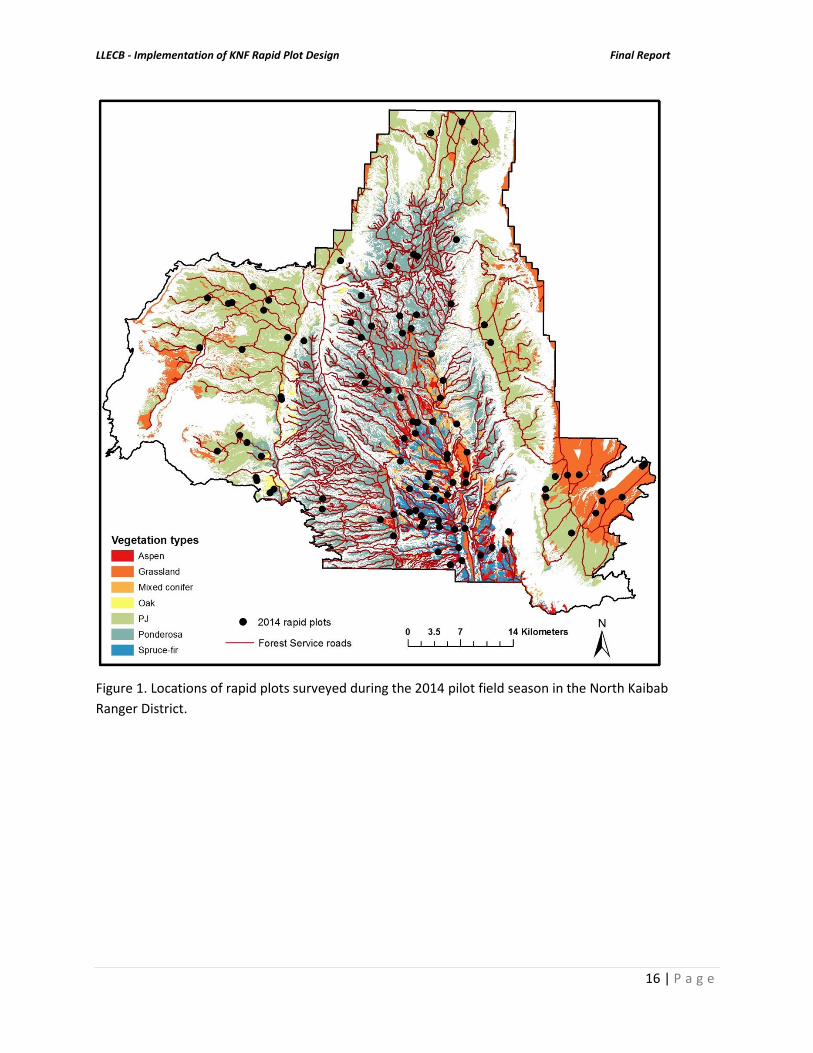
Figure 1. Locations of rapid plots surveyed during the 2014 pilot field season in the North Kaibab

Ranger District.


17 | P a g e

Figure 2. Locations of rapid plots surveyed during the 2014 pilot field season in the Williams

and Tusayan Ranger Districts.


18 | P a g e

Figure 3. Relative proportions of the different invasive species detected in rapid plots across the North Kaibab, Tusayan, and Williams Ranger Districts during the 2014 pilot field season.

Thistle species

Cheatgrass

Russian thistle

Knapweed species

Dalmation toadflax

Other

lab of landscape ecology and conservation biology final

Documents