Lab 8: Faraday Effect and Lenz’ law Phy208 Spring 2008 Name_____________________________ Section___________

This sheet is the lab document your TA will use to score your lab. It is to be turned in at the end of lab. To receive full credit you must use complete sentences and explain your reasoning clearly. What’s this lab about? In this lab you investigate effects arising from magnetic fields that vary in time. There are three parts to the lab: PART A Move a bar magnet through a coil of wire to investigate induced EMF and current. PART B Drop a strong magnet through various copper tubes to investigate the forces caused

by induced current. PART C Quantitatively investigate Faraday’s law by using a time-dependent current through a

coil of wire to generate a time-dependent magnetic field. Why are we doing this? Time-varying magnetic fields are all around us, most commonly in electromagnetic waves. But we most often see effects generated by physically moving permanent- or electro-magnets, or by changing the current through an electromagnet. The EMF, electric currents, and forces generated by these can be quite impressive, even enough to help brake a subway car.

What should I be thinking about before I start this lab? Last week in lab you looked at the properties of static (time-independent) magnetic fields, produced by permanent magnets and by loops of current. These static fields varied throughout space in direction and magnitude, but were the same at all times.

This week you discover some very unusual properties of time-varying magnetic fields. In particular, a time-varying magnetic field produces an electric field. This means that there is more than one way to make an electric field.

You can make an electric field with electric charges, as around a point charge or between charged capacitor plates, but also an electric field accompanies a time-varying magnetic field. Wherever there is a time-varying magnetic field, there is also an electric field. For instance, waving a permanent magnet in the air produces an electric field.

In this case the electric field is said to be induced by the time-varying magnetic field. This induced electric field exerts a force on charged particles, and so work is required to move a charged particle against this field.

Pretty much like the electric fields we’ve worked with before, except that there aren’t any electric charges around producing this electric field.

2

A. Induced fields in a loop of wire A simple way to measure this induced electric field is to put a piece of wire where you want to measure the electric field. At any point in a conductor where there is an electric field, there is also a current, according to

!

r j ="

r E , where

!

r j is the current

density,

!

r E is the electric field, and

!

" is the conductivity.

This means that there can be an electric field in the wire, and a current in the wire, without a battery anywhere. Faraday’s law: Faraday discovered a quantitative relation between the induced electric field and the time-varying magnetic field. He found that the EMF around a closed loop is equal to the negative of the time rate of

change of the magnetic flux through a surface bounded by the loop:

!

" = #d$

dt.

The EMF around a closed loop represents the work/Coulomb required for you to move a positive charge around that closed loop. One other difference between EMF and electric potential difference is that the potential difference between two points depends only on the beginning point and the end point, and not the path between them. The electric potential works great for electric fields and forces generated from charges because those forces are conservative. The work done to move a charged particle from point A to point B against these fields depends only on the location of points A and B. This means that an electric field line like this cannot be generated by fixed electric charges. A1. Give one reason why the electric field line above cannot be generated by fixed

electric charges.

3

But these are exactly the kind of field lines that are generated by Faraday’s mechanism! Your book calls these non-Coulomb electric fields, and the ones that can be generated from static charges it calls Coulomb electric fields. A2. Now you measure the EMF induced in coil of wire by a changing magnetic flux. You

will start by using the 800 turn coil on your lab table. Remember that this induced EMF will cause a current to flow in the wire. So connect the 800 turn coil to the Digital Multimeter (DMM), making sure that the DMM is set to measure current.

The long arrow on the coil indicates that the coil is wound clockwise from the bottom terminal to the top terminal

Connect the top terminal to the red terminal of the DMM for this measurement.

Take the long bar magnet and push it into the hole through the coil from the end with the long arrow, watching the current on the DMM. (this is easiest with the coil laying on its side).There is a line across the width of the bar magnet at its North pole.

Turn the bar magnet around, and do it again. Summarize your results in the table below.

Motion Sign of flux Sign of

change in flux

Sign of induced current

N pole moving into coil

N pole moving out of coil

S pole moving into coil

S pole moving out of coil

A3. Explain how this is consistent or inconsistent with Lenz’ law.

Red

Black

4

A4. Now connect the current sensor (small silver box with “Current Sensor” labeled on the top) to channel A of the Pasco system. (There are only four of these, so you will need to share). Open the Lab8Settings1 file from the course web site and record some data: try pulling the magnet very slowly at constant speed, and then a little more quickly at constant speed.

The current sensor only works below 28 mA. This means that if your peak current reaches 28 mA, the measurement is not correct.

Qualitatively explain why the current rises to a peak then falls again. Use what you know about bar magnet field lines, magnetic flux, and Faraday’s law.

A5. Look at the peak current you obtained in A4 when moving the magnet. What EMF

around the loop does this correspond to? (Hint: you can use your DMM to measure the coil resistane resistance). A6. You can also make a measurement that gives you the EMF directly. Unplug the coil

from the current amplifier, and the current amplifier from the Pasco interface. Plug the coil directly into channel A of the Pasco interface. Click on the LabSettings2 file from the course web site. Take data by pushing the bar magnet into and out of the coil, keeping the speed about the same as in A4. Qualitatively compare to your measurement of A4 and A5.

A7. Do A6 again using the 400 turn coil. How do your measurements compare to the

800 turn coil for the same magnet motion?

5

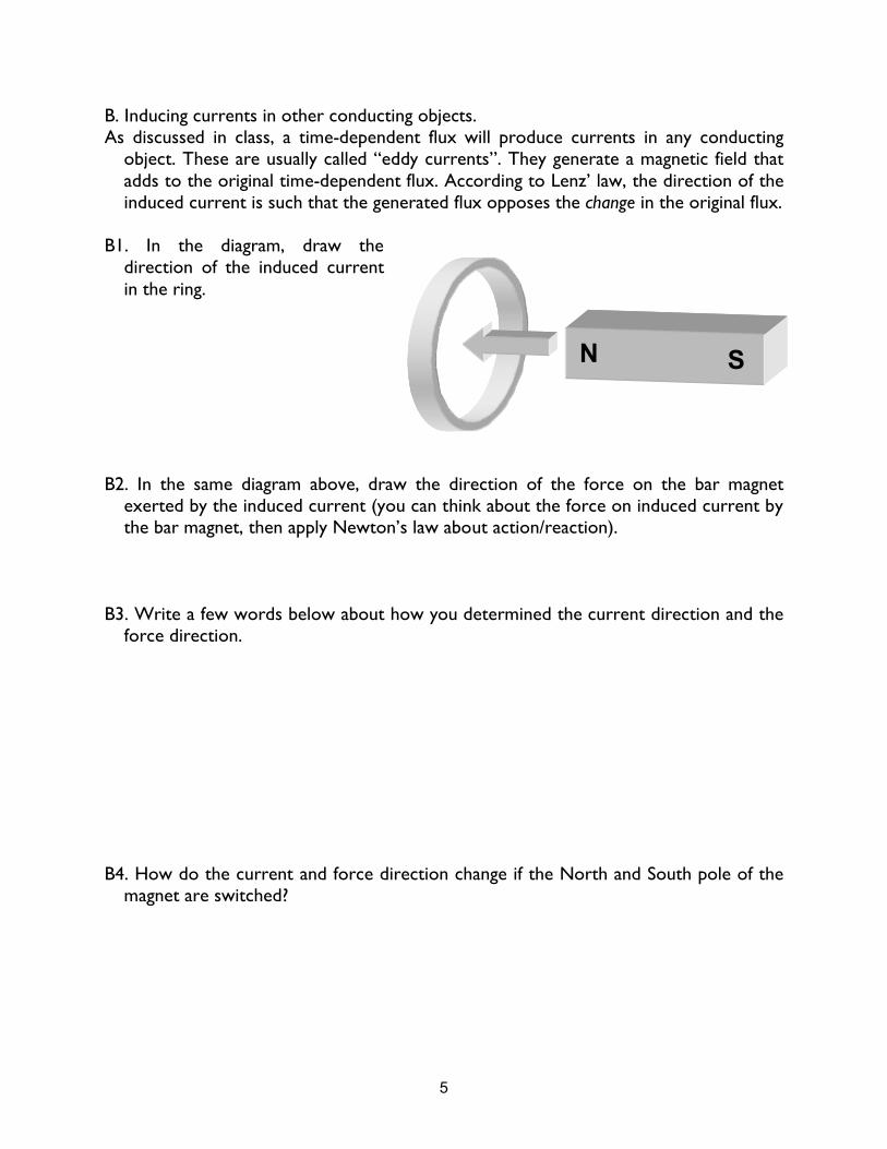
B. Inducing currents in other conducting objects. As discussed in class, a time-dependent flux will produce currents in any conducting

object. These are usually called “eddy currents”. They generate a magnetic field that adds to the original time-dependent flux. According to Lenz’ law, the direction of the induced current is such that the generated flux opposes the change in the original flux.

B1. In the diagram, draw the

direction of the induced current in the ring.

B2. In the same diagram above, draw the direction of the force on the bar magnet

exerted by the induced current (you can think about the force on induced current by the bar magnet, then apply Newton’s law about action/reaction).

B3. Write a few words below about how you determined the current direction and the

force direction. B4. How do the current and force direction change if the North and South pole of the

magnet are switched?

N S

6

B5. You have a 6” length of 1/8” wall copper tube, and a strong NdFeB disc magnet. Hold the tube vertically above the lab table, and drop the disc magnet down the tube. Start the magnet so that the disc surface is parallel to table. Describe below what happened.

B6. The forces on the magnet are the force of gravity, and the force from the currents

induced in the tube, as you investigated in B2 above. Explain why the magnet falls in the tube at a constant speed.

Think of the tube as metal rings (as in B1) stacked on top of each other. B7. Now drop the magnet down the tube so that the flat disc surface is perpendicular

to the lab table. Describe below the motion of the magnet, and explain why it does this. Hint: sketch in the field lines from the magnet.

7

B8. Now you will make a quantitative measurement of how long it takes the magnet to drift down various tubes. Use your stopwatch to time the drift. Do the measurement several times and average, then calculate the terminal velocity.

You will use: [ID = “Inside Diameter”] Two 6” tubes ( 1/8” wall, 1” ID) doubled up lengthwise (you may need to borrow) One 6” length ( 1/4” wall, 1” ID) (there is only one of these) One 6” tube (1/8” wall, 7/8” ID) (everyone should have one of these)

Tube Length Time1 Time2 Time3 AveTime Term. Vel. (cm/s)

1/8 W, 1 ID 30.5cm

1/4 W, 1 ID 15.25cm

1/8 W, 7/8ID 15.25cm

B9. In this section you qualitatively explain the ordering of the terminal velocities (e.g. why the slowest is the slowest and why the fastest is the fastest). Think of the tube as a several rings (as in B1) stacked on top of each other. The induced currents in the tube produce an upward force on the magnet that cancels gravity. The induced currents are determined from the EMF around the ring by the resistance.

i) First think about the two tubes of the same inner diameter (ID) and different wall

thickness. How do the induced currents compare for the same for the same magnet speed?

ii) How does this explain the ranking of the magnet falling speeds in the 1” ID tubes with

1/8 and 1/4 wall thickness?

8

iii) Now think about the two 1/8 wall tubes with different inner diameters. Referring to the picture, how does time rate of change of the flux through a ring depend on the ring diameter (it helps to think about an extremely large ring as a limiting case).

iv) How does this explain the relative falling speeds in the two tubes of 1/8” wall

thickness?

9

C. Quantitative determination of induced fields. Dropping magnets through tubes is a lot of fun, but it is difficult to make quantitative

measurements of induced currents. The magnetic field from a permanent magnet is fairly complicated, and it is difficult to make the flux from it change at a known rate.

In this section you produce a magnetic field by passing a current through a large coil of wire. It takes a lot of current to make any reasonably sized field, so you use a power amplifier controlled by the computer to supply the necessary current to the coil.

The large coil of wire here plays the role of the moving bar magnet of part A. You don’t physically move the large coil, but have the computer make the current through the coil change in time. This produces a magnetic field that varies in time, just as if you were moving a bar magnet.

Just as in part A, you will use this time-dependent magnetic field to induce an EMF in a small coil of wire. This time it is a 2000 turn “sense coil” on a plastic ‘wand’. You will move it around to various locations to make measurements

Before hooking things up, complete the preliminary questions below.

C1. The current in the large coil produces a magnetic field at its center as described by

the Biot-Savart law

!

dB =µo

4"

Idl # ˆ r

r2

. How is this field oriented with respect to the

axis of the coil?

C2. Calculate the cross-product in the Biot-Savart law above, then write an expression for the magnitude of the contribution of a small current element of length dl to the total field at the center of the loop.

C3. Now add up the contributions of each current element along the entire length of the coiled wire of 200 turns to get an expression for the magnetic field at the center of the loop. This is the relation between current through the loop and the magnetic field at the center of the loop.

10

Now you are ready to hook things up.

Connect the power amplifier output to the inputs of one of the large coils. This puts current through the coil. The other large coil is unused.

Use a voltage probe cable to connect Pasco input A to the same large coil as the power amplifier. Input A then measures the voltage drop across the coil through which the power amplifier drives current.

Plug one end of the 8-pin gray cable into the back of the power amplifier and the other end into Pasco input C. Plug in and turn on the power amplifier (switch on back).

Use another voltage probe cable to connect the 2000 turn sense coil to Pasco input B.

Click on the Lab8Settings3 file to start up the data acquisition system. Click start to begin acquiring data.

You should have a real-time display of the voltage drop across the large drive coil (input A), and any induced voltage in the 2000-turn sense coil (input B).

Move the 2000-turn sense coil near the drive coil, watching the induced EMF (input B) on the computer screen. Position the sense coil at the center of the large coil by sliding it onto the metal bar.

C4. Use a 10 Hz triangle-wave for the current in the large coil. Describe the time-dependence of the induced emf in the small coil, and explain the shape of its waveform using Faraday’s law (e.g. why is it not a triangle wave like the drive?)

11

C5. In C4 you saw that the EMF around the sense coil is constant over some period of time. Here you calculate the numerical value of this constant EMF in the sense coil.

i) Calculate the flux through the sense coil for a drive coil current of 1 amp (Assume the magnetic field (C3) is constant over the sense coil area, use the average radius of the sense coil, 1.43 cm, to determine the sense coil area, and use the 10.5cm average radius of the drive coil to determine the field at the drive coil center).

ii) The triangle voltage wave sent to the drive coil by the computer makes the drive-coil current change at a constant rate. For your 10 Hz triangle wave, calculate the time-rate-of-change of the current through the drive coil (drive coil resistance=7Ω).

iii) From i) and ii), calculate the time-rate-of-change of the flux through the sense coil for your 10 Hz triangle wave.

iv) From iii), calculate the EMF around the sense coil and compare to your measurement.

12

C6. Take your bar magnet and wave it around near the drive coil while the data acquisition is running. Explain what is happening.

C7. Take the sense coil off the bar but hold it on the axis of the large drive coil. Slowly change direction of the axis of the coil (e.g. parallel/perpendicular to drive coil axis) and watch the display on the computer. Explain these results.

C8. Change the frequency of the triangle to 20 Hz. Describe and explain how the sense coil EMF has changed from the 10 Hz frequency setting.