1

LAB 7 – Writing Assembly Code

Goals

● Learn to program a processor at low level.

● Implement a program that will be used to test your own MIPS processor.

● Understand the different addressing modes of the processor.

To Do

● In the remaining last three labs, we will build a MIPS processor. In this lab, we will learn how to

program the processor using MIPS assembly language. First, we will write a simple program that

adds all positive integers for a given range (e.g., A + (A+1) + … + B, such that A <= B) using a

subset of the MIPS instruction set.

● We will also implement a more complex program using MIPS assembly language: the Sum of

Absolute Differences (SAD). which is used in various image-processing applications to measure

similarity between parts of images.

● We will test the programs we implement using the MARS simulator. We provide the simulator at:

https://safari.ethz.ch/digitaltechnik/spring2020/lib/exe/fetch.php?media=lab7_files.zip

● For this lab, it is essential to have a thorough understanding of MIPS Programming (Lectures 9

and 10). If you have difficulties, go again through the slides and the lecture videos. You can also

use the MIPS Cheat Sheet that you can find in the course website:

https://safari.ethz.ch/digitaltechnik/spring2020/lib/exe/fetch.php?media=mips_reference_data.pdf

● Follow the instructions. Paragraphs that have a gray background like the current one denote

descriptions that require you to do something.

● To complete the lab, you have to show your work to an assistant before the deadline. The required

tasks are clearly marked with gray background throughout this document.

● You will have an additional exercise in the report.

Introduction

Computer systems are intended to run complex programs. Most application programs are written in a high-

level language, like C, C++, and Java, which are programmer-friendly. However, in order to actually execute

them, they need to be translated into basic operations a processor can execute, that is, assembly language.

Writing assembly code can be tedious, but it allows you to have full control on what is executed: your

processor executes exactly those instructions you specify in the assembly code.

In the following labs, you will build a simple processor with your ALU from Lab 5 as its execution unit.

In this lab, you will write some programs using the basic operations that your ALU from Lab 5 supports. So

far, your ALU only implements a limited set of instructions, but in the next labs you will complete it and you

will be able to actually execute real-world complex programs.

Part 1. A Simple Program That Uses a Limited Set of Instructions

In this exercise, we write an assembly-level program for the MIPS processor that uses the ALU that we built

in Lab 6, which only supports a limited set of arithmetic instructions. The goal of the program is to find the

sum of positive consecutive integers starting from A to B:

S = A + (A+1) + (A+2) + … + (B-1) + B (1)

2

As you may know, this sum can be calculated using the Gauss equation. Unfortunately, Gauss equation

method requires multiplication and division, neither of which can be implemented directly by our current

ALU. However, we will add these instructions in Lab 9. Thus, for now, we cannot use this shorter approach.

One interesting feature about microprocessors is that, although they are fairly limited in what they can do,

they can do it very fast. While adding 1000 numbers might have been a daunting task for the little Gauss

when he was in school, even our comparatively slow processor (running at 50 MHz) can sum up a million

numbers faster than you can blink your eye. This is the main benefit of computer systems: They execute a

very large number of calculations very fast.

If you look at the ALU from Lab 6, you see that only ADD, SUB, SLT, XOR, AND, OR, and NOR

instructions are supported directly by the ALU. Even though we have not implemented J, ADDI, or BEQ

instructions yet, feel free to use them all if necessary.

Refer to Lecture 9 and 10, and the MIPS Cheat Sheet, to learn about these instructions or use instruction

description within the MARS simulator (more on this further down).

Details

One problem with our program is the communication with the rest of the World. Both inputs A and B are 32-

bit numbers and the result S is also 32-bit wide. We learn about input/output (I/O) in the next exercise (2.).

The first thing to do is loading the inputs A and B into registers. If you inspect your instruction set, you will

notice that there is only one convenient way of tackling this problem – the ADDI instruction. Thus, you will

start by initializing the registers with inputs A and B. The ADDI approach (look up details about the ADDI

instruction) only handles 16-bit signed numbers, which means that your inputs A and B must be 16-bit

numbers. This is enough to solve the problem at hand. Once we learn more about I/O, we will be able to load

32-bit values directly from memory using the LW instruction.

When you calculate the sum at the end of your program, store the sum into register $t2. When we learn more

about the SW instruction (and implement it in our own processor), we will be able to store our result into

memory.

When writing your program, you can use temporary registers $t0 to $t7 to hold your variables.

You will use MARS simulator to write an assembly program for performing the computation in Equation (1).

In this part, you are allowed to use only the instructions our ALU supports and J, ADDI, and BEQ.

Using the Java-based MARS simulator

To see whether or not the program works correctly, we use a simulator called MARS, that is able to simulate

the (real) MIPS instruction set. Please note that the program will accept all MIPS instructions, even those we

have not implemented yet, so you have to make sure that you only use instructions from the following subset:

ADD, SUB, SLT, XOR, AND, OR, NOR, J, ADDI, BEQ

Now, let us start the MARS simulator by running the provided run_mars.bat script. If the program does not

start correctly, please make sure that your folder is located on a local disk, and not on a network drive, as this

may cause some problems.

3

Figure 1. MARS main

Click the Open button and select the lab7.asm file, which we provide for this lab. The file contains a basic

code skeleton for you to use.

Next, go to Settings → Memory Configuration as shown in Figure 2. Once there, select “Compact, Data at

Address 0” option and save.

Figure 2. MARS settings

4

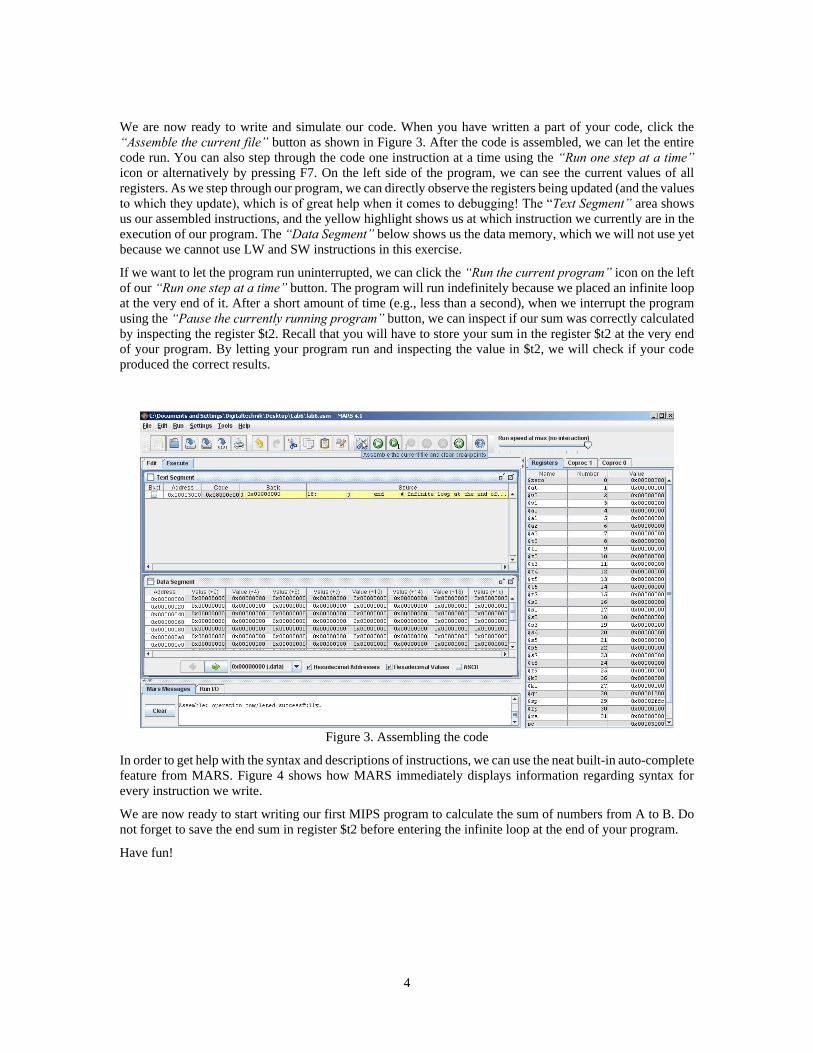
We are now ready to write and simulate our code. When you have written a part of your code, click the

“Assemble the current file” button as shown in Figure 3. After the code is assembled, we can let the entire

code run. You can also step through the code one instruction at a time using the “Run one step at a time”

icon or alternatively by pressing F7. On the left side of the program, we can see the current values of all

registers. As we step through our program, we can directly observe the registers being updated (and the values

to which they update), which is of great help when it comes to debugging! The “Text Segment” area shows

us our assembled instructions, and the yellow highlight shows us at which instruction we currently are in the

execution of our program. The “Data Segment” below shows us the data memory, which we will not use yet

because we cannot use LW and SW instructions in this exercise.

If we want to let the program run uninterrupted, we can click the “Run the current program” icon on the left

of our “Run one step at a time” button. The program will run indefinitely because we placed an infinite loop

at the very end of it. After a short amount of time (e.g., less than a second), when we interrupt the program

using the “Pause the currently running program” button, we can inspect if our sum was correctly calculated

by inspecting the register $t2. Recall that you will have to store your sum in the register $t2 at the very end

of your program. By letting your program run and inspecting the value in $t2, we will check if your code

produced the correct results.

Figure 3. Assembling the code

In order to get help with the syntax and descriptions of instructions, we can use the neat built-in auto-complete

feature from MARS. Figure 4 shows how MARS immediately displays information regarding syntax for

every instruction we write.

We are now ready to start writing our first MIPS program to calculate the sum of numbers from A to B. Do

not forget to save the end sum in register $t2 before entering the infinite loop at the end of your program.

Have fun!

5

Figure 4. Code autocomplete feature of MARS

Use the MARS simulator to write an assembly program that calculates the sum in Equation (1). Use only the

instructions ADD, SUB, SLT, XOR, AND, OR, NOR, J, ADDI and BEQ. Initialize your data (A and B)

using the ADDI instruction, and store your result in $t2.

Part 2. A More Complex Program - Sum of Absolute Differences (SAD)

Sum of absolute differences (SAD) is a widely-used algorithm for measuring the similarity between images.

It works by calculating the absolute difference between each pixel in the original image and the corresponding

pixel in the image being used for comparison. These differences are summed to create a simple metric of

image similarity.

For example, see the following images:

Figure 5. Images to calculate the Sum of Differences

They look the same, right? Well, that is not true. Although it cannot easily be appreciated, they have been

taken from slightly different camera angles, so that the right image is shifted with respect to the left image.

The sum of absolute differences provides the following disparity map:

6

Figure 6. SAD disparity map

The sum of absolute differences may be used for a variety of purposes, such as object recognition, generation

of disparity maps for stereo images, and motion estimation for video compression.

In this exercise, you will implement the SAD algorithm. In the previous exercise, we were not allowed to use

the entire MIPS instruction set, although the MARS simulator actually implements all MIPS instructions. In

this exercise, you are allowed to use the entire MIPS instruction set.

The C code of the SAD algorithm is:

// Implementation of the absolute value of differences int abs_diff(int pixel_left, int pixel_right) {

int abs_diff = abs(pixel_left - pixel_right); return abs_diff;

} // Recursive sum of a vector int recursive_sum(int arr[], int size) { if(size == 0) return 0; else return recursive_sum(arr, size-1) + arr[size-1]; } // main function int main() { int sad_array[9];

int image_size = 9; // 3x3 image // These vectors must be stored in memory int left_image[9] = {5, 16, 7, 1, 1, 13, 2, 8, 10}; int right_image [9] = {4, 15, 8, 0, 2, 12, 3, 7, 11};

for (i = 0; i < image_size; i++)

sad_array[i] = abs_diff(left_image[i], right_image[i]);

sad_value = recursive_sum(sad_array, image_size); }

For those of you who like to do a more ambitious task, we are happy to provide you one.

If you breezed through the exercise until now, and want a tougher nut to crack, here is your chance. In

many of the tasks below, you will have two options: either implement the code by yourself or use the code

we provide. In any case, choose the one that suits your challenge needs.

7

You don’t get extra points if you choose the challenging option, but any of this could actually be

asked in the exam, so it is a good idea if you try it ☺.

Open in MARS the file lab7_sad.asm. It contains the necessary part of the code to implement the SAD

algorithm. Pay attention to the comments: “TODO”, since you will have to complete the code according to

the instructions in the following subsections.

2.1. Initializing data in memory

Images are stored in the data memory as an array of pixels. Each pixel in the image is represented by a value

from 0 to 16 that represents the grayscale. For example, an image of 3x3 pixels is stored as an array of 9

elements (e.g., left_image[]), and each element of the array corresponds to a pixel in the image as follows:

left_image[0] left_image[1] left_image[2]

left_image[3] left_image[4] left_image[5]

left_image[6] left_image[7] left_image[8]

In the previous exercise, we could not use the LW and SW instructions, and we had to initialize the data by

storing it directly in the registers. That worked because we had little data, but in general, a program works

with large amounts of data and it must be stored in memory. In this exercise, we store the image pixels in

memory.

Make sure that the data segment in your memory starts at address 0x00000000 (see Figure 7). The layout

of your memory should look like the following:

Figure 7. Memory layout

Complete the section in the code “Initializing data in memory” using the SW instruction and the initial data

specified in the C program (TODO1)

8

2.2. Implement the abs_diff() routine

The abs_diff() function takes two arguments (one pixel for the left image, and one pixel for the right

image), and returns the absolute value of their difference. Check Lectures 9 and 10, and Chapter 6 in “Harris

& Harris”, to remember how to access the arguments within the routine, and where to store the return value.

Although there exists a pseudo-instruction that calculates the absolute value (abs), you are not allowed to

use pseudo-instructions. You have to implement code which calculates the absolute value by yourself.

Option 1 (challenging): Write assembly code for the routine abs_diff(int pixel_left, int pixel_right) (TODO2)

Option 2 (easy): Download the helper_abs_diff.asm file from the course website and copy the code of this

function into Lab7_sad.asm file (TODO2)

2.3. Implement the recursive_sum() routine

The recursive_sum() function takes two arguments: the base address of a vector, and its size. It returns

the sum of all the vector elements.

Option 1 (challenging): Write in assembly the recursive function recursive_sum(int arr[], int size). It takes as first argument the address of the first element of the array sad_array[], and the second

argument is the number of pixels in the image. Note that this is a recursive function and therefore needs to

store the corresponding registers on the stack before calling the recursive function, because otherwise they

are overwritten by the function called (TODO3)

Option 2 (easy): Download the helper_recursive_sum.asm file from the course website and copy the code

of this function into lab7_sad.asm file (TODO3)

2.4. Complete the main function to do the corresponding function calls

As you can see in the C code, in the main function we have to loop over the elements of the images, and then

call the abs_diff() routine.

Under the TODO4, fill in the section “loop:” to loop over the elements of the image. To get the image pixels,

you will have to use the LW instruction. Then, call the routine abs_diff() for every pair of pixels.

Remember to put the arguments in the corresponding registers. After executing abs_diff(), store the result

in the corresponding position of sad_array[]. After the execution of the loop, jump to end_loop. You will

implement that part of the code later.

After the execution of the loop, add all the elements of the array sad_array[] using the recursive_sum()

function implemented before, and store the final result in $t2.

Under the TODO5, complete the section “end_loop”: to prepare the arguments for the function call to

recursive_sum(), and store the result in $t2

Once you have implemented the code, follow the same steps as in the previous exercise, to test your program.

You can check the contents of the memory. At the end of the simulation, your memory and register $t2 should

look like follows:

9

Figure 8. Memory contents after running the program

Last Words

In this exercise, we were given a problem description for a computer system. Since we knew the capabilities

of the ALU of our processor at this point, we were able to select the correct instructions and translate our

idea into a series of instructions for the MIPS processor that calculated the desired result. This is essentially

what a compiler does.

It is clear that we would have been able to calculate the result for the first exercise much faster if we had

implemented multiplication and/or arithmetic shift operations. We will return to this point in Lab 9.

The basic idea behind complex digital systems is that if you are able to perform a lot of simple calculations,

you can make very complex operations. Take video processing as an example. A modern high definition

picture consists of 1920 x 1080 picture elements (pixel), which roughly equals to 2 million pixels. For video,

at least 25 of such pictures must be created each second. This means that if we want to manipulate a high

definition video we need around 50 million operations per second. Assuming that the operation is simple

(e.g., creating a negative image) even the MIPS processor that we are currently building on the FPGA board

is able to perform that.

Memory contents Final result in $t2