MNRAS 000, 1–12 (2018) Preprint 23 April 2018 Compiled using MNRAS LATEX style file v3.0

Precision stellar radial velocity measurements withFIDEOS at the ESO 1-m telescope of La Silla

L. Vanzi1,2?, A. Zapata1,2, M. Flores1,2, R. Brahm3,1, M. Tala Pinto4,1, S. Rukdee1,2,

M. Jones5, S. Ropert1,6, T. Shen1, S. Ramirez1, V. Suc1,6, A. Jordan7,3,8, N. Espinoza8,3,7.1Centre of Astro-Engineering, Pontificia Universidad Catolica de Chile, Av. Vicuna Mackenna 4860, Santiago Chile2Department of Electrical Engineering, Pontificia Universidad Catolica de Chile, Av. Vicuna Mackenna 4860, Santiago Chile3Millennium Institute of Astrophysics, Santiago, Chile4Landessternwarte, Zentrum fur Astronomie der Universitat Heidelberg, Konigstuhl 12, D-69117, Germany5European Southern Observatory, Alonso de Cordova 3107, Casilla 19001, Santiago, Chile6Obstech SpA, Nueva Providencia 1881, of. 1620, Santiago Chile7Institute of Astrophysics, Pontificia Universidad Catolica de Chile, Av. Vicuna Mackenna 4860, Santiago Chile8Max-Planck-Institut fur Astronomie, Konigstuhl 17, Heidelberg D-69117, Germany.

Accepted April 10, 2018. Received January 17, 2018

ABSTRACTWe present results from the commissioning and early science programs of FIDEOS, thenew high-resolution echelle spectrograph developed at the Centre of Astro Engineeringof Pontificia Universidad Catolica de Chile, and recently installed at the ESO 1mtelescope of La Silla. The instrument provides spectral resolution R ∼ 43,000 in thevisible spectral range 420-800 nm, reaching a limiting magnitude of 11 in V band.Precision in the measurement of radial velocity is guaranteed by light feeding withan octagonal optical fibre, suitable mechanical isolation, thermal stabilisation, andsimultaneous wavelength calibration. Currently the instrument reaches radial velocitystability of ∼ 8 m/s over several consecutive nights of observation.

Key words: Spectrographs – Radial Velocities – Spectroscopic – Planetary Systems

1 INTRODUCTION

High resolution spectroscopy is an extremely valuable toolin the study of a wide variety of celestial objects and phe-nomena. Observations of great interest can be obtained withthis technique almost with any size telescope. In particularmoderate size telescopes proved to be an extremely usefulcomplement to bigger instruments when equipped with suit-able spectrographs. It is mainly for this reason that our teamembraced the challenge of providing the scientific commu-nity with spectrographs able to make the best use of thesmall and medium size telescopes available in Chile, whichcurrently tend to be underused or decommissioned. At thesame time, through this work we aim at building up an expe-rience in astronomical instrumentation that was not presenthitherto in the Chilean community. Our first effort in this di-rection was the spectrograph PUCHEROS installed at theUC Observatory Santa Martina (Vanzi et al. 2012). Thisproject proved to be a success, as it has been in operationduring the last seven years, proving to be a precious toolfor teaching experimental astronomy, at the undergraduate

? E-mail: lvanzi@ing.puc.cl

and graduated level, and also for producing scientific results,which are of surprising significance and quality when com-pared to the modest aperture of the telescope and to thefar-from-optimal location of the observatory (e.g. Coronadoet al. 2015; Izzo et al. 2015; Bluhm et al. 2016; Arcos et al.2017). This positive experience motivates our team, at theCentre of Astro Engineering UC (AIUC), to continue withenergy this line of work. In particular the measurement ofhigh precision radial velocity (RV) is a field where relativelysmall aperture telescopes can provide outstanding resultscontributing significantly to a number of research fields inastrophysics as the study of binary and multiple stellar sys-tems, astro-seismology, and the search for exoplantes. It isfor these reasons that we concentrated our efforts in over-coming the limitation of PUCHEROS, mainly the quality ofthe site (located at about 22 km from the centre of Santi-ago), the small aperture of the telescope (50 cm), the lowefficiency of the detector (∼ 60%), and the modest stabil-ity for RV measurements (typically 50-100 m/s). All thiswas casted into a new instrument called FIbre Dual EchelleOptical Spectrograph or FIDEOS, which recently saw firstlight at the ESO 1m telescope of La Silla. The main scientificdriver of the instrument is to provide spectroscopic follow-

c© 2018 The Authors

arX

iv:1

804.

0744

1v1

[as

tro-

ph.I

M]

20

Apr

201

8

2 L. Vanzi et al.

up for photometric transit surveys searching for exoplanetsaround bright stars such as TESS (Ricker et al. 2014), MAS-CARA (Talens et al. 2017), or the upcoming HATPI1. Toachieve this purpose, FIDEOS aims at reaching a limitingmagnitude V=11 and a RV precision better than 10 m/s, al-lowing a comfortable detection of the reflex motion inducedon nearby stars by gas giant planets. One of the challengesof the project was to reach these performances within thestrong constraints of the budget available for the hardware(< 100 K EUR). In this paper we present: a general de-scription of the system in Section 2 including instrumentand telescope; results from the commissioning in Section 3;results from early science programs in Section 4; and con-clusions in Section 5.

2 INSTRUMENT AND TELESCOPE

In this section we present the general instrument concept,details of the opto-mechanical design and the general systemsetup. We also describe the refurbishment of the ESO 1mtelescope control that was implemented by our team. Theinstrument includes three main parts, the spectrograph, thecalibration unit, and the telescope interface. They are con-nected one with another by optical fibres. To limit the cost,moderate price off-the-shelf components were selected when-ever possible or were manufactured in house. A preliminarydesign of FIDEOS was presented by Tala et al. (2014), how-ever there have been significant modifications since, whichmake it worth updating the instrument description here.

2.1 Spectrograph

The spectrograph uses a classic echelle configuration, the op-tical components are as follows. The collimator is a parabolicmirror of 762 mm focal length, 152.4 mm in diameter byEdmund Optics with enhanced aluminium coating and itis used off-axis . The echelle is R2.75, with 44.41 gr/mm,110×60 mm in size by Richardson gratings, it is mountedwith an off axis angle γ ≈ 4◦. Cross dispersion is provided bytwo identical prisms of SF11 glass with apex angle of 34.6◦

manufactured by Pecchioli Research and mounted with anangle of 64.4◦ between one an other. Finally the objective is acommercial Canon-EF-300 mm f/4 photographic objective.

The spectrograph is illuminated by two 50 µm core low-OH fibres through a tele-centric re-imaging system, whichprovides a magnification 4. The two fibre cross sections areoctagonal to improve the scrambling effect (Chazelas et al.2010; Avila 2012), they are separated by 110 µm center-to-center and they are mounted in a single FC connector. Thefibre cable was provided by Ceramoptec. One fibre bringsthe light from the telescope to the spectrograph (science fi-bre), the other carries the light from the calibration unit forsimultaneous wavelength reference (calibration fiber). Thetelecentric system is assembled on a 30 mm ThorLabs cagestage and it includes two achromatic doublets of 7.5 and 30mm focal length respectively, separated by the sum of theirfocal lengths, the beam from the fibre is received at f/5 andilluminates the collimator at f/20. The slow beam allows to

1 http://hatpi.org

Figure 1. Top view of the opto-mechanical layout of the spec-

trograph, the optical components are identified by labels.

obtain excellent image quality with the commercial collima-tor. Because the images of the fibres have a diameter of 200µm the theoretical spectral resolution of the spectrographis about 21000, which is boosted by a factor 2 with a 2ximage slicer. Details of the slicers are presented in Tala etal. (2017). The collimated beam is 38 mm in diameter.

The collimator and the echelle are mounted on kine-matic mounts designed and manufactured at the AIUC, bothsupports allow tilt around two axis with micro-metric screwsfor precise alignment. The prism and objective are mountedon static mounts. The whole setup is arranged on a Thor-Labs aluminium bread board of 900×600 mm and protectedby an enclosure.

As detector we employ a PL-230 Finger Lake Instru-ments (FLI) camera, which includes a back illuminated Mid-band e2v CCD 2K×2K with pixel size of 15 µm. The cameracomes with a convenient USB connection. Because the op-tics of the spectrograph has a reduction factor of 2.5, the100 µm size half-fibre is imaged on 40 µm providing a spec-tral sampling of 2.6 pixels. The FLI camera is mounted on acarbon-fibre support that guarantee stiffness and minimisethe heat transfer to the optical bench and optics. This sup-port, that was also designed and manufactured at the AIUC,allows rotation around an axis perpendicular to the opticalbench and shift in the direction of the optical axis for fo-cusing. The CCD is operated at a temperature of -35 C andread out speed of 500 kHz, in these conditions we measureda read out noise of 11 e− and a negligible dark signal, bothvalues within the specifications of the manufacturer. Theoperation temperature is reached and maintained by ther-moelectric cooling, the dissipated power is about 45 W andit is removed via a recirculating liquid chiller. To this effectwe use a liquid chiller CW-5000 by S&A. The chiller main-tain the enclosure of the FLI camera at a temperature of 19C with a stability of about 0.1 C peak-to-peak.

The top view opto-mechanical layout of the instrument,with the optical elements identified, is shown in Fig. 1, animage of the spectrograph assembly is showed in Fig. 2.

2.2 Calibration Unit

The calibration unit includes a ThAr lamp for wavelengthcalibration and a continuum halogen lamp for order def-

MNRAS 000, 1–12 (2018)

FIDEOS at the ESO 1m telescope 3

Figure 2. FIDEOS spectrograph and enclosure. In the front of

the image on the left side the optical fibre with the feeding telecentric optics and the echelle are visible. To the right the collima-

tor parabola. In the centre the two cross dispersing prisms and

the objective. In the back the CCD camera.

inition and flat fielding. The ThAr lamp is provided byPhotron, the halogen lamp is a HL2000-FHSA of Ocean Op-tics. To improve the red to blue balance of the continuum weuse a daylight blue filter LB-120 of Edmund Optics. Bothlamps are imaged through the same optics on two fibresmounted on the same connector. This configuration forcesto have both fibres illuminated at the same time with eitherlamp. One fibre goes to the spectrograph providing simul-taneous wavelength reference (calibration-fibre), the othergoes to the telescope interface and can illuminate the sciencefibre (illumination-fibre). A beam splitter is used to mergethe two optical beams with a balance 90% ThAr, 10% halo-gen. The two lamps are never ON at the same time. Theintensity of the ThAr lamp can be adjusted positioning aneutral density filter which is mounted on a linear stage.

2.3 Telescope Interface

The telescope interface connects the science-fibre with thetelescope making possible its illumination by the astronom-ical source. The light from the source enters the systemtrough a pinhole of 125 µm diameter, equivalent to 1.9 arc-sec on the sky. The pinhole is drilled in a reflective surfacewhich allow to re-image the field around the target on anacquisition camera to perform centring and guiding. Theacquisition camera is an Imaging Source DMK33UP13001280×1024 pix and pixels of 4.8 µm. The acquisition optics isa split triplet (Smith 2004), it employs a BK7 custom madelens and two commercial doublets - Thorlabs AC508-100-Aand AC300-050-A. The lay out of the acquisition optics isshown in Fig. 3. The effective focal length of the system is81.3 mm and the focal working ratio is F/4.1. The field ofview is 4.4×3.5 arcmin with a scale of about 0.21 arcs/pix.The pinhole is re-imaged on the head of the science-fibre byan achromatic triplet of 12.5 mm focal length, 6.5 mm di-ameter by Edmund Optics. The science-fibre feeding systemis mounted in a 30 mm ThorLabs cage, the science-fibre

Figure 3. Detail of the acquisition optics with two folding mirrors

and a split triplet. The first folding mirror has a pinhole in its

centre which is the entrance of light to illuminate the sciencefibre.

was initially supported by a five axis mount, however thetilt adjustment proved to be unnecessary and the stage wassubstituted with a simpler XY mount which also guaranteesbetter stability against flexures and temperature variations.

The telescope interface includes a tip-tilt correction sys-tem for optimal light feeding. This function is provided bya commercial Starlight Express AO system, the control wasdeveloped by us. The centroid of the target (weighted bylight intensity) is calculated from the images of the acqui-sition camera, the error in pixels is translated to an errorin distance at the focal plane and the steps needed for thecorrection are calculated. The correction is applied tilting aplane parallel plate controlled in two axis by step motors.The system is controlled at a speed up to 10 Hz proving veryeffective for fast tracking errors and to some extent for at-mospheric tip-tilt correction. The improvement in efficiencycan reach up to 50% in poor seeing conditions.

The telescope interface also receives the illumination-fibre from the calibration unit allowing injection of the cali-bration light into the science-fibre. This is done with a mov-ing prism that can be inserted between the pinhole and thefibre-feeding-optics with a linear motorised stage. Becausethe calibration-fibre and the illumination-fibre are always il-luminated at the same time, a shutter covers the end of theillumination-fibre during the observations to avoid light con-tamination in the telescope interface. A sketch of the systemis shown in Fig. 4.

The telescope interface also allows to redirect the beamof the telescope with a folding mirror toward a lateral auxil-iary port that can receive a guest camera. The interface itselfis an aluminium structure measuring 500×250×250 mm andweighting 32 Kg.

MNRAS 000, 1–12 (2018)

4 L. Vanzi et al.

Figure 4. Detail of the fibre feeding system at the telescopeinterface. The beam from the telescope comes from the top of the

image and reaches the science-fibre through the pinhole and theachromatic triplet. A prism can be inserted in the path (moving

perpendicular to the plane of the image) to redirect the light

from the illumination-fibre, on the left side of the image, to thescience-fibre. When the prism is not inserted a shutter covers the

illumination-fibre.

2.4 Instrument control and data acquisition

There are a number of functions in the instrument that re-quire suitable control, mainly the two calibration lamps andthe neutral density filter in the calibration unit, the calibra-tion prism in the telescope interface. There are no movingparts in the spectrograph. The neutral density filter and thecalibration prism are both mounted on linear stages that re-fer to a home position defined by a mechanical limit switch.The low level control of the calibration module is providedby an Arduino Mega, working with an Ethernet shield whichprovides remote access. The calibration lamps are controlledthrough a relay board designed and built at AIUC. The Neu-tral Density filter linear stage is operated by a stepper motorcontrolled through a motor driver board based on the H-bridge driver Chip L298N. The Arduino hosts a web basedengineering GUI which provides a control interface for thedifferent devices. Integration with the spectrograph’s maincontrol system is given by HTTP methods and the informa-tion is formatted in JSON.

We implemented a classical instrument control softwarearchitecture, which comprises an observation control subsys-tem (OCS), an instrument control subsystem (ICS), and adetector control system (DCS). The OCS is the orchestra-tor of the observation, which interfaces the telescope (TCS)to acquire a target, configure the hardware devices throughthe ICS and take an exposure by commanding the DCS.These processes were implemented on top of the InternetCommunication Engine (ICE), a distributed programmingframework 2. The scientific CCD is controlled by the DCSprocess through the USB connection. The DCS controls theexposure time, shutter, and temperature control loop. Theacquisition camera is controlled by a second TCS process,which runs inside of an Odroid system, and continuouslycapture snapshots of the field. The image-processing algo-

2 https://zeroc.com/products/ice

rithm is implemented on top of OpenCV 3. The OCS hidesthe complexity of the other subsystems and exposes high-level information to the operators through a web browser.Several dashboards were created in order to monitor the sta-tus of each subsystem during operation. A GUI was createdto allow interactive observation, but at the same time, abatch mode could execute a list of calibrations in an unat-tended manner.

2.5 Data processing

The data processing is performed by a dedicated pipeline de-veloped within the CERES framework (Brahm et al. 2017).The pipeline has basically the same structure of the CERESpipelines developed for other similar instruments (Coralie,FEROS, FIES). The steps automatically performed are: ini-tial classification of the images according the data type (bias,flat, ThAr lamp, science image), standard image reductionroutines, identification and tracing of the echelle orders forthe science and comparison fibres, optimal extraction (Mar-shal 1989) of the science frames and ThAr calibration im-ages, determination of the wavelength solution for the ThArcalibration and simultaneous calibration spectra, determi-nation of the instrumental drift in wavelength, using the si-multaneous wavelength calibration mode, correction of theblaze function and continuum normalisation of the extractedscience spectra. The pipeline also provides barycentric cor-rection, measurement of the RV using the cross-correlationtechnique, measurement of the bisector span of the cross-correlation peak, quick determination of the stelar atmo-spheric parameters (Te f f , log(g), and [Fe/H]) and vsini ofthe science spectra.

One particular adaptation of the pipeline for this newinstrument is related to the treatment of the wavelength cal-ibration of the ThAr spectra from the calibration fiber. Theprofile of an extracted narrow emission line is, at first order,symmetric in the case of the science fibre.This is because theimages produced by the two slices of the fibre are aligned inthe cross-dispersion direction (Tala et al. 2017). This sym-metry allows to model the line profile with a simple gaussianfunction, where the mean is adopted as the position of theemission line which is then used to compute the wavelengthsolution. For the calibration spectrum instead only half fibreis used and this produces asymmetric lines in the extractedspectrum.The asymmetry gets partially blurred out by theinstrumental profile, but nonetheless, modelling these lineswith a gaussian can introduce systematic effects due to ”pix-elization”. For this reason we use the analytic expression ofa collapsed half circumference of known diameter, convolvedwith a normalised gaussian that represents the instrumentalprofile. The free parameters of this model are the centralpixel position, the intensity of the half circumference, andthe width of the gaussian.

The pipeline generates two output spectra for each sci-ence frame. One contains the full wavelength coverage ofthe instrument considering the 50 echelle orders, while thesecond output spectrum contains only the data of the last39 orders, where the 11 reddest orders are not consideredbecause of significant contamination from saturated ThAr

3 http://opencv.org/

MNRAS 000, 1–12 (2018)

FIDEOS at the ESO 1m telescope 5

Figure 5. Representation of the global wavelength solution of

FIDEOS for the different echelle orders (black line). The redpoints correspond to the positions of the 690 emission lines of

the ThAr lamp used to compute the wavelength solution.

lines. For computing the wavelength solution we use ∼ 690ThAr emission lines, typically only a small fraction of them(no more than 20) are automatically rejected from the fitwhen their positions are considered as outlier. The rejectionof this small fraction of lines does not introduce systematiceffects detectable at the level of best precision that we canreach. The typical root mean square of the residuals of thefinal wavelength solution is of ∼ 100 m s−1 which sets thelower limit of the precision that FIDEOS can achieve in RVto 4.0 m s−1 (see Fig. 5, and 6).

2.6 Instrument setup

The setup of the instrument is arranged to optimise sta-bility and efficiency. The spectrograph and calibration unitare conveniently installed in a thermally isolated room at thefirst floor of the telescope building (FIDEOS room). This lo-cation, one floor above ground, one floor below the telescopelevel, is particularly favourable for maintaining a good ther-mal control of the spectrograph. The building walls are thickand provide by themselves some level of isolation this wasfurther improved by covering the walls of the FIDEOS roomwith polystyrene panels. The only sources of heat present inthe FIDEOS room are the scientific CCD, the calibrationlamps and the neutral density filter motor of the calibra-tion unit. The room has no windows and can only be ac-cessed through a larger room (FIDEOS Service room), whichis maintained at 16 C with a regular air conditioning sys-tem. The power supply of the scientific CCD, power supplyof the calibration unit, acquisition and operation computerand the chiller are all located in the service room. The CCDchiller is operated at 14 C. The spectrograph is protectedby a ThorLab black cardboard enclosure which is containedin a larger polystyrene box for optimal thermal isolation.

Therefore there are two layers of thermal isolation. The op-tical breadboard sits on top of an aluminium plate whichis actively stabilised in temperature by a Belektronig HATcontrol model M-20.

To achieve optimal throughput, a critical part of theinstrumental setup is the alignment of the science-fibre atthe telescope interface. To this purpose we proceed in twosteps: i) we back illuminate the science fiber and observe itsimage through the pinhole with a microscope to optimisethe centring, ii) we project a laser beam from the sciencefibre toward the M2 to optimise the tilt angles.

The cable length between the FIDEOS room and thetelescope interface is about 30 m. As explained, we havethree optical fibres, the science-fibre running from the tele-scope interface to the spectrograph (30 m), the calibration-fibre running from the calibration unit to the spectrograph(5m), and the illumination-fibre running from the calibra-tion unit to the telescope interface (30 m) with the purposeof illuminating the science fibre.

2.7 ESO 1m telescope

The ESO 1m telescope is the first telescope that was in-stalled by ESO at the observatory La Silla back in 1966. Itis a classic Cassegrain design with 1 meter clear aperture, fo-cal ratio 13.6, and it provides a scale of 15 arcsec/mm. It wasused as photometric telescope until 1994, later employed inthe DENIS survey from 1996 to 2001 (Epchtein et al. 1997)and then decommissioned. Starting in 2013 the telescope isbeing operated by Universidad Catolica del Norte (UCN).As part of our work to equip the telescope with a new spec-trograph we also installed a completely new control systemwhich provides stable and reliable operation.

The original Telescope Control System (TCS) was run-ning in an HP1000 computer which was obsolete and didnot allow proper remote access and control. The new TCSis conformed by a modern and robust software running ona group of single board computers interacting together asa network with the CoolObs TCS developed by ObsTech(Ropert et al. 2016). The original motors were maintainedand the only mechanical modifications performed were theupgrade of the existing motor encoders and the installationof new on-axis encoders on both RA and DEC. The new TCSallows to combine the input signals of 2 encoders per axis,the telescope axis encoder and the motor encoder, using aExtended Kalman Filter (Kalman 2016; Kalman & Bouchy1961). This configuration achieves a precision of 0.25 arc-second on sky during tracking with moderate cost encoders.

The initial pointing model, embedded in the CoolObsTCS, was obtained with a set of 15 known stars uniformlyspread in the sky. This resulted in pointing residuals be-low 4.5 arc-seconds RMS, which allows us to point the starwithin the guiding camera field of view and very close to thefibre. Automatic re-centring of star on the fibre can then beperformed by the guiding software.

3 COMMISSIONING AND PERFORMANCES

FIDEOS was installed at the telescope and had first lightin June 2016. In this section we report on the main perfor-

MNRAS 000, 1–12 (2018)

6 L. Vanzi et al.

4500 5000 5500 6000 6500 7000Wavelength [A]

−0.008

−0.006

−0.004

−0.002

0.000

0.002

0.004

0.006

0.008

Res

idua

ls[A

]

Figure 6. Residuals in of the wavelength solution. Each point corresponds to the difference between the reference wavelength position

of a particular ThAr line and the value given by the wavelength solution. Different orders are shown with different colours. There is nostructure left in the residuals and the typical rms is of 100 ms−1.

mances of the instrument, in particular the spectral resolu-tion, throughput and stability.

3.1 Spectral resolution and throughput

The spectral resolution was measured from ThAr spectraobserved through the science- and calibration-fibre and mea-suring the FWHM for all emission lines detected, the resultsare shown in Fig. 7.

During the commissioning we measured a number ofspectro-photometric standard stars with different magni-tudes from the catalog of Hamuy et al. (1992, 1994). Theresults are highly dependent on the atmospheric conditionsand, when the sky is clear, on the seeing. The best efficiencyof the whole system turned to be approximately 8% at 550nm. Comparing this number with expectation is not trivialbecause of the large uncertainties on the efficiency of someof the components. The telescope M1 mirror gave 89% whenrecently aluminised, so that we assumed an average value of75% for the efficiency of the telescope. The fibre link hasroughly an efficiency of 60% which is primarily driven byfocal ratio degradation and, at a lower level, by absorptionthrough the fibre and reflection at the fibre end surfaces. Themaximum efficiency of the whole spectrograph, including thedetector, measured in the Lab, is approximately 20%. Thedependency on the seeing is strong. Because the aperture isalmost 2 arc sec in diameter on the sky, we collect 98% ofthe energy with seeing of 0.8 arcesec, 92% with seeing 1 arcs,82% with 1.2 arc sec. Guiding is also a critical aspect whichis largely improved with the tip-tilt system. These valuesprovide a total efficiency of the system fully consistent withthe value reported above. We also measured that the effi-ciency at Hα is 80% of the peak, at Hβ 70%, while 50% ofthe peak is reached at 455 and 730 nm respectively on theblue and red side of the spectrum.

With a read out noise of 11 e−, the photon noise regimefor a star of magnitude V=11, is achieved under good con-ditions in about 15 minutes of integration time. In Fig. 8 weshow the expected signal-to-noise-ratio (SNR) versus expo-

sure time under average observing conditions for V magni-tude from 6 to 12. The theoretical expectation are comparedwith a few measured points. We assume as typical limitingmagnitude V=11 for which SNR of about 10 can be reachedin 30 minutes of exposure.

3.2 Thermal stability

The stability of the instrument is the most critical aspectwhen aiming at precise RV measurements, for this reason wedevoted a significant amount of effort in reaching the bestpossible results on this front. We have been monitoring care-fully the temperature at four critical points of the system,the air in the FIDEOS service room, the liquid of the recir-culating chiller, the enclosure of the CCD camera, and thespectrograph optical bench. The air conditioning system isset to maintain the FIDEOS service room at a temperatureof 16 C, the fluctuations around this set-point are smallerthat 1 C peak to peak, in fact typically 0.6 C. The chilleris set at 14 C, the manufacturer guarantees 0.3 C stability.The HAT control is set at 17 C. The detector is operatedat -35 C and stabilised within 0.1 C. Despite this promis-ing starting point, we soon discovered that the enclosure ofthe FLI CCD camera was subject to strong heating, up to1-2 C, during the exposures and that this had a substantialeffect on the RV measurements, being the main source ofthermal instability in the whole system. The reason for thisheating was the mono-stable shutter which came by defaultwith the camera and that is constantly powered during theexposures to stay open. As a consequence the power injectedinto the system by this effect is highly variable depending onthe observing activity. The effect on RV turned to be of sev-eral 100 m/s, indeed similar to what can be observed withPUCHEROS (Vanzi et al. 2012). This strong effect can beattributed to a shift of the CCD on the focal plane producedby thermal expansion, in fact the detector is mechanicallysupported through its enclosure. To control this problem weremoved the shutter from the main body of the camera andreplace it with a bistable shutter from Uniblitz installed at

MNRAS 000, 1–12 (2018)

FIDEOS at the ESO 1m telescope 7

0 500 1000 1500 2000

Figure 7. Full with at half maximum of ThAr emission linesacross the detector versus the position in pixels on the axis of

main spectral dispersion (top panel). The theoretical spectral

sampling is 2.6 pixels. Spectral resolution versus wavelength (bot-tom panel).

the exit of the image slicer. This action removed completelythe undesired effect. In Fig. 9 we show the temperature mon-itored on the four points mentioned above over a period of8 hours. The Fourier analysis of these data allows to de-tect interesting trends. We find that the Service Room hasa principal cycle of about 900 sec, which is the main cycleof the air conditioning, and a secondary cycle of 150 sec,however the precise duration of the cycle depends on theexternal conditions. The chiller is dominated by a cycle ofabout 150 sec which is clearly transmitted to the tempera-ture of the Service room, the fluctuations of the chiller liquidat the measuring point are below 0.15 C. The CCD enclo-sure presents both cycles but at quite low level, below 0.1C which in fact is the detection limit of the temperaturesensor. Finally the optical bench does not present any cycleand only shows the 0.1 C noise of the sensor.

Despite the fact that we measure the temperature of thespectrograph only at two points, we made an extensive study

V=6

V=8

V=10

V=11

V=12

101 102 103

Exposure Time [s]

10-1

100

101

102

103

SN

R

WASP-97

WASP-122

WASP-76

HD72673HIP59016

HD37022HD62747

O Star

B Star

F star

G Star

K Star

Figure 8. SNR versus integration time for V magnitudes ranging

from 6 to 12. The plot is calculated for average observing con-ditions. The V magnitudes of the observations plotted are: HD

37022 5.13, HD62747 5.6, HD72673 6.38, Hip59016 7.04, WASP-76 9.52, WASP-97 10.57, and WASP-122 11.0.

Figure 9. Temperature monitoring of the instrument versus time.The temperature is measured at four points, from the top the

CCD enclosure (black), the optical bench (blue), the FIDEOSservice room (green), the chiller liquid (red).

of the instrument with a thermal camera. In Fig. 10 a ther-mal image of the spectrograph with the enclosure opened isshown, the temperature is uniform across the spectrographwithin 0.2 C peak to peak and it is expected to be betterwhen the enclosure and the room are closed and stabilised.The only ”hot” part is the CCD camera. In Fig. 11 a zoomof the camera and objective can be seen.

3.3 RV Precision

With the current configuration, FIDEOS can be stabilisedin temperature with a precision better than 0.1 C, howeverinstrumental velocity drifts can still be produced by a num-ber of other effects. The simultaneous calibration techniquehas the objective of tracing the instrumental drift. In orderto confirm that the comparison fiber is able to follow thispossible drifts properly, we run a simple experiment where

MNRAS 000, 1–12 (2018)

8 L. Vanzi et al.

Figure 10. Thermal image of the whole spectrograph and en-

closure. The CCD camera is visible as the brightest (warmest)square object in the image. The dark cables are the liquid chiller

hoses, the bright cables are the power supply and USB cable. The

camera is partially covered by the objective. On the right the col-limator, to the left the fibre light injecting system and the echelle.

All these elements are barely visible because well thermalised with

the environment. The temperature differences at selected pointsare indicated. It is convenient to compare this image with Fig. 2.

Figure 11. Thermal image of the CCD camera and objective.

we obtained a long sequence of successive calibration spec-tra with both fibres illuminated by the ThAr lamp. Theexperiment was run during night time to approach as muchas possible the real observing conditions. We repeated theexperiment for 6 consecutive nights. Figure 12 shows the in-strumental drift measured for the science and comparisonfibres for the six different nights. There are three importantfindings to highlight.

• We find a strong correlation between the instrumen-tal velocity drift and the atmospheric pressure at groundlevel, measured by the ESO La Silla weather station. Fig-ure 12 proves that the ambient pressure dominates the cur-rent instrumental stability. Typically, a variation of 1 hPa

in pressure translates in a velocity drift of 100 ms−1, whichcorresponds to 3.7% of a pixel.

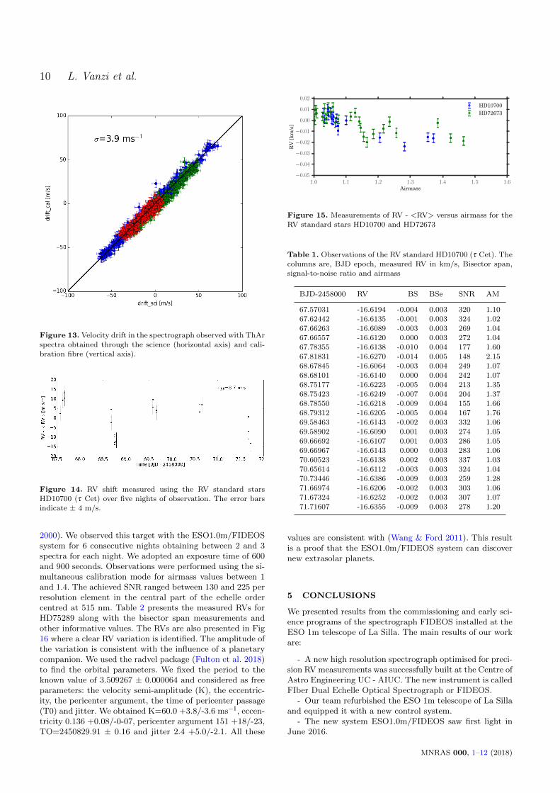
• The variations produced by changes in pressure duringour experiment were relatively smooth. Under these con-ditions the use of the comparison fiber can be trusted asa tracer of the instrumental stability for measuring preciseRVs. Figure 13 shows the drift produced on the calibrationfiber as a function of the corresponding drift in the sciencefiber, where a strong 1:1 correlation can be identified. Weobtained that this correlation presents an rms of 3.9 ms−1,which is fully consistent with the error obtained for the wave-length solution, proving again the RV limit of ∼4 ms−1.

• For the two first nights of our experiment we startedthe acquisition of the spectra immediately after switchingon the ThAr lamp. For these nights we can identify a sys-tematic offset for the instrumental drift computed with bothfibres in the case of the first ∼10 images. This shows thatfor achieving the ∼4 ms−1 stability in RV it is necessaryto wait for the stabilisation of the lamp before starting theobservations. The stabilisation of the ThAr lamp is reachedafter ≈600s.

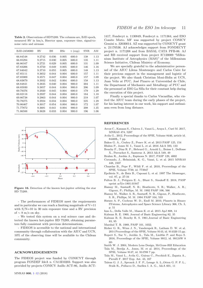
Additionally, we tested the stability of the system byobserving the radial velocity standard star HD10700. Weperformed between 3 and 5 observations per night for a to-tal number of 5 consecutive nights. We adopted an exposuretime of 180s. The observations were performed using the si-multaneous calibration mode for airmass values between 1and 1.7. The achieved SNR ranged between 150 and 340 perresolution element in the central part of the echelle ordercentred at 515 nm. The error on the RV expected for thesevalues of SNR was calculated as described in (Brahm et al.2017) and it is < 2 m/s. Table 1 presents the measured RVsand bisector spans. The RV time series is presented in figure14. The RVs present a rms of 8.7 m/s. While this preci-sion is enough for detecting giant extrasolar planets, it isstill larger that the lower stability limit of 4.0 m/s obtainedfrom the error in the wavelength solution and in the scatterof the instrumental drift by the comparison fiber. The originof the increased scatter for the measurements obtained onthe sky can be produced by atmospheric dispersion, basi-cally because the blue-to-red balance of the light enteringthe spectrograph is affected when observing at relativelyhigh airmasses. We do not employ an atmospheric disper-sion corrector. Bouchy et al. (2013) show that atmosphericdispersion can produce systematic offsets in RV as large asa few m/s. To test the effect in more detail we obtained ob-servations of the RV standard stars HD10700 and HD 72673in a range of air masses between 1 and 2. The observationsobtained with AM < 1.1 gave an RMS dispersion of 5 m/sec,close to the best expected value. However, when includingall measurements the RMS was about 10 m/s. These resultsare shown in Fig. 15.

4 EARLY SCIENCE RESULTS

The main scientific motivation of FIDEOS is the detectionand confirmation of exoplanets by measuring precision RVs.To prove the scientific potential of the instrument we ob-served the known exoplanet system HD75289, which corre-sponds to a non-transiting hot Jupiter (P=3.5 d, Mpsini =0.47 MJ) orbiting a bright (V=6.4) G0V star (Udry et al.

MNRAS 000, 1–12 (2018)

FIDEOS at the ESO 1m telescope 9

5 6 7 8 9 10 11−80−60−40−20

020406080

100

drif

t[m

/s]

3 4 5 6 7 8−50

−40

−30

−20

−10

0

10

20

drif

t[m

/s]

5 6 7 8 9 10 11768.0

768.5

769.0

769.5

770.0

770.5

pres

sure

[hPa

] 2017-11-16

3 4 5 6 7 8768.2768.3768.4768.5768.6768.7768.8768.9769.0769.1

pres

sure

[hPa

]

2017-11-19

4 5 6 7 8 9 10−60

−40

−20

0

20

40

60

80

drif

t[m

/s]

6 7 8 9 10 11−40

−20

0

20

40

60

80

100

drif

t[m

/s]

4 5 6 7 8 9 10767.4767.6767.8768.0768.2768.4768.6768.8769.0769.2

pres

sure

[hPa

]

2017-11-17

6 7 8 9 10 11768.2

768.4

768.6

768.8

769.0

769.2

769.4

769.6

769.8

pres

sure

[hPa

]

2017-11-20

7 8 9 10 11 12 13−20

0

20

40

60

80

100

drif

t[m

/s]

3 4 5 6 7 8−140−120−100−80−60−40−20

02040

drif

t[m

/s]

7 8 9 10 11 12 13time [h]

767.0

767.5

768.0

768.5

769.0

pres

sure

[hPa

]

2017-11-18

3 4 5 6 7 8time [h]

769.0

769.5

770.0

770.5

771.0

771.5

pres

sure

[hPa

]

2017-11-21

Figure 12. Velocity drift in the spectrograph observed with ThAr spectra obtained through the science (red) and calibration fibre (blue)

during 6 different nights. The continuous line represents the atmospheric pressure as measured by the ESO La Silla metro station duringthe tests. The calibration fiber has higher SNR because it is illuminated through a much shorter optical path and receives a higher signal.

MNRAS 000, 1–12 (2018)

10 L. Vanzi et al.

Figure 13. Velocity drift in the spectrograph observed with ThAr

spectra obtained through the science (horizontal axis) and cali-

bration fibre (vertical axis).

Figure 14. RV shift measured using the RV standard starsHD10700 (τ Cet) over five nights of observation. The error bars

indicate ± 4 m/s.

2000). We observed this target with the ESO1.0m/FIDEOSsystem for 6 consecutive nights obtaining between 2 and 3spectra for each night. We adopted an exposure time of 600and 900 seconds. Observations were performed using the si-multaneous calibration mode for airmass values between 1and 1.4. The achieved SNR ranged between 130 and 225 perresolution element in the central part of the echelle ordercentred at 515 nm. Table 2 presents the measured RVs forHD75289 along with the bisector span measurements andother informative values. The RVs are also presented in Fig16 where a clear RV variation is identified. The amplitude ofthe variation is consistent with the influence of a planetarycompanion. We used the radvel package (Fulton et al. 2018)to find the orbital parameters. We fixed the period to theknown value of 3.509267 ± 0.000064 and considered as freeparameters: the velocity semi-amplitude (K), the eccentric-ity, the pericenter argument, the time of pericenter passage(T0) and jitter. We obtained K=60.0 +3.8/-3.6 ms−1, eccen-tricity 0.136 +0.08/-0-07, pericenter argument 151 +18/-23,TO=2450829.91 ± 0.16 and jitter 2.4 +5.0/-2.1. All these

1.0 1.1 1.2 1.3 1.4 1.5 1.6Airmass

−0.05

−0.04

−0.03

−0.02

−0.01

0.00

0.01

0.02

RV

[km

/s]

HD10700HD72673

Figure 15. Measurements of RV - <RV> versus airmass for the

RV standard stars HD10700 and HD72673

Table 1. Observations of the RV standard HD10700 (τ Cet). The

columns are, BJD epoch, measured RV in km/s, Bisector span,

signal-to-noise ratio and airmass

BJD-2458000 RV BS BSe SNR AM

67.57031 -16.6194 -0.004 0.003 320 1.10

67.62442 -16.6135 -0.001 0.003 324 1.02

67.66263 -16.6089 -0.003 0.003 269 1.0467.66557 -16.6120 0.000 0.003 272 1.04

67.78355 -16.6138 -0.010 0.004 177 1.60

67.81831 -16.6270 -0.014 0.005 148 2.1568.67845 -16.6064 -0.003 0.004 249 1.07

68.68101 -16.6140 0.000 0.004 242 1.07

68.75177 -16.6223 -0.005 0.004 213 1.3568.75423 -16.6249 -0.007 0.004 204 1.37

68.78550 -16.6218 -0.009 0.004 155 1.66

68.79312 -16.6205 -0.005 0.004 167 1.7669.58463 -16.6143 -0.002 0.003 332 1.06

69.58902 -16.6090 0.001 0.003 274 1.05

69.66692 -16.6107 0.001 0.003 286 1.0569.66967 -16.6143 0.000 0.003 283 1.06

70.60523 -16.6138 0.002 0.003 337 1.0370.65614 -16.6112 -0.003 0.003 324 1.04

70.73446 -16.6386 -0.009 0.003 259 1.28

71.66974 -16.6206 -0.002 0.003 303 1.0671.67324 -16.6252 -0.002 0.003 307 1.07

71.71607 -16.6355 -0.009 0.003 278 1.20

values are consistent with (Wang & Ford 2011). This resultis a proof that the ESO1.0m/FIDEOS system can discovernew extrasolar planets.

5 CONCLUSIONS

We presented results from the commissioning and early sci-ence programs of the spectrograph FIDEOS installed at theESO 1m telescope of La Silla. The main results of our workare:

- A new high resolution spectrograph optimised for preci-sion RV measurements was successfully built at the Centre ofAstro Engineering UC - AIUC. The new instrument is calledFIber Dual Echelle Optical Spectrograph or FIDEOS.

- Our team refurbished the ESO 1m telescope of La Sillaand equipped it with a new control system.

- The new system ESO1.0m/FIDEOS saw first light inJune 2016.

MNRAS 000, 1–12 (2018)

FIDEOS at the ESO 1m telescope 11

Table 2. Observations of HD75289. The columns are, BJD epoch,measured RV in km/s, Bisector span, exposure time, signal-to-

noise ratio and airmass

BJD-2458000 RV BS BSe t (exp) SNR AM

66.84548 9.2742 0.036 0.005 600.0 138 1.1366.85294 9.2715 0.030 0.005 600.0 135 1.11

66.86167 9.2721 0.029 0.005 600.0 131 1.09

67.83206 9.3750 0.049 0.005 600.0 146 1.1667.84042 9.3710 0.055 0.005 600.0 148 1.13

67.85111 9.3652 0.044 0.004 600.0 157 1.11

67.85909 9.3571 0.047 0.004 600.0 157 1.0968.83879 9.3932 0.042 0.004 600.0 158 1.13

68.84841 9.3835 0.040 0.004 900.0 204 1.1168.85930 9.3857 0.044 0.004 900.0 206 1.09

69.79376 9.2920 0.045 0.004 600.0 179 1.29

69.82118 9.2937 0.044 0.004 600.0 184 1.1869.86738 9.2863 0.044 0.004 900.0 218 1.07

70.79275 9.2924 0.034 0.004 900.0 225 1.29

70.86467 9.3017 0.054 0.004 900.0 172 1.0771.77872 9.3681 0.041 0.004 900.0 208 1.35

71.86588 9.3628 0.033 0.004 900.0 196 1.06

Figure 16. Detection of the known hot-jupiter orbiting the starHD 75289.

- The performances of FIDEOS meet the requirementsand in particular we can reach a limiting magnitude of V=11with S/N=10 in 30 min exposure time and a RV precisionof ∼ 8 m/s on sky.

- We tested this system on a real science case and de-tected the known hot-jupiter HD 75289, obtaining parame-ters fully consistent with previous determinations.

- FIDEOS is accessible to the national and internationalcommunity through collaboration with the AIUC and UCN,10% of the observing time will be available to the Chileancommunity.

ACKNOWLEDGEMENTS

The FIDEOS project was funded by CONICYT throughprogram FONDEF IdeA n. CA13I10203. Support was alsoprovided by projects CONICY Anillo ACT-86, Anillo ACT-

1417, Fondecyt n. 1130849, Fondecyt n. 1171364, and ESOComite Mixto. MF was supported by project CONICYGemini n. 32030014. AZ was supported by CONICYT grantn. 21170536. AJ acknowledges support from FONDECYTproject n. 1171208 and from BASAL CATA PFB-06. AJand RB received support from project IC120009 “Millen-nium Institute of Astrophysics (MAS)” of the MillenniumScience Initiative, Chilean Ministry of Economy.

We are specially grateful to the administrative person-nel of the AIUC Lilena Montenegro and Carlos Caire fortheir precious support in the management and logistic ofthe project. We also thank Christian Moni-Bidin at UCN,Juan Veliz at PUC, Jose Pizarro at Universidad de Chile,the Department of Mechanics and Metallurgy of PUC andthe personnel at ESO La Silla for their constant help duringthe execution of this project.

Finally a special thanks to Carlos Viscasillas, who vis-ited the AIUC team during the early phases of the project,for his lasting interest in our work, his support and enthusi-asm even from long distance.

REFERENCES

Arcos C., Kanaan S., Chavez J., Vanzi L., Araya I., Cure M. 2017,

MNRAS 474, 5287

Avila G., 2012, Proceedings of the SPIE, Volume 8446, article id.84469L, 7 pp.

Bakos G. A., Csubry Z., Penev K. et al. 2013 PASP 125, 154

Bluhm P., Jones M. I., Vanzi L. et al. 2016 A&A 593, 133

Bouchy F., Diaz R. F., Hebrard G., Arnold L., Boisse I., Delfosse

X., Perruchot S., Santerne A. 2013 A&A 549, 49

Brahm R., Jordan A., Espinosa N. 2017, PASP 129, 4002

Coronado, J., Helminiak, K. G., Vanzi, L. et al. 2015 MNRAS

448, 1937

Chazelas B., Pepe F., Wildi F. et al. 2010, Proceedings of the

SPIE, Volume 7739, id. 773947

Epchtein N., de Batz B., Capoani L. et al. 1997 The Messenger,

vol. 87, p. 27-34

Fulton B. J., Petigura E. A., Blunt S., Sinukoff E. 2018, PASPeprint arXiv:1801.01947

Hamuy M., Suntzeff, N. B.; Heathcote, S. R.; Walker, A. R.;

Gigoux, P.; Phillips, M. M. 1992 PASP 106, 566

Hamuy M., Walker A. R., Suntzeff, N. B., Gigoux, P., Heathcote,

S. R., Phillips, M. M. 1994 PASP 104, 533

Hatzes A. P., Cochran W. D., Endl M. 2010, Planets in BinarySYstems, Astrophysics and Space Science Library 366, Ch. 3,

p. 51

Izzo L., Della Valle M., Mason E. et al. 2015 ApJ 808, 14

Kalman R. E. 1960, Journal of Basic Engineering 82, 35

Kalman R. E. Bouchy R. S. 1961,Journal of Basic Engineering83, 95

Marshal T. R. 1989, PASP 101, 1032;

Ricker G. R., Winn J. N., Vanderspek R., Latham D. W. et al.

2014 Proceedings of the SPIE, Volume 9143, id. 914320 15 pp.

Ropert S., Suc V., Jordan A., Tala M., Liedtke P. and Royo S.

2016, Proceedings of the SPIE, Volume 9912, id. 99124W 8pp.

Smith W. J. 2004, Modern Lens Design, McGraw-Hill Education

Tala M., Berdja A., Jones, M. et al. 2014, Proceedings of the

SPIE, Volume 9147, id. 914789 7 pp.

Tala M., Vanzi L., Avila G., Guirao C., Pecchioli E., Zapata A.,Pieralli F. 2017 Exp. Ast. 43, 167

Talens G. J. J., Spronck J. F. P., Lesage A. L.,Otten G. P. P. L.,

Stuik R., Pollacco D., Snellen I. A. G., A&A 601, 11

MNRAS 000, 1–12 (2018)

12 L. Vanzi et al.

Udry S., Mayor M., Naef D., Pepe F., Queloz D. Et al. 2000, A&A

356, 590

Vanzi L., Chacon, J., Helminiak, K. G. et al. 2012, MNRAS 424,2770

Wang J. & Ford E. B. 2011, MNRAS, 418, 1822

This paper has been typeset from a TEX/LATEX file prepared bythe author.

MNRAS 000, 1–12 (2018)