krylov methods for eigenvalue problems: theory and algorithms · outline of lecture 1 1 what is an...
TRANSCRIPT
Krylov methods for eigenvalue problems: theoryand algorithms
Karl Meerbergen
October 4-6th, 2017
Two lectures
1 Krylov methods for eigenvalue problems: theory and algorithmsI Concepts of spectral approximationI Convergence/approximation theoryI Algorithms
2 Krylov methods for eigenvalue problems: applicationsI Computing eigenvalues with largest real part (stability analysis)I Nonlinear eigenvalue problems
K. Meerbergen (KU Leuven) WSC Woudschoten October 4-6th, 2017 2 / 51

Outline of lecture 1
1 What is an eigenvalue problem?
2 Power method and friends
3 Stopping criteria
4 Matrix transformations
5 Rational Krylov sequences
6 Generalized eigenvalue problems
7 Other methods
K. Meerbergen (KU Leuven) WSC Woudschoten October 4-6th, 2017 3 / 51
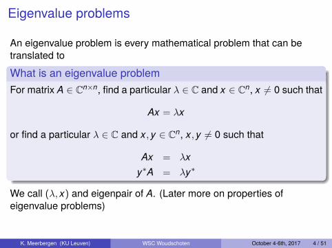
Eigenvalue problems
An eigenvalue problem is every mathematical problem that can betranslated to
What is an eigenvalue problemFor matrix A ∈ Cn×n, find a particular λ ∈ C and x ∈ Cn, x 6= 0 such that
Ax = λx
or find a particular λ ∈ C and x, y ∈ Cn, x, y 6= 0 such that
Ax = λxy∗A = λy∗
We call (λ, x) and eigenpair of A. (Later more on properties ofeigenvalue problems)
K. Meerbergen (KU Leuven) WSC Woudschoten October 4-6th, 2017 4 / 51

Power methodInitial vector x(0) with ‖x(0)‖2 = 1for k = 1,2, . . . do
y(k) = A · x(k−1)
x(k) = y(k)/‖y(k)‖2end for
Theorem (Convergence)Let the n eigenvalues λ1, . . . , λn of A be ordered as follows:
|λ1|>|λ2| ≥ · · · ≥ |λn|
(λ1 is the dominant eigenvalue; λ1 is simple.)x(k) converges to the dominant eigenvector.
Theorem (Convergence speed)The convergence rate of the dominant eigenvalue is |λ2|/|λ1|.
K. Meerbergen (KU Leuven) WSC Woudschoten October 4-6th, 2017 5 / 51
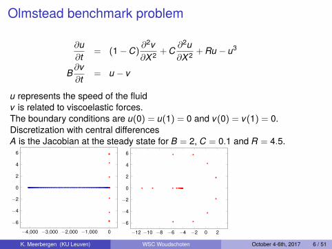
Olmstead benchmark problem
∂u∂t = (1− C)
∂2v∂X2 + C ∂2u
∂X2 + Ru − u3
B∂v∂t = u − v
u represents the speed of the fluidv is related to viscoelastic forces.The boundary conditions are u(0) = u(1) = 0 and v(0) = v(1) = 0.Discretization with central differencesA is the Jacobian at the steady state for B = 2, C = 0.1 and R = 4.5.
−4,000 −3,000 −2,000 −1,000 0
−6
−4
−2
0
2
4
6
−12 −10 −8 −6 −4 −2 0 2
−6
−4
−2
0
2
4
6
K. Meerbergen (KU Leuven) WSC Woudschoten October 4-6th, 2017 6 / 51

Shifted power methodPower on A− σI.Convergence to dominant eigenvalue of A− σI with rate ofconvergence |λ1 − σ|/|λ2 − σ|.Implementation:
(A− αI)x(k−1) = Ax(k−1) − αx(k−1)
Example (Olmstead):
−4,000 −3,000 −2,000 −1,000 0
−6
−4
−2
0
2
4
6
Shift σ = −2000.0Convergence rate: 0.99857(slow!)
K. Meerbergen (KU Leuven) WSC Woudschoten October 4-6th, 2017 7 / 51

Two friends
Subspace iterationArnoldi method (Krylov)
K. Meerbergen (KU Leuven) WSC Woudschoten October 4-6th, 2017 8 / 51
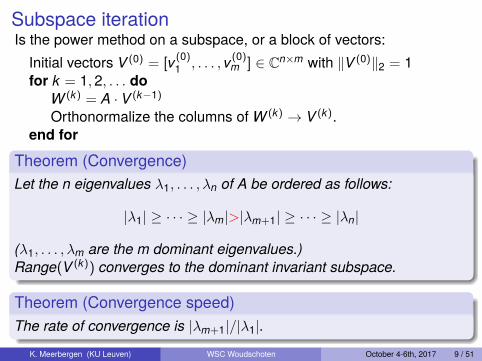
Subspace iterationIs the power method on a subspace, or a block of vectors:
Initial vectors V (0) = [v(0)1 , . . . , v(0)
m ] ∈ Cn×m with ‖V (0)‖2 = 1for k = 1,2, . . . do
W (k) = A · V (k−1)
Orthonormalize the columns of W (k) → V (k).end for
Theorem (Convergence)Let the n eigenvalues λ1, . . . , λn of A be ordered as follows:
|λ1| ≥ · · · ≥ |λm|>|λm+1| ≥ · · · ≥ |λn|
(λ1, . . . , λm are the m dominant eigenvalues.)Range(V (k)) converges to the dominant invariant subspace.
Theorem (Convergence speed)The rate of convergence is |λm+1|/|λ1|.
K. Meerbergen (KU Leuven) WSC Woudschoten October 4-6th, 2017 9 / 51

Subspace iteration
Extracting eigenvalues by Galerkin projectionx = Vz with z ∈ Cm.Galerkin:
Ax − λx ⊥ Range(V)
becomes:
V∗(Ax − λx) = = 0V∗(AVz − λVz) = 0
(V∗AV)z = λz
(V∗AV)z = λz
K. Meerbergen (KU Leuven) WSC Woudschoten October 4-6th, 2017 10 / 51

Subspace iteration
Gram-Schmidt orthogonalizationIt is very (very) important that the columns of V are orthogonalModified Gram-Schmidt is numerically unstable, i.e., columns of Vare not orthogonal to machine precisionIterative Gram-Schmidt is the solutionGram-Schmidt for orthogonalization of vector w against columnsof V :
w̃ = w − V(V∗w)v = w̃/‖w̃‖2
Iterative Gram-Schmidt is backward stable: [V , v] has orthonormalcolumns and w is spanned by the columns of [V , v].
K. Meerbergen (KU Leuven) WSC Woudschoten October 4-6th, 2017 11 / 51

Subspace iteration
Gram-Schmidt orthogonalizationIt is very (very) important that the columns of V are orthogonalModified Gram-Schmidt is numerically unstable, i.e., columns of Vare not orthogonal to machine precisionIterative Gram-Schmidt is the solutionIterative Gram-Schmidt for orthogonalization of vector w againstcolumns of V :
w̃ = w − V(V∗w)˜̃w = w̃ − V(V∗w̃)
v = ˜̃w/‖ ˜̃w‖2Iterative Gram-Schmidt is backward stable: [V , v] has orthonormalcolumns and w is spanned by the columns of [V , v].
K. Meerbergen (KU Leuven) WSC Woudschoten October 4-6th, 2017 11 / 51
Subspace iteration
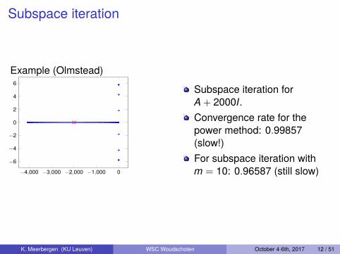
Example (Olmstead)
−4,000 −3,000 −2,000 −1,000 0
−6
−4
−2
0
2
4
6Subspace iteration forA + 2000I.Convergence rate for thepower method: 0.99857(slow!)For subspace iteration withm = 10: 0.96587 (still slow)
K. Meerbergen (KU Leuven) WSC Woudschoten October 4-6th, 2017 12 / 51
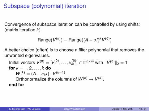
Subspace (polynomial) iteration
Convergence of subspace iteration can be controlled by using shifts:(matrix iteration k)
Range(V (k)) = Range((A− σI)kV (0))
A better choice (often) is to choose a filter polynomial that removes theunwanted eigenvalues.
Initial vectors V (0) = [v(0)1 , . . . , v(0)
m ] ∈ Cn×m with ‖V (0)‖2 = 1for k = 1,2, . . . , k do
W (k) = (A− σk I) · V (k−1)
Orthonormalize the columns of W (k) → V (k).end for
K. Meerbergen (KU Leuven) WSC Woudschoten October 4-6th, 2017 13 / 51
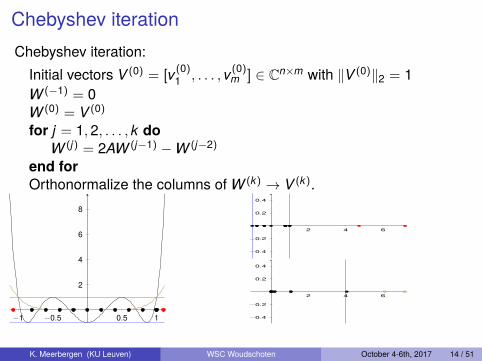
Chebyshev iterationChebyshev iteration:
Initial vectors V (0) = [v(0)1 , . . . , v(0)
m ] ∈ Cn×m with ‖V (0)‖2 = 1W (−1) = 0W (0) = V (0)
for j = 1,2, . . . , k doW (j) = 2AW (j−1) −W (j−2)
end forOrthonormalize the columns of W (k) → V (k).
−1 −0.5 0.5 1
2
4
6
8
2 4 6
−0.4
−0.2
0.2
0.4
2 4 6
−0.4
−0.2
0.2
0.4
K. Meerbergen (KU Leuven) WSC Woudschoten October 4-6th, 2017 14 / 51

Chebyshev iterationTheorem (Convergence)Let the n eigenvalues λ1, . . . , λn of A be ordered as follows:
|Tk(λ1)| ≥ · · · ≥ |Tk(λm)|>|Tk(λm+1)| ≥ · · · ≥ |Tk(λn)|
(λ1, . . . , λm are the m dominant eigenvalues of Tk(A).Range(V (k)) converges to the m eigenvalues of A outside [−1,1].The rate of convergence is |Tk(λ1)−1|.
For computing eigenvalues outside[α, β], shift and scale theChebyshev polynomial:
Tk
(A− α+β
2β−α
2
)
For complex eigenvalues:
K. Meerbergen (KU Leuven) WSC Woudschoten October 4-6th, 2017 15 / 51
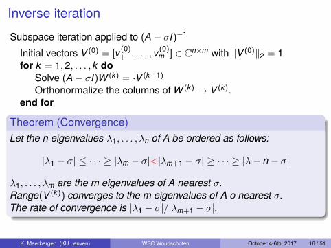
Inverse iterationSubspace iteration applied to (A− σI)−1
Initial vectors V (0) = [v(0)1 , . . . , v(0)
m ] ∈ Cn×m with ‖V (0)‖2 = 1for k = 1,2, . . . , k do
Solve (A− σI)W (k) = ·V (k−1)
Orthonormalize the columns of W (k) → V (k).end for
Theorem (Convergence)Let the n eigenvalues λ1, . . . , λn of A be ordered as follows:
|λ1 − σ| ≤ · · · ≥ |λm − σ|<|λm+1 − σ| ≥ · · · ≥ |λ− n− σ|
λ1, . . . , λm are the m eigenvalues of A nearest σ.Range(V (k)) converges to the m eigenvalues of A o nearest σ.The rate of convergence is |λ1 − σ|/|λm+1 − σ|.
K. Meerbergen (KU Leuven) WSC Woudschoten October 4-6th, 2017 16 / 51
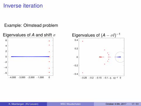
Inverse iteration
Example: Olmstead problem
Eigenvalues of A and shift σ
−4,000 −3,000 −2,000 −1,000 0
−6
−4
−2
0
2
4
6
Eigenvalues of (A− σI)−1
−0.25 −0.2 −0.15 −0.1−5 · 10−2 0−0.4
−0.2
0
0.2
0.4
K. Meerbergen (KU Leuven) WSC Woudschoten October 4-6th, 2017 17 / 51

Arnoldi methodBuild a Krylov space (from a power sequence):
{v1,Av2,A2v1, . . .Ak−1v1}
Arnoldi algorithm produces orthonormal basis Vk = [v1, . . . , vk ]:Given v1 with ‖v1‖2 = 1for j = 1, . . . , k do
wj = A · vjBlock Gram-Schmidt
hi,j = v∗i wj for i = 1, . . . , jfj = wj −
∑ji=1 vihi,j
hj+1,j = ‖fj‖2vj+1 = fj/hj+1,j
end blockend for
Eliminate wj and fj :
Avj =
j∑i=1
vihi,j + fj =
j+1∑i=1
vihi,j
K. Meerbergen (KU Leuven) WSC Woudschoten October 4-6th, 2017 18 / 51

Arnoldi method
Recurrence relations
Avj =
j∑i=1
vihi,j + fj =
j+1∑i=1
vihi,j
Define
Hk =
h1,1 h1,2 · · · h1,k
h2,1. . . ...
0 . . . ...0 hk,k−1 hk,k
∈ Ck×k
Arnoldi factorization:AVk − VkHk = fkeT
k
From V∗k Vk = I and V∗k fk = 0, we find: Hk = V∗k AVk
K. Meerbergen (KU Leuven) WSC Woudschoten October 4-6th, 2017 19 / 51

Arnoldi method
Computation of Ritz values using Galerkin projection x = Vkz:
Ax − λx ⊥ Range(Vk)
V∗k (AVkz − λVkz) = 0(V∗k AVk)z = λ(V∗k Vk)z
Hkz = z
K. Meerbergen (KU Leuven) WSC Woudschoten October 4-6th, 2017 20 / 51

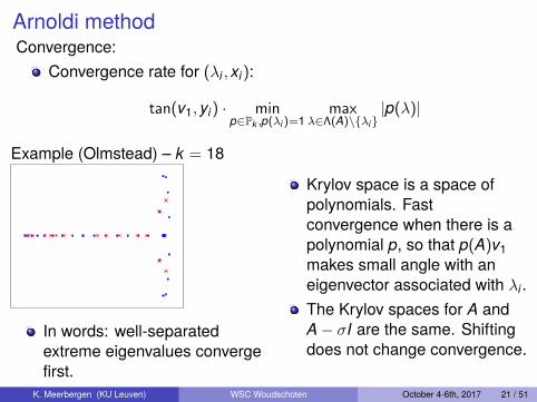
Arnoldi methodConvergence:
Convergence rate for (λi , xi):
tan(v1, yi) · minp∈Pk ,p(λi)=1
maxλ∈Λ(A)\{λi}
|p(λ)|
Example (Olmstead) – k = 10
In words: well-separatedextreme eigenvalues convergefirst.
Krylov space is a space ofpolynomials. Fastconvergence when there is apolynomial p, so that p(A)v1makes small angle with aneigenvector associated with λi .The Krylov spaces for A andA− σI are the same. Shiftingdoes not change convergence.
K. Meerbergen (KU Leuven) WSC Woudschoten October 4-6th, 2017 21 / 51

Arnoldi methodConvergence:
Convergence rate for (λi , xi):
tan(v1, yi) · minp∈Pk ,p(λi)=1
maxλ∈Λ(A)\{λi}
|p(λ)|
Example (Olmstead) – k = 11
In words: well-separatedextreme eigenvalues convergefirst.
Krylov space is a space ofpolynomials. Fastconvergence when there is apolynomial p, so that p(A)v1makes small angle with aneigenvector associated with λi .The Krylov spaces for A andA− σI are the same. Shiftingdoes not change convergence.
K. Meerbergen (KU Leuven) WSC Woudschoten October 4-6th, 2017 21 / 51

Arnoldi methodConvergence:
Convergence rate for (λi , xi):
tan(v1, yi) · minp∈Pk ,p(λi)=1
maxλ∈Λ(A)\{λi}
|p(λ)|
Example (Olmstead) – k = 12
In words: well-separatedextreme eigenvalues convergefirst.
Krylov space is a space ofpolynomials. Fastconvergence when there is apolynomial p, so that p(A)v1makes small angle with aneigenvector associated with λi .The Krylov spaces for A andA− σI are the same. Shiftingdoes not change convergence.
K. Meerbergen (KU Leuven) WSC Woudschoten October 4-6th, 2017 21 / 51

Arnoldi methodConvergence:
Convergence rate for (λi , xi):
tan(v1, yi) · minp∈Pk ,p(λi)=1
maxλ∈Λ(A)\{λi}
|p(λ)|
Example (Olmstead) – k = 13
In words: well-separatedextreme eigenvalues convergefirst.
Krylov space is a space ofpolynomials. Fastconvergence when there is apolynomial p, so that p(A)v1makes small angle with aneigenvector associated with λi .The Krylov spaces for A andA− σI are the same. Shiftingdoes not change convergence.
K. Meerbergen (KU Leuven) WSC Woudschoten October 4-6th, 2017 21 / 51

Arnoldi methodConvergence:
Convergence rate for (λi , xi):
tan(v1, yi) · minp∈Pk ,p(λi)=1
maxλ∈Λ(A)\{λi}
|p(λ)|
Example (Olmstead) – k = 14
In words: well-separatedextreme eigenvalues convergefirst.
Krylov space is a space ofpolynomials. Fastconvergence when there is apolynomial p, so that p(A)v1makes small angle with aneigenvector associated with λi .The Krylov spaces for A andA− σI are the same. Shiftingdoes not change convergence.
K. Meerbergen (KU Leuven) WSC Woudschoten October 4-6th, 2017 21 / 51

Arnoldi methodConvergence:
Convergence rate for (λi , xi):
tan(v1, yi) · minp∈Pk ,p(λi)=1
maxλ∈Λ(A)\{λi}
|p(λ)|
Example (Olmstead) – k = 15
In words: well-separatedextreme eigenvalues convergefirst.
Krylov space is a space ofpolynomials. Fastconvergence when there is apolynomial p, so that p(A)v1makes small angle with aneigenvector associated with λi .The Krylov spaces for A andA− σI are the same. Shiftingdoes not change convergence.
K. Meerbergen (KU Leuven) WSC Woudschoten October 4-6th, 2017 21 / 51

Arnoldi methodConvergence:
Convergence rate for (λi , xi):
tan(v1, yi) · minp∈Pk ,p(λi)=1
maxλ∈Λ(A)\{λi}
|p(λ)|
Example (Olmstead) – k = 16
In words: well-separatedextreme eigenvalues convergefirst.
Krylov space is a space ofpolynomials. Fastconvergence when there is apolynomial p, so that p(A)v1makes small angle with aneigenvector associated with λi .The Krylov spaces for A andA− σI are the same. Shiftingdoes not change convergence.
K. Meerbergen (KU Leuven) WSC Woudschoten October 4-6th, 2017 21 / 51

Arnoldi methodConvergence:
Convergence rate for (λi , xi):
tan(v1, yi) · minp∈Pk ,p(λi)=1
maxλ∈Λ(A)\{λi}
|p(λ)|
Example (Olmstead) – k = 17
In words: well-separatedextreme eigenvalues convergefirst.
Krylov space is a space ofpolynomials. Fastconvergence when there is apolynomial p, so that p(A)v1makes small angle with aneigenvector associated with λi .The Krylov spaces for A andA− σI are the same. Shiftingdoes not change convergence.
K. Meerbergen (KU Leuven) WSC Woudschoten October 4-6th, 2017 21 / 51
Arnoldi methodConvergence:
Convergence rate for (λi , xi):
tan(v1, yi) · minp∈Pk ,p(λi)=1
maxλ∈Λ(A)\{λi}
|p(λ)|
Example (Olmstead) – k = 18
In words: well-separatedextreme eigenvalues convergefirst.
Krylov space is a space ofpolynomials. Fastconvergence when there is apolynomial p, so that p(A)v1makes small angle with aneigenvector associated with λi .The Krylov spaces for A andA− σI are the same. Shiftingdoes not change convergence.
K. Meerbergen (KU Leuven) WSC Woudschoten October 4-6th, 2017 21 / 51

Arnoldi methodConvergence:
Convergence rate for (λi , xi):
tan(v1, yi) · minp∈Pk ,p(λi)=1
maxλ∈Λ(A)\{λi}
|p(λ)|
Example (Olmstead) – k = 19
In words: well-separatedextreme eigenvalues convergefirst.
Krylov space is a space ofpolynomials. Fastconvergence when there is apolynomial p, so that p(A)v1makes small angle with aneigenvector associated with λi .The Krylov spaces for A andA− σI are the same. Shiftingdoes not change convergence.
K. Meerbergen (KU Leuven) WSC Woudschoten October 4-6th, 2017 21 / 51

Arnoldi methodConvergence:
Convergence rate for (λi , xi):
tan(v1, yi) · minp∈Pk ,p(λi)=1
maxλ∈Λ(A)\{λi}
|p(λ)|
Example (Olmstead) – k = 20
In words: well-separatedextreme eigenvalues convergefirst.
Krylov space is a space ofpolynomials. Fastconvergence when there is apolynomial p, so that p(A)v1makes small angle with aneigenvector associated with λi .The Krylov spaces for A andA− σI are the same. Shiftingdoes not change convergence.
K. Meerbergen (KU Leuven) WSC Woudschoten October 4-6th, 2017 21 / 51
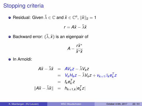
Stopping criteria
Residual: Given λ̃ ∈ C and x̃ ∈ Cn, ‖x̃‖2 = 1
r = Ax̃ − λ̃x̃
Backward error: (λ̃, x̃) is an eigenpair of
A− rx̃∗x̃∗x̃
In Arnoldi:
Ax̃ − λ̃x̃ = AVkz − λ̃Vkz= VkHkz − λ̃Vkz + vk+1βkeT
k z= fkeT
k z‖Ax̃ − λ̃x̃‖ = hk+1,k |eT
k z|
K. Meerbergen (KU Leuven) WSC Woudschoten October 4-6th, 2017 22 / 51
Matrix transformations
The Arnoldi method is faster than subspace iteration (usually), butoften still converges very slowly, in particular for large scaleproblems arising from PDEs for similar reasons as iterativemethods for linear systems of equations.The main problem:
I Memory cost: nkI Gram-Schmidt computational cost: nk2
Solutions:I Matrix transformationI Restart (as in restarted GMRES)
K. Meerbergen (KU Leuven) WSC Woudschoten October 4-6th, 2017 23 / 51
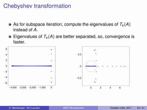
Chebyshev transformation
As for subspace iteration, compute the eigenvalues of Tk(A)instead of A.Eigenvalues of Tk(A) are better separated, so, convergence isfaster.
−4,000 −3,000 −2,000 −1,000 0
−6
−4
−2
0
2
4
6
0 2 4 6
−0.2
0
0.2
K. Meerbergen (KU Leuven) WSC Woudschoten October 4-6th, 2017 24 / 51

Shift-and-invert transformation
−4,000 −3,000 −2,000 −1,000 0
−6
−4
−2
0
2
4
6
−12 −10 −8 −6 −4 −2 0 2
−6
−4
−2
0
2
4
6
T = (A− σI)−1
The most importanttransformationBased on inverse iteration
−0.3 −0.2 −0.1 0 0.1 0.2 0.3
−0.2
0
0.2
K. Meerbergen (KU Leuven) WSC Woudschoten October 4-6th, 2017 25 / 51
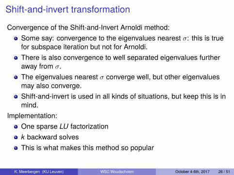
Shift-and-invert transformation
Convergence of the Shift-and-Invert Arnoldi method:Some say: convergence to the eigenvalues nearest σ: this is truefor subspace iteration but not for Arnoldi.There is also convergence to well separated eigenvalues furtheraway from σ.The eigenvalues nearest σ converge well, but other eigenvaluesmay also converge.Shift-and-invert is used in all kinds of situations, but keep this is inmind.
Implementation:One sparse LU factorizationk backward solvesThis is what makes this method so popular
K. Meerbergen (KU Leuven) WSC Woudschoten October 4-6th, 2017 26 / 51
Implicit restarting
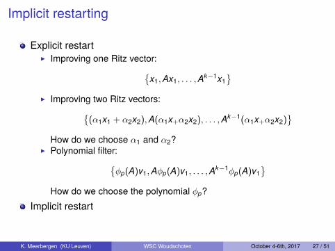
Explicit restartI Improving one Ritz vector:{
x1,Ax1, . . . ,Ak−1x1}
I Improving two Ritz vectors:{(α1x1 + α2x2),A(α1x+α2x2), . . . ,Ak−1(α1x+α2x2)
}How do we choose α1 and α2?
I Polynomial filter:{φp(A)v1,Aφp(A)v1, . . . ,Ak−1φp(A)v1
}How do we choose the polynomial φp?
Implicit restart
K. Meerbergen (KU Leuven) WSC Woudschoten October 4-6th, 2017 27 / 51

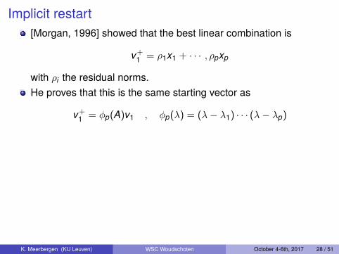
Implicit restart[Morgan, 1996] showed that the best linear combination is
v+1 = ρ1x1 + · · · , ρpxp
with ρi the residual norms.
He proves that this is the same starting vector as
v+1 = φp(A)v1 , φp(λ) = (λ− λ1) · · · (λ− λp)
[Sorensen 1992] showed that this is done by implicit restarting:1 QR factorization of QR = φp(Hk)2 Keep the first p columns of Q3 Compute V+
p = VkQ and H+p = Q∗HkQ
[M. & Spence 1997] and [Lehoucq, 1999] show that
Range(V+p ) = Range(φp(A)Vp)
(= polynomial subspace iteration)
K. Meerbergen (KU Leuven) WSC Woudschoten October 4-6th, 2017 28 / 51
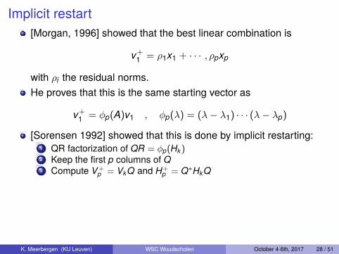
Implicit restart[Morgan, 1996] showed that the best linear combination is
v+1 = ρ1x1 + · · · , ρpxp
with ρi the residual norms.He proves that this is the same starting vector as
v+1 = φp(A)v1 , φp(λ) = (λ− λ1) · · · (λ− λp)
[Sorensen 1992] showed that this is done by implicit restarting:1 QR factorization of QR = φp(Hk)2 Keep the first p columns of Q3 Compute V+
p = VkQ and H+p = Q∗HkQ
[M. & Spence 1997] and [Lehoucq, 1999] show that
Range(V+p ) = Range(φp(A)Vp)
(= polynomial subspace iteration)
K. Meerbergen (KU Leuven) WSC Woudschoten October 4-6th, 2017 28 / 51

Implicit restart[Morgan, 1996] showed that the best linear combination is
v+1 = ρ1x1 + · · · , ρpxp
with ρi the residual norms.He proves that this is the same starting vector as
v+1 = φp(A)v1 , φp(λ) = (λ− λ1) · · · (λ− λp)
[Sorensen 1992] showed that this is done by implicit restarting:1 QR factorization of QR = φp(Hk)2 Keep the first p columns of Q3 Compute V+
p = VkQ and H+p = Q∗HkQ
[M. & Spence 1997] and [Lehoucq, 1999] show that
Range(V+p ) = Range(φp(A)Vp)
(= polynomial subspace iteration)K. Meerbergen (KU Leuven) WSC Woudschoten October 4-6th, 2017 28 / 51
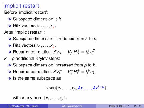
Implicit restartBefore ‘implicit restart’:
Subspace dimension is kRitz vectors x1, . . . , xp.
After ‘implicit restart’:Subspace dimension is reduced from k to p.Ritz vectors x1, . . . , xp.Recurrence relation: AV+
p − V+p H+
p = f+p eT
pk − p additional Krylov steps:
Subspace dimension increased from p to k.Recurrence relation: AV+
k − V+k H+
k = f+k eT
kIs the same subspace as
span{x1, . . . , xp,Ax, . . . ,Axk−p}
with x any from {x1, . . . , xp}.K. Meerbergen (KU Leuven) WSC Woudschoten October 4-6th, 2017 29 / 51
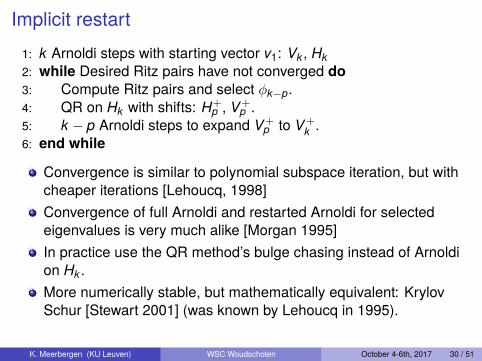
Implicit restart1: k Arnoldi steps with starting vector v1: Vk , Hk2: while Desired Ritz pairs have not converged do3: Compute Ritz pairs and select φk−p.4: QR on Hk with shifts: H+
p , V+p .
5: k − p Arnoldi steps to expand V+p to V+
k .6: end while
Convergence is similar to polynomial subspace iteration, but withcheaper iterations [Lehoucq, 1998]Convergence of full Arnoldi and restarted Arnoldi for selectedeigenvalues is very much alike [Morgan 1995]In practice use the QR method’s bulge chasing instead of Arnoldion Hk .More numerically stable, but mathematically equivalent: KrylovSchur [Stewart 2001] (was known by Lehoucq in 1995).
K. Meerbergen (KU Leuven) WSC Woudschoten October 4-6th, 2017 30 / 51

Implicit restart
Polynomial filters φk−p(λ) = (λ− σ1) · · · (λ− σk−p):
Exact shifts: shifts are Ritzvalues (Sorensen & Morgan)Chebyshev shifts: select theparameters of the Chebyshevpolynomial from the Ritzvalues and filter out the ellipsewith unwanted eigenvaluesLeja shifts (potential theory)[Calvetti, Reichel, Sorensen,1994]Zero shifts (see further)
−150 −100 −50 0
−5
0
5
K. Meerbergen (KU Leuven) WSC Woudschoten October 4-6th, 2017 31 / 51

Implicit restartMatrix is tridiagonal:
Main diagonal: 1, . . . ,1000Superdiagonal: −0.1Subdiagonal: 0.1
Arnoldi:k = 24, p = 610 sweeps of implicitrestarts are comparedto full Arnoldi with24 + 9 · 18 = 186iterations
[Morgan, 1996]K. Meerbergen (KU Leuven) WSC Woudschoten October 4-6th, 2017 32 / 51

Newton method
Apply Newton (Raphson) to:
Ax − λx = 0x∗x = 1
for (λ, x)
λ(k+1) = λ(k) + ∆λ, x(k+1 = x(k) + ∆x:[A− λ(k)I −x(k)
2(x(k))∗ 0
](∆x∆λ
)= −
(Ax(k) − λ(k)x(k)
‖x(k)‖2 − 1
)Explicitly normalize x(k) and on every iteration:
x(k+1) = −∆λ(A− λ(k)I)−1x(k)
K. Meerbergen (KU Leuven) WSC Woudschoten October 4-6th, 2017 33 / 51
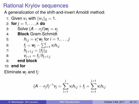
Rational Krylov sequencesA generalization of the shift-and-invert Arnoldi method:
1: Given v1 with ‖v1‖2 = 1.2: for j = 1, . . . , k do3: Solve (A− σj I)wj = vj4: Block Gram-Schmidt5: hi,j = v∗i wj for i = 1, . . . , j6: fj = wj −
∑ji=1 vihi,j
7: hj+1,j = ‖fj‖28: vj+1 = fj/hj+1,j9: end block
10: end forEliminate wj and fj :
(A− σj I)−1vj =
j∑i=1
vihi,j + fj =
j+1∑i=1
vihi,j
K. Meerbergen (KU Leuven) WSC Woudschoten October 4-6th, 2017 34 / 51
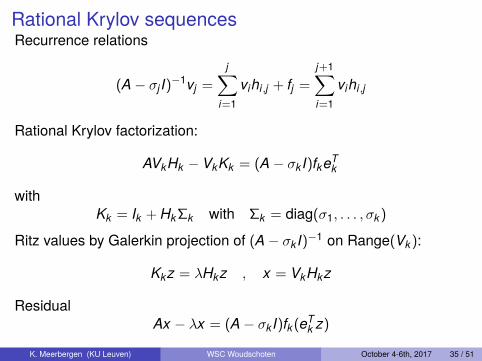
Rational Krylov sequencesRecurrence relations
(A− σj I)−1vj =
j∑i=1
vihi,j + fj =
j+1∑i=1
vihi,j
Rational Krylov factorization:
AVkHk − VkKk = (A− σk I)fkeTk
withKk = Ik + HkΣk with Σk = diag(σ1, . . . , σk)
Ritz values by Galerkin projection of (A− σk I)−1 on Range(Vk):
Kkz = λHkz , x = VkHkz
ResidualAx − λx = (A− σk I)fk(eT
k z)
K. Meerbergen (KU Leuven) WSC Woudschoten October 4-6th, 2017 35 / 51
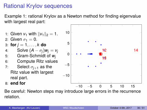
Rational Krylov sequencesExample 1: rational Krylov as a Newton method for finding eigenvaluewith largest real part:
1: Given v1 with ‖v1‖2 = 1.2: Given σ1 = 0.3: for j = 1, . . . , k do4: Solve (A− σj)wj = vj5: Gram-Schmidt of wj6: Compute Ritz values7: Select σj+1 as the
Ritz value with largestreal part.
8: end for −10 −5 0 5 10 15
−10
−5
0
5
10
01234567891011
12
13
14
Be careful: Newton steps may introduce large errors in the recurrencerelation.
K. Meerbergen (KU Leuven) WSC Woudschoten October 4-6th, 2017 36 / 51

Rational Krylov sequences
Implementation issues:Linear systems have to be solved accurately
AVkHk − BVkKk = (A− σk I)fkeTk + Rk
with ‖Rk‖ ≈ ‖(A− σj)wj − vj‖2.Linear solver is usually a direct method.Matrix factorization is often most expensive operation: reuse shiftsσj .
K. Meerbergen (KU Leuven) WSC Woudschoten October 4-6th, 2017 37 / 51
Rational Krylov sequences
Slicing for symmetric eigenvalue problem (structuraldynamics/acoustics)
K. Meerbergen (KU Leuven) WSC Woudschoten October 4-6th, 2017 38 / 51

Rational Krylov: Implicit restartingRestart with filtered starting vector/subspace:
v+1 = φk−p(A)v1 with φk−p(z) =
z − µ1z − σ1
· · · z − µk−pz − σk−p
Range(V+p ) = Range(φk−p(A)Vp)
QZ step on Hk , Kk :H+
p = Q∗HkZK +
p = Q∗KkZV+
p = VkQRecurrence relation:
AV+p H+
p − V+p K +
p = (A− σk I)f+p eT
p
The first p poles are σk−p+1, . . . , σk .Implementation:
I Naive [De Samblanx, M. & Bultheel, 1997] (including Krylov-Schur)I Bulge chasing (QZ method) [Camps, M. & Vandebril, 2017]
K. Meerbergen (KU Leuven) WSC Woudschoten October 4-6th, 2017 39 / 51

Rational Krylov: Implicit restart with zero shift
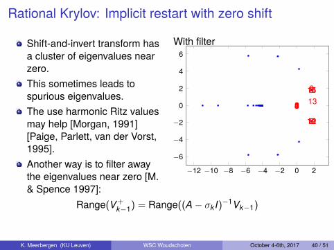
Shift-and-invert transform hasa cluster of eigenvalues nearzero.This sometimes leads tospurious eigenvalues.The use harmonic Ritz valuesmay help [Morgan, 1991][Paige, Parlett, van der Vorst,1995].Another way is to filter awaythe eigenvalues near zero [M.& Spence 1997]:
Without filter
−10 −5 0 5 10 15
−10
−5
0
5
10
01234567891011
12
13
14
Range(V+k−1) = Range((A− σk I)−1Vk−1)
K. Meerbergen (KU Leuven) WSC Woudschoten October 4-6th, 2017 40 / 51
Rational Krylov: Implicit restart with zero shift
Shift-and-invert transform hasa cluster of eigenvalues nearzero.This sometimes leads tospurious eigenvalues.The use harmonic Ritz valuesmay help [Morgan, 1991][Paige, Parlett, van der Vorst,1995].Another way is to filter awaythe eigenvalues near zero [M.& Spence 1997]:
With filter
−12 −10 −8 −6 −4 −2 0 2
−6
−4
−2
0
2
4
6
012345
67
89
101112
131415
Range(V+k−1) = Range((A− σk I)−1Vk−1)
K. Meerbergen (KU Leuven) WSC Woudschoten October 4-6th, 2017 40 / 51
Generalized eigenvalue problems
Given matrices A,B ∈ Cn×n:
Ax = λBx
Regular eigenvalue problem: A and B do not have a commonnullspace, i.e., there are α, β so that αA + βB is non-singular.
Shift-and-invert operator:
Ax = λBx(A− σB)x = (λ− σ)Bx
(λ− σ)−1x = (A− σB)−1Bx
Apply Arnoldi on (A− σB)−1B or use rational Krylov.
K. Meerbergen (KU Leuven) WSC Woudschoten October 4-6th, 2017 41 / 51

Generalized eigenvalue problems
Symmetric positive definite A and B.[Grimes, Lewis, Simon, 1994]
Choose shifts σj in between clusters of eigenvalues
(A− σB)−1B is nonsymmetric:I Use B inner product: V∗
k BVk = I.I (A− σB)−1B is self adjoint with the B-inner product:
y∗B((A− σB)−1Bx
)=((A− σB)−1By
)Bx
K. Meerbergen (KU Leuven) WSC Woudschoten October 4-6th, 2017 42 / 51

Generalized eigenvalue problemsLet B be singular and A− σB be nonsingular for some σ, then
1 for all x : Bx = 0, we have (A− σB)−1Bx = 02 which corresponds to Ax =∞Bx.
Such problems arise from DAEs (differential algebraic equations).The infinite eigenvalue is usually undesired, but it may hinder createspurious eigenvalues.Tilted plane benchmark from rational Krylov [De Samblanx, M. &Bultheel, 1997]:
Iteration Without filter With filter3 8.432 −8.46776 19.751 −9.48339 74.83 −9.48831
Implicit filtering: multiply the Krylov space with (A− σB)−1B
K. Meerbergen (KU Leuven) WSC Woudschoten October 4-6th, 2017 43 / 51

Other methods
For both right and left eigenvectors:I One Krylov space with A for right eigenvectorsI One Krylov space with A∗ for left eigenvectorsI Lanczos method, two-sided Arnoldi methodI Higher risk for spurious eigenvalues→ stabilize by an implicit
restart with zero shiftLinear systems with iterative solvers:
I Jacobi-Davidson [Sleijpen & van der Vorst]I LOBPCG [Knyazev]I Tuned preconditioner [Spence & Freitag]
Contour integral methods
K. Meerbergen (KU Leuven) WSC Woudschoten October 4-6th, 2017 44 / 51

Block Arnoldi methodArnoldi’s method applied to a block of b vectors V1 ∈ Cn×b with b > 1:
{V1,AV1,A2V1, . . .Ak−1V1}Arnoldi algorithm produces orthonormal basis Vk = [V1, . . . ,Vk ]:
Given V1 with ‖V1‖2 = 1for j = 1, . . . , k do
Wj = A · VjBlock Gram-Schmidt
for i = 1, . . . ,b doVj+1 = []Orthogonalize wj,i = Wjei against [V1, . . . ,Vj+1]Vj+1 = [Vj+1 wj,i/‖wj,i‖2]
end forend block
end forThis is like subspace iteration, where the iterations are accumulated ina subspace.
K. Meerbergen (KU Leuven) WSC Woudschoten October 4-6th, 2017 45 / 51
Two-sided Krylov methodsFor computing eigenvalues, right and left eigenvectors:
Ax = λBx y∗A = λy∗B
Two Krylov spaces(A− σB)−1B⇒ Vk ⇒ x(A∗ − σB∗)−1B∗ ⇒Wk ⇒ y
Compute Ritz triples from reduced problem:
W ∗AVz = λW ∗BVz
Lanczos method: use B bi-othogonalization: W ∗BV = I. [Bai & Ye2001]Two-sided Arnoldi method: compute projection explicitly [Ruhe ...]Implicit restarting [De Samblanx & Bultheel, 1998] for Lanczos,[Hochstenbach & Zwaan, 2017] for Arnoldi
K. Meerbergen (KU Leuven) WSC Woudschoten October 4-6th, 2017 46 / 51

Statistical approaches
K. Meerbergen (KU Leuven) WSC Woudschoten October 4-6th, 2017 47 / 51
Jacobi-Davidson method
Shift-and-invert with iterative solverIn order to avoid the need for ‘exact’ solves, JD solves thecorrection equation iteratively:
(I − yx∗/(x∗y))(A− λI)(I − xx∗/(x∗))z = −(A− λI)x
with λ = x∗Ax/(x∗x)
Preconditioning possible, but hardI prefer to solve a shifted system inexactly:
(A− σI)z = −(A− λI)x
with σ the ‘target’. The preconditioiner can be reused as long as σis not changed.
K. Meerbergen (KU Leuven) WSC Woudschoten October 4-6th, 2017 48 / 51

Locally Optimal Block Preconditioned ConjugateGradient (LOBPCG)
For symmetric Ax = λBx with positive definite Bthe Rayleigh quotient
xT AxxT Bx
is maximum for the largest eigenvalue λmax and minimum for thesmallest eigenvalue λmin
LOBPCG is the conjugate gradient method applied to thisoptimization problem
K. Meerbergen (KU Leuven) WSC Woudschoten October 4-6th, 2017 49 / 51

Contour integral methods
Let Γ ⊂ C be a closed contour in thecomplex plane.Define
Ci =
∫Γ
zi(zI − A)−1dz ∈ Cn×n
Γ
The rank of C0 is the number of eigenvalues of A inside Γ.Eigenvalue problem:
C1x = λx with C0x = x
if λ lies inside the contour.Two Methods:
I Subspace iterationI Arnoldi
K. Meerbergen (KU Leuven) WSC Woudschoten October 4-6th, 2017 50 / 51
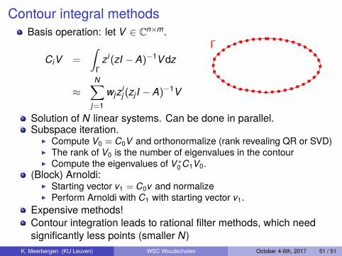
Contour integral methodsBasis operation: let V ∈ Cn×m.
CiV =
∫Γ
zi(zI − A)−1Vdz
≈N∑
j=1wjzi
j (zj I − A)−1V
Γ
Solution of N linear systems. Can be done in parallel.Subspace iteration.
I Compute V0 = C0V and orthonormalize (rank revealing QR or SVD)I The rank of V0 is the number of eigenvalues in the contourI Compute the eigenvalues of V∗
0 C1V0.(Block) Arnoldi:
I Starting vector v1 = C0v and normalizeI Perform Arnoldi with C1 with starting vector v1.
Expensive methods!Contour integration leads to rational filter methods, which needsignificantly less points (smaller N)
K. Meerbergen (KU Leuven) WSC Woudschoten October 4-6th, 2017 51 / 51