knowledge engineering for design - core · knowledge engineering for design automation phd thesis...
TRANSCRIPT

KNOWLEDGE ENGINEERING FOR DESIGN
AUTOMATION
PROEFSCHRIFT
ter verkrijging van de graad van doctoraan de Universiteit Twente,
op gezag van de rector magnificus,prof. dr. H. Brinksma,
volgens besluit van het College voor Promotiesin het openbaar te verdedigen
op vrijdag 24 april 2009 om 15.00 uur
door
Wouter Olivier Schotborghgeboren op 8 juni 1979
te Groningen

Dit proefschrift is goedgekeurd door de promotorprof. dr. ir. F.J.A.M. van Houten.
ISBN 978-90-365-2801-6
Copyright © Wouter O. Schotborgh, 2009
All rights reserved.

KNOWLEDGE ENGINEERING FOR DESIGN
AUTOMATION
PhD Thesis
By Wouter Olivier Schotborgh at the Faculty of Engineering Technology (CTW)of the University of Twente, Enschede, the Netherlands.
Enschede, 24 april 2009
De promotiecommissie:
prof. dr. F. Eising Universiteit Twente, voorzitter, secretaris
prof. dr. ir. F.J.A.M. van Houten Universiteit Twente, promotor
prof. dr. ir. A. de Boer Universiteit Twente
prof. dr. ir. O.A.M. Fisscher Universiteit Twente
prof. dr. J. van Hillegersberg Universiteit Twente
prof. D. Brissaud Grenoble Institute of Technology
prof. dr. K. Shea Technical University Munchen
prof. dr. T. Tomiyama Technische Universiteit Delft
dr. G. Still Universiteit Twente
Keywords: Knowledge Engineering, Engineering Design,Expert Knowledge, Design Automation

Aan mijn ouders,
aan Kelly


Summary
Engineering design teams face many challenges, one of which is the time pressureon the product creation process. A wide range of Information and Communica-tions Technology solutions is available to relieve the time pressure and increaseoverall efficiency. A promising type of software is that which automates a designprocess and generates design candidates, based on specifications of required be-havior. Visual presentation of multiple solutions in a “solution space” providesinsight in the trends, limitations and possibilities. This higher-level knowledgeenables the use of “design intent” and tacit experience knowledge to select thebest design for a specific application.
This thesis focuses on software support for (engineering) design processes thatuse existing technologies and knowledge, with parametric information and quan-titative data. This covers continuous and discontinuous parameters, as well as amix of linear and non-linear equations, logic and fuzzy estimations, for static anddynamic topologies. The scope includes the design of machine elements, productcomponents and product systems.
Academic research has explored the automation of design processes for a widerange of engineering problems, including the scope of this thesis. A variety oftheories, frameworks and techniques are developed to automate models of de-sign problems. Sophisticated software support is made possible with advancedfunctionalities to navigate and explore design solutions. Although the technicalfeasibility appears to be proved, the intended software support is not present inindustry to the extent that it could.
The goal of this thesis is to increase the use of design automation softwarein industrial environments. The focus lies on efficient development of the modelsthat are required for automation, with the emphasis on expert knowledge for thedesign creation phase. A method is proposed to acquire the necessary modelsand determine the software functionality. The functionality of the software isdescribed in advance to discuss the added value with the engineers that will use
VII
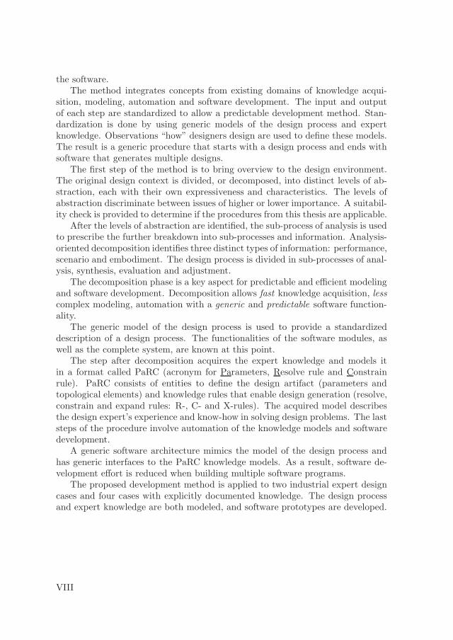
the software.The method integrates concepts from existing domains of knowledge acqui-
sition, modeling, automation and software development. The input and outputof each step are standardized to allow a predictable development method. Stan-dardization is done by using generic models of the design process and expertknowledge. Observations “how” designers design are used to define these models.The result is a generic procedure that starts with a design process and ends withsoftware that generates multiple designs.
The first step of the method is to bring overview to the design environment.The original design context is divided, or decomposed, into distinct levels of ab-straction, each with their own expressiveness and characteristics. The levels ofabstraction discriminate between issues of higher or lower importance. A suitabil-ity check is provided to determine if the procedures from this thesis are applicable.
After the levels of abstraction are identified, the sub-process of analysis is usedto prescribe the further breakdown into sub-processes and information. Analysis-oriented decomposition identifies three distinct types of information: performance,scenario and embodiment. The design process is divided in sub-processes of anal-ysis, synthesis, evaluation and adjustment.
The decomposition phase is a key aspect for predictable and efficient modelingand software development. Decomposition allows fast knowledge acquisition, lesscomplex modeling, automation with a generic and predictable software function-ality.
The generic model of the design process is used to provide a standardizeddescription of a design process. The functionalities of the software modules, aswell as the complete system, are known at this point.
The step after decomposition acquires the expert knowledge and models itin a format called PaRC (acronym for Parameters, Resolve rule and Constrainrule). PaRC consists of entities to define the design artifact (parameters andtopological elements) and knowledge rules that enable design generation (resolve,constrain and expand rules: R-, C- and X-rules). The acquired model describesthe design expert’s experience and know-how in solving design problems. The laststeps of the procedure involve automation of the knowledge models and softwaredevelopment.
A generic software architecture mimics the model of the design process andhas generic interfaces to the PaRC knowledge models. As a result, software de-velopment effort is reduced when building multiple software programs.
The proposed development method is applied to two industrial expert designcases and four cases with explicitly documented knowledge. The design processand expert knowledge are both modeled, and software prototypes are developed.
VIII

Samenvatting
Het productcreatieproces ondervindt een toenemende druk om producten van ho-ge kwaliteit in steeds kortere tijd te ontwikkelen. Informatie en CommunicatieTechnologie biedt een rijk scala aan oplossingen om de efficientie te verhogen ende concurrentie voor te blijven. Een veelbelovend type software ondersteunt hetproductcreatieproces door ontwerpalternatieven voor te stellen, op basis van ge-wenste product specificaties. Door automatisch vele alternatieve ontwerpen tegenereren en deze aan de ontwerper te presenteren wordt een “oplossingsruimte”gecreeerd. Deze oplossingsruimte biedt in een vroeg stadium van het ontwerppro-ces inzicht in de mogelijkheden en beperkingen. Dit stelt de gebruiker in staat ommet intuıtie en ervaring het beste ontwerp te kiezen voor een bepaalde toepassing.Ontwerpers besparen tijd, verhogen de kwaliteit van de uiteindelijke oplossing enverkrijgen hogere-orde kennis over de ontwerpproblematiek.
Dit proefschrift richt zich op software ondersteuning van ontwerpprocessenmet expertkennis over bestaande technologieen, met parametrische informatie enkwantitatieve getalswaarden. Hierbinnen vallen continue en discontinue varia-belen met een mix van lineaire en niet-lineaire vergelijkingen, logica en afschat-tingen, voor statische en dynamische topologieen. Het toepassingsgebied beslaatmachine-elementen, productcomponenten en productsystemen.
De academische wereld heeft automatisering van vele typen ontwerpproble-men onderzocht, onder meer voor het toepassingsgebied van dit proefschrift. Eenuitgebreide verzameling theorieen, modellen en technieken is ontwikkeld die ge-avanceerde ondersteuning mogelijk maken. Alhoewel de technische haalbaarheidlijkt te zijn aangetoond, worden automatisering van ontwerpprocessen niet veel-vuldig in de industrie toegepast.
Dit proefschrift streeft naar hogere mate van ontwerpondersteuning voor deindustrie. De focus ligt op het snel en efficient ontwikkelen van de modellen dienoodzakelijk zijn om een ontwerpproces te kunnen automatiseren. De nadrukligt op expertkennis voor de creatiefase van het ontwerpproces. Een methodische
IX

aanpak wordt beschreven om de benodigde modellen te construeren en de softwarefunctionaliteit vast te stellen.
De methode is ontwikkeld door integratie van concepten uit bestaande on-derzoeksgebieden als kennisacquisitie, modelvorming, automatisering en softwa-reontwikkeling. De gegevensuitwisseling tussen de diverse activiteiten is gestan-daardiseerd om een voorspelbare procedure te documenteren. De standaardisatiemaakt gebruik van generieke modellen van het ontwerpproces en expertkennis. Demodellen zijn opgesteld aan de hand van observaties hoe een ontwerper ontwerpten tot oplossingen komt. Het resultaat is een ontwikkelprocedure die het procesvoorschrijft van (expert)ontwerper tot en met softwaresysteem.
De eerste stap is het in kaart brengen van de ontwerpcontext. Het ontwerp-proces wordt onderverdeeld in abstractieniveaus met elk eigen informatie en pro-cessen. De abstractieniveaus verdelen het proces in zaken van hogere of lageremate van belangrijkheid. Een test wijst uit of een abstractieniveau geschikt isvoor automatisering op basis van methoden uit dit proefschrift.
Na identificatie van de abstractieniveaus, wordt deze verder verdeeld in pro-cessen en informatiesets. De analysemethode is hiervoor het centrale concept,waarbij drie typen informatie worden gedefinieerd: performance, scenario en em-bodiment. Het ontwerpproces wordt verder onderverdeeld in de processen analyse,synthese, evaluatie en aanpassen. Deze fase is de decompositie fase.
De decompositie fase is kritiek om voorspelbaar en efficient een softwarepro-gramma te kunnen ontwikkelen. Goede decompositie resulteert in snelle kennis-acquisitie en minder complexe modellen die bovendien geautomatiseerd kunnenworden met een relatief simpel algoritme dat tevens generiek toepasbaar is. Hier-door is de kernfunctionaliteit van de software in een vroeg stadium bekend.
De activiteit na decompositie is het verkrijgen en modelleren van de expertken-nis in een beschrijving genaamd PaRC (acroniem voor Parameters, Resolve-regelsen Constrain-regels). PaRC bestaat uit bouwstenen om een ontwerpobject te defi-nieren (parameters en topologische elementen) en kennisregels om ontwerpcreatiete simuleren (resolve-, constrain- en expandregels: R-, C- en X-regels).
Het kennisacquisitieproces begint met het eindresultaat van de decompositie-fase. Specifieke vragen worden aangereikt om dit proces efficient te laten verlopen.Het verkregen model beschrijft de kennis en know-how om ontwerpen te creeren.
De laatste stap van de ontwikkelprocedure beschrijft automatisering van dekennismodellen en softwareontwikkeling. Een generieke softwarearchitectuur isgebaseerd op het model van het ontwerpproces en heeft generieke interfaces naarde PaRC kennismodellen. Hierdoor wordt de vereiste inspanning om meerderesoftwaresystemen te ontwikkelen verder gereduceerd.
De beschreven ontwikkelprocedure voor ontwerpautomatisering is toegepast optwee industriele (expert)ontwerpproblemen en een viertal ontwerpproblemen diebeschreven staan in handboeken. Modellen van het ontwerpproces en expertkenniszijn opgesteld, en prototype softwareprogramma’s zijn ontwikkeld.
X
Table of Contents
Summary VII
Samenvatting IX
Table of Contents XI
1 Introduction 11.1 Software support for engineering design . . . . . . . . . . . . . . . 11.2 Solution presentation . . . . . . . . . . . . . . . . . . . . . . . . . . 21.3 Multiple solutions . . . . . . . . . . . . . . . . . . . . . . . . . . . 41.4 Software development . . . . . . . . . . . . . . . . . . . . . . . . . 61.5 Focus and scope . . . . . . . . . . . . . . . . . . . . . . . . . . . . 71.6 Research hypothesis . . . . . . . . . . . . . . . . . . . . . . . . . . 71.7 Thesis outline . . . . . . . . . . . . . . . . . . . . . . . . . . . . . . 8
2 Literature 92.1 Theory of Technical Systems . . . . . . . . . . . . . . . . . . . . . 92.2 General Design Theory . . . . . . . . . . . . . . . . . . . . . . . . . 102.3 Function-Behavior-State . . . . . . . . . . . . . . . . . . . . . . . . 102.4 Knowledge Intensive Engineering Framework . . . . . . . . . . . . 122.5 KADS and KARL . . . . . . . . . . . . . . . . . . . . . . . . . . . 132.6 Computational Synthesis . . . . . . . . . . . . . . . . . . . . . . . . 142.7 Algorithms . . . . . . . . . . . . . . . . . . . . . . . . . . . . . . . 15
2.7.1 Constraint Programming . . . . . . . . . . . . . . . . . . . 152.7.2 Optimization . . . . . . . . . . . . . . . . . . . . . . . . . . 15
2.8 MOKA . . . . . . . . . . . . . . . . . . . . . . . . . . . . . . . . . 162.9 Knowledge Engineering . . . . . . . . . . . . . . . . . . . . . . . . 172.10 Previous research . . . . . . . . . . . . . . . . . . . . . . . . . . . . 18
3 Model of synthesis knowledge 233.1 A model of design . . . . . . . . . . . . . . . . . . . . . . . . . . . 24
3.1.1 Information . . . . . . . . . . . . . . . . . . . . . . . . . . . 243.1.2 Processes . . . . . . . . . . . . . . . . . . . . . . . . . . . . 253.1.3 Levels of abstraction . . . . . . . . . . . . . . . . . . . . . . 26
XI

TABLE OF CONTENTS
3.2 What is synthesis knowledge . . . . . . . . . . . . . . . . . . . . . 273.3 A model of synthesis knowledge . . . . . . . . . . . . . . . . . . . . 29
3.3.1 Challenges . . . . . . . . . . . . . . . . . . . . . . . . . . . 293.3.2 Embodiment . . . . . . . . . . . . . . . . . . . . . . . . . . 303.3.3 Knowledge rules . . . . . . . . . . . . . . . . . . . . . . . . 31
3.4 Synthesis algorithm . . . . . . . . . . . . . . . . . . . . . . . . . . . 353.5 Limitations . . . . . . . . . . . . . . . . . . . . . . . . . . . . . . . 37
3.5.1 Systems of equations . . . . . . . . . . . . . . . . . . . . . . 373.5.2 Consistency and solvability . . . . . . . . . . . . . . . . . . 383.5.3 Revising decisions . . . . . . . . . . . . . . . . . . . . . . . 383.5.4 Algorithm . . . . . . . . . . . . . . . . . . . . . . . . . . . . 39
4 Knowledge engineering method 414.1 Step 1: identify levels of abstraction . . . . . . . . . . . . . . . . . 434.2 Step 2: selection . . . . . . . . . . . . . . . . . . . . . . . . . . . . 434.3 Step 3: analysis formalization . . . . . . . . . . . . . . . . . . . . . 44
4.3.1 Differences in analysis methods . . . . . . . . . . . . . . . . 454.4 Step 4: synthesis formalization . . . . . . . . . . . . . . . . . . . . 474.5 The knowledge document . . . . . . . . . . . . . . . . . . . . . . . 534.6 Limitations . . . . . . . . . . . . . . . . . . . . . . . . . . . . . . . 53
5 Software development method 555.1 Step 1: overview . . . . . . . . . . . . . . . . . . . . . . . . . . . . 575.2 Step 2: selection . . . . . . . . . . . . . . . . . . . . . . . . . . . . 575.3 Step 3: modeling . . . . . . . . . . . . . . . . . . . . . . . . . . . . 575.4 Step 4: automation and implementation . . . . . . . . . . . . . . . 585.5 step 5: user interaction . . . . . . . . . . . . . . . . . . . . . . . . . 59
6 Implementation and realization 636.1 Architecture . . . . . . . . . . . . . . . . . . . . . . . . . . . . . . . 636.2 Industrial cases . . . . . . . . . . . . . . . . . . . . . . . . . . . . . 68
6.2.1 Optical chamber of an XRF spectrometer . . . . . . . . . . 686.2.2 Baggage handling system . . . . . . . . . . . . . . . . . . . 77
6.3 Explicitly documented cases . . . . . . . . . . . . . . . . . . . . . . 846.3.1 Belt drive . . . . . . . . . . . . . . . . . . . . . . . . . . . . 846.3.2 Compression spring . . . . . . . . . . . . . . . . . . . . . . 906.3.3 Extension spring . . . . . . . . . . . . . . . . . . . . . . . . 926.3.4 Torsion spring . . . . . . . . . . . . . . . . . . . . . . . . . 93
6.4 Comparison . . . . . . . . . . . . . . . . . . . . . . . . . . . . . . . 946.4.1 R-rules . . . . . . . . . . . . . . . . . . . . . . . . . . . . . 946.4.2 Parameter dependency graphs . . . . . . . . . . . . . . . . 966.4.3 Development time . . . . . . . . . . . . . . . . . . . . . . . 98
7 Conclusions & Recommendations 101
XII

TABLE OF CONTENTS
7.1 Conclusions . . . . . . . . . . . . . . . . . . . . . . . . . . . . . . . 1017.2 Recommendations . . . . . . . . . . . . . . . . . . . . . . . . . . . 105
7.2.1 Industrial decomposition . . . . . . . . . . . . . . . . . . . . 1057.2.2 Knowledge acquisition . . . . . . . . . . . . . . . . . . . . . 1057.2.3 Modeling and automation . . . . . . . . . . . . . . . . . . . 1067.2.4 Generic software development . . . . . . . . . . . . . . . . . 1067.2.5 User interaction . . . . . . . . . . . . . . . . . . . . . . . . 1077.2.6 General . . . . . . . . . . . . . . . . . . . . . . . . . . . . . 107
List of References 111
Appendices
A Synthesis knowledge 119A.1 Optical chamber . . . . . . . . . . . . . . . . . . . . . . . . . . . . 119
A.1.1 Elements and parameters . . . . . . . . . . . . . . . . . . . 119A.1.2 X-rules . . . . . . . . . . . . . . . . . . . . . . . . . . . . . 121A.1.3 R-rules . . . . . . . . . . . . . . . . . . . . . . . . . . . . . 121A.1.4 C-rules . . . . . . . . . . . . . . . . . . . . . . . . . . . . . 122
A.2 Baggage handling systems . . . . . . . . . . . . . . . . . . . . . . . 123A.2.1 Elements . . . . . . . . . . . . . . . . . . . . . . . . . . . . 123A.2.2 Parameters . . . . . . . . . . . . . . . . . . . . . . . . . . . 125A.2.3 X-rules . . . . . . . . . . . . . . . . . . . . . . . . . . . . . 128A.2.4 R-rules . . . . . . . . . . . . . . . . . . . . . . . . . . . . . 129
A.3 Compression spring . . . . . . . . . . . . . . . . . . . . . . . . . . . 130A.3.1 Parameters . . . . . . . . . . . . . . . . . . . . . . . . . . . 130A.3.2 R-rules . . . . . . . . . . . . . . . . . . . . . . . . . . . . . 131A.3.3 C-rules . . . . . . . . . . . . . . . . . . . . . . . . . . . . . 132
A.4 Extension spring . . . . . . . . . . . . . . . . . . . . . . . . . . . . 133A.4.1 Parameters . . . . . . . . . . . . . . . . . . . . . . . . . . . 133A.4.2 R-rules . . . . . . . . . . . . . . . . . . . . . . . . . . . . . 134A.4.3 C-rules . . . . . . . . . . . . . . . . . . . . . . . . . . . . . 135
A.5 Torsion spring . . . . . . . . . . . . . . . . . . . . . . . . . . . . . . 135A.5.1 Parameters . . . . . . . . . . . . . . . . . . . . . . . . . . . 135A.5.2 R-rules . . . . . . . . . . . . . . . . . . . . . . . . . . . . . 136A.5.3 C-rules . . . . . . . . . . . . . . . . . . . . . . . . . . . . . 137
XIII


List of Figures
1.1 point, path and cloud solution spaces . . . . . . . . . . . . . . . . . 21.2 software support for engineering design . . . . . . . . . . . . . . . . 31.3 online flight booking application (source: website KLM) . . . . . . 41.4 solutions for suspension design . . . . . . . . . . . . . . . . . . . . 51.5 knowledge domains and the software development . . . . . . . . . . 6
2.1 the FBPSS framework (after [56]) . . . . . . . . . . . . . . . . . . . 112.2 the FBS framework (after [16]) . . . . . . . . . . . . . . . . . . . . 122.3 compression spring designer . . . . . . . . . . . . . . . . . . . . . . 202.4 synthesis module development time . . . . . . . . . . . . . . . . . . 21
3.1 embodiment and performance (image courtesy of COMSOL Inc) . 253.2 design process . . . . . . . . . . . . . . . . . . . . . . . . . . . . . . 263.3 levels of abstraction (after [26]) . . . . . . . . . . . . . . . . . . . . 27
4.1 knowledge engineering . . . . . . . . . . . . . . . . . . . . . . . . . 424.2 three types of analysis . . . . . . . . . . . . . . . . . . . . . . . . . 464.3 tube position . . . . . . . . . . . . . . . . . . . . . . . . . . . . . . 494.4 element types for functions . . . . . . . . . . . . . . . . . . . . . . 514.5 parameter dependency graph, example . . . . . . . . . . . . . . . . 52
5.1 software development . . . . . . . . . . . . . . . . . . . . . . . . . . 565.2 requirements input, belt drive case . . . . . . . . . . . . . . . . . . 605.3 solutions representation, belt drive case . . . . . . . . . . . . . . . 61
6.1 architecture . . . . . . . . . . . . . . . . . . . . . . . . . . . . . . . 646.2 central data storage, class model . . . . . . . . . . . . . . . . . . . 656.3 synthesis module, class model . . . . . . . . . . . . . . . . . . . . . 656.4 PaRC model, class model . . . . . . . . . . . . . . . . . . . . . . . 656.5 implementation example . . . . . . . . . . . . . . . . . . . . . . . . 676.6 spectrometer and optical chamber (copyright PANalytical BV) . . 696.7 optical chamber, embodiment . . . . . . . . . . . . . . . . . . . . . 726.8 parameter dependency graph, optical chamber . . . . . . . . . . . 746.9 user interface, input . . . . . . . . . . . . . . . . . . . . . . . . . . 75
XV

LIST OF FIGURES
6.10 user interface, output . . . . . . . . . . . . . . . . . . . . . . . . . . 756.12 baggage handling system (copyright Vanderlande Industries) . . . 776.13 process flow design (PFD) . . . . . . . . . . . . . . . . . . . . . . . 786.14 PFD process . . . . . . . . . . . . . . . . . . . . . . . . . . . . . . 796.15 parameter dependency graph, baggage handling system . . . . . . 826.16 material flow diagram . . . . . . . . . . . . . . . . . . . . . . . . . 836.17 belt drive, embodiment and scenario . . . . . . . . . . . . . . . . . 856.18 parameter dependency graph, belt drive . . . . . . . . . . . . . . . 886.19 graphical user interface, belt drive . . . . . . . . . . . . . . . . . . 896.20 compression spring . . . . . . . . . . . . . . . . . . . . . . . . . . . 906.21 parameter dependency graph, compression spring . . . . . . . . . . 916.22 extension spring . . . . . . . . . . . . . . . . . . . . . . . . . . . . 926.23 torsion spring . . . . . . . . . . . . . . . . . . . . . . . . . . . . . . 936.24 R-rules versus parameters . . . . . . . . . . . . . . . . . . . . . . . 946.25 number of R-rules per parameter . . . . . . . . . . . . . . . . . . . 956.26 comparison of parameter dependency graphs . . . . . . . . . . . . 976.27 synthesis module development time . . . . . . . . . . . . . . . . . . 99
7.1 knowledge domains and software development . . . . . . . . . . . . 1057.2 alternative development procedures . . . . . . . . . . . . . . . . . . 108
A.1 optical axis . . . . . . . . . . . . . . . . . . . . . . . . . . . . . . . 121
XVI

Chapter 1Introduction
We encounter in the world around us an enormous stream of products with con-stantly changing features and appearances. It seems that a product is (re)designedfor nearly every taste, price range and user group. This trend of increasing prod-uct diversity has a profound impact on companies, teams and individuals thatdevelop these products [33].
One of the reactions is to use existing technologies instead of innovative con-cepts to develop the required diversity of high quality products at affordable prices[18]. Development teams are supplied with a flexible network of internal and ex-ternal technology sources to enable quick assimilation of existing technologies.However, this increases the time pressure on new product development becausethe same technologies are also available for the competition. Therefor, in orderto remain competitive, one must increase one’s product development efficiency.
Companies have several strategies to improve efficiency of development teams,one of which is implementation of software support for the design processes [36].The research in this thesis aims to improve the software support for the (engi-neering) design processes that use existing technologies. The subsequent sectionsdescribe the currently available software and identify possible room for improve-ment.
1.1 Software support for engineering design
The fast development of consumer markets increases the pressure on the prod-uct design process to reduce time to market [21] [34]. Uncertainties and risksare reduced where possible [1] and information and communication technology isadopted to enhance flexibility, speed and efficiency of the process [36] [17].
1

Chapter 1. Introduction
A review of the commercially available software for (engineering) design re-veals that the majority focuses on analysis, drawing and/or refining details ofestablished design concepts [49] [42] [32]. Only little software support addressesthe creation process of designs. The majority of software requires a fully defineddesign as input, which forces the engineer to plan ahead and make choices. Aftera weak point is identified by simulation, this can be corrected in a number ofways. Only little methodology is provided for guidance about what to do next.
Ullman [49] describes an ideal support system for the creation of new prod-ucts: insight is provided in the relationship between the customer wishes and theavailable product options. The search for the best design is an automated process,guided by the preferences of the engineer. Support systems generate and presentalternative solutions that give an overview of what is possible. This allows expertsto use their experience and “design intent” to select the solution that is betterthan all others.
1.2 Solution presentation
A feature to distinguish support software for engineering design is the way eachtype represents a solution space, illustrates in Figure 1.1. A single software pro-gram can be of a single type or a mix of these types.
When an engineer finishes a design, he/she can execute analysis to reveal somequality characteristics, such as strength, dynamic response or a more intuitivejudgment about aesthetics or user-friendliness. After analysis, a design is placedsomewhere on a quality scale as a single point, Figure 1.1a. The point givesvaluable information about the quality of a design, but reveals nothing aboutalternatives or what the limits are of achievable quality.
a design
quality 1
quality 2
(a) point
quality 1
quality 2
(b) path (c) cloud
quality 1
quality 2
Figure 1.1: point, path and cloud solution spaces
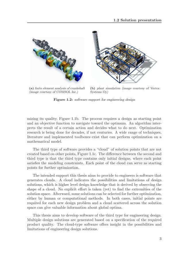
Examples of software that gives a single point solution are shown in Figure 1.2:a finite element analysis of a crankshaft predicts its mechanical behavior beforethe part is produced, Figure 1.2a. The layout of a plant is analyzed to check ifall pipes are designed correctly, Figure 1.2b. Analysis software is often essentialto deliver high quality products, meet deadlines and prevent costly redesign.
The next type of software provides information about multiple designs: eachdesign is made from a modification of a previous design, with the goal of opti-
2
1.2 Solution presentation
(a) finite element analysis of crankshaft(image courtesy of COMSOL Inc.)
(b) plant simulation (image courtesy of VertexSystems Oy)
Figure 1.2: software support for engineering design
mizing its quality, Figure 1.1b. The process requires a design as starting pointand an objective function to navigate toward the optimum. An algorithm inter-prets the result of a certain action and decides what to do next. Optimizationresearch is being done for decades, if not centuries. A wide range of techniques,literature and implemented toolboxes exist that can perform optimization on amathematical model.
The third type of software provides a “cloud” of solution points that are notcreated based on other points, Figure 1.1c. The difference between the second andthird type is that the third type contains only initial designs, where each pointsatisfies the modeling constraints. Each point of the cloud can serve as startingpoints for further optimization.
The intended support this thesis aims to provide to engineers is software thatgenerates clouds. A cloud indicates the possibilities and limitations of designsolutions, which is higher level design knowledge that is derived by observing theshape of a cloud. No explicit effort is taken (yet) to find the extremities of thesolution space. Afterward, some solutions can be selected for further optimization,either by human or computational methods. In both cases, initial points arerequired for each new design problem and a cloud scattered across the solutionspace can give valuable information about global optima.
This thesis aims to develop software of the third type for engineering design.Multiple design solutions are generated based on a specification of the requiredproduct quality. The cloud-type software offers insight in the possibilities andlimitations of engineering design solutions.
3
Chapter 1. Introduction
1.3 Multiple solutions
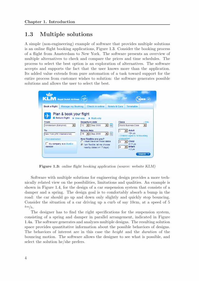
A simple (non-engineering) example of software that provides multiple solutionsis an online flight booking applications, Figure 1.3. Consider the booking processof a flight from Amsterdam to New York. The software presents an overview ofmultiple alternatives to check and compare the prices and time schedules. Theprocess to select the best option is an exploration of alternatives. The softwareaccepts and supports the fact that the user knows more than the application.Its added value extends from pure automation of a task toward support for theentire process from customer wishes to solution: the software generates possiblesolutions and allows the user to select the best.
Figure 1.3: online flight booking application (source: website KLM)
Software with multiple solutions for engineering design provides a more tech-nically related view on the possibilities, limitations and qualities. An example isshown in Figure 1.4, for the design of a car suspension system that consists of adamper and a spring. The design goal is to comfortably absorb a bump in theroad: the car should go up and down only slightly and quickly stop bouncing.Consider the situation of a car driving up a curb of say 10cm, at a speed of 5km/h.
The designer has to find the right specifications for the suspension system,consisting of a spring and damper in parallel arrangement, indicated in Figure1.4a. The software generates and analyzes multiple designs. The resulting solutionspace provides quantitative information about the possible behaviors of designs.The behaviors of interest are in this case the height and the duration of thebouncing motion. The software allows the designer to see what is possible, andselect the solution he/she prefers.
4

1.3 Multiple solutions
Figure 1.4b depicts the quantitative behavior specifications of about 200 de-signs: the overshoot on the y-axis and the settling time on the x-axis. Each dotrepresents a quantified design that is generated. The best designs are located inthe bottom-left corner (the red group).
Figure 1.4c shows a plot of the two main design variables: damping coefficientand spring coefficient. In this plot, the same group of best designs is located at theupper section of the solution cloud (the red group). Observing these two plots,the designer sees what springs and dampers will result in a comfortable ride.
The software from Figure 1.4 uses knowledge from commonly used engineeringhandbooks. However, the insight on the design solutions is difficult to obtainfrom theoretical analysis and trial-and-error iterations by hand. The softwareprovides an overview of possibilities, which saves time and ensures an optimaldesign because the designer is aware of the alternatives and picks the design thatsuits him best.
(a) (b) overshoot vs. settling time (c) design alternatives
Figure 1.4: solutions for suspension design
The software discussed in this thesis propose solutions based on knowledgerules. A list of rules is defined beforehand and an algorithm operates upon thisknowledge to find design solutions. Example of such knowledge rules are equationsand if-then logic. Knowledge from experts is used when available and acceptedas “truth”, even though the scientific rigor of such knowledge is perhaps notexplicitly researched. However, there is a growing discrepancy between softwaresupport for consumers to reduce search time and improve decision quality (e.g.route planners and online shops) and engineering design. My goal is to enablelarge scale deployment of cloud-type design automation software for present-dayengineering design.
Decades of academic research have explored many different approaches andalgorithms to realize support systems with design automation for point, path andcloud-type solution representation. Theories, frameworks and algorithms havebeen developed to enable advanced forms of intelligent, knowledge-based supportfor increasingly complex problems. The technical feasibility for a large range ofproblems within engineering design has been proved.
5

Chapter 1. Introduction
A bottleneck that begins to emerge is the development process of the softwaresystems themselves. For design problems with dynamic topologies, Cagan et al.[6] note this process is little documented. For optimization systems, Papalambrosand Wilde [31] provide a checklist and guideline for computational optimization(discussed in more detail in Section 2.7.1). The modeling is done by someone whounderstands optimization and is able to translate the design case to a computa-tional model and algorithm. Prototypes developed at my own university indicatethat different developers lead to different models with different software function-ality and require a different amount of time. My goal is to prescribe the modelingactivity as specifically as possible, leading to a more controllable process and endresult. The trade-off I will have is the applicable scope. Papalambros and Wilde[31] offer more general guidelines for a broader scope of problems, while I aim atspecific development guidelines for a more narrow scope.
1.4 Software development
A number of concepts, methods and theories from several knowledge domains arerequired during development of design automation software, Figure 1.5. The con-tinuous path through the domains, from left to right, indicates the developmentprocess of design automation software based on expert knowledge.
The development process begins with a knowledge source. The design pro-cesses of the source are first decomposed to reduce complexity, gain overview anddetermine suitable system boundaries for the software. After selection of a designprocess, the relevant knowledge is acquired and made verbally explicit. Next,the knowledge is modeled into a format that is subsequently automated by analgorithm. When developing several different software applications, the conceptof generic software development is used to reduce the required effort. Finally,the user interaction is determined to offer the best interaction and highest addedvalue for the end-user.
knowledgesource
designautomationsoftware
deco
mpo
sitio
n
know
ledg
e ac
quisition
mod
eling
auto
mat
ion
gene
ric sof
twar
e
deve
lopm
ent
user
inte
raction
Figure 1.5: knowledge domains and the software development
A development method for design automation software should be well struc-tured and documented, and have a clear applicability scope. The person to exe-cute the method is not forced to become an expert in all the knowledge domains,
6

1.5 Focus and scope
but is guided by a continuous procedure. This includes the activities from firstmeeting with the experts, to implementation of the knowledge base.
This thesis proposes a development method for design automation applica-tions and uses a model of synthesis knowledge as leading concept to integrate theknowledge domains.
1.5 Focus and scope
Software that creates many initial solutions requires, in the minimum, a modulethat creates a design and a module that analyzes a design. The act of designcreation is labeled ”synthesis”. This term is chosen to emphasize its oppositionwith analysis: synthesis begins with required specifications and results in a design,while analysis begins with a design and results in quality information. Synthesisknowledge is all information and relations that are used to generate a design. Theknowledge engineering activities to obtain the model of synthesis knowledge is thefocus of this thesis.
The scope of this thesis is engineering design that uses existing knowledgeof known technologies. The knowledge itself has parametric information andquantitative data. The source of this knowledge is available, either as humanexpert designer or explicitly documented.
1.6 Research hypothesis
The hypothesis of this thesis is:
a model of synthesis knowledge forms the basis of a knowledge engineeringmethod for the development of design automation software.
With the following definitions:� model: a simplified mathematical description of a system or process, usedto assist calculations and predictions;� knowledge engineering: the process to develop or design a computationalmodel of knowledge;� synthesis knowledge: information and relations acquired through experienceor education that are used during the synthesis phase of design: wheredesigns are generated;� design automation software: software that generates (multiple) designs.
The hypothesis is tested within the previously described scope.
7

Chapter 1. Introduction
1.7 Thesis outline
A literature survey is made to position the scope and research goal relative toexisting nomenclature and research projects. Section 3 proposes a model of thedesign process that is generic within scope and aimed at development of designautomation software. The input and output of the synthesis phase is defined anda model for the activity of synthesis proposed. A knowledge engineering methodis derived from this synthesis model to acquire and model the relevant knowledgefrom literature or human source, discussed in Section 4. How this method is usedduring software development is explained in Section 5. Chapter 6 describes theimplementation of the development method and knowledge engineering methodfor two cases from industry, and four cases from engineering handbooks. Proto-types are developed and the models of synthesis knowledge are compared to eachother. Chapter 7 concludes the thesis and proposes several future directions ofresearch.
8
Chapter 2Literature
An overview of several theories and research programs is provided to position theresearch of this thesis.
First, the Theory of Technical Systems, General Design Theory and the Function-Behavior-State model is addressed for general referencing. Next, the focus shiftsto projects of computational design support such as the framework of the Knowl-edge Intensive Engineering Framework (KIEF), the KADS research project andits more formal language KARL. Subsequently, Computational Synthesis is dis-cussed together with algorithms of Constraint Programming and optimization.The development process of design support systems is discussed by the MOKAproject and one section is dedicated to knowledge engineering. The research his-tory at the Department of Design, Production and Management of the Universityof Twente is described to illustrate the context in which this research is conducted.
2.1 Theory of Technical Systems
The Theory of Technical Systems (TTS) [19] explores the design process as broadas possible, and aims to organize, store and reference all knowledge for and aboutdesign. Central to the theory is the engineering design process to design a Techni-cal System (TS). A TS is a transformation system that is described in processes,functions, organs and components.
The lowest levels of detail are the so-called properties. These properties areall those features which belong substantially to the object. Two types of prop-erties exist: internal and external. Internal properties are under the control ofthe engineering designer, such as the structure description (components, arrange-ments), forms and dimension. The external properties are the observable anddetectable properties. In general, TTS gives a broad, qualitative description onthe relationships between properties.
9
Chapter 2. Literature
The knowledge of TTS relates the design process at enterprise level, but alsodescends in level of detail to technical knowledge: knowledge about artificial ob-jects which have been created and produced to accomplish certain goals. TTSidentifies several kinds of knowledge, such as basic knowledge about strength,materials, manufacturing, and functional knowledge about models and processes.Knowledge is available explicitly or tacitly and should always bring an answer toan immediate question.
This thesis focuses on the “property” entities of TSS and the knowledge rulesthat relate them.
2.2 General Design Theory
The General Design Theory (GDT) is a formal theory of design knowledge toclarify the human ability of designing in a scientific way [54]. It also aims toproduce practical knowledge about design methodology and the construction ofCAD systems [54].
GDT describes the design of artifacts to fulfill functions. The inputs of thedesign process are specifications, and design itself is a process of mapping thesespecifications within a functional space to an attribute space. Design is a stepwiserefinement process mediated by metamodels, toward a definite description of thedesign object in the attribute space. The attribute space is the definition of thedesign object with sufficient level of detail to be manufactured.
The theory of GDT describes design in a broad sense, while this thesis consid-ers parametric design of existing entities. In GDT terms, the software developedfrom this thesis aims to explore the neighborhood of an entity in the attributespace. Due to discontinuous degrees of freedom of the entity this might not be acontinuous space, but still relatively predictable.
2.3 Function-Behavior-State
The Function-Behavior-State concepts offer a language to describe design objectin different dimensions [50] [56]. To position this thesis, I discuss the conceptof structure as well, to explicitly differentiate between the design artifact andchanges in its attributes.
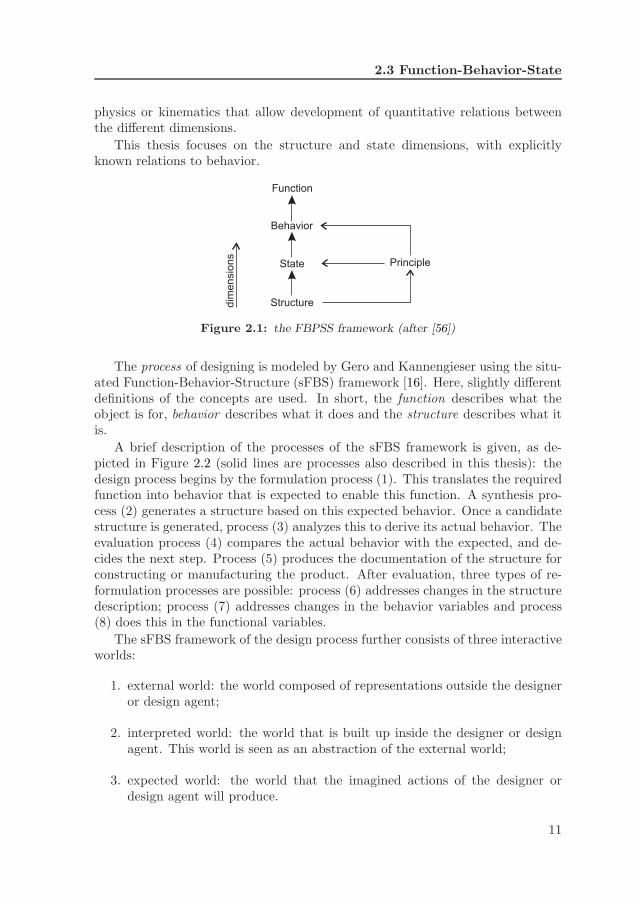
Figure 2.1 depicts the dimensions of Function, Behavior, State and Structurerelative to each other. The “lowest” dimension is the structure of the designartifact, i.e. what it is. Putting an artifact to work is described in the dimen-sion state. The states can be series of structure attributes, flows of information,material and energy. The overall relationship between these states describes thebehavior of the artifact, i.e. what it does. Finally, at the highest dimension, thebehavior is used to fulfill a certain function within a larger context.
Beside the dimensions is the concept of principle, which governs the funda-mental relations between structure, state and behavior. These are the laws of e.g.
10
2.3 Function-Behavior-State
physics or kinematics that allow development of quantitative relations betweenthe different dimensions.
This thesis focuses on the structure and state dimensions, with explicitlyknown relations to behavior.
Function
Behavior
State
Structure
Principle
dim
ensio
ns
Figure 2.1: the FBPSS framework (after [56])
The process of designing is modeled by Gero and Kannengieser using the situ-ated Function-Behavior-Structure (sFBS) framework [16]. Here, slightly differentdefinitions of the concepts are used. In short, the function describes what theobject is for, behavior describes what it does and the structure describes what itis.
A brief description of the processes of the sFBS framework is given, as de-picted in Figure 2.2 (solid lines are processes also described in this thesis): thedesign process begins by the formulation process (1). This translates the requiredfunction into behavior that is expected to enable this function. A synthesis pro-cess (2) generates a structure based on this expected behavior. Once a candidatestructure is generated, process (3) analyzes this to derive its actual behavior. Theevaluation process (4) compares the actual behavior with the expected, and de-cides the next step. Process (5) produces the documentation of the structure forconstructing or manufacturing the product. After evaluation, three types of re-formulation processes are possible: process (6) addresses changes in the structuredescription; process (7) addresses changes in the behavior variables and process(8) does this in the functional variables.
The sFBS framework of the design process further consists of three interactiveworlds:
1. external world: the world composed of representations outside the designeror design agent;
2. interpreted world: the world that is built up inside the designer or designagent. This world is seen as an abstraction of the external world;
3. expected world: the world that the imagined actions of the designer ordesign agent will produce.
11

Chapter 2. Literature
Function
ExpectedBehavior
ActualBehavior
Structure
1
2
4
3
7
8
Documentation
6
5
Figure 2.2: the FBS framework (after [16])
This thesis models a quantitative, parametric design process as an interpretedworld representation for specific, quantifiable behavior variables. Knowledge rulesare divided into the processes of synthesis, analysis, evaluation and adjustment.An explicit division is made between the artifact model and the knowledge rulesthat govern the relations between them. The link to function and documentationis outside the scope.
2.4 Knowledge Intensive Engineering Framework
The Knowledge Intensive Engineering Framework (KIEF) supports the designprocess by means of a software assistant that predicts a design object’s behaviorsacross domains [55]. KIEF integrates domain knowledge such as electronics anddynamics, allowing multi-domain analysis, causality of phenomena and qualitativereasoning about behavior.
The building blocks of KIEF are related to an ontology of physical concepts,much like geometric features. The knowledge of domain theories is related tothese physical concepts, which are stored in a library to allow for a faster andmore expressive support system. Modeling design objects in multiple domainsis done through a “metamodel”. This metamodel exists on the abstraction levelabove the domains and enables flexible integration of their knowledge theories.
First, a description of a new design object is made in different domains andconnected to the metamodel. An initial metamodel describes the design object inconceptual and topological terms. The second step involves enriching the initialmetamodel with causality knowledge to a point where the design solutions can bereasoned upon. The last step is the actual use of KIEF as a design assistant: the
12
2.5 KADS and KARL
prediction of unexpected physical phenomena across domains.
In relation to KIEF, the content of this thesis is domain agnostic. KIEFappears to focus more on the qualitative and/or causal analysis and simulationof design objects on the behavior level, while this thesis relates to the generationof design objects themselves, and the knowledge required for this.
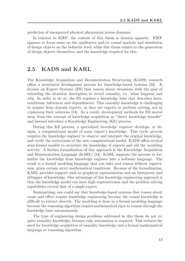
2.5 KADS and KARL
The Knowledge Acquisition and Documentation Structuring (KADS) researchoffers a structured development process for knowledge-based systems [53]. Itfocuses on Expert Systems (ES) that reason about situations with the goal ofextending the situation description to reveal causality, i.e. what happens andwhy. In order to do so, the ES requires a knowledge base that describes facts,conditions, inferences and dependencies. This causality knowledge is challengingto acquire from domain experts, as they are experts in problem solving, not inexplaining their solutions [14]. As a result, development methods for ES movedaway from the concept of knowledge acquisition as “direct knowledge transfer”and instead introduce a Knowledge Engineering (KE) process.
During this KE process, a specialized knowledge engineer develops, or de-signs, a computational model of some expert’s knowledge. This cyclic processrequires the knowledge engineer to observe and interpret the original knowledge,and verify the correctness of the new computational model. KADS offers severalsemi-formal models to structure the knowledge of experts and aid the modelingactivity. A further formalization of this approach is the Knowledge Acquisitionand Representation Language (KARL) [14]. KARL supports the process to for-malize the knowledge from knowledge engineer into a software language. Theresult is a formal modeling language that can infer and reason without supervi-sion, given certain strict mathematical conditions. Because of the formalization,KARL provides support such as graphical representation and an interpreter anddebugger of knowledge. One advantage of this knowledge engineering approach isthat the knowledge model can have high expressiveness and the problem solvingcapabilities exceed that of a single expert.
Summarizing, one could say that knowledge-based systems that reason aboutcause and effect require knowledge engineering because the causal knowledge isdifficult to extract directly. The modeling is done in a formal modeling languagebecause the reasoning algorithm require mathematical rigor to reason through theknowledge base autonomously.
The type of engineering design problems addressed in this thesis do not re-quire causality knowledge, because only automation is required. This reduces theneed for knowledge acquisition of causality knowledge and a formal mathematicallanguage or reasoning algorithm.
13
Chapter 2. Literature
2.6 Computational Synthesis
A research overview of automation and optimization of design problems withvariable topologies is given by Chakrabarti [9] and by Antonsson and Cagan [2].
The A-Design theory to computational synthesis implements an agent-basedapproach [8]. Four classes of goal-directed agents are used to generate a widerange of solutions. Configuration-agents create solutions qualitatively by randomselections of component and connect their input with output. Instantiation-agentsfix component values, determining the parameters of the design. Modificationof existing solutions is done by the fragmentation-agents. Each agent is givena preference while performing its task, resulting in a broad exploration of thesolution space. User preferences and learning algorithms from past designs areused to influence the solution generation process through manager-agents. Theseagents steer the optimization and search process by adjusting the goals of theother agents.
Computational synthesis using the A-Design theory offers support for de-sign processes ranging from shape driven (architectural) design [8] [2] to electro-mechanical systems [7]. It has also proved efficient in the travelling salespersonproblem and allows self-learning, as presented by Moss et al. [29]. A genericflowchart for computational synthesis has emerged for agent-based synthesis tools[6].
The concept of grammars offers a formalization of design synthesis knowledge.The result is a form of production rules, or graph based pattern recognitions thatexpand an initial graph into an eventual design. It supports geometric represen-tations, reasoning and emergent shape properties [2].
Within the mechanical engineering domain, a grammar is a mapping betweena function of an artifact and its form [23]. Generating solutions on both thetopological and parametric level can be done using so-called parallel grammars,e.g. for gear design [44].
Graph grammars are used for topologies, networks of elements and to representconceptual functions of a design, e.g. [43] and [23], but also neural networks [51].Because graph grammars modify a valid graph into another valid graph, eachstate can be analyzed. This enables simultaneous synthesis and optimization ine.g. MEMS design [5].
The class of design problems addressed in this thesis also have topologicaldegrees of freedom, but can be described parametrically. This thesis furtherfocuses on the generation of initial designs. Until that initial design is found, noanalysis is possible.
14

2.7 Algorithms
2.7 Algorithms
A wide range of algorithms is developed for the scope of problems I address. Thetwo groups of algorithms discussed briefly here provide a view of the wide rangeof algorithms that can be applied once a model is defined.
2.7.1 Constraint Programming
Bartak [3] provides an overview of the solving technology of Constraint Program-ming to automate design processes and generate multiple solutions. ConstraintProgramming is a method of problem solving that allows declarative specificationsof relations among objects.
For the generation of initial solutions, as intended in this thesis, the con-straint satisfaction algorithms are especially relevant, as systematic or stochasticsearch. Constraint satisfaction generates initial solutions that satisfy the con-straints, without further solution modification or optimization. Examples aregenerate-and-test, backtracking (incremental expansion), the group of consistencytechniques and constraint propagation [22].
The backtracking algorithm is a basic but robust algorithm that is likely tofind one or more solutions and is interesting to use as a baseline.
2.7.2 Optimization
Many engineering problems require not just any good solution, but the optimalsolution. Optimization algorithms generate solutions toward an optimum, definedby an objective function. Marler and Arora [24] present a survey of continuousnonlinear multi-objective optimization methods for engineering problems.
Especially relevant for software that generates multiple solutions are the Paretooptimal points: solutions that lie on the boundary of the solution space, and can-not be improved in one performance without deteriorating in another.
One of the most common methods to handle multi-objective optimization isto combine all objective functions into a single global function. Adding weights toeach individual objective allows modeling of engineering preferences. A differentapproach is the “bounded objective function method”, which offers a hierarchyin objective functions to separate between mandatory and additional objectivesthat are to be minimized.
Avoiding local optimality is important to offer a higher level interpretationof the solution space. Methods such as Tabu-search offer a heuristic procedurefor solving optimization problems, designed to guide other methods to escape thetrap of local optimality. Simulated Annealing [20] offers a stochastic optimizationprocedure to find global optima and is widely applied in optimization problems.
The scope of problems addressed in this thesis has mixed continuous and dis-continuous variables and non-linear relations of algebraic formulas and with logic.Because I aim to generate a sufficiently filled solution space, a certain amount
15
Chapter 2. Literature
of random walk in the algorithm is required. In a later stage, the algorithm cannavigate more intelligently to find the Pareto solutions, thus giving the cloudclear outlines. Exploration of the solution space would benefit from optimizationmethods to handle multi-objective optimization.
A wide range of optimization algorithms are available in literature and imple-mented for engineering problems. All these algorithms require a model to operateupon, and it is the goal of this thesis to supply the models.
2.8 MOKA
MOKA is a European research project that started in 1998 and was active for30 months. It provides a methodology to develop Knowledge-Based Engineering(KBE) applications. MOKA is an acronym for Methodology and software toolsOriented to Knowledge based engineering Applications. The goal is to reduce theinvestment and risk of KBE development: similar to this thesis. The scope isroutine design in engineering with a strong link to geometry [27].
The MOKA approach prescribes the knowledge engineering process and sup-ports it with a software tool. A standardization of knowledge was developed,called ICARE (acronym for Illustration, Constraint, Activities, Rules and Enti-ties). ICARE is divided into a part that describes the design object (constraints,entities and illustrations) and a part to describe the design process (illustrations,activities and rules). The entire process of KBE development is described asfollows:
1. knowledge gathering: collection of raw knowledge from design experts. Abroad view on the design object, processes, related aspects and backgroundinformation;
2. structuring: develop the so-called “Informal” model of knowledge, dividedinto object information and design process descriptions. The ICARE con-cepts are used to facilitate this step and the next;
3. formalizing: refine the Informal model and develop a rigorous “Formal”model of the application knowledge, that is used to build the KBE system.This model consists of two sections: the “Product Model” that describes theobject and related knowledge, and the “Design Process Model” defines theexecution and decision making order, plus the process of selection choices;
4. implementation: software development of a KBE application.
MOKA focuses on the second and third step. Software tools are developed toallow non-KBE specialists to structure and formalize the relevant knowledge usingthe ICARE concepts. The process is methodologically described in the MOKAhandbook [27].
16
2.9 Knowledge Engineering
Several commonalities and differences are identified between MOKA and thisthesis. The goals are quite similar: reduce the development effort of knowledge-based software to support the design process. But, there are also some differences.MOKA has a strong link to geometry and geometric modeling: it uses assembliesand parts explicitly. This thesis does not do this, instead it adopts conceptsof parameters and topological elements. MOKA does not prescribe the knowl-edge gathering step to determine the system boundaries and acquire the relevantknowledge. This thesis aims to do so.
MOKA’s scope is wider compared to this thesis: aiming at any engineeringdesign knowledge. Perhaps due to this wide scope, MOKA handles the solvingalgorithm (the Design Process Model) as case specific knowledge. This thesis hasa narrower scope but uses a generic solving algorithm.
2.9 Knowledge Engineering
Knowledge Engineering (KE) is the process to design or develop a computationalmodel of knowledge. KE involves activities of knowledge acquisition and repre-sentation [12] [13], both processes that have some distinct challenges.
Knowledge acquisition is the step during KE where design knowledge is madeexplicit. Schilstra [38] gives an overview of the development process of ExpertSystems, and identifies several bottlenecks still persisting. These also includethe tacit nature of expert knowledge, the challenges of knowledge extraction andthe difficulty in modeling or representing the rules. In short, the well-knownknowledge acquisition bottleneck [13].
Fensel [14] describes one of these difficulties by observing that design expertsare experts in problem solving, not in explaining their solutions. The knowl-edge engineer therefore has to obtain thorough understanding of the problemat hand. Indeed, the book “Fundamentals of Computer Aided-Engineering” byRaphael and Smith states that the most successful engineering knowledge sys-tems have been created for situations where the engineer-developers were alsowell acquainted with the subject [35].
In general, KE is seen as an activity that requires understanding of both thecomputational aspects as well as the design case at hand. The knowledge engineerhas choices to make during the representation of knowledge into rules. For thedesign of shape grammars, for instance, the ideal grammar should be compre-hensive yet model only feasible designs [2]. This involves choices regarding theamount of rules: many relatively simple ones, or a single complex rule? And thelevel of parametrization of the problem: many parameters for good expressive-ness, or fewer for better computational performance? And how to describe thedependencies that occur between the rules?
The KE activity is usually done by people who possess the knowledge. Thistrend is seen in other research projects as well. The Knowledge Acquisition andRepresentation Language (KARL [14]) is aimed at knowledge acquisition from
17

Chapter 2. Literature
the knowledge engineer into a formal language. The MOKA project addressesthe issues how to standardize and model design knowledge consistently, once it isgathered [27].
Studer et al. [45] reviews the principles and methods of knowledge engineer-ing research. The modeling activity of expert knowledge includes the process ofacquiring tacit knowledge and make this explicit. When re-usable problem solv-ing methods are used, the process of knowledge modeling is prescribed using thegeneric roles that knowledge can play. This “shell” approach is used for paramet-ric design tasks. However, the inflexibility of the problem solving method and theconnection to the real-life situations remain a challenge. A proposal is to make amore flexible, configurable set of problem solvers.
This thesis aims to prescribe the KE activities from design process decom-position, knowledge acquisition, modeling and implementation. The goal is notonly to make this process more predictable, but also for non-experts to be able toexecute it. A model of synthesis knowledge is used as leading concept to select,optimize and integrate the most appropriate ingredients from existing domains ofresearch.
The KE process addresses three major questions:
1. what is relevant: what are the system boundaries;
2. how to acquire the computational model of (synthesis) knowledge (knowl-edge acquisition);
3. how to automate the computational model: a generative algorithm.
The methods from this thesis aims to answer these three questions, without theknowledge engineer becoming a design expert him/herself. Ideally, the answers arestated by the source of the knowledge, during knowledge acquisition. The answersof the expert are implemented directly, with as little intermediate translation ormodeling by the knowledge engineer as possible.
The modeled knowledge forms the conclusion of design experts: after years ofexperience it is finally known what is important and how to generate solutionsefficiently. Using the proposed method, the knowledge is acquired and madeexplicit for the organization.
2.10 Previous research
Research projects at the Laboratory of Design, Production and Management ofthe University of Twente has been focused on intelligent design support tools fordecades. An example is the FROOM project (acronym for Features and Relationsused in Object Oriented Modeling) that supports the process of re-design, takinginto account the manufacturing and process planning aspects of design decisions[37]. Interactive features with associated knowledge are used to allow definitionand manipulation of geometry on higher levels than 3D drawing. The designer
18

2.10 Previous research
is informed of the consequences of design decisions in an early stage of design.Such functionality increases design efficiency and results in higher quality designs.The research project, of which this thesis is a part, further develops the view ofsupporting engineers to “look ahead” to see consequences of their choices and thelimitations of solution spaces.
Recent research projects explore the use of Virtual Reality (VR) during thedesign process to include the end-user in the process. Tideman [46] proposeda method that uses scenarios, VR simulations and gaming principles to supportdesigners. His method allows the different stakeholders of a design process (suchas end-users, marketing managers, maintenance specialists) to create their owndesign and immediately test these in a wide range of scenarios. This proactiverole of the stakeholders aids the designer during the design process.
The added value of VR technology is further explored in the “Synthetic En-vironments” research project (synthetic with the connotation of “artificial” or“man-made”). This project aims to provide a virtual prototyping environmentfor designers to see and feel (through haptic feedback) the implications of designdecisions. The question how to efficiently develop such an environment for a de-sign problem is among the core issues of a research project that started in 2005[28]. My research is similar in the sense that both projects aim to bring a certaintechnology to industry.
This thesis is part of the research project “Smart Synthesis Tools” that startedin 2005. The aim of this project is to provide engineering aid through automaticgeneration of design solutions. One of the first tools to explore this type ofsupport is the WATT software for mechanism design [10]. The paper by Draijerand Kokkeler discusses the seed of the philosophy that led to the “Smart SynthesisTools” (SST) project.
Research topics of the SST project address problem structuring, mathematicaltechniques, qualitative relations and handling of expert knowledge (this thesis).More details concerning the SST project are found in [41].
The question that sparked the research is related to the process of designautomation development: it is an unpredictable endeavor and the required effort isnot always in relation to its added value. To conclude this statement scientificallyrequires quantification of the development effort for a sufficiently large number ofdesign problems, in a controlled environment.
Although a number of prototypes are developed at the University of Twente[40], the scientific rigor is insufficient to draw any firm conclusions. However,we can use these prototypes to illustrate (in a non-scientific manner) the unpre-dictable nature of the development process. I estimate the development time forthe software module that performs synthesis, including knowledge acquisition,algorithm design, implementation and testing. The complexity of the synthesismodule is measured by the number of parameters that a user can optionally spec-ify as input: the degrees of freedom. The synthesis module has to cope withchanging input specifications and generate solutions that satisfy this input. Forthe data points I assume an error margin of 20 to 30%.
19
Chapter 2. Literature
First, the functionality of six prototypes is given, as well as the developmenttime of the synthesis module (not the complete application). After that, thedevelopment time is plotted against the number of degrees of freedom to illustratethe apparent lack of correlation.
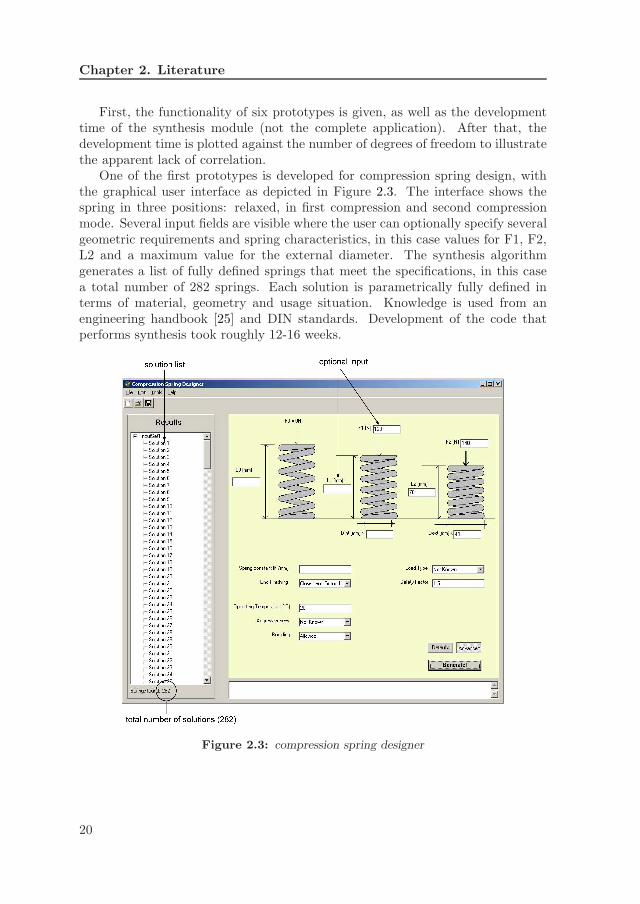
One of the first prototypes is developed for compression spring design, withthe graphical user interface as depicted in Figure 2.3. The interface shows thespring in three positions: relaxed, in first compression and second compressionmode. Several input fields are visible where the user can optionally specify severalgeometric requirements and spring characteristics, in this case values for F1, F2,L2 and a maximum value for the external diameter. The synthesis algorithmgenerates a list of fully defined springs that meet the specifications, in this casea total number of 282 springs. Each solution is parametrically fully defined interms of material, geometry and usage situation. Knowledge is used from anengineering handbook [25] and DIN standards. Development of the code thatperforms synthesis took roughly 12-16 weeks.
Figure 2.3: compression spring designer
20

2.10 Previous research
Prototypes with similar functionality as the compression spring designer aredeveloped for spindle-drives, three types of springs and fiber-reinforced compos-ites. The functionality of these prototypes is discussed briefly.
The spindle-drive designer enables the user to specify a desired motion anddynamic behavior of a manipulator that is positioned using a spindle-drive, pow-ered by an electro motor and gear transmission. The software generates severalcombinations of electro motor, transmission and spindle. The synthesis algorithmtakes into account the domains of dynamics, electronics and control systems andtook approximately 14-18 weeks to develop.
Three spring designers are developed after the first version of Figure 2.3, forcompression, extension and torsion springs. The development effort of the threesystems was reducing due to the learning effect and re-use of code: approximately10-14 weeks, 4-6 weeks and 3-5 weeks respectively.
The last prototype is the composite designer, which supports the design offiber-reinforced composites. The user can specify which materials are allowed andinformation about the orientation and stacking of the plies. Different synthesisand optimization algorithms were implemented but the first algorithm (full search)took approximately 2 weeks.
The relation between the development time and number of degrees of freedomis given in Figure 2.4. The figure illustrates the unpredictable nature of thedevelopment of the synthesis module: no apparent correlation exists between thedevelopment time and the complexity of the problem. Secondly, a developmenttime of several months only for the design generation module of a mechanicalspring seems out of proportion.
B
C
DE
A
F
0
2
4
6
8
10
12
14
16
18
0 2 4 6 8 10 12 14 16
development
�me (weeks)
degrees of freedom
D: extension springE: torsion springF: fibre reinforced composite
A: spindle driveB: compression spring (1)C: compression spring (2)
Figure 2.4: synthesis module development time
21

Chapter 3Model of synthesis
knowledge
The hypothesis of this thesis speaks of a model of synthesis that is ultimatelyintended to be automated. Such automation will simulate an act of synthesis.This chapter proposes a model of synthesis to describe this activity. The modelconsists of three parts: a description of the design artifact, a set of knowledgerules and an algorithm to combine these two and perform the act of synthesis.
From a cognitive point of view, synthesis can be seen as a construction ofrepresentations [52]. The synthesis phase starts with the design requirements andelaborates this representation toward the description of a complete design. Therole of knowledge during this activity is not completely clear, but Wittgensteinused the phrase:
“To know means to know how to go on” (Ludwig Wittgenstein)
An interpretation of Wittgenstein’s view on knowledge is that it enables the ownerto move from some begin to some end. This chapter proposes a description ofsynthesis knowledge, based on the view that knowledge enables the owner to takethe next step.
First, a model of the design process is provided to position the activity ofsynthesis within the larger context, after which a more in depth discussion onsynthesis follows.
23

Chapter 3. Model of synthesis knowledge
3.1 A model of design
A design process consists of a series of processes that starts with the requirementsand ends with a specification of a design. This section models a design process,its sub-processes and sub-sets of information. First, the sets of information areintroduced, after which the flow of this information through the sub-processes isgiven.
3.1.1 Information
The goal of a design process is to arrive at a description of a “design” that satisfiescertain requirements. Such a design does not necessarily describe geometry or aphysical product, but can also be a layout or sketch. The concept of embodimentis introduced as the representation of the design artifact or system that is beingdesigned. An embodiment can be a physical product such as a spring or machine,but also a control system or network layout. Higher level abstractions of springsor machines are represented by fewer parameters, but are still embodiments.
Embodiments are not designed to sit on a shelf doing nothing, but to beused in a certain situation. The description of such a usage situation is calleda scenario. The scenario is information a designer cannot freely change. Forinstance, a spring is being deformed and a machine is switched on. A networklayout is subjected to one or more scenarios, such as set of input signals. In caseof the design of a construction beam, a scenario is the load that it has to support,or the temperature it has to withstand. The designer can change the design ofthe beam, but not the force that it will receive. The scenario is typically dictatedfrom outside the design process, such a customer or previous design process.
After the embodiment and scenario are both known, the quality of the em-bodiment in that scenario is determined. The performance is the behavior thatan embodiment exhibits in a scenario. For example, a construction beam has in-ternal material stresses due to the load being applied, and a machine has certaindynamic performances such as overshoot and error margins.
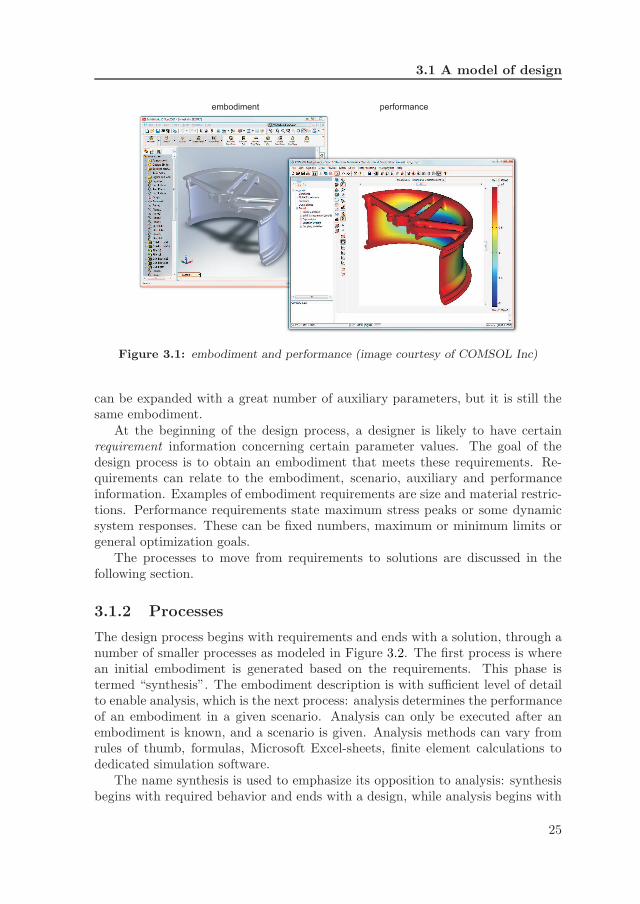
Figure 3.1 shows an example of an embodiment and performance. The em-bodiment is a geometric model of a rim. The scenario is a fixed displacement andthe performance is the resulting strain.
Because this thesis focuses on quantitative parametric designs, the embod-iment, scenario and performance are all described in quantifiable parameters:information entities that receive a value during the design process. Parameterscan be of different types, such as discrete, continuous, integers, predicates andsets (e.g. a material with a collection of properties).
In addition to the before mentioned independent types of parameters, a fourthtype is introduced to express extra (dependent) information such as design intentand temporary construction parameters: auxiliary information. Examples areratios, temporary estimates and the number of parts of an assembly. A model
24
3.1 A model of design
embodiment performance
Figure 3.1: embodiment and performance (image courtesy of COMSOL Inc)
can be expanded with a great number of auxiliary parameters, but it is still thesame embodiment.
At the beginning of the design process, a designer is likely to have certainrequirement information concerning certain parameter values. The goal of thedesign process is to obtain an embodiment that meets these requirements. Re-quirements can relate to the embodiment, scenario, auxiliary and performanceinformation. Examples of embodiment requirements are size and material restric-tions. Performance requirements state maximum stress peaks or some dynamicsystem responses. These can be fixed numbers, maximum or minimum limits orgeneral optimization goals.
The processes to move from requirements to solutions are discussed in thefollowing section.
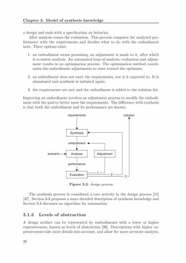
3.1.2 Processes
The design process begins with requirements and ends with a solution, through anumber of smaller processes as modeled in Figure 3.2. The first process is wherean initial embodiment is generated based on the requirements. This phase istermed “synthesis”. The embodiment description is with sufficient level of detailto enable analysis, which is the next process: analysis determines the performanceof an embodiment in a given scenario. Analysis can only be executed after anembodiment is known, and a scenario is given. Analysis methods can vary fromrules of thumb, formulas, Microsoft Excel-sheets, finite element calculations todedicated simulation software.
The name synthesis is used to emphasize its opposition to analysis: synthesisbegins with required behavior and ends with a design, while analysis begins with
25
Chapter 3. Model of synthesis knowledge
a design and ends with a specification on behavior.After analysis comes the evaluation. This process compares the analyzed per-
formance with the requirements and decides what to do with the embodimentnext. Three options exist:
1. an embodiment seems promising, an adjustment is made to it, after whichit re-enters analysis. An automated loop of analysis, evaluation and adjust-ment results in an optimization process. The optimization method coordi-nates the embodiment adjustments to steer toward the optimum;
2. an embodiment does not meet the requirements, nor is it expected to. It isabandoned and synthesis is initiated again;
3. the requirements are met and the embodiment is added to the solution list.
Improving an embodiment involves an adjustment process to modify the embodi-ment with the goal to better meet the requirements. The difference with synthesisis that both the embodiment and its performance are known.
requirements
Synthesis
Analysis
Evaluation
Adjustment
embodiment
performance
scenario
solution
1112
3
Figure 3.2: design process
The synthesis process is considered a core activity in the design process [11][47]. Section 3.3 proposes a more detailed description of synthesis knowledge andSection 3.4 discusses an algorithm for automation.
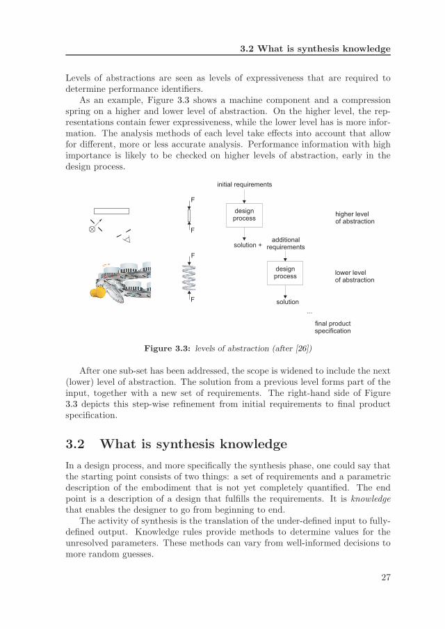
3.1.3 Levels of abstraction
A design artifact can be represented by embodiments with a lower or higherexpressiveness, known as levels of abstraction [26]. Descriptions with higher ex-pressiveness take more details into account, and allow for more accurate analysis.
26
3.2 What is synthesis knowledge
Levels of abstractions are seen as levels of expressiveness that are required todetermine performance identifiers.
As an example, Figure 3.3 shows a machine component and a compressionspring on a higher and lower level of abstraction. On the higher level, the rep-resentations contain fewer expressiveness, while the lower level has is more infor-mation. The analysis methods of each level take effects into account that allowfor different, more or less accurate analysis. Performance information with highimportance is likely to be checked on higher levels of abstraction, early in thedesign process.
initial requirements
designprocess
solution +additional
requirements
designprocess
solution
higher levelof abstraction
lower levelof abstraction
...
final productspecification
F
F
F
F
Figure 3.3: levels of abstraction (after [26])
After one sub-set has been addressed, the scope is widened to include the next(lower) level of abstraction. The solution from a previous level forms part of theinput, together with a new set of requirements. The right-hand side of Figure3.3 depicts this step-wise refinement from initial requirements to final productspecification.
3.2 What is synthesis knowledge
In a design process, and more specifically the synthesis phase, one could say thatthe starting point consists of two things: a set of requirements and a parametricdescription of the embodiment that is not yet completely quantified. The endpoint is a description of a design that fulfills the requirements. It is knowledgethat enables the designer to go from beginning to end.
The activity of synthesis is the translation of the under-defined input to fully-defined output. Knowledge rules provide methods to determine values for theunresolved parameters. These methods can vary from well-informed decisions tomore random guesses.
27

Chapter 3. Model of synthesis knowledge
After a value is determined for a parameter, a check is made to verify if theprocess is moving in the right direction. Again, knowledge provides the means tocheck if the current set of parameter values is allowed or conflicting. An allowedcombination of values describes a valid (partial) design and the next parametervalue can be resolved. If the values are conflicting, the embodiment descriptionis invalid. One possibility is go back some steps and try a different route. Thesynthesis activity is finished if all parameter values are resolved and withoutconflict.
So far, three things are needed to describe synthesis:
1. the modeling entities: parameters;
2. methods to resolve a parameter value, i.e. reduce the dimension of theproblem space: R-rules;
3. methods to limit the allowed solution space: C-rules.
This description of knowledge is labeled PaRC: Parameter, Resolve and Constrain.A relatively simple algorithm is used to simulate the activity of synthesis. Thealgorithm consists of three basic steps:
1. step forward: execute one R-rule;
2. check: execute the C-rules;
3. in case of a conflict, reverse one or several steps and try a different route.
The steps are similar to the Role-Limiting Method [45] and Backtracking fromconstraint satisfaction [22], but now explicitly defined in terms of the PaRC model.A more detailed formulation of PaRC is given in Section 3.3.
Note 1: resulting from these definitions, a difference exists between regularalgebraic equations and R-rules: Expression (3.1) is not synthesis knowledge forparameters p1 and p2.
p1 + p2 = 1 (3.1)
Equation (3.1) needs translation into either (3.2) or (3.3) before it is used to“step forward” in the synthesis process. Expressions (3.2) and (3.3) are synthesisknowledge, because they describe a method to resolve a parameter. Executingthese R-rules results in a step toward the endpoint of the synthesis process.
p1 = 1 − p2 (3.2)
p2 = 1 − p1 (3.3)
28

3.3 A model of synthesis knowledge
Note 2: please note the difference between constraints and constrain (with-out “t”). In general, constraints are all restrictions and relations a solutions hasto satisfy: both equalities and inequalities. In this thesis I separate equalities andinequalities. I do this by introducing R-rules and C-rules. The R-rules are usedto model the equalities. C-rules are the relations that limit, restrict or constrainthe allowed values of a parameter: inequalities.
3.3 A model of synthesis knowledge
Synthesis knowledge consists of a parametric embodiment model and a set ofknowledge rules that enable generation of a valid embodiment. Both topics arediscussed in more detail in the following section, and the algorithm that automatessynthesis is discussed afterward [39]. I am aware of the fact that, at some points,I slightly abuse the formal mathematical notations, but I hope this does not causeconfusion.
First, a general remark about the complexity of design automation is made,to illustrate the kind of calculations involved.
3.3.1 Challenges
Generating designs is generally an under constrained problem: there are moreunknown parameters than there are equations. Actually, having equations is al-ready a luxury. Studying design cases from engineering handbooks and industrialsettings shows a mix of linear and non-linear algebraic equations, logic reasoningand random estimations. These relations can come from scientific formulas orfuzzy experience knowledge. Choices made earlier can influence what rules toapply later on. Designs with topological freedom can include or exclude entiregroups of variables and relations. From a mathematical point of view, automatingsuch a problem in a generic manner is not straight forward.
The parameters that describe a design are a mix of continuous and discontin-uous, booleans and set-based parameters. For example, the parameter “material”is composed of a Young’s module, density and melting temperature. One cannotuse an equation to determine a value for the Young’s module: such a material isnot guaranteed to exist.
Another challenge with automating synthesis is the unpredictable input infor-mation. The user might, or might not, prescribes the value of certain parameters.And this can change each time the software is used. The algorithm could en-counter systems of equations, or worse: a system of relations with all the mixedtypes described earlier. And in advance one does not know if a solution exists ornot. In any case, the algorithm that performs synthesis has to complete the restof the design automatically and find solutions, if they exist.
In summary, automating synthesis is a complex problem. Fortunately, thereis a bright side: humans can do it. A human designer is able to generate solutions
29
Chapter 3. Model of synthesis knowledge
for the problem described above. This might sound trivial, but has an importantconsequence for the definition of synthesis knowledge and the algorithm proposedin Section 3.4.
3.3.2 Embodiment
An embodiment is modeled as a collection of parameters p ∈ P . Parametersthat belong together are grouped within elements e ∈ E, so that the element“compression spring” is described by parameters such as material, wire thicknessand length. Each parameter within an element is unique.
Each element e ∈ E is an instantiation of an element type t ∈ T . All elementsthat are used during synthesis are first defined as an element type. Separatetypes exist for cog wheels, levers, springs and so on. During synthesis, multipleelement of the same element type are allowed, e.g. two compression springs in onemachine. Both elements are of the same type (i.e. compression spring) but havedifferent instances. Although these elements have the same parameters, theseparameters can have different values.
The parameter values of element e are represented by the following vector:
ve(p) p ∈ Pe (3.4)
At creation of the element, the value is unknown. During synthesis, its valuebecomes resolved. The notion for the value being unknown or known is denotedas:
ve(p)
{
= λ if ve(p) is not yet known
6= λ if ve(p) is known(3.5)
Once a parameter is resolved, its value can be valid or invalid. The C-rulesdetermine the allowed solution space cp for parameter p. The solution space cp isformed by the C-rules that apply to parameter p and depend on ve(p) 6= λ, i.e.all C-rules that can be executed to constrain the solution space.
Section 3.3.3 discusses how these parameters receive their values and how thesolution space is determined.
Topology
A topology of the embodiment resembles the product structure. The topology isdefined as a hierarchical tree of elements e ∈ E, with E ⊂ T . During generation ofa topology, each element e is expanded with a (possibly empty) set of sub-elementsse ⊂ T . The rules that prescribe the addition of sub-elements are termed X-rules.The X-rule changes the state of the sub-elements, denoted as:
se
{
= λ if se is not yet known
6= λ if se is known(3.6)
30

3.3 A model of synthesis knowledge
These sets of sub-elements have to respect the normal tree semantics, i.e. noelement can be its own sub-element, neither directly, nor indirectly. Furthermore,each element has a unique super-element, except for a single root element thatrepresents the complete design. A (partial) embodiment is thus represented bythe set of elements E, their hierarchical structure s and the parameters values v,denoted as vector (E, v, s).
Solution
A solution for the synthesis phase is an embodiment that satisfies the followingconditions:
se 6= λ ∀e ∈ E (3.7)
ve(p) 6= λ ∀e ∈ E, p ∈ Pe (3.8)
ve(p) ⊂ cp ∀e ∈ E, p ∈ Pe (3.9)
I.e. the topology is fully expanded (3.7), no parameter value is unresolved forany element (3.8) and each parameter value lies within the allowed set, for eachelement (3.9).
3.3.3 Knowledge rules
The synthesis knowledge is organized using the object-oriented paradigm [4],where the objects are parameter p ∈ P and element type t ∈ T . This meansthat parameters and element types are self sustaining entities, or agents, withtheir own knowledge rules. It is important to note that these rules are the samefor every instantiated element e from t, i.e. two compression springs possess thesame knowledge.
The general structure of a knowledge rules is as follows:� object(s): the parameter(s) or element type(s) to operate upon;� conditional set: the set of parameters that is required to have a value beforethe rule can be executed;� action: the explicitly described operation on the object(s).
Three types of knowledge rules exist: X-, R- and C-rules. The rules are discussedin more detail in the following section, each with a pseudo-code example.
Note: as mentioned before, please note the difference between constraints(with “t”) and constrain (without “t”). In general, constraints are all restrictionsand relations a solutions has to satisfy: both equalities and inequalities. In thisthesis I separate equalities and inequalities. I do this by introducing R-rules andC-rules. The R-rules are used to model the equalities. C-rules are the relationsthat limit, restrict or constrain the allowed values of a parameter: inequalities.
31

Chapter 3. Model of synthesis knowledge
X-rules Xt An element type t ∈ T contains the knowledge to add sub-elements. X-rules expand the hierarchy of elements by transforming a partialembodiment (E, v, s) into a new partial embodiment (E′, v′, s′). This is done bydetermining the set of sub-elements s′e for an element e ∈ E for which se = λ andadding these elements to E to form E′. A single X-rule can add multiple typesof elements, or multiple instances of the same element type.
Example An example of an X-rule is the topological expansion of elementE1 with N element instances E2 from element type ET2. In addition, the param-eter thickness of the sub-elements E2 must have the same value as the parameterwidth from E1.
The pseudo-code is executed by the object element E1. The “belief” parameter(value between 0.0 and 1.0) describes whether or not a rule is executable and withwhich certainty.
// CONDITION: E1 not expanded, N is resolved, width is resolved,
if ((E1.IsNotExpanded ) &&
(E1.GetParameter(N).IsResolved ) &&
(E1.GetParameter(width).IsResolved ))
{
// X-rule can be executed
belief = 1.0
}
The action part of the X-rule is:
// ACTION: create N sub-elements
for(i = 1 to N)
{
// instantiate element E2
element E2 = new ET2.Instantiate()
// set specific value for thickness
E2.GetParameter(thickness).Value =
E1.GetParameter(width).Value
// add to E1
E1.Add(E2)
}
R-rules Rt A parameter p ∈ P that belongs to element type t has one ormore knowledge rules to resolve its value. The parameter value of parameterp for some element e ∈ E is fixed from its state λ in v. The result is a partialembodiment (E, v, s) that is transformed into a new partial embodiment (E, v′, s)
32

3.3 A model of synthesis knowledge
that has less unresolved parameters. This implies that R-rules can only be appliedto parameters that have not been fixed before.
Example Consider the R-rule from Equation (3.10) to resolve parameter p1,which belongs to element E1.
p1 = 2 · p2 (3.10)
The condition parts is executed by parameter p1 to check if the rule can beexecuted, or not.
// CONDITION
if ((E1.GetParameter(p1).IsNotResolved ) &&
(E1.GetParameter(p2).IsResolved ))
{
// rule can be executed
belief = 1.0
}
If parameter p1 is selected for resolving, the action part of the R-rule is exe-cuted.
// ACTION
E1.GetParameter(p1).Value =
2 * E1.GetParameter(p2).Value
Random generator The random generator is a universal R-rule that is ap-plied if no other R-rule can be executed. The random generator can be used formany different types of parameters. In case of floating point or integer parame-ters, it generates a value within the allowed solution space. In case of set-basedparameters such as material, it randomly selects one of the allowed materials.
Only embodiment parameters are allowed to be randomly generated. Embod-iment parameters represent the degrees of freedom of a design, and exploring thedesign possibilities is done by varying the values of embodiment parameters. Ran-dom generation of performance is not allowed because these must be calculatedby the analysis method. Random generation of scenario parameters is also notallowed, because it would be meaningless to compare the resulting performances(i.e. an embodiment has better performance because the scenario is lighter).
Random generation is only used if no other R-rule can be executed. If aparameter can be calculated by an equation, this has precedence over the randomgenerator. The R-rule for random generation looks similar to a R-rule, with thedifference that no other parameter values are required to be resolved. Considerthe random generation of a value for parameter p1 within the previous elementE1. The condition part is:
33
Chapter 3. Model of synthesis knowledge
// CONDITION
if ((E1.GetParameter(p1).IsNotResolved)
{
// random generation rule can be executed
belief = 0.1
}
Note the value for belief is 0.1. This signals that it is possible to execute therule, but not with the same certainty as the R-rule from Equation (3.10). If noparameter or element has a rule with belief 1.0, the action part of the randomgeneration rule could be executed:
// ACTION
// get lowerbound and upperbound of solution space
min = E1.GetParameter(p1).Lowerbound
max = E1.GetParameter(p1).Upperbound
// generate random value between min and max
value = random(min, max)
// resolve parameter
E1.GetParameter(p1).Value = value
C-rules Ct A parameter p ∈ P that belongs to element type t has knowledgerules to check if its own value lies within the constrained, allowed solution space.C-rules govern the boundaries of what is feasible within a design problem. Itreturns a set of allowed values for a parameter: cp. The parameter checks if theset has members and, if the parameter has a value, whether or not the values lieswithin that allowed set. At any time during the synthesis process, the value ofany assigned parameter must be a member of all sets of allowed values producedby applicable C-rules.
Example C-rules constrain the allowed solution spaces for parameters. Incase of a parameter with double value (e.g. length, width), the solution spaceis defined by a lower bound and upper bound. Because multiple C-rules canconstrain one parameter, only the most constraining upper and lower bound isrelevant. Consider Inequality (3.11) for parameter p1.
p1 ≥ p2 (3.11)
The C-rule can be executed independently of the value for parameter p1. Thecondition part for the C-rule is, derived from Inequality (3.11):
34

3.4 Synthesis algorithm
// CONDITION
if ((E1.GetParameter(p2).IsResolved)
{
// rule can be executed
belief = 1.0
}
And the action part is:
// ACTION
// new value for lowerbound
newLowerBound = E1.GetParameter(p2).Value
// is most constraining?
if(newLowerBound > E1.GetParameter(p1).Lowerbound)
{
// TRUE: newLowerBound is most constraining
E1.GetParameter(p1).Lowerbound = newLowerBound
} else
{
// FALSE: newLowerBound is not constraining
// original Lowerbound remains
}
Note 1: the “action” part is not necessarily a deterministic mathematical al-gorithm; it could also take the form of a fuzzy logic system or external application.A complete reasoning system can be located in this “action” section.
Note 2: the “belief” concept is just one way to discern between resolvingthrough equations or with random generation. More tuned use of the belief con-cept is also possible, e.g. to take into account in how many R-rules a parameteroccurs.
3.4 Synthesis algorithm
A view from cognitive design research is that “design is most appropriately char-acterized as a construction of representations. The initial representation is formedby the requirements, and through a series of transformations (e.g. replicate, add,detail, refine, modify and substitute) develops toward its final form” [52]. Theorder in which parts of the representations are modified is described by a strat-egy. One human design strategy is called the“structured decomposition strategy”,where the predictable paths from input to output are used during synthesis.
35
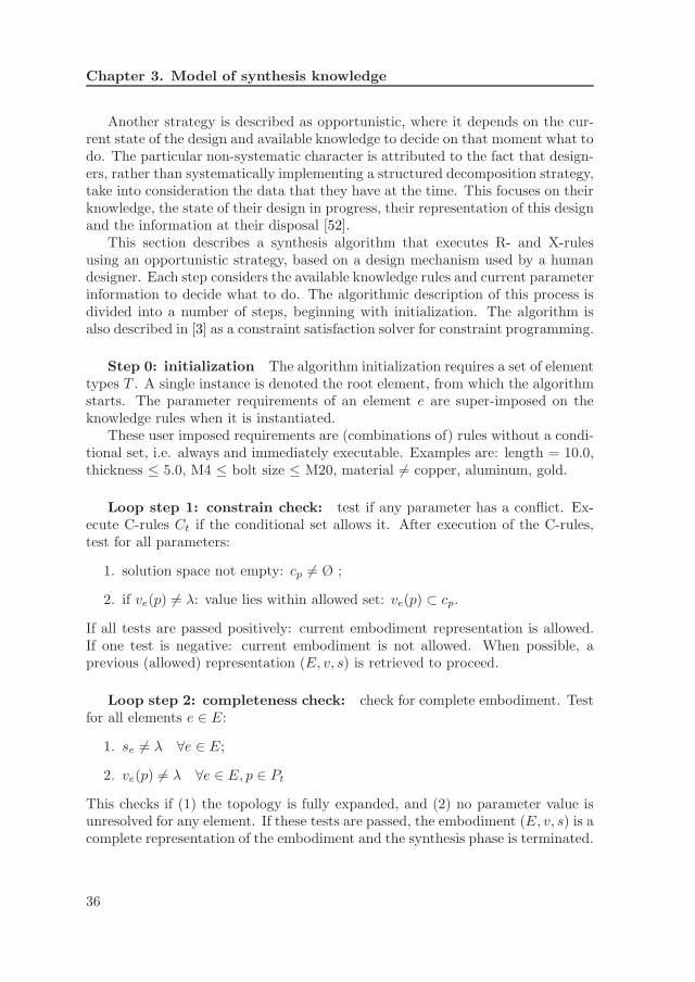
Chapter 3. Model of synthesis knowledge
Another strategy is described as opportunistic, where it depends on the cur-rent state of the design and available knowledge to decide on that moment what todo. The particular non-systematic character is attributed to the fact that design-ers, rather than systematically implementing a structured decomposition strategy,take into consideration the data that they have at the time. This focuses on theirknowledge, the state of their design in progress, their representation of this designand the information at their disposal [52].
This section describes a synthesis algorithm that executes R- and X-rulesusing an opportunistic strategy, based on a design mechanism used by a humandesigner. Each step considers the available knowledge rules and current parameterinformation to decide what to do. The algorithmic description of this process isdivided into a number of steps, beginning with initialization. The algorithm isalso described in [3] as a constraint satisfaction solver for constraint programming.
Step 0: initialization The algorithm initialization requires a set of elementtypes T . A single instance is denoted the root element, from which the algorithmstarts. The parameter requirements of an element e are super-imposed on theknowledge rules when it is instantiated.
These user imposed requirements are (combinations of) rules without a condi-tional set, i.e. always and immediately executable. Examples are: length = 10.0,thickness ≤ 5.0, M4 ≤ bolt size ≤ M20, material 6= copper, aluminum, gold.
Loop step 1: constrain check: test if any parameter has a conflict. Ex-ecute C-rules Ct if the conditional set allows it. After execution of the C-rules,test for all parameters:
1. solution space not empty: cp 6= Ø ;
2. if ve(p) 6= λ: value lies within allowed set: ve(p) ⊂ cp.
If all tests are passed positively: current embodiment representation is allowed.If one test is negative: current embodiment is not allowed. When possible, aprevious (allowed) representation (E, v, s) is retrieved to proceed.
Loop step 2: completeness check: check for complete embodiment. Testfor all elements e ∈ E:
1. se 6= λ ∀e ∈ E;
2. ve(p) 6= λ ∀e ∈ E, p ∈ Pt
This checks if (1) the topology is fully expanded, and (2) no parameter value isunresolved for any element. If these tests are passed, the embodiment (E, v, s) is acomplete representation of the embodiment and the synthesis phase is terminated.
36

3.5 Limitations
Loop step 3: advance partial embodiment: execute one R- or X-rule.This is done in three phases:
1. explore possibilities;
2. select parameter or element;
3. execute rule.
The first step tests the conditional sets for the R- and X-rules of each parameterand element, and gathers the possibilities. Second, one parameter or element isselected to be resolved or expanded. Using the concept of belief, a difference ismade between rules with and without random generation: rules without randomgeneration have a higher belief (equations before guesses). Selecting which pa-rameter or element to be resolved can be made with or without a strategy. In themost basic form, this is a random process.
As the third step, the action of the selected rule is executed, after which thealgorithm continues with loop step 1: constrain check.
Note 1: if backtracking to previous partial embodiments is implemented tosolve C-rule violations, the algorithm effectively implements a non-deterministicversion of depth-first search.
Note 2: no effort is taken to trace the origin of a conflict, because this can beseveral R-rules back inside a different element. Given the diversity of parameterand knowledge rules, as well as the “random walk” of the algorithm, this topic isreserved for future work.
3.5 Limitations
The PaRC model and the algorithm from Section 3.4 are used to automate syn-thesis of parametric engineering design, with the following limitations.
3.5.1 Systems of equations
The algorithm does not solve systems of equations. Developing a generic (au-tonomous) solver for a mix of linear, non-linear, logic relations for continuous anddiscontinuous parameters is outside scope of this thesis. However, the presence ofa system of equations is recognized by observing if a parameter can be resolved bymore than one R-rule. This signals that a system is encountered, and the currentembodiment is possibly incorrect and therefore abandoned. An example of thisapproach is given.
37

Chapter 3. Model of synthesis knowledge
Consider Equations (3.12) and (3.13) with two free parameters p1 and p2.
p1 + p2 = 2 (3.12)
p1· p2 = 1 (3.13)
These equations must be solved as a system in order to yield the only valid solutionp1 = 1 and p2 = 1. However, the nature of the algorithm is that it resolves oneparameter at a time. At the initial state, neither parameter can be resolved.The algorithm will randomly generate a value for one of the two parameters:e.g. p1 = 0.5. Next, the algorithm will explore the possibilities, and finds it canresolve p2 by R-rules derived from either (3.12) or (3.13). This leads to p2 = 1.5or p2 = 2, both incorrect.
The erroneous situation is prevented by observing the fact that p2 can beresolved by more than one R-rule (excluding random generation). If such a situ-ation is encountered, the entire embodiment is abandoned (the “better safe thansorry” paradigm is applied). A remedy for this situation is to add an additionalR-rule that recognizes specific systems of equations and solves them explicitly.
If one requires the algorithm to prevent systems of equations, one must state allparameters of an equation as possible resolve options. Even if no computationalmethod is included to actually resolve the parameter. This is done because theycould be part of a system, and this situation must be noticed.
3.5.2 Consistency and solvability
The consistency and/or solvability of a PaRC model is not explicitly checked.Therefore, it is possible to model ambiguous or erroneous situations and run thealgorithm. The algorithm will try to generate embodiments with the given model.
Autonomous analysis of the PaRC model would require the content of therules to meet some prescribed (formal) expressiveness. An algorithm would beexecuted to detect an over-constrained situation or the lack of any solution. Bothchecks would be valuable to execute during the knowledge engineering phase, butare outside scope of this thesis.
The algorithm from Section 3.4 only detects systems of equations (an over-constrained problem), but does not solve them. The existence of solutions ischecked by running the algorithm and waiting for a solution.
3.5.3 Revising decisions
The model does not allow revision of earlier made decisions. Parameter valuesthat have been resolved cannot be changed. Neither can sub-elements be expandedtwice. The reason is that a parameter value could influence decisions made later onduring synthesis. To prevent the risk of a loop, the action of resolving or expansion
38
3.5 Limitations
twice is not allowed. Instead, an “estimation” parameter can be introduced toestimate a first value, after which another parameter describes the final value.
The consequence of “forward only” generation is also that the topology isstatic: after sub-elements are added to an element, no modifications are made.The random-walk during synthesis creates differences in the topology, but in-formed adjustments are not made.
Adjusting an embodiment to better meet performance criteria is outside thescope of this thesis. Recommendations concerning this topic are made in Section7.2.
3.5.4 Algorithm
The disadvantages of the backtracking algorithm are known [3]. The risk of re-peated failure due to the same reason and the lack of memory for conflicting valuesof parameters are among the main risks of inefficiency. The fact that conflicts arenot detected before they really occurs is another disadvantage. However, its ro-bustness and the fact it is independent (to certain extent) of the content of therules make it an attractive baseline algorithm.
39

Chapter 4Knowledge engineering
method
This chapter describes a method to decompose and model a design process andthe knowledge in terms of PaRC. The method begins with a design process andone or more knowledge sources. Modeling a design process requires identifica-tion and typing of information entities, sub-processes and knowledge rules withnomenclature from the original source.
The method aims to aid the “what to look for and how to get it”-aspect ofknowledge acquisition. In case of a human source, the knowledge engineer acts asfacilitator to make the expert’s knowledge explicit.
The first step divides a design process into levels of abstraction. After asuitable level is selected for further modeling, the analysis method is formalizedand used to identify the embodiment and scenario. Subsequent formalization ofthe synthesis knowledge leads to a completed PaRC model.
The outline of the method is depicted in Figure 4.1. The individual steps areelaborated in the following sections.
41

Chapter 4. Knowledge engineering method
Identify levels of abstraction
Selection
Analysis formalization
Synthesis formalization
design process
processes / information,
divided in levels of abstraction
1 level of abstraction
embodiment and scenario
PaRC model
1.
2.
3.
4.
Figure 4.1: knowledge engineering
42

4.1 Step 1: identify levels of abstraction
4.1 Step 1: identify levels of abstraction
The first step to find the levels of abstraction is the identification of the perfor-mance parameters. Levels of abstraction emerge as performance parameters ofequal importance.
The performance parameters are found by asking an expert to describe thequality of a design, or what parameters decide the quality? Give a design to anexpert and ask how “good” it is: what aspects does he/she consider? Give twodifferent designs to an expert, and ask which design is the better one: again, whataspects are considered? What information decides if a design is not approved?
These questions are asked at several moments during the design process. Thegoal is to obtain a list of performance identifiers. Examples are cost, weight, max-imum stress, optimal speed, first eigenfrequency, dynamic response and stability.
After the performance parameters are known, identify levels of abstractionby grouping the performance indicators of equal importance and their analysismethods. Performances of higher importance are identified early on in the designprocess: on higher levels of abstraction. Performances of equal importance belongin the same level. When multiple levels exists, rank these relatively to each other.To complete the division of a design process into distinct levels of abstraction,state what the input and output information is for each level.
4.2 Step 2: selection
It is possible that the design process is traced from first conceptual design allthe way to detailed design for manufacturing. Many levels of abstraction areidentified, some of which are not suitable for modeling with PaRC. This stepselects the parts that are suitable, using the following check:
1. the analysis methods are known;
2. the degrees of freedom are known and a knowledge source is available (i.e.the problem is well-structured);
3. the design process can be described with parametric information and quan-tifiable data.
It is advisable to select entire levels of abstraction to maintain coherence ofthe decision making process. If a group of performance parameters is taken intoaccount to make a decision, these parameters should be of equal importance andprovide a complete image of the quality of a design.
43

Chapter 4. Knowledge engineering method
4.3 Step 3: analysis formalization
A design process is selected for further formalization. The current step involves theformalization of the analysis methods that quantify the performance parameters.This is done by asking “how” these performance parameters are calculated: theanalysis method.
If an explicit method is used, describe the input and output information asparametrically as possible. After all parameters are identified, begin typing eachas embodiment, scenario, auxiliary or performance. To decide which type a pa-rameter is, the following decision scheme is suggested:
1. embodiment: parameters and/or topological structures that a designer isallowed to manipulate;
2. scenario: description of a usage situation, often prescribed by external par-ties or a previous level of abstraction. A designer is not allowed to freelymanipulate these parameters;
3. auxiliary: can be substituted by either only scenario, or only embodiment.Auxiliary parameters are the dependent parameters, while embodiment andscenario are independent;
4. performance: calculated by a combination of embodiment and scenario.
This decision scheme is intended as a guideline. It should always be used incombination with the intended common sense understanding of embodiment, sce-nario and performance: an embodiment is the designed artifact or system, andscenarios are imposed from “outside”. Performance comes from combining anembodiment and scenario, and states something about the quality of a design.Auxiliary parameters are used to rewrite other parameters, or give some addi-tional information. These can be substituted without changing the “core” of thedesign process.
After all parameter have been typed, the embodiment descriptions from mul-tiple analysis methods are combined to give a complete embodiment on a singlelayer of abstraction.
It is not obliged to “keep” all parameters, as some can be eliminated by sub-stitution. All embodiment and scenario parameters are kept and only the majorauxiliary parameters. Including more or less parameters creates a trade-off be-tween the expressiveness of the model and the (computational) complexity.
Analysis methods occur in a number of different ways. Section 4.3.1 discussesseveral differences between simulation, formula and tacit analysis methods andhow to cope with them during decomposition.
Note: during the identification process of these parameters, be careful notto focus too much on a single exercise: an embodiment requirement (e.g. length= 10) can be mistaken for a scenario parameter. Vice versa, a scenario can be
44
4.3 Step 3: analysis formalization
mistaken for a degree of freedom: how much load can this bridge take? Whenmodeling a design process by focusing on a single exercise, there is the risk ofextrapolating the exercise to the entire process. During one exercise, an expertis likely to organize his/her activities in such a way that the expected difficultiesare addressed properly. However, the next exercise might have other difficulties,making the expert change him/her strategy. And the next exercise could changeagain.
4.3.1 Differences in analysis methods
As discussed previously, an analysis method calculates a performance parameterbased on an embodiment and scenario. Three common types of analysis methodsare discussed in this section.
Simulation
Simulations are used to reveal performance issues that are hard, or impossible,to quantify analytically. Finite element analysis is a popular example of suchsimulations, such as the crank shaft depicted in Figure 1.2a.
Before a simulation is executed, the embodiment model has to be defined.This can be an abstracted representation, such as two-dimensional wire framemodel to represent a bridge, or a detailed three-dimensional model of the samebridge. The scenario can be a static or dynamic load case: a frequency sweep toreveal eigenfrequencies, or simply gravity to see if a structure fails under its ownweight.
The crank shaft of Figure 1.2a shows a simulation of the material stressesunder mechanical and thermal load. Whatever embodiment the designers comeup with, these are analyzed under the same load and temperature scenario.
The model of the crank shaft is in this example the embodiment and the loadand temperature the scenario. All of these parameters have to be specified beforea simulation is ran to reveal the material stresses. An analysis simulation cannotbe inverted to determine an embodiment parameter.
Formula
Formulas can occur in parametric design problems during all sub-processes. Afterthe performance parameters have been identified, their means of quantificationare the analysis methods, which have the general layout of Equation (4.1).
< performance >= f(embodiment, scenario) (4.1)
For instance, the design of a spring element. The design goal is to exhibit aspecific force upon a fixed displacement, using Equation (4.2) to calculate force
45
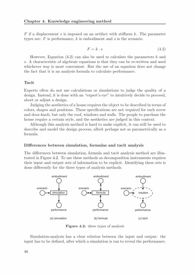
Chapter 4. Knowledge engineering method
F if a displacement s is imposed on an artifact with stiffness k. The parametertypes are: F is performance, k is embodiment and s is the scenario.
F = k · s (4.2)
However, Equation (4.2) can also be used to calculate the parameters k ands. A characteristic of algebraic equations is that they can be re-written and usedwhichever way is most convenient. But the use of an equation does not changethe fact that it is an analysis formula to calculate performance.
Tacit
Experts often do not use calculations or simulations to judge the quality of adesign. Instead, it is done with an “expert’s eye” to intuitively decide to proceed,abort or adjust a design.
Judging the aesthetics of a house requires the object to be described in terms ofcolors, shapes and positions. These specifications are not required for each screwand door-knob, but only the roof, windows and walls. The people to purchase thehouse require a certain style, and the aesthetics are judged in this context.
Although this analysis method is hard to make explicit, it can still be used todescribe and model the design process, albeit perhaps not as parametrically as aformula.
Differences between simulation, formulas and tacit analysis
The differences between simulation, formula and tacit analysis method are illus-trated in Figure 4.2. To use these methods as decomposition instruments requirestheir input and output sets of information to be explicit. Identifying these sets isdone differently for the three types of analysis methods.
embodiment
scenario
performance
simulation
embodiment
scenario
performance
formula
embodiment
scenario
performance
intuition
(a) simulation (b) formula (c) tacit
Figure 4.2: three types of analysis
Simulation-analysis has a clear relation between the input and output: theinput has to be defined, after which a simulation is ran to reveal the performance.
46

4.4 Step 4: synthesis formalization
This is used directly to distinct between the performance information and scenarioand embodiment information.
Formulas are explicit input-output relations, with the added difficulty thatformulas can be re-written algebraically, so what is the input and what is the out-put? For example, Equation (4.3) can be written as (4.4), (4.5) and (4.6). Fromobservation of the equations, it is not clear which one is the analysis expressionthat is needed for analysis-oriented decomposition.
The analysis expression is the one which is an explicit description of a per-formance parameter (see Expression (4.1)). The left-hand side states the perfor-mance and the right-hand side contains the scenario and embodiment. It dependson the design context which performance is relevant and which expression is theappropriate analysis formula.
p1 + p2 + p3 = 0 (4.3)
p1 = −p2 − p3 (4.4)
p2 = −p1 − p3 (4.5)
p3 = −p1 − p2 (4.6)
Tacit analysis methods lack explicit input-output relations. However, the in-formation can be divided into the three types. Once the performance informationis known, one asks “how” this is determined. The answer from the expert containsthe scenario and embodiment information. Similar to formulas, the goal is to ob-tain a description of “performance is determined by . . . ”, where the right-handside contains scenario and embodiment information.
4.4 Step 4: synthesis formalization
This phase uses the previously found parameters of the embodiment to acquireand model the knowledge rules for synthesis. The embodiment parameters arethe starting points to state the R-, C-rules and finally the elements and X-rules.
If the knowledge source mentions other parameters during knowledge acqui-sition, these can be added to the group and included in the acquisition process.Each parameter is made explicit with a name, short description and type (em-bodiment, scenario, performance or auxiliary), such as stated in Table 4.1. Thetable contains part of the embodiment of an industrial design case, discussed inmore detail in Section 6.2.1
47

Chapter 4. Knowledge engineering method
Table 4.1: optical chamber, parameters (partial)
type name description
scenario Smat sample materialTA tube surface areaTmat tube materialDetA detector surface area
embodiment Tx tube position, xTy tube position, yDmat diaphragm material... ...
auxiliary OCβP angle primary axisOCLP length primary axisEmax maximum energy... ...
The knowledge acquisition activity is one where questions are asked and an-swers formulated. The questions should lead to useful answers. The followingsection provides more detail how to acquire the relevant knowledge.
R-rule To obtain the R-rules for an object, specific answers are searched for:the condition statement and the action procedure (discussed in Section 3.3.3).
The general form of a R-rule for a parameter is:
if( <condition> )
{
<parameter value> = <action>
}
The condition and action statements are acquired by formulating an explicitanswer to the following questions:
1. condition: when can you calculate a value for this parameter?
2. action: how do you calculate the parameter value?
Example Expression (4.7) shows the action part of the R-rule to calculatethe x-coordinate of the tube (embodiment parameter Tx), Figure 4.3.
The action part of the R-rule to choose a diaphragm material is given inExpression (4.8). This rule selects material A if the value for Emax exceeds valueV, else material B is selected.
48
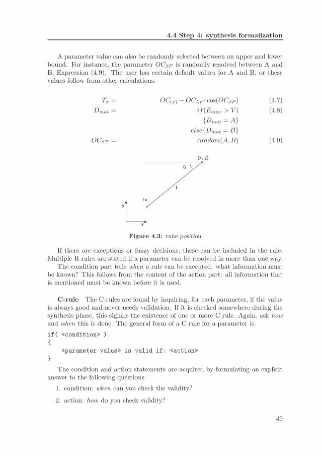
4.4 Step 4: synthesis formalization
A parameter value can also be randomly selected between an upper and lowerbound. For instance, the parameter OCβP is randomly resolved between A andB, Expression (4.9). The user has certain default values for A and B, or thesevalues follow from other calculations.
Tx = OC(x) − OCLP · cos(OCβP ) (4.7)
Dmat = if(Emax > V ) (4.8)
{Dmat = A}else{Dmat = B}
OCβP = random(A, B) (4.9)
L
ß
(x, y)
Tx
x
y
Figure 4.3: tube position
If there are exceptions or fuzzy decisions, these can be included in the rule.Multiple R-rules are stated if a parameter can be resolved in more than one way.
The condition part tells when a rule can be executed: what information mustbe known? This follows from the content of the action part: all information thatis mentioned must be known before it is used.
C-rule The C-rules are found by inquiring, for each parameter, if the valueis always good and never needs validation. If it is checked somewhere during thesynthesis phase, this signals the existence of one or more C-rule. Again, ask howand when this is done. The general form of a C-rule for a parameter is:
if( <condition> )
{
<parameter value> is valid if: <action>
}
The condition and action statements are acquired by formulating an explicitanswer to the following questions:
1. condition: when can you check the validity?
2. action: how do you check validity?
49

Chapter 4. Knowledge engineering method
Example An example of a C-rule is the check if a value exceeds a certainminimum ratio: Expression (4.10) must be valid. This yields the action parts ofC-rules (4.10),(4.11) and (4.12), for parameters a, b and c respectively. Eitherone of these three C-rules is sufficient to detect invalid embodiments, but forcompleteness all three are stated.
a ≥ b
c(4.10)
b ≤ a · c (4.11)
c ≥ b
a(4.12)
An example of a non-algebraic C-rule for parameter “material” is when certainmaterials are excluded for specific environments. The condition of the C-rule istrue if the environment is known. The action part will exclude all materials froma database that are sensitive to corrosion. The materials have a boolean to signalif they belong to the allowed set and this boolean can be made “false” by theC-rule, for example as shown in the following pseudo-code:
\\ CONDITION
if(E1.GetParameter(environment).IsResolved)
{
\\ rule can be executed
belief = 1.0
}
\\ ACTION
if(E1.GetParameter(environment).Value == corrosive)
{
\\ exclude sensitive materials
foreach(material in database)
{
if(material.CorrosionSensitive)
{
material.IsAllowed == false
}
}
}
Element types Element types are groups of parameters that are addressedsimultaneously. The question at this point is: what parameters belong together?
The product that is being design can be used to determine the element typesas physical entities, such as springs, belt drives, x-ray tube and detector.
Element types can also be defined according to different functions they performin a design. For example, an optical chamber (Section 6.2.1) has two diaphragm
50

4.4 Step 4: synthesis formalization
sets: one between tube and sample, and the other between sample and detector.Both sides have different functions and are modeled as different element types.The tube side must radiate the sample surface homogeneously, while the detec-tor side must focus on the center part of the sample. Both sides position theirdiaphragms differently. Instances of the element type “diaphragm” will occur assub-elements on both the tube and detector side.
The Vanderlande Industries case (Section 6.2.2) has element types specificallyto model product functions such as check-in, screening and sorting. Each of thesemain functions is a different element type, and within the main function areelement types for specific sub-functions, Figure 4.4. For example, the functionto gather incoming baggage flows, to redistribute the flow and make it evenlydistributed, to feed baggage in and out of the processing equipment and to presentit to the following sub-system. The element “belt” is used inside each functionalelement, but connected differently each time. Different element types are madefor different functions, and each function places its belts with specific knowledge.
Main function
Gather input Redistribute Process Output
Belt Belt Belt Belt BeltEq.
Figure 4.4: element types for functions
X-rule X-rules are revealed as the process that is executed to expand thetopology of the embodiment with new elements. Once the element types areidentified, the X-rules are formulated to add them.
An X-rule is executed when sufficient information is known to connect thesub-element(s) to existing parameters. After the expansion, each element will beself-supporting but must “know” its place within the topology. The layout of anX-rule is:
if ( <condition> )
{
\\ 1. create sub-element instances
\\ 2. connect to existing embodiment
\\ 3. add to element
}
The condition statement of the X-rule must check for the required informa-tion to connect the sub-elements to the embodiment. Formulation of the X-rulesdepends on the chosen element types.
51

Chapter 4. Knowledge engineering method
Note 1: knowledge rules can refer back to performance or scenario param-eters. For instance, a performance requirement is stated at the beginning andinfluences decisions during synthesis. If such parameters are mentioned duringsynthesis, these are included in the knowledge acquisition process.
Note 2: the parameters are revisited several times, to make sure no R- orC-rules are left out. Existing knowledge acquisition techniques are used to makethis process as efficient as possible.
Parameter dependency graph Synthesis knowledge is explicitly writtenas PaRC entities, but can also be graphically presented to visualize the parameterdependencies. Directed graphs are used to represent the network of parametersand R-rules. Parameter dependency graphs are used to observe more intuitively“what knowledge looks like”.
A parameter dependency graph consists of nodes and directed edges. Nodesrepresent parameters and the directed edges describe R-rules. The direction ofthe edges are pointed toward the target object: the parameter to resolve. If nodeD has N edges directed toward it, this represents a R-rule for node D that requiresthe N other values.
An example of such a parameter dependency graph is shown in Figure 4.5.This graph represents the R-rules derived from Equation 4.13, which comes froma compression spring. The equation describes the winding ratio w as a fractionof the spring diameter D and the wire diameter dwire.
w =D
dwire
(4.13)
Figure 4.5: parameter dependency graph, example
Node w has two edges directed toward it, meaning that its value can be re-solved if the values of D and dwire are known. As shown in Figure 4.5, theparameter value of dwire has no edges toward it. This means dwire cannot beresolved with this equation. The reason is that the allowed values of dwire are
52

4.5 The knowledge document
discontinuous (specified by a DIN standard), and a calculated value from an equa-tion is not guaranteed to be exactly a DIN value. Instead, dwire is resolved byanother rule, or random generator, before Equation 4.13 can be used to resolveeither w or D.
Note 1: The graphs are made using Graphviz win 2.16. The layout algo-rithm automatically aims edges in the same direction (top to bottom, or left toright) and then attempts to avoid edge crossings and reduce edge length (the so-called dot setting). Further analysis of these graphs is outside the scope of thisthesis: it is only intended as a graphical representation of knowledge.
Note 2: The random generation rule is not taken into account. Parametersthat do not occur in any R-rule are also not depicted.
4.5 The knowledge document
The result of the knowledge engineering phase is a model of the design processand synthesis knowledge that is described explicitly in a knowledge document.The model of the design process states the information flow through the differentsub-processes and the synthesis knowledge describes the knowledge is relevant forsynthesis. The latter is specified in PaRC entities of parameters, element types,X-, R- and C-rules.
The models within the knowledge document are not dependent of any singledesign exercise. The analysis method is used as guideline to determine the ex-pressiveness of the models, not the expert nor knowledge engineer. The goal is toretrieve a static, reliable model of the design process.
The document contains the knowledge as far as relevant to execute the designprocess and synthesis. No explanations, causal relationships or new knowledgeis included. However, these aspects can be added by using the PaRC model asstarting point and gathering more data.
The knowledge document contains valuable expert knowledge that can bestored or used for training purposes. However, the models can also be used todevelop design automation software. The following chapter will discuss the processof developing the software application.
4.6 Limitations
The knowledge engineering method is developed for engineering design with ex-isting knowledge, parametric information and quantitative data. Modeling theparameters and their R- and C-rules is relatively strictly prescribed. The modelcan be modified to the taste of the knowledge engineer, but a first model is madequite quickly. At least, that is the experience of the author.
53

Chapter 4. Knowledge engineering method
The scope further includes designs with topological degrees of freedom, such asassemblies and product systems. However, modeling topological entities requiresmore “personal creativity” of the knowledge engineer. These decisions are lessstrictly prescribed and therefor lead to more ad hoc modeling solutions. Althoughit is certainly possible to model designs such as transport networks, the goal ofthe method is to eliminate the ad hoc approach. The method is most suitable forparametric engineering with fewer topological degrees of freedom.
54
Chapter 5Software development
method
The development process of design automation software is prescribed for designcases that are unfamiliar to the development team. Guidelines are given aboutprocedure, as well as several approaches for efficient software development. Thepreviously described knowledge engineering method forms a substantial part ofthe process and is positioned relative to the other activities.
The software development process consists of steps depicted in Figure 5.1:the first step creates an overview of the major processes and products withinthe new company. Next, a section is selected for further study and model thedesign process using methods from Chapter 4. The PaRC model is subsequentlyautomated and the user interaction is determined.
The steps are described in more detail in the following sections. Divergingfrom this plan is of course allowed, but being aware of a procedure or informationstructure is a great benefit during software development, as concluded from thedevelopment of several prototypes [40].
55

Chapter 5. Software development method
Overview
Selection
Modeling (Chapter 4)
Automation
company
flowchart processes / products
1 design process
PaRC model
automatic synthesis
1.
2.
3.
4.
User interaction
design automation software
5.
Figure 5.1: software development
56
5.1 Step 1: overview
5.1 Step 1: overview
The first step is to create an overview of the company and check for suitabledesign processes, getting to know the unfamiliar design environment, individualsand nomenclature. This phase has no strict procedure, as it depends greatlyon the specific situation. The general goal is to create an overview of contextsurrounding the design of the product(s). Especially the input/output interfacesbetween departments, processes and activities are of interest.
A suggestion is to begin with a product family tree and process flowcharts frominitial requirements to final product specifications. State the activities and setsof information as they evolve from beginning to end. Where possible, specify thedesign processes with respect to e.g. disciplines (physics, mechanical), componentsor level of detail. Different departments and/or expert designers might embodyan isolated (part of a) process, as are chapters and sections in literature sources.
The output of this phase is an overview of the different (design) processes, rel-ative to each other. The information is specified in the company’s nomenclature.An overview can encompass multiple design processes and levels of abstractionfrom conceptual systems design to manufacturing planning.
5.2 Step 2: selection
Suitable design processes for software development are identified, using a suitabil-ity check that is similar to Section 4.2. In addition, the check here also takes intoaccount the ability to be automated. Design processes are required to meet thefollowing conditions:
1. the analysis methods automatically quantify a set of performance parame-ters;
2. (identical to Section 4.2) the degrees of freedom are known and a knowledgesource is available (i.e. the problem is well-structured);
3. (identical to Section 4.2) the design process can be described with paramet-ric information and quantifiable data.
5.3 Step 3: modeling
Developing a model of the selected design process and synthesis knowledge is doneusing the knowledge engineering method described in Chapter 4. First, levelsof abstraction within the design process are identified, and the most suitableone selected. The information around the analysis methods describes the coreexpressiveness of the software.
Once the parameters around the analysis method are made explicit, a modelof the design process is made. The content of the information sets of performance,
57
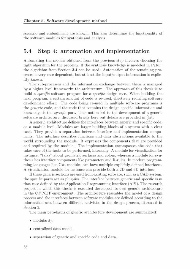
Chapter 5. Software development method
scenario and embodiment are known. This also determines the functionality ofthe software modules for synthesis and analysis.
5.4 Step 4: automation and implementation
Automating the models obtained from the previous step involves choosing theright algorithm for the problem. If the synthesis knowledge is modeled in PaRC,the algorithm from Section 3.4 can be used. Automation of the remaining pro-cesses is very case dependent, but at least the input/output information is explic-itly known.
The sub-processes and the information exchange between them is managedby a higher level framework: the architecture. The approach of this thesis is tobuild a specific software program for a specific design case. When building thenext program, a certain amount of code is re-used, effectively reducing softwaredevelopment effort. The code being re-used in multiple software programs isthe generic code, and the code that contains the design specific information andknowledge is the specific part. This notion led to the development of a genericsoftware architecture, discussed briefly here but details are provided in [48].
A generic architecture defines the interfaces between generic and specific code,on a module level. Modules are larger building blocks of a system with a cleartask. They provide a separation between interface and implementation compo-nents. The interface describes functions and data abstractions available to theworld surrounding the module. It expresses the components that are providedand required by the module. The implementation encompasses the code thattakes care of the tasks to be performed, internally. A module for visualization forinstance, “talks” about geometric surfaces and colors; whereas a module for syn-thesis has interface components like parameters and R-rules. In modern program-ming languages like C#, modules can have multiple explicitly defined interfaces.A visualization module for instance can provide both a 2D and 3D interface.
If these generic sections are used from existing software, such as a CAD system,the specific parts act as plug-ins. The interface between generic and specific is inthat case defined by the Application Programming Interface (API). The researchproject in which this thesis is executed developed its own generic architecturein the C#.NET environment. The architecture resembles the model of a designprocess and the interfaces between software modules are defined according to theinformation sets between different activities in the design process, discussed inSection 3.
The main paradigms of generic architecture development are summarized:� modularity;� centralized data model;� separation of generic and specific code and data.
58
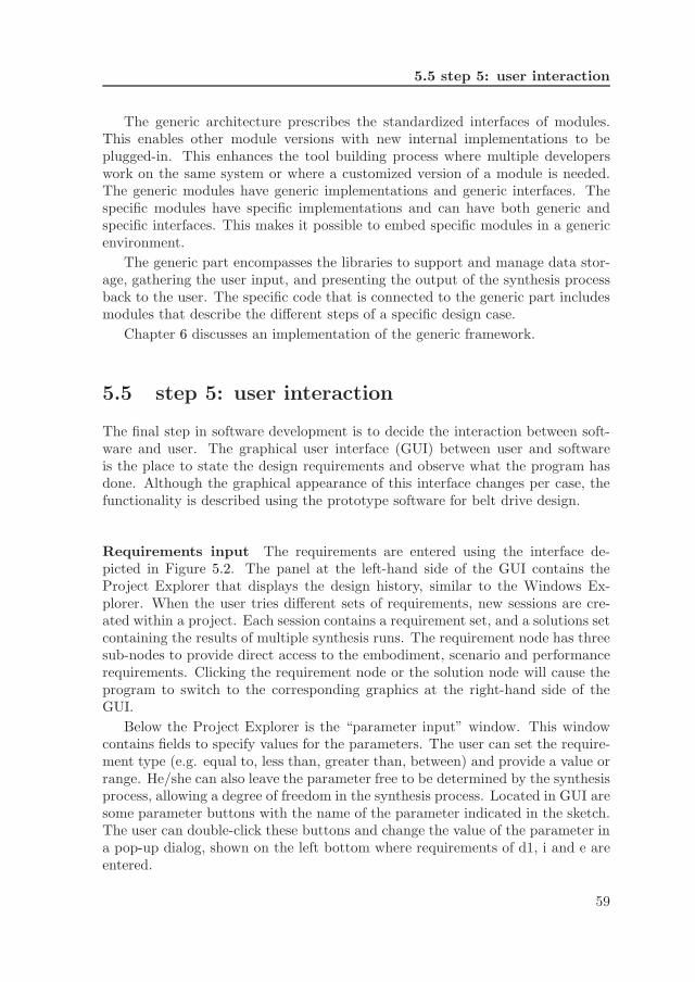
5.5 step 5: user interaction
The generic architecture prescribes the standardized interfaces of modules.This enables other module versions with new internal implementations to beplugged-in. This enhances the tool building process where multiple developerswork on the same system or where a customized version of a module is needed.The generic modules have generic implementations and generic interfaces. Thespecific modules have specific implementations and can have both generic andspecific interfaces. This makes it possible to embed specific modules in a genericenvironment.
The generic part encompasses the libraries to support and manage data stor-age, gathering the user input, and presenting the output of the synthesis processback to the user. The specific code that is connected to the generic part includesmodules that describe the different steps of a specific design case.
Chapter 6 discusses an implementation of the generic framework.
5.5 step 5: user interaction
The final step in software development is to decide the interaction between soft-ware and user. The graphical user interface (GUI) between user and softwareis the place to state the design requirements and observe what the program hasdone. Although the graphical appearance of this interface changes per case, thefunctionality is described using the prototype software for belt drive design.
Requirements input The requirements are entered using the interface de-picted in Figure 5.2. The panel at the left-hand side of the GUI contains theProject Explorer that displays the design history, similar to the Windows Ex-plorer. When the user tries different sets of requirements, new sessions are cre-ated within a project. Each session contains a requirement set, and a solutions setcontaining the results of multiple synthesis runs. The requirement node has threesub-nodes to provide direct access to the embodiment, scenario and performancerequirements. Clicking the requirement node or the solution node will cause theprogram to switch to the corresponding graphics at the right-hand side of theGUI.
Below the Project Explorer is the “parameter input” window. This windowcontains fields to specify values for the parameters. The user can set the require-ment type (e.g. equal to, less than, greater than, between) and provide a value orrange. He/she can also leave the parameter free to be determined by the synthesisprocess, allowing a degree of freedom in the synthesis process. Located in GUI aresome parameter buttons with the name of the parameter indicated in the sketch.The user can double-click these buttons and change the value of the parameter ina pop-up dialog, shown on the left bottom where requirements of d1, i and e areentered.
59

Chapter 5. Software development method
Figure 5.2: requirements input, belt drive case
60

5.5 step 5: user interaction
Solutions presentation In the Solutions view, the user is presented with thesolutions for a design problem, by means of a 2D plot or a list. A sketch of an in-dividual solution can be included at the right-hand side. A list of all embodimentsis visible and connected to the dots in the diagram. Each dot is an embodimentthat can be given a color. In this example, different colors represent different beltmaterials. Both diagram axes can handle all parameters, simply by selecting themfrom a drop-down box (currently it depicts “optimal belt speed” vs. “pre-load onaxis”).
Figure 5.3: solutions representation, belt drive case
61

Chapter 6Implementation and
realization
The knowledge engineering method of Chapter 4 and the software developmentmethod of Chapter 5 are applied to two groups of cases: tacit industrial andexplicitly documented.
Two tacit industrial cases are done in cooperation with two companies fromDutch industry. The first case discusses the software development for a productcomponent. The second case concerns the layout design of a transport network.Both cases did not have explicitly documented knowledge before hand.
The second group of cases are machine elements with explicitly documentedknowledge. Prototypes are developed to demonstrate PaRC for more familiardesigns.
The generic software framework as described in Section 5.4 is developed inC#.NET, with the functionality of the graphical user interface, synthesis andanalysis. The software architecture and several class diagrams are briefly discussedto shed some light on the implementation of the software. The prototypes aredeveloped using the generic framework.
6.1 Architecture
The software architecture is developed with the paradigms as discussed in Section5.4. The central data storage and separation of the synthesis and analysis moduleare the most visible properties of the architecture, depicted in Figure 6.1. Thecase specific software modules are the PaRC model, analysis module and somegraphics in the user interface.
The user interacts with the software through an input and output interface.The input module gathers the requirements and sends this to a central data
63
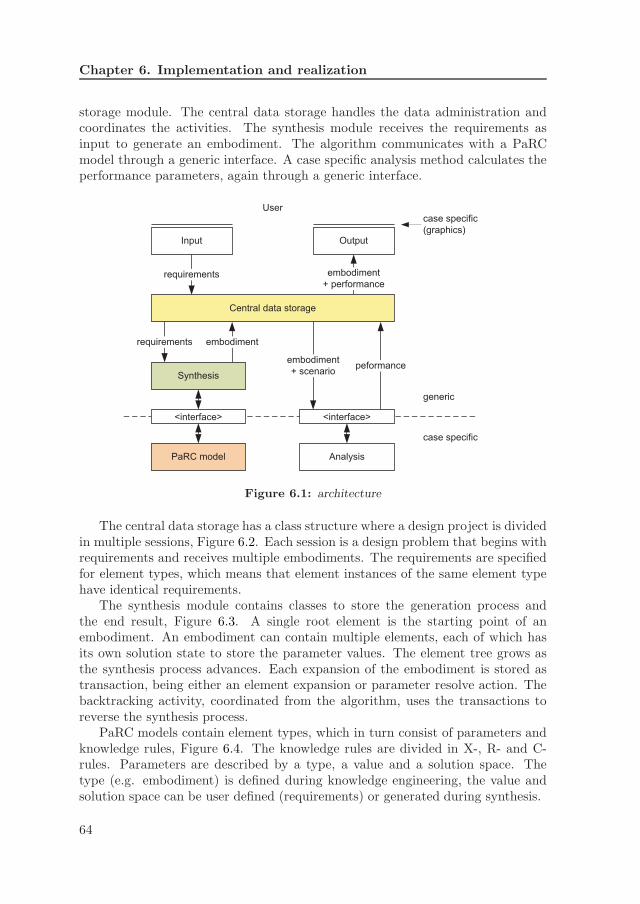
Chapter 6. Implementation and realization
storage module. The central data storage handles the data administration andcoordinates the activities. The synthesis module receives the requirements asinput to generate an embodiment. The algorithm communicates with a PaRCmodel through a generic interface. A case specific analysis method calculates theperformance parameters, again through a generic interface.
Input Output
Central data storage
Synthesis
PaRC model Analysis
requirements
requirements
embodiment
+ performance
embodiment
embodiment
+ scenariopeformance
<interface> <interface>
generic
case specific
Usercase specific
(graphics)
Figure 6.1: architecture
The central data storage has a class structure where a design project is dividedin multiple sessions, Figure 6.2. Each session is a design problem that begins withrequirements and receives multiple embodiments. The requirements are specifiedfor element types, which means that element instances of the same element typehave identical requirements.
The synthesis module contains classes to store the generation process andthe end result, Figure 6.3. A single root element is the starting point of anembodiment. An embodiment can contain multiple elements, each of which hasits own solution state to store the parameter values. The element tree grows asthe synthesis process advances. Each expansion of the embodiment is stored astransaction, being either an element expansion or parameter resolve action. Thebacktracking activity, coordinated from the algorithm, uses the transactions toreverse the synthesis process.
PaRC models contain element types, which in turn consist of parameters andknowledge rules, Figure 6.4. The knowledge rules are divided in X-, R- and C-rules. Parameters are described by a type, a value and a solution space. Thetype (e.g. embodiment) is defined during knowledge engineering, the value andsolution space can be user defined (requirements) or generated during synthesis.
64

6.1 Architecture
project session requirements
performance
1 1 1
n
1
1nelement type
n
Central data
storage
1
1
candidate
solution
1
1embodiment
1
scenario1
Figure 6.2: central data storage, class model
nSynthesis parameterelement
transactionparameter
resolved
element
expanded
<link>
<link>
1 1 1 1
1
1
1
n
n
1
1
1
1
solution stateroot elementn
Figure 6.3: synthesis module, class model
value
solution space
1 1
1
type
1
element type1 n
parameter
X-rule
R-rule
C-rule
n
n
n
PaRC modeln1
Figure 6.4: PaRC model, class model
65

Chapter 6. Implementation and realization
An implementation example of a knowledge base is given in Figure 6.5. Thecode illustrates how an element type (in this case the OpticalChamber) is definedin terms of parameters and knowledge rules.
The complete implementation contains 100+ classes with derivatives and over-ridden methods. The generic software is constantly being modified to test newalgorithms. Detailed discussion of the class structures or activity diagrams isoutside scope of this thesis.
66
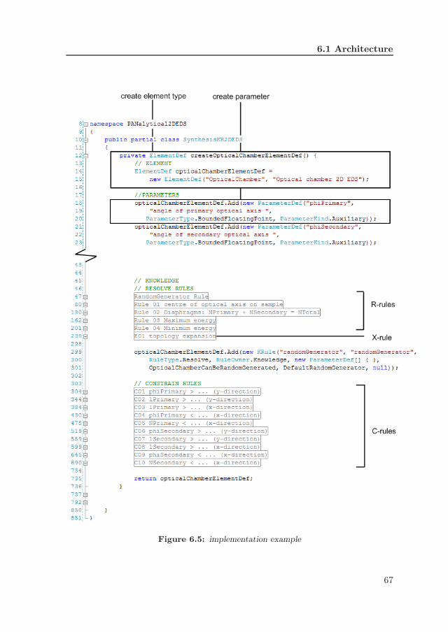
6.1 Architecture
Figure 6.5: implementation example
67
Chapter 6. Implementation and realization
6.2 Industrial cases
This section discusses two industrial cases: a product component and a networklayout.
6.2.1 Optical chamber of an XRF spectrometer
This case is done together with PANalytical and deals with the design of an opticalchamber of an x-ray spectrometer. The order of steps from Chapter 5 is followed.
Overview and selection
PANalytical is a high-tech company in The Netherlands that designs and manu-factures, among others, x-ray fluorescence spectrometers (Figure 6.6(a)). Theseinstruments are used to determine the chemical composition of materials. Theworking principle is that of x-ray fluorescence: high-energy x-ray is radiated ona sample material, causing element-characteristic photons to be expelled. Thesephotons are collected by a (solid state) energy dispersive detector and used todetermine the chemical composition of the sample, both qualitatively and quan-titatively. Wide applications in industry and research are a result of the abilityto analyze materials accurately and reproducibly.
The case focuses on the optical chamber of the so-called 2 Dimensional, EnergyDispersive X-Ray Fluorescence (2D EDS XRF) instrument. This case is chosenbecause of the well-known nature of the physics knowledge and the relative noveltyof the product range. A product tree with module specifications is made andrevealed that this type of optical chamber is exclusively designed for this type ofproduct.
Figure 6.6(a) shows the instrument with twelve cups in the carousel, each con-taining a different sample material. The measurement is executed by position-ing a cup above the optical chamber that radiates the sample from underneath.The main components of the optical chamber are schematically depicted in Fig-ure 6.6(b): the x-ray tube radiates the sample, causing fluorescence inside thematerial. This radiation enters the detector, after which digital data processingconstructs the chemical composition. Diaphragms are inserted to control the pathof the radiation, and an impenetrable casing encloses the components to shieldthe environment (and operator).
The components should be positioned in such a way that the tube radiatesthe sample brightly, and the detector “sees” only the radiated section of the sam-ple. Unfortunately, the diaphragms and casing cause unwanted fluorescence andreflections that also enter the detector and negatively influences the measurementquality.
68
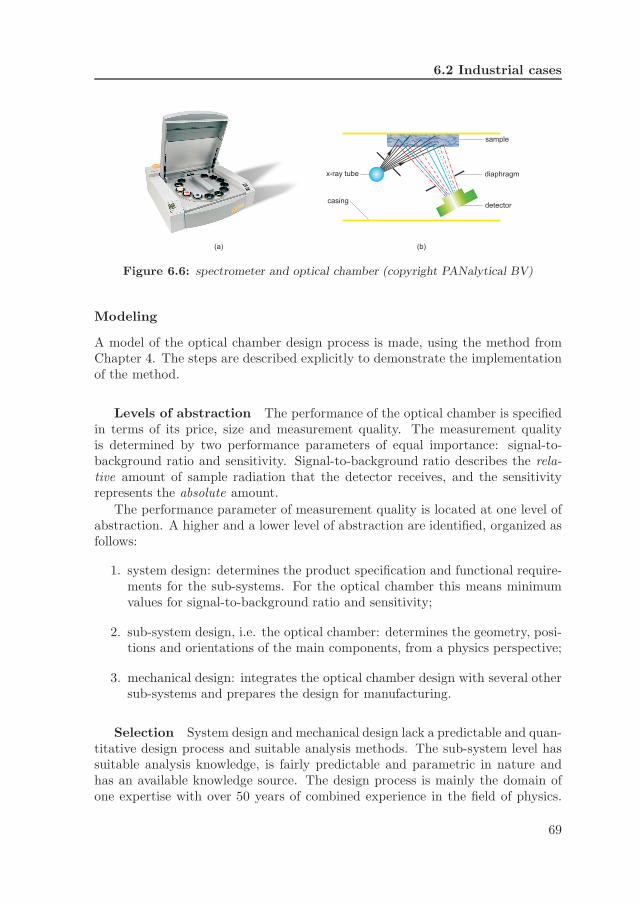
6.2 Industrial cases
sample
detector
diaphragmx-ray tube
casing
(a) (b)
Figure 6.6: spectrometer and optical chamber (copyright PANalytical BV)
Modeling
A model of the optical chamber design process is made, using the method fromChapter 4. The steps are described explicitly to demonstrate the implementationof the method.
Levels of abstraction The performance of the optical chamber is specifiedin terms of its price, size and measurement quality. The measurement qualityis determined by two performance parameters of equal importance: signal-to-background ratio and sensitivity. Signal-to-background ratio describes the rela-tive amount of sample radiation that the detector receives, and the sensitivityrepresents the absolute amount.
The performance parameter of measurement quality is located at one level ofabstraction. A higher and a lower level of abstraction are identified, organized asfollows:
1. system design: determines the product specification and functional require-ments for the sub-systems. For the optical chamber this means minimumvalues for signal-to-background ratio and sensitivity;
2. sub-system design, i.e. the optical chamber: determines the geometry, posi-tions and orientations of the main components, from a physics perspective;
3. mechanical design: integrates the optical chamber design with several othersub-systems and prepares the design for manufacturing.
Selection System design and mechanical design lack a predictable and quan-titative design process and suitable analysis methods. The sub-system level hassuitable analysis knowledge, is fairly predictable and parametric in nature andhas an available knowledge source. The design process is mainly the domain ofone expertise with over 50 years of combined experience in the field of physics.
69
Chapter 6. Implementation and realization
The design process consists, for a significant part, of trying new configurationsand improving these until the performance is satisfactory.
The design process of the optical chamber on sub-system level is selected forfurther modeling.
Analysis formalization As discussed previously, the relevant performanceof the optical chamber is mainly specified in terms of signal-to-background ratioand sensitivity.
The performance of a particular design is determined by an expert’s eye andseveral analytical estimations. Little simulation analysis is used during the designprocess, so the analysis method is a relatively tacit one. Ray tracing software isavailable, but the required calculation time makes this unsuitable to use duringthe early phases of the design process.
Studying the analysis method and discussion with the expert reveals two levelsof detail as far as physics is concerned. The dominant effects of absorption, reflec-tion and fluorescence are of primary importance, while energy shifts, polarizationand penetration depth are of secondary.
A finite element analysis method is developed based on these assumptions tosimulate an expert’s judgment of the quality of a design. The formalization (andautomation) of the analysis method leads to the identification of the embodi-ment parameters. The scenario is determined on the system level and contains 4parameters: sample material, the tube material and size and detector size.
Synthesis formalization The analysis method requires an embodimentmodel with the expressiveness depicted in Figure 6.7: 22 parameters describethe geometry, position and orientation of the components. Discussing the embod-iment with the expert, and how this is created, revealed 18 auxiliary parametersto capture the design intent of the x-ray application and several geometric con-struction parameters. The R- and C-rules are acquired for each embodimentparameter.
The parameters are grouped into 8 element types: optical chamber, tube,detector, sample, diaphragm and casing. In addition, there are two element typesthat represent the two diaphragm sets, one on either side of the sample. Thisis done because there is different knowledge for the positioning and design ofdiaphragms on either side. Only a single diaphragm is depicted, but multiplediaphragms can be inserted.
A full description of the synthesis knowledge is provided in Appendix A.1 andsummarized in Table 6.1. An example of a (simplified) X-rule is given in pseudocode. The rule adds a number of diaphragms to the primary set, on a randomx-coordinate between the tube and the sample. The diaphragms are placed fromleft to right, and (in this example) a C-rule checks if the diaphragms do notintersect.
70
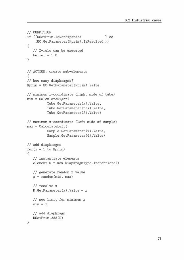
6.2 Industrial cases
// CONDITION
if ((DSetPrim.IsNotExpanded ) &&
(OC.GetParameter(Nprim).IsResolved ))
{
// X-rule can be executed
belief = 1.0
}
// ACTION: create sub-elements
{
// how many diaphragms?
Nprim = OC.GetParameter(Nprim).Value
// minimum x-coordinate (right side of tube)
min = CalculateRight(
Tube.GetParameter(x).Value,
Tube.GetParameter(phi).Value,
Tube.GetParameter(A).Value)
// maximum x-coordinate (left side of sample)
max = CalculateLeft(
Sample.GetParameter(x).Value,
Sample.GetParameter(d).Value)
// add diaphragms
for(i = 1 to Nprim)
{
// instantiate elements
element D = new DiaphragmType.Instantiate()
// generate random x value
x = random(min, max)
// resolve x
D.GetParameter(x).Value = x
// new limit for minimum x
min = x
// add diaphragm
DSetPrim.Add(D)
}
71
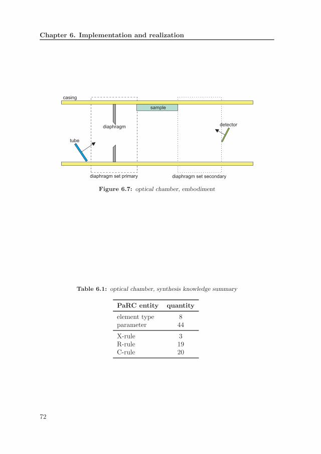
Chapter 6. Implementation and realization
tube
detectordiaphragm
sample
casing
diaphragm set primary diaphragm set secondary
Figure 6.7: optical chamber, embodiment
Table 6.1: optical chamber, synthesis knowledge summary
PaRC entity quantity
element type 8parameter 44
X-rule 3R-rule 19C-rule 20
72

6.2 Industrial cases
Figure 6.8 shows the parameter dependency graph of the synthesis knowledge.The labels in the nodes are formatted as Expression (6.1), using the elementnames from Table A.1 and parameter names in Table A.2.
< element name > < parameter name > (6.1)
Software development The user interface is shown in Figure 6.9. Theinsert window shows the required number of embodiments to be generated (200)and the mesh settings for analysis.
Figure 6.10 shows the output of the software and several customized analysisoutputs. The top left section displays a plot of the solution space, where eachdot is an embodiment (about 2.500 are generated). This particular plot showssignal-to-background plotted against sensitivity, but any combination of param-eters can be selected on the axes. The top right corner shows a sketch of theselected embodiment, with directly below it some detailed quantification of theperformance. Bottom row shows (right to left): an estimation of the spectrum,an estimation of the detector view (horizontal axis is the length of the detector),and a more detailed view of the background ratio (in this case revealing that thetube is by far the largest contributor).
Validation Validation of the software is done through expert evaluation.Several scenarios and parameter sensitivities are compared to expected valuesfrom experience.
The quality of the analysis module is validated as proportional to expectations.This means the software can be used to rank solutions according to calculatedperformances, which is in accordance with the intended use of a synthesis tool.
Validation of the generated solutions shows expected characteristics, althoughthe “shape” of the solution clouds (e.g. Figure 6.10) is sometimes surprising. Theexpert whose knowledge is implemented expects a significant reduction in designtime.
The knowledge document and the division of the design process into levels ofabstraction provide insight in the activities and decision moments. The informa-tion between levels is made explicit and aware to the relevant people. This helpsto prevent miscommunication and unnecessary iteration loops.
The explicit nature of the shape of the cloud serves as communication toolbetween disciplines. For experts from different domains, the trends and limitationsof solution cloud is helpful to discuss possibilities. Figure 6.11 shows the solutionsin a plot of a performance parameter versus an embodiment parameter. From thefigure, it is clear that a limit exist for the embodiment parameter to achieve acertain minimum performance. Experts from other disciplines see what it meanswhen they ask a 10% increase of an embodiment parameter.
73
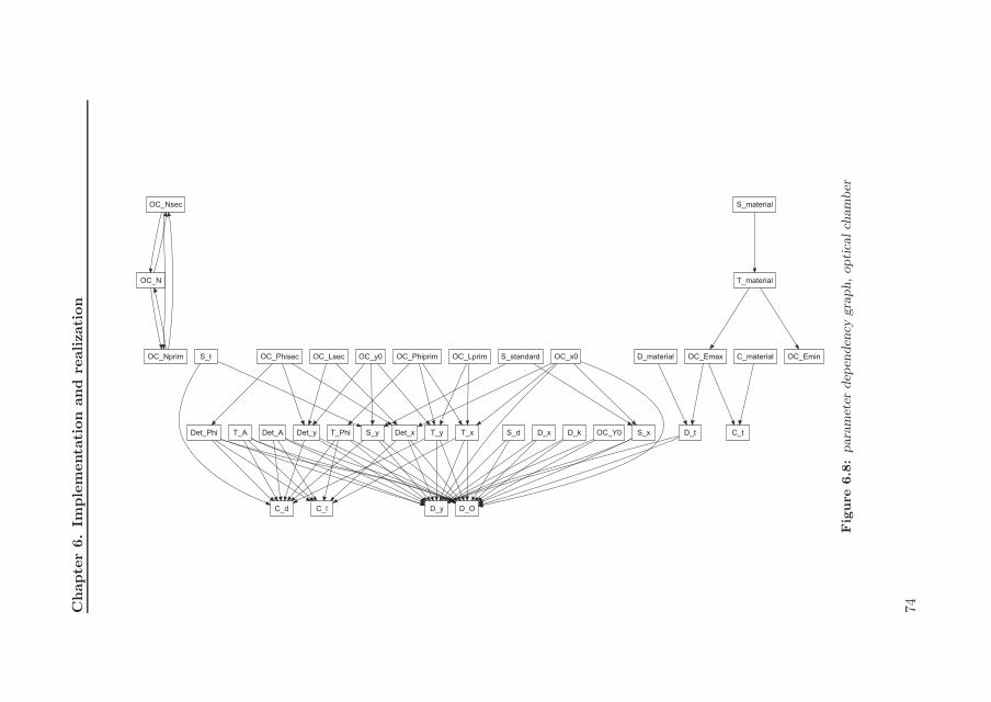
Chapte
r6.
Imple
menta
tion
and
realizati
on
OC_Nsec
OC_N
OC_Nprim
T_material
OC_Emax OC_Emin
C_tD_t
OC_x0
T_xDet_x S_x
D_OD_yC_l
OC_Lprim
T_y
OC_Phiprim
T_Phi
S_material
OC_y0
Det_y S_y
C_d
OC_LsecOC_Phisec
Det_Phi T_A Det_A
S_t C_materialS_standard
D_x D_k OC_Y0S_d
D_material
Fig
ure
6.8
:para
met
erdep
enden
cygra
ph,optica
lch
am
ber
74

6.2 Industrial cases
Figure 6.9: user interface, input
Figure 6.10: user interface, output
75
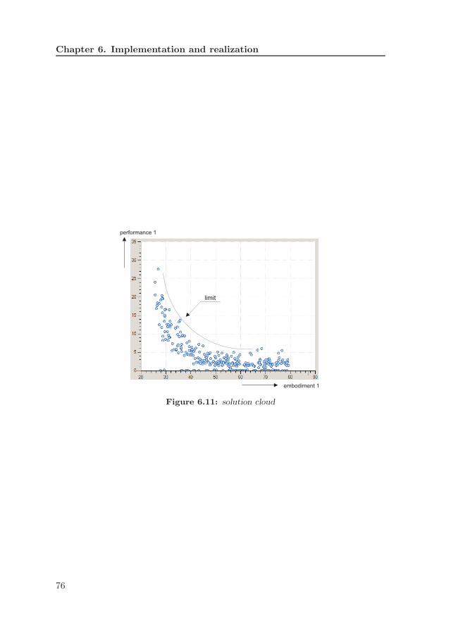
Chapter 6. Implementation and realization
performance 1
embodiment 1
limit
Figure 6.11: solution cloud
76

6.2 Industrial cases
6.2.2 Baggage handling system
A synthesis module is developed for the design of transport networks, in coop-eration with Vanderlande Industries. The topological freedom of such designsis modeled by introducing multiple levels of element types. The knowledge toexpand the topological tree is located inside the X-rules.
Overview Vanderlande Industries is a Dutch company that designs andmanufactures, among others, baggage handling systems (BHS). These multi-million dollar systems are found in larger airports to process the baggage througha series of belts, scanning devices and sorters toward the aircraft. A schematicview of such a BHS is shown in Figure 6.12.
Figure 6.12: baggage handling system (copyright Vanderlande Industries)
The BHS design process begins with an airport as customer and ends withtechnical drawings of all parts. The process is divided into three major levels ofabstraction:
1. process flow design (PFD): determines the functional design of a BHS, i.e.what process operations the system performs on a piece of baggage, suchas check-in, screening and sorting. A PFD design is shown in Figure 6.13.The design is determined in several discussions with the customer;
2. material flow design (MFD): translates the process flow design into a quanti-fied transport network. At this level there are about 20-30 distinct functionalpieces of equipment that constitute a BHS design;
3. detail design: specifies all mechanical and electronic equipment, ready forproduction.
77
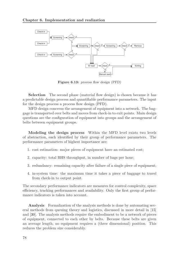
Chapter 6. Implementation and realization
Check-in
Screening
Screening Remove
ID read
Manual read
Sorting
check
check
Check-in
Check-in Screening
check check
check
Screening
n
y
n
y n
y
n
y
n
y
Figure 6.13: process flow design (PFD)
Selection The second phase (material flow design) is chosen because it hasa predictable design process and quantifiable performance parameters. The inputfor the design process a process flow design (PFD).
MFD design concerns the arrangement of equipment into a network. The bag-gage is transported over belts and moves from check-in to exit points. Main designquestions are the configuration of equipment into groups and the arrangement ofbelts between equipment groups.
Modeling the design process Within the MFD level exists two levelsof abstraction, each identified by their group of performance parameters. Theperformance parameters of highest importance are:
1. cost estimation: major pieces of equipment have an estimated cost;
2. capacity: total BHS throughput, in number of bags per hour;
3. redundancy: remaining capacity after failure of a single piece of equipment;
4. in-system time: the maximum time it takes a piece of baggage to travelfrom check-in to output point.
The secondary performance indicators are measures for control complexity, spaceefficiency, tracking performances and availability. Only the first group of perfor-mance indicators is taken into account.
Analysis Formalization of the analysis methods is done by automating sev-eral methods from queuing theory and logistics, discussed in more detail in [15]and [30]. The analysis methods require the embodiment to be a network of piecesof equipment, connected to each other by belts. Because these belts are givenan average length, no equipment requires a (three dimensional) position. Thisreduces the problem size considerably.
78

6.2 Industrial cases
The analysis methods led to the embodiment parameters and element types.The PFD processes are high level embodiment element types with a generic struc-ture: illustrated in Figure 6.14. Each PFD process expands with three sub-elements: belt network, equipment group set and baggage flow. The belt networkcollects the baggage flows from upstream PFD processes. It will construct a net-work of belts, merge and divert equipment to rearrange the baggage flow. Theequipment group contains the pieces of equipment that operate on the baggageflows, e.g. screening and sorting. The baggage flow at the right side of thePFD process is ready to be connected to a downstream PFD processes. Thisdownstream PFD process is instantiated once the current output baggage flow isresolved.
The network connections are made through ID tagging: each instantiatedelement has a parameter that is the ID of the element it is connected to. Theseparameters define an embodiment.
PFD process
belt network equipment group set baggage
flow
baggage
flow
belt belt
ne
two
rk
equipment group
equipment ...
...
...
...
equipment
baggage
flow
belt
...
Figure 6.14: PFD process
Synthesis Separating the knowledge of different PFD functions breaks thetotal design problem down into manageable chunks. These PFD functions havean identical structure except the check-in, sorting and baggage removal. Thesynthesis knowledge is given in Appendix A.2 and summarized in Table 6.2.
Table 6.2: BHS design, synthesis knowledge summary
PaRC entities quantity
element type 51parameter 204
X-rule 46R-rule 120C-rule 0
79
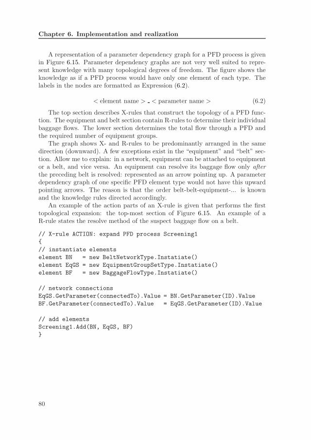
Chapter 6. Implementation and realization
A representation of a parameter dependency graph for a PFD process is givenin Figure 6.15. Parameter dependency graphs are not very well suited to repre-sent knowledge with many topological degrees of freedom. The figure shows theknowledge as if a PFD process would have only one element of each type. Thelabels in the nodes are formatted as Expression (6.2).
< element name > < parameter name > (6.2)
The top section describes X-rules that construct the topology of a PFD func-tion. The equipment and belt section contain R-rules to determine their individualbaggage flows. The lower section determines the total flow through a PFD andthe required number of equipment groups.
The graph shows X- and R-rules to be predominantly arranged in the samedirection (downward). A few exceptions exist in the “equipment” and “belt” sec-tion. Allow me to explain: in a network, equipment can be attached to equipmentor a belt, and vice versa. An equipment can resolve its baggage flow only afterthe preceding belt is resolved: represented as an arrow pointing up. A parameterdependency graph of one specific PFD element type would not have this upwardpointing arrows. The reason is that the order belt-belt-equipment-... is knownand the knowledge rules directed accordingly.
An example of the action parts of an X-rule is given that performs the firsttopological expansion: the top-most section of Figure 6.15. An example of aR-rule states the resolve method of the suspect baggage flow on a belt.
// X-rule ACTION: expand PFD process Screening1
{
// instantiate elements
element BN = new BeltNetworkType.Instatiate()
element EqGS = new EquipmentGroupSetType.Instatiate()
element BF = new BaggageFlowType.Instatiate()
// network connections
EqGS.GetParameter(connectedTo).Value = BN.GetParameter(ID).Value
BF.GetParameter(connectedTo).Value = EqGS.GetParameter(ID).Value
// add elements
Screening1.Add(BN, EqGS, BF)
}
80
6.2 Industrial cases
// R-rule ACTION: retrieve baggage flow of connected equipment
{
// get connected equipment, get flow
connectedTo = Belt.GetParameter(connectedTo).Value
suspect = GetElementByID(connectedTo).
GetParameter(suspect)
// resolve suspect flow
Belt.GetParameter(suspect).Value = suspect
}
Automation The synthesis module is automated to generate embodiments,based on a PFD design. In case of the PFD layout of Figure 6.13, the generatedembodiment is depicted in Figure 6.16. The analysis modules are not integrateddue to time constraints.
The feedback from industry is encouraging for further development of designautomation software to support the design on systems level.
81

Chapter 6. Implementation and realization
PFD_connectedToID
BeltNetwork_connectedToID EqGroupSet_connectedToID
BaggageFlow_connectedToID
Belt_connectedToID
EqGroup_connectedToID
Eq_suspect
Belt_suspect
Eq_cleared
Belt_cleared
Eq_IDread
Belt_IDread
Eq_IDNotRead
Belt_IDNotRead
PFD_numberofInputBelts
BaggageFlow_totalFlow
PFD_totalFlow
PFD_numberOfGroups
PFD_numberofOutputBelts
Eq_connectedToID
Belt_totalFlow
equipment
belt
expand network
total flow andnumber of input belts
Figure 6.15: parameter dependency graph, baggage handling system
82

6.2
Industria
lcase
s
PROCESS_2
PROCESS_3
PROCESS_4
PROCESS_5
PROCESS_6
PROCESS_7
PROCESS_8
PROCESS_9
PROCESS_10
PROCESS_11PROCESS_12
PROCESS_13
PROCESS_14
PROCESS_15
PROCESS_16
PROCESS_17
check-in screeninglevel 1
check+ split
screeninglevel 2
screeninglevel 3
check+ split
check +split
check+ split
bagremoval
ID read manualID read
sortation
beltnetwork
Fig
ure
6.1
6:
materia
lflow
dia
gra
m
83

Chapter 6. Implementation and realization
6.3 Explicitly documented cases
This section gives PaRC models of four machine elements: a flat belt drive and acompression, extension and torsion spring. The knowledge source is an engineer-ing handbook for design of machine elements [25].
The presented description of machine elements is not meant as the knowledgeof the element, rather as an example what a PaRC description could look like.The descriptions can be expanded or contracted by taking more parameters orrules into account, or ignoring others. Discussions about the optimal knowledgemodels of machine elements is outside the scope of this thesis.
6.3.1 Belt drive
A belt drive is a rotating transmission that features a pulling belt as power trans-mission element, Figure 6.17(a). Knowledge for belt drive design is documentedin eight pages [25], including theoretical principles, calculations and several prac-tical considerations for design. An example of how one analysis formula leads toother rules and parameters is given first.
One of the performance parameters is the stress σ within the belt. Quantifyingthis stress requires some geometric information plus a load scenario: Equation(6.3).
σ =F1
w· t (6.3)
With F1 being the force in the pulling part of the belt, and w and t the beltwidth and thickness, respectively. Following the literature, F1 is further specifiedas Equation (6.4).
F1 = Ft· k (6.4)
With Ft the force resulting from the applied torque T1 (6.5) and k being a usabilityfactor derived from embodiment parameters.
Ft =2·T1
d1(6.5)
The analysis Equation (6.3) leads to a number of parameters: σ, F1, Ft, T1, w,t, d1 and k. Deciding on the type of each parameter is done using the previouslydiscussed decision scheme, leading to:� embodiment: d1, w and t;� scenario: T1;� performance: σ, F1, Ft;� auxiliary: k.
84

6.3 Explicitly documented cases
Including F1 and Ft in the model increases the expressiveness but can alsobe discarded and substituted by other parameters. It depends on the goal of themodel (e.g. education, automation) which expressiveness is sufficient.
Figures 6.17(b) and (c) show the embodiment and scenario, respectively. Theparametric model of a belt drive is stated in Table 6.3.
d1 d2
t, w, material
e
n1
T1
P1
n2
T2
P2
(a) (b) (c)
Figure 6.17: belt drive, embodiment and scenario
Table 6.3: belt drive description
parameter type name description
performance Fa load on axesPeff effective power transmission
v belt speedσmax/σ safety factor on stress
fbmax/fb safety factor on bending
scenario T1 torque on pulley 1T2 torque on pulley 2n1 rotation speed of pulley 1n2 rotation speed of pulley 2P1 power on pulley 1P2 power on pulley 2
embodiment d1 diameter of driving pulleyd2 diameter of driven pulleye distance between axesw belt widtht belt thickness
material belt material
auxiliary i transmission ratiok usability characteristicm force ratioβ smallest enclosed arc
Continued on next page
85

Chapter 6. Implementation and realization
Table 6.3 – continued from previous page
parameter type name description
Ltotal length of constructionLbelt length of beltvopt optimal belt speed
R-rules The following equations are translated into R-rules, listed in Equa-tion Set (6.6). The right side indicates which parameters can be resolved throughthe equation.
i =d2
d1→i, d1, d2
i =n1
n2→i, n1, n2
i =T2
T1→i, T1, T2
P1 = n1·T1 →P1, n1, T1
P2 = n2·T2 →P2, n2, T2
P1 = P2 →P1, P2 (6.6)
Ltotal =d1
2+
d2
2+ e →Ltotal, d1, d2, e
m = eµ·β →m
k =m − 1
m→m, k
β = 2· cos−1
(
dlarge − dsmall
e
)
→β
Lbelt = 2· e· sin(
β
2
)
+π
2· (dlarge − dsmall)
+π
2·(
1 − β
π
)
· (dlarge − dsmall) →Lbelt, e
86

6.3 Explicitly documented cases
C-rules The C-rules from Equation Set (6.7) are included, in addition tothe default solution space for each parameter, such as d1 > 0.01, d1 < 0.5 and adatabase of 5 belt materials.
e ≥ d1
2+
d2
2→e, d1, d2
d1 ≥ w →d1, w
d2 ≥ w →d2, w
d1 ≥ t· fb →d1, t, material (6.7)
d2 ≥ t· fb →d2, t, material
w ≥ t →w, t
e ≥ 0.7· (d1 + d2) →e, d1, d2
e ≤ 2· (d1 + d2) →e, d1, d2
if(i ≥ 1) :e ≥ 0.9· d2 →e, d2
Where fb is the maximum bending ratio of belt material. The user interface forthe embodiment requirements is shown in Figure 6.19, together with the solutionsas a plot, list and one sketch. Figure 6.18 shows the parameter dependency graphof a belt drive. Table 6.4 summarizes the knowledge that is taking into accountduring synthesis.
Table 6.4: belt drive, synthesis knowledge summary
PaRC entity quantity
element type 1parameter 18
X-rule 0R-rule 27C-rule 23
87

Chapter 6. Implementation and realization
d1
d2
i
l
e
betaRad
beltLength
n1
n2
T1
T2
P1
P2
m
k
material
Figure 6.18: parameter dependency graph, belt drive
88
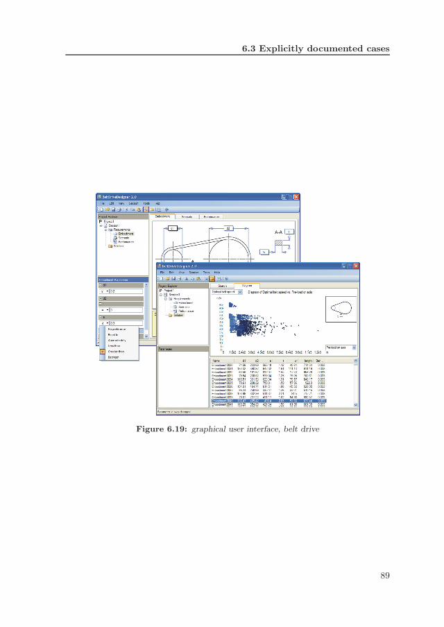
6.3 Explicitly documented cases
Figure 6.19: graphical user interface, belt drive
89

Chapter 6. Implementation and realization
6.3.2 Compression spring
Figure 6.20 shows the spring and the GUI of the synthesis tool. Table 6.5 sum-marizes its synthesis knowledge. A complete description is found in AppendixA.3.
Figure 6.20: compression spring
Table 6.5: compression spring, synthesis knowledge summary
PaRC entity quantity
element type 1parameter 24
X-rule 0R-rule 45C-rule 31
The parameter dependency graph of a compression spring is shown in Figure6.21.
90
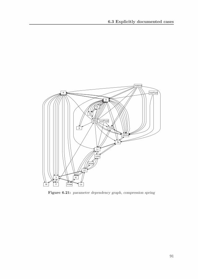
6.3 Explicitly documented cases
R
D
nActive
s
W F
sc
Fmax
Sa
De
w
Di
dWire
Lc
nTotal
material
L0
Ls
Lmin
smax
loadType
endFinish
Figure 6.21: parameter dependency graph, compression spring
91

Chapter 6. Implementation and realization
6.3.3 Extension spring
Figure 6.22 shows the extension spring and the GUI of the synthesis tool. Table 6.6summarizes its synthesis knowledge. A complete description is found in AppendixA.4.
Figure 6.22: extension spring
Table 6.6: extension spring, synthesis knowledge summary
PaRC entity quantity
element type 1parameter 24
X-rule 0R-rule 42C-rule 27
92
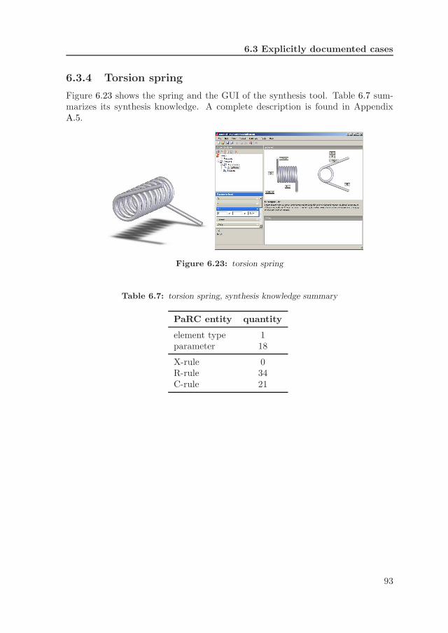
6.3 Explicitly documented cases
6.3.4 Torsion spring
Figure 6.23 shows the spring and the GUI of the synthesis tool. Table 6.7 sum-marizes its synthesis knowledge. A complete description is found in AppendixA.5.
Figure 6.23: torsion spring
Table 6.7: torsion spring, synthesis knowledge summary
PaRC entity quantity
element type 1parameter 18
X-rule 0R-rule 34C-rule 21
93

Chapter 6. Implementation and realization
6.4 Comparison
This section compares the models of synthesis knowledge of the previously dis-cussed cases, summarized in Table 6.8.
Table 6.8: synthesis knowledge, comparison
caseelementtypes parameters R-rules C-rules X-rules
belt drive 1 18 27 23 0compression spring 1 24 45 31 0extension spring 1 24 42 27 0torsion spring 1 18 34 21 0optical chamber 8 44 19 20 3baggage handl. sys. 51 204 120 0 46
6.4.1 R-rules
Figure 6.24 compares the amount of R-rules with the number of parameters. Thisindicates the amount of “deterministic” knowledge in relation to the size of theproblem. The figure depicts a dotted line that represents equal amounts of pa-rameters and R-rules. It shows that the industrial cases have fewer R-rules perparameter compared to the literature cases. The literature cases are located rela-tively close together, indicating similar amounts of knowledge for similar problemsizes. The cases of belt drive and the three springs have, on average, more thanone R-rule per parameter, a feature that is discussed with more detail next.
0
20
40
60
80
100
120
140
0 50 100 150 200
reso
lve
ru
les
parameters
industrial cases
literature cases
Figure 6.24: R-rules versus parameters
94
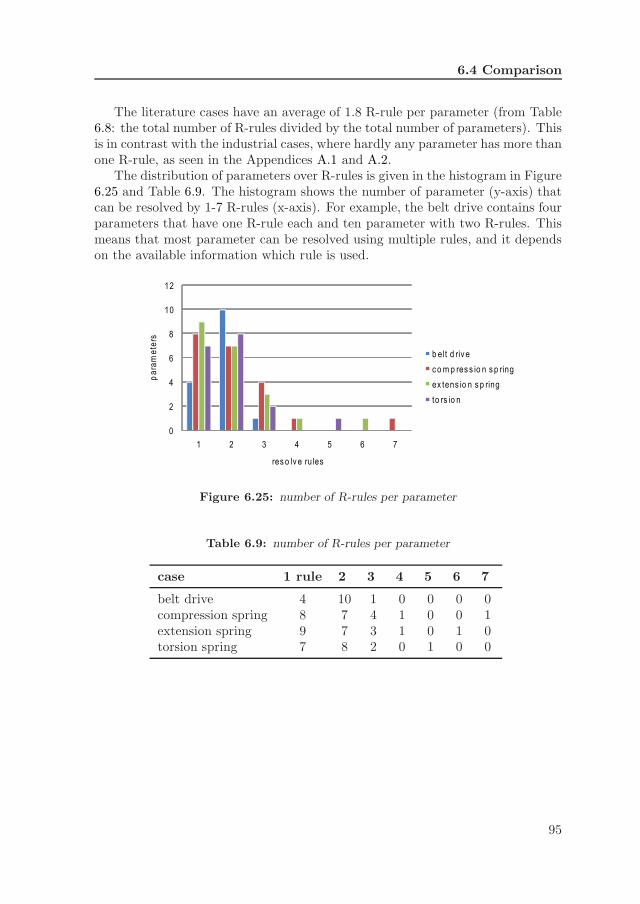
6.4 Comparison
The literature cases have an average of 1.8 R-rule per parameter (from Table6.8: the total number of R-rules divided by the total number of parameters). Thisis in contrast with the industrial cases, where hardly any parameter has more thanone R-rule, as seen in the Appendices A.1 and A.2.
The distribution of parameters over R-rules is given in the histogram in Figure6.25 and Table 6.9. The histogram shows the number of parameter (y-axis) thatcan be resolved by 1-7 R-rules (x-axis). For example, the belt drive contains fourparameters that have one R-rule each and ten parameter with two R-rules. Thismeans that most parameter can be resolved using multiple rules, and it dependson the available information which rule is used.
0
2
4
6
8
10
12
1 2 3 4 5 6 7
pa
ram
ete
rs
res o lv e rules
b elt d riv e
c o m p res s io n s p ring
ex tens io n s p ring
to rs io n
Figure 6.25: number of R-rules per parameter
Table 6.9: number of R-rules per parameter
case 1 rule 2 3 4 5 6 7
belt drive 4 10 1 0 0 0 0compression spring 8 7 4 1 0 0 1extension spring 9 7 3 1 0 1 0torsion spring 7 8 2 0 1 0 0
95

Chapter 6. Implementation and realization
6.4.2 Parameter dependency graphs
The parameter dependency graphs also show multiple resolve paths through theparameter network. Figure 6.26 depicts the parameter dependency graphs of theoptical chamber and the compression spring, Figures 6.26a and 6.26b respectively.The experience-based knowledge of optical chamber design has several differentcharacteristics compared to the more mathematically documented knowledge ofa compression spring.
Expert knowledge from optical chamber design is oriented toward the param-eters at the bottom row. The parameters form horizontal groups, or levels, withthe R-rules bridging from top to bottom. The mathematical knowledge depicts amore tangled network with arrows going up, down, left and right.
The expert cases show that the order in which the parameters are resolvedis relatively fixed. This also means that the set of possible input parameters islimited, because there are no R-rules to traverse or move upward in the network.
The parameter dependency graph of the spring case has much less orientationin its R-rules. The order in which parameters are resolved is more flexible anddepends on the initially known parameter values. The knowledge model has R-rules to move more freely through the parameter dependency graph.
In both cases, the synthesis algorithm decides which rules are executed. Thedecision is based on the available parameter values, without an explicit strategystated beforehand. As discussed in Section 3.4, this behavior is termed “oppor-tunistic” in cognitive design research [52].
The industrial cases allow less opportunistic freedom for the algorithm, com-pared to the literature cases. The order in which “industrial” parameters areresolved is implicitly determined by the R-rules. The algorithm is still oppor-tunistic, it just finds more or less the same path again and again. There wouldbe little difference if the solving strategy from the expert would be explicitlyimplemented as well.
Comparing the knowledge from industrial and literature cases reveals thatindustrial (expert) knowledge is more goal oriented toward a fully defined embod-iment. As a result, it is less flexible compared to the literature cases.
A characteristic that describes the flexibility, the routine-like nature and mul-tiple allowed input sets, is the average number of resolve rules per parameter (seeFigure 6.24). The industrial cases have less than one R-rule per parameter. Bothindustrial cases have relatively fixed input sets, an implicit strategy for synthesisand fewer flexibility during the path from requirements to embodiment. Morethan one rule per parameter indicates flexibility in input set, solving strategy andpaths from requirements to embodiment.
96

6.4 Comparison
(a) parameter dependency graph, optical chamber
(b) parameter dependency graph, compression spring
Figure 6.26: comparison of parameter dependency graphs
97
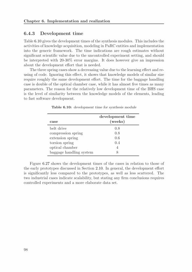
Chapter 6. Implementation and realization
6.4.3 Development time
Table 6.10 gives the development times of the synthesis modules. This includes theactivities of knowledge acquisition, modeling in PaRC entities and implementationinto the generic framework. The time indications are rough estimates withoutsignificant scientific value due to the uncontrolled experiment setting, and shouldbe interpreted with 20-30% error margins. It does however give an impressionabout the development effort that is needed.
The three spring cases show a decreasing value due to the learning effect and re-using of code. Ignoring this effect, it shows that knowledge models of similar sizerequire roughly the same development effort. The time for the baggage handlingcase is double of the optical chamber case, while it has almost five times as manyparameters. The reason for the relatively low development time of the BHS caseis the level of similarity between the knowledge models of the elements, leadingto fast software development.
Table 6.10: development time for synthesis module
casedevelopment time
(weeks)
belt drive 0.8compression spring 0.8extension spring 0.6torsion spring 0.4optical chamber 4baggage handling system 8
Figure 6.27 shows the development times of the cases in relation to those ofthe early prototypes discussed in Section 2.10. In general, the development effortis significantly less compared to the prototypes, as well as less scattered. Thetwo industrial cases indicate scalability, but stating any firm conclusions requirescontrolled experiments and a more elaborate data set.
98

6.4 Comparison
0
2
4
6
8
10
12
14
16
18
0 50 100 150 200 250
Development time
(weeks)
Parameters
prototypes
PaRC (literature)
PaRC (industrial)
Figure 6.27: synthesis module development time
99

Chapter 7Conclusions &
Recommendations
7.1 Conclusions
Mass-deployment of design automation applications in contemporary industry isnot prevented by the automation of models, but by the building of models fromexpert knowledge. The tacit nature and the diversity of the knowledge calls fora method and modeling standard that is independent of the design case at hand.This thesis proposes such a method for the scope of parametric engineering design.
This thesis provides a methodological translation of tacit and experience-basedknowledge into a model that is subsequently automated to generate multiple de-sign solutions. The development process of the software is prescribed to reducedevelopment effort and enable a modular software architecture.
The activities of the knowledge engineering method are prescribed indepen-dently of the design case and the automation algorithm. Knowledge engineeringbecomes an activity without the need to become a design expert or algorithmicexpert. Interview-style knowledge acquisition yields answers that are directly us-able to develop the model, and a generic algorithm is ready to process any modelthat meets the standard.
A key issue for efficient knowledge engineering and software development isthe consistency between knowledge acquisition and eventual automation: do notacquire something the algorithm cannot process. Consistency is guaranteed byprescribing the activities in terms of a single model of the design process andsynthesis knowledge, called PaRC. The model is used to standardize the inputand output of the knowledge engineering and software development activities.Standardization enables use of the same methods, procedures and algorithmswithin the applicability scope.
101

Chapter 7. Conclusions & Recommendations
The contribution to literature lies in the methodological documentation ofknowledge engineering of expert knowledge, and subsequent software developmentfor design automation. This thesis further aims to reduce the overall developmenteffort of the software program and make the process more predictable in terms ofthe activities to execute and the eventual functionality of the software. Withinscope, the method is generically applicable and scalable toward design problems ofhigher complexity in terms of number of parameters and topological complexity.
The overall development time of the design automation software is significantlydecreased while the design process itself is made explicit and modeled in a stan-dardized format. The benefits are most significant toward parametric problemswith predictable topologies.
Lifecycle aspects of the software are positively affected by the modularity ofthe software architecture and the knowledge model. The architecture modulescommunicate through generic interfaces that enable exchanging modules withoutaffecting the entire software. The knowledge model consists of self sustainingmodules (elements) that contain a part of the product model together with therelevant rules, independent of the algorithm. Modifications to the model are localand do not require algorithmic changes.
All development activities are prescribed in terms of the models of the designprocess and synthesis knowledge, resulting in several advantages during the sixdevelopment phases of design automation software:
1. decomposition: a design problem is first broken down into levels of abstrac-tion to discriminate between parameters of higher and lower importance.Software that aims to support engineering design and fit the original designprocess must acknowledge the division between issues of major and minorimportance.
Decomposing a design process into distinct layers of abstraction reduces thecomplexity and provides clear system boundaries for the modeling activities.A design problem has been cut down to manageable size because the expertshave to do it themselves. Experience led him/her to certain (tacit) models.Missing a model boundary not only leads to a larger problem that does notfit the original context, but the knowledge to solve the problem might bemissing because the expert does it differently.
A second decomposition step models the design process within a single layerof abstraction. The model is divided into sub-processes and sub-sets ofinformation. This phase further reduces complexity and provides systemboundaries on module level.
The model of the design process is determined predominantly by the analysismethod, and the analysis method is determined by the expert. The indirectmodeling method enables the expert to focus on his/her expertise, while theknowledge engineer receives the necessary information;
102

7.1 Conclusions
2. knowledge acquisition: the begin point of the knowledge acquisition phaseis an incomplete PaRC model, and the goal of this activity is to completethe model. The knowledge engineer knows what to look for, because thePaRC modeling entities are known in advance. The explicit nature of theentities improves communication between knowledge engineer and expert,making this phase efficient and fast.
Both industrial cases show relatively predictable content of knowledge rules.This indicates that experience relates to the model size, rather than therules;
3. modeling: a total of five standardized entities are used to model synthesisknowledge as a PaRC model. Using standardized modeling entities enablesefficient modular knowledge engineering of expert knowledge. The resultingmodels are easily modified and coupled, thanks to the modularity.
A verbal representation of the knowledge models serves as a knowledgecapturing document. The model describes the conclusion of experience:the model sizes and knowledge on the “how to move on”-aspect of designsynthesis. Directed graphs are used to graphically depict implicit designstrategies and flexibility of the problem solving capabilities;
4. automation: PaRC models of synthesis knowledge are automated with asingle algorithm. This removes the need for a custom algorithm for eachknowledge model.
Secondly, the algorithm provides the core functionality of the software,which means the characteristics (and limitations) are known almost imme-diately after modeling, but before software development. The design expertssee the end goal and its added value before implementation is started. Thisenables discussions and modifications when it is still easy to change.
The knowledge is organized in an agent-like manner. Agents in this senseare the PaRC entities of parameter and elements, who manage their ownvalue generation and validity thereof. The supervising algorithm guides thepopulation toward the endpoint: an embodiment. Solution generation isdone in a bottom-up manner: the modeling entities manage their own micro-knowledge (X-, R- and C-rules) to create a macro-solution (embodiment);
5. generic software development: the software architecture is made to mimicthe model of the design process. The interfaces between the sub-processesare made generic to allow modular software development. Modularity en-ables a toolkit-like software development process that reduces error sensi-tivity and required development effort for multiple cases;
6. user interface: the embodiment parameters are varied to explore designalternatives in the solution space. The performance parameters are used asquality measures for parameter sensitivity. Higher level understanding of
103
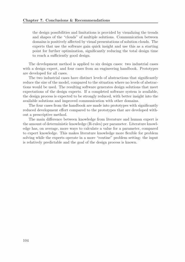
Chapter 7. Conclusions & Recommendations
the design possibilities and limitations is provided by visualizing the trendsand shapes of the “clouds” of multiple solutions. Communication betweendomains is positively affected by visual presentations of solution clouds. Theexperts that use the software gain quick insight and use this as a startingpoint for further optimization, significantly reducing the total design timeto reach a sufficiently good design.
The development method is applied to six design cases: two industrial caseswith a design expert, and four cases from an engineering handbook. Prototypesare developed for all cases.
The two industrial cases have distinct levels of abstractions that significantlyreduce the size of the model, compared to the situation where no levels of abstrac-tions would be used. The resulting software generates design solutions that meetexpectations of the design experts. If a completed software system is available,the design process is expected to be strongly reduced, with better insight into theavailable solutions and improved communication with other domains.
The four cases from the handbook are made into prototypes with significantlyreduced development effort compared to the prototypes that are developed with-out a prescriptive method.
The main difference between knowledge from literature and human expert isthe amount of deterministic knowledge (R-rules) per parameter. Literature knowl-edge has, on average, more ways to calculate a value for a parameter, comparedto expert knowledge. This makes literature knowledge more flexible for problemsolving while the experts operate in a more “routine” problem setting: the inputis relatively predictable and the goal of the design process is known.
104

7.2 Recommendations
7.2 Recommendations
A development method is described as an integration of a number of domains,guided by a central model of synthesis knowledge. First, several recommenda-tions for research directions of the individual domains are given to improve thedevelopment of design automation applications, depicted in Figure 7.1.
General recommendations to improve upon the “integrated domain”-approachfor software development are given afterward.
knowledgesource
designautomationsoftware
deco
mpo
sitio
n
know
ledg
e ac
quisition
mod
eling
auto
mat
ion
gene
ric sof
twar
e
deve
lopm
ent
user
inte
raction
Figure 7.1: knowledge domains and software development
7.2.1 Industrial decomposition
The applicability scope is widened if a broader range of design processes can bedecomposed and modeled. Examples are manufacturing related design processesand conceptual design. The use of static concepts (such as an analysis method)are found helpful as a starting point to prescribe the decomposition activity. Formanufacturing related processes, it seems interesting to start from the manufac-turing process to decompose the relevant information.
Conceptual design can be seen as a construction of conceptual form-functionentities, with the connections as (topological) degrees of freedom. Graph gram-mars are used to generate conceptual designs using grammars as form-functionentities [23]. A generic layout of a function entity can be used as static entity todecompose such design processes.
7.2.2 Knowledge acquisition
A wide range of interviewing techniques exists. The method of this thesis offersa clear begin point and end goal. Existing technique can be used to increaseefficiency and also document knowledge that is not needed for pure automation.If the core-knowledge is the knowledge required for automation of the designtask, the peripheral knowledge can explain why and relate to researches, studiesor important previous experiences.
105
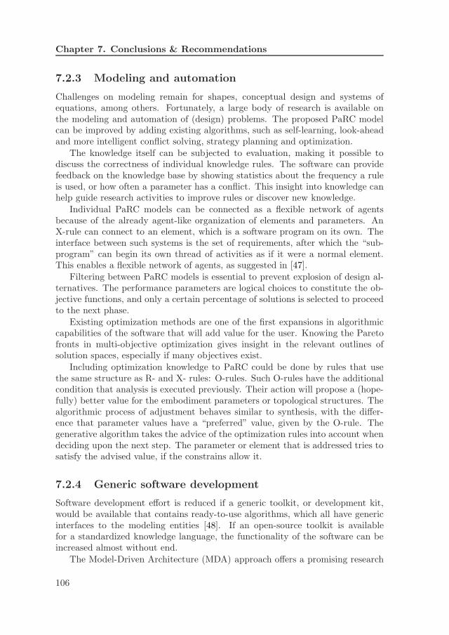
Chapter 7. Conclusions & Recommendations
7.2.3 Modeling and automation
Challenges on modeling remain for shapes, conceptual design and systems ofequations, among others. Fortunately, a large body of research is available onthe modeling and automation of (design) problems. The proposed PaRC modelcan be improved by adding existing algorithms, such as self-learning, look-aheadand more intelligent conflict solving, strategy planning and optimization.
The knowledge itself can be subjected to evaluation, making it possible todiscuss the correctness of individual knowledge rules. The software can providefeedback on the knowledge base by showing statistics about the frequency a ruleis used, or how often a parameter has a conflict. This insight into knowledge canhelp guide research activities to improve rules or discover new knowledge.
Individual PaRC models can be connected as a flexible network of agentsbecause of the already agent-like organization of elements and parameters. AnX-rule can connect to an element, which is a software program on its own. Theinterface between such systems is the set of requirements, after which the “sub-program” can begin its own thread of activities as if it were a normal element.This enables a flexible network of agents, as suggested in [47].
Filtering between PaRC models is essential to prevent explosion of design al-ternatives. The performance parameters are logical choices to constitute the ob-jective functions, and only a certain percentage of solutions is selected to proceedto the next phase.
Existing optimization methods are one of the first expansions in algorithmiccapabilities of the software that will add value for the user. Knowing the Paretofronts in multi-objective optimization gives insight in the relevant outlines ofsolution spaces, especially if many objectives exist.
Including optimization knowledge to PaRC could be done by rules that usethe same structure as R- and X- rules: O-rules. Such O-rules have the additionalcondition that analysis is executed previously. Their action will propose a (hope-fully) better value for the embodiment parameters or topological structures. Thealgorithmic process of adjustment behaves similar to synthesis, with the differ-ence that parameter values have a “preferred” value, given by the O-rule. Thegenerative algorithm takes the advice of the optimization rules into account whendeciding upon the next step. The parameter or element that is addressed tries tosatisfy the advised value, if the constrains allow it.
7.2.4 Generic software development
Software development effort is reduced if a generic toolkit, or development kit,would be available that contains ready-to-use algorithms, which all have genericinterfaces to the modeling entities [48]. If an open-source toolkit is availablefor a standardized knowledge language, the functionality of the software can beincreased almost without end.
The Model-Driven Architecture (MDA) approach offers a promising research
106

7.2 Recommendations
direction to further reduce (software) development cost and improve quality fora truly mass-deployment of software on different programming languages andplatforms. Technologies and techniques for model-driven software generation aredeveloped such as meta modeling, language definition and extension mechanisms(such as UML). If the MDA research efforts are combined with standardizedknowledge modeling, the boundary between generic code and specific code isfurther advanced. A domain specific modeling language (to define the knowledgemodels) is the starting point to develop software programs independently of theapplication’s platform.
7.2.5 User interaction
An intuitive and rewarding interaction between user and software is critical foracceptance in industry. Many things can be done once a cloud of solutions isgenerated. For instance: identification of the Pareto fronts, interactive cloudswhere different experts can select and de-select solutions. Multiple cross-sectionsof the solution space can be placed next to each other, and the performance of asingle solution is seen in all clouds simultaneously. Experts can ask for specificsensitivity studies, or optimization toward specific corners of the solution spaceby relaxing certain requirements.
Improvement of user interaction can also take the direction of interactiveknowledge bases. Users manage their knowledge bases without coding: the do-main of knowledge management is included into the development procedure.
7.2.6 General
A number of general recommendations for integrated software development meth-ods are suggested in figure 7.2, depicted as options A, B and C.
The first possibility (A) suggest the inclusion of other domains in the devel-opment process. For instance, Virtual Reality techniques can be included to offernew user interaction possibilities. Theories and models from cognitive design sci-ence can be helpful when following the same knowledge-guided approach as donein this thesis.
B signifies the use of alternative concepts within a domain, in a flexible manner.For example, a range of alternative automation and optimization algorithms canbe prepared and plugged in, depending on properties of the problem. This leadsto a toolkit-like approach with generic software modules, greatly advancing thecomputational power of the software that can be developed.
C suggest the development of a similar development method for other softwarefunctionalities, such as pure optimization or conceptual design. Different domainsmight be involved, but the approach to use a knowledge model as central conceptcan be used.
107
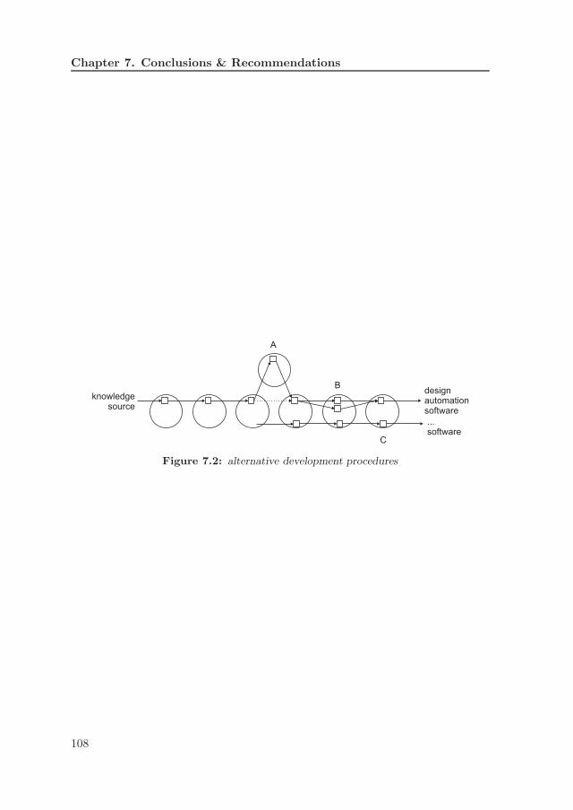
Chapter 7. Conclusions & Recommendations
knowledgesource
...software
A
B
C
designautomationsoftware
Figure 7.2: alternative development procedures
108

Acknowledgement
This thesis is part of the research project “Smart Synthesis Tools”, started in2005. The author gratefully acknowledges the support of the Dutch InnovationOriented Research Program “Integrated Product Creation and Realization (IOP-IPCR)” of the Dutch Ministry of Economic Affairs.
Professor Fred van Houten, dank voor onze leuke en nuttige discussies. Maar ookvoor de vrijheid die ik gekregen heb om de Wondere Wereld der Wetenschap temogen verkennen (vooral Las Vegas! En Kroatie was ook goed...).
I would also like to thank Professor Tomiyama and Professor Shea for theinteresting discussions about synthesis, science and design. Professor Wengenrothand Professor Bauchau for their excellent presentations at the right time. I thankyou all for giving me critical input and feedback during my research.
Tevens ben ik mijn dank verschuldigd aan alle heren uit de industrie die eenbijdrage hebben geleverd aan mijn promotie. Met name mijn begeleiders bij PAN-alytical en Vanderlande: Walter van den Hoogenhof, Rob de Lange en Roy vanPutten. Daarnaast dank ik ook de rest van de begeleidingscommissie voor dediscussies en feedback.
Furthermore, I would like to give some more personal thanks to a number people“without whom, none of this would have been possible”. First and foremost myparents, op wie de voorgaande frase in de meest letterlijke zin van toepassing is.Jullie steun en gezelschap is enorm belangrijk voor mij en heeft mij veel geholpen.Ik dank jullie, en hoop er nog lang van te kunnen genieten. Ik hoop dat het nieuwhuisje het warme hart van de familie wordt.
Kelly, mijn lieve vrouw, die aan mijn zijde stond gedurende de afgelopen vierjaar. Die al dat geneuzel over kennisregels heeft moeten aanhoren. Respect, liefdeen steun. Zonder jou...
109

Zus Maaike, die op enige afstand toch altijd dichtbij is. Hopelijk tot snel!Zusjes Annemiek en Leontien die beide ontzettend goede moeders zullen zijn, enmet hun natuurlijk Robbie en Joost, die fantastische vaders zullen zijn! Elsje, dieer gelukkig altijd is.
Mijn begeleider Frans Kokkeler, voor onze eindeloze gesprekken over evenzoveel onderwerpen. Ik ben ervan overtuigd dat jouw visie en stimulatie bepalendzijn geweest voor het resultaat van mijn promotie. Niet alleen voor de inhoud,maar ook zeker voor het plezier dat ik heb gehad tijdens de lange rit.
Snel daar achteraan komt Hans, die ook veel invloed heeft gehad op zowelde inhoud van mijn boekje als de weg er naartoe. De Paarse Bank, de gelijk-namige wereld, je weet wel. Hopelijk kunnen we samen nog veel projecten doen!Georg Still, dank voor je wiskundige kijk op mijn onderzoek en discussies over“marriage”-problemen!
Mijn collega’s van de vakgroep, die op gezette momenten een fijne discussieof gewoon slap geouwehoer mogelijk maakten. Bedankt voor de goede sfeer, diezich hopelijk uitstrekt in de toekomst! Een speciaal dankwoord voor de zingendeAjoo’s: Gijs, Frederik en Irene. Onze muzikale ontdekkingstocht was leuk enverhelderend: zingen is niets voor mij.
Wessel, mijn walking-talking helpdesk en bovenal goede vriend. De enige diemeteen weet waar in mijn LATEX-code ik een uitroeptekentje, apostrofje dan welminteken ben vergeten. Ongelofelijk. Enorm bedankt. Ontzettend leuk om samente studeren, promoveren en hierna docenteren.
Rutger, ook jou dank ik voor je aanwezigheid tijdens de middelbare school,studie en promotie tijd. Op de volgende!
Juan, een fijne collega en vriend. Leuke discussies, let’s keep it up! Maerten,the code-magician. MarcoO, el valorisator! Njels, de baas. Goed dat jullie erwaren, zijn en zullen zijn! En de rest van de Ajoo’s natuurlijk: Matthhijss, Jan,Denise-Denise, Boris und Der Krein. Maar ook in het Westen des Landsch, waarhet sjaaltje van Hanz vrolijk wappert: Valentina.
De raggende stammetjes: Wout, Jens & Mijke, Richard en Thijz. Het HoogeNoorden, de Spiegel/Images. Ze roepen. Wout: bedankt voor je hulp met devoorkant! Looking good...
Natuurlijk mag de 67-clan niet vergeten worden: Nannoekie, Vincent, Germ,Jorien, Jop, Ronaldicus P., Casper Joost. De Groene Draeck-mannen: Sieger,Rutger en Robbie (zum zweiten Mal), Ronald en C! Vaker oud&nieuw diners enfeesten!
Nou is het niet de bedoeling dat ik nog meer bladzijden volschrijf, dus ik moeter een eind aan breien. Ik heb genoten en hoop jullie allemaal snel weer te zien.Voor iedereen die ik niet met naam genoemd heb: ontzettend bedankt en tot snel!
110
List of References
[1] S.L. Ahire and P. Dreyfus. The impact of design management and processmanagement on quality: an empirical investigation. Journal of OperationsManagement, 18: 549-575, 2000. [cited at p. 1]
[2] E.K. Antonsson and J. Cagan. Formal Engineering Design Synthesis. Cam-bridge University Press, 2001. [cited at p. 14, 17]
[3] Roman Bartak. Constraint programming: in pursuit of the holy grail. Pro-ceedings of WDS99, Prague, 1999. [cited at p. 15, 36, 39]
[4] J. Bento, B. Feijo, and D.L. Smith. Engineering design knowledge representa-tion based on logic and objects. Computers and Structures, 63 - 5: 1015-1032,1997. [cited at p. 31]
[5] F. Bolognini, A.A. Seshia, and K. Shea. Exploring the application of amult-domain simulation-based computational synthesis method in mems de-sign. Proceedings of the 16th International Conference on Engineering De-sign, ICED’07, 2007. [cited at p. 14]
[6] J. Cagan, M.I. Campbell, S. Finger, and T. Tomiyama. A framework forcomputational design synthesis: Models and applications. Journal of Com-puting and Information Science in Engineering, 5: 171-181, 2005. [cited at p. 6,
14]
[7] M.I. Campbell, J. Cagan, and K. Kotovsky. Agent-based synthesis of electro-mechanical design configurations. Journal of Mechanical Design, 122/61,2000. [cited at p. 14]
[8] M.I. Campbell, J. Cagan, and K. Kotovsky. The a-design approach to manag-ing automated design synthesis. Research in Engineering Design, 14: 12-24,2003. [cited at p. 14]
111
[9] A. Chakrabarti. Engineering Design Synthesis: Understanding, Approachesand Tools, volume ISBN 1852334924. Springer Verlag, London, 2002.[cited at p. 14]
[10] H. Draijer and F.G.M. Kokkeler. Heron’s synthesis engine applied to linkagedesign- the philosophy of watt software. Proceedings of the Design Engineer-ing Technical Conferences and Computer and Information in EngineeringConference, Montreal 2002, DETC2002/MECH-34373, 2002. [cited at p. 19]
[11] N.F.O. Evbuomwan, S. Sivaloganathan, and A. Jebb. A survey of designphilosophies, models, methods and systems. Journal of Engineering Manu-facture, 210: 301-320, 1996. [cited at p. 26]
[12] E.A. Feigenbaum. How the “what” becomes the “how”. communications ofthe ACM, 39, 1996. [cited at p. 17]
[13] E.A. Feigenbaum. Some challenges and grand challenges for computationalintelligence. Journal of the ACM, 50, 2003. [cited at p. 17]
[14] D. Fensel. The Knowledge Acquisition and Representation Language, KARL.Kluwer Academic Publishers, 1995. [cited at p. 13, 17]
[15] W. Geerdes. Smart design of baggage handling systems. Master’s the-sis, University of Twente, Faculty of Engineering Design, OPM-816, 2007.[cited at p. 78]
[16] J.S. Gero and U. Kannengiesser. The situated function-behaviour-structureframework. Design Studies, 25(373-391), 2004. [cited at p. XV, 11, 12]
[17] R. Green. Cad manager survey 2004: Part 2. Cadalyst (www.cadalyst.com),2004. [cited at p. 1]
[18] R.M. Henderson and K.B. Clark. Architectural innovation: the reconfigu-ration of existing product technologies and the failure of established firms.Administrative Science Quarterly, 35(1990): 9-30, 1990. [cited at p. 1]
[19] V. Hubka and W.E. Eder. Design Science. Springer-Verlag, 1996. [cited at p. 9]
[20] S. Kirkpatrick, C.D. Gelatt jr., and M.P. Vecchi. Optimization by simulatedannealing. Science, 13: 671-980, 1983. [cited at p. 15]
[21] T.D. Kuczmarski. Managing new products: competing through excellence.in: Rao199, pp. 83-84, 1998. [cited at p. 1]
[22] V. Kumar. Algorithms for constraint satisfaction problems: a survey. AImagazine, 13(1): 32-44, 1992. [cited at p. 15, 28]
112
[23] T. Kurtoglu and M.I. Campbell. A graph grammar based framework forautomated concept generation. Proceedings of the International Design Con-ference 2006, pp. 61-68, 2006. [cited at p. 14, 105]
[24] R.T. Marler and J.S. Arora. Survey of multi-objective optimization methodsfor engineering. Structural and multidisciplinary optimization, 26: 369-395,2004. [cited at p. 15]
[25] W. Matek, D. Muhs, H. Wittel, and M. Becker. Roloff-Matek machine-onderdelen. Academic Service Schoonhoven, 1996. [cited at p. 20, 84]
[26] Ohsuga In: C. McMahon and J. Brown. CAD/CAM principles, prac-tise and manufacturing management. Addison-Wesley Longman Ltd, 1998.[cited at p. XV, 26, 27]
[27] MOKA consortium Melody Stokes. Managing Engineering Knowledge:MOKA. Professional Engineering Publication, 2001. [cited at p. 16, 18]
[28] J. Miedema, M.C. van der Voort, and F.J.A.M. van Houten. Application ofsynthetic environments in product design. CIRP Journal of ManufacturingScience and Technology, 1: 159-164, 2009. [cited at p. 19]
[29] J. Moss, J. Cagan, and K. Kotovsky. Learning from design experience in anagent-based design system. Research in Engineering Design, 15: 77-92, 2004.[cited at p. 14]
[30] N. Nijenmanting. Towards a synthesis tool for baggage handling systems.Master’s thesis, University of Twente, Faculty of Engineering Design, OPM-844, 2008. [cited at p. 78]
[31] P.Y. Papalambros and D.J. Wilde. Principles of Optimal Design- Modelingand Computation. Cambridge University press, 2000. [cited at p. 6]
[32] K.S. Pawar and J.C.K.H. Riedel. A survey of cad use in the uk mechani-cal engineering industry. International Journal of Computer Applications inTechnology, 9(4): 219-228, 1996. [cited at p. 2]
[33] C.K. Prahalad and K. Lieberthal. The end of corporate imperialism. HarvardBusiness Review, 2003. [cited at p. 1]
[34] S.S. Rao, A. Nahm, S. Zhengzhong, X. Deng, and A. Syamil. Artificialintelligence and expert systems applications in new product development- asurvey. Kluwer Academic Publishers, 1999. [cited at p. 1]
[35] B. Raphael and I.F.C. Smith. Fundamentals of Computer-Aided Engineering.Wiley, 2003. [cited at p. 17]
[36] R. Rothwell. Toward the fifth-generation innovation process. InternationalMarketing Review, 11(1): 7-31, 1994. [cited at p. 1]
113

[37] O.W. Salomons. Computer support in the Design of Mechanical Products.Copyprint 2000, 1995. [cited at p. 18]
[38] K. Schilstra. Towards continuous knowledge engineering. PhD Thesis. 2003.[cited at p. 17]
[39] W.O. Schotborgh, F.G.M. Kokkeler, H. Tragter, M.J. Bommhoff, andF.J.A.M. van Houten. A generic synthesis algorithm for well-defined para-metric design. Proceedings of the 18th CIRP Design Conference, 2008.[cited at p. 29]
[40] W.O. Schotborgh, F.G.M. Kokkeler, H. Tragter, and F.J.A.M. van Houten. Abottom-up approach for automated synthesis tools in the engineering designprocess. Proceedings of International Design Conference 2006, pp. 349-356,2006. [cited at p. 19, 55]
[41] W.O. Schotborgh, H. Tragter, F.G.M. Kokkeler, F.J.A.M. van Houten, andT. Tomiyama. Towards a generic model of smart synthesis tools. Proceedingsof the CIRP Design Seminar 2007, 2007. [cited at p. 19]
[42] T.W. Simpson, J.D. Peplinksi, P.N. Koch, and J.K. Allen. Metamodels forcomputer-based engineering design: survey and recommendations. Engineer-ing with Computers, 2001. [cited at p. 2]
[43] P. Sridharan and M.I. Campbell. A grammar for function structures. Pro-ceedings of the ASME Design Engineering Technical Conference, 3: 41-55,2004. [cited at p. 14]
[44] A.C. Starling. Performance-based computational synthesis of parametric me-chanical systems. PhD thesis, 2004. [cited at p. 14]
[45] S. Studer and V.R Benjamins. Knowledge engineering: principles and meth-ods. Data & Knowledge Engineering, 25: 161-197, 1998. [cited at p. 18, 28]
[46] M. Tideman. Scenario Based Product Design. PhD Thesis. PrintpartnersIpskamp, 2008. [cited at p. 19]
[47] T. Tomiyama and W.O. Schotborgh. Yet another model of design synthe-sis. Proceedings of the 16th International Conference on Engineering Design,ICED’07, pp. 83-84, 2007. [cited at p. 26, 106]
[48] H. Tragter, W.O. Schotborgh, M.H.L. Roring, and F.J.A.M. van Houten.Generic data architecture for parametric synthesis systems. Proceedings ofCIRP Design Conference 2008, Enschede, 2008. [cited at p. 58, 106]
[49] D.G. Ullman. Toward the ideal mechanical engineering design support sys-tem. Research in Engineering Design, 13(2): 55-64, 2002. [cited at p. 2]
114

[50] Y. Umeda and T. Tomiyama. Fbs modeling: Modeling scheme of functionfor conceptual design. 1995. [cited at p. 10]
[51] C. Vempati and M.I. Campbell. A graph grammar approach to generateneural network topologies. 2007 Proceedings of the ASME Design Engineer-ing Technical Conferences and Computers and Informatics in EngineeringConference, 6: 79-89, 2008. [cited at p. 14]
[52] W. Visser. Designing as construction of representations: A dynamic view-point in cognitive design research. Human-Computer Interaction, 21: 103-152, 2006. [cited at p. 23, 35, 36, 96]
[53] B.J. Wielinga, A.T. Schreiber, and J.A. Breuker. Kads: a modelling approachto knowledge engineering. Knowledge Acquisition, 4: 5-53, 1992. [cited at p. 13]
[54] H. Yoshikawa. General design theory and a cad system. Man-Machine Com-munication in CAD/CAM, 1981. [cited at p. 10]
[55] M. Yoshioka, Y. Umeda, H. Takeda, Y. Shimomura, Y. Nomaguchi, andT. Tomiyama. Physical concept ontology for the knowledge intensive en-gineering framework. Advanced Engineering Informatics, 18: 95-113, 2004.[cited at p. 12]
[56] W.J. Zhang, Y. Lin, and N. Sinha. On the function-behavior-structure modelfor design. Canadian Design Engineering Network conference 2005, CD,2005. [cited at p. XV, 10, 11]
115


Appendices
117


Appendix ASynthesis knowledge
A.1 Optical chamber
This section states the knowledge base for synthesis, as implemented in the pro-totype for optical chamber design.
A.1.1 Elements and parameters
The elements of the optical chamber are stated in table A.1 and the parametersin table A.2. Figure A.1 illustrates the parameters concerning the optical axis.
Table A.1: optical chamber, elements
name description
OC optical chamberT tubeDet detectorS sampleC casingD diaphragmDSP diaphragm set primary sideDSS diaphragm set secondary side
119

Table A.2: optical chamber, parameters
type name description
scenario Smat sample materialTA tube surface areaTmat tube materialDetA detector surface area
embodiment T(x,y) tube positionTα tube orientationDet(x,y) detector positionDetα detector orientationS(x,y) sample positionSd sample diameterSα sample orientationSt sample thicknessCmat casing materialCd casing diameterCL casing lengthCt casing thicknessDmat diaphragm materialDt diaphragm thicknessDO diaphragm aperture openingD(x,y) diaphragm aperture centerDα diaphragm orientationDk diaphragm knife edge
auxiliary OCβP angle primary axisOCLP length primary axisOCβS angle secondary axisOCLP length secondary axisOC(x,y) optical center (x, y)OCEmax maximum energyOCEmin minimum energyOCNT total number of diaphragmsOCNP number of primary diaphragmsOCNS number of secondary diaphragmsOCmidpoint focus on sample midpoint (y/n)SV A sample view areaSstandard sample standard (y/n)DSPsample DSP against sample (y/n)DSPtube DSP against tube (y/n)DSSsample DSS against sample (y/n)
Continued on next page
120

Table A.2 – continued from previous page
type name description
DSSdetector DSS against detector (y/n)
OCßP
St
Dk
CL
Cd
TA Tα
DetA
Detα
Ct
OCßS
Sd
OC(x, y)
OCLSOCLP
Dt
Dxx
y
Figure A.1: optical axis
A.1.2 X-rules
The X-rules are stated in set A.1. The required information is included on theleft side of the arrow, and any parameter values that are resolved are indicatedon the right hand side.
OCexpands−−−−−→T, Det, S, C, DSP, DSS (A.1)
DSP (DSPsample, DSPtube, OCNP ,
S(x), Sd, T(x), Tα, TA)expands−−−−−→D(x)
DSS(DSSsample, DSSdetector, OCNS ,
S(x), Sd, Det(x), Detα, DetA)expands−−−−−→D(x)
A.1.3 R-rules
The R-rules are stated in equation set (A.2).
OC(x,y) = f(OCmidpoint, S(x,y), St) →OC(x,y) (A.2)
OCNT = OCNP + OCNS →OCNT , OCNP , OCNS
OCEmax = f(Tmat) →OCEmax
121
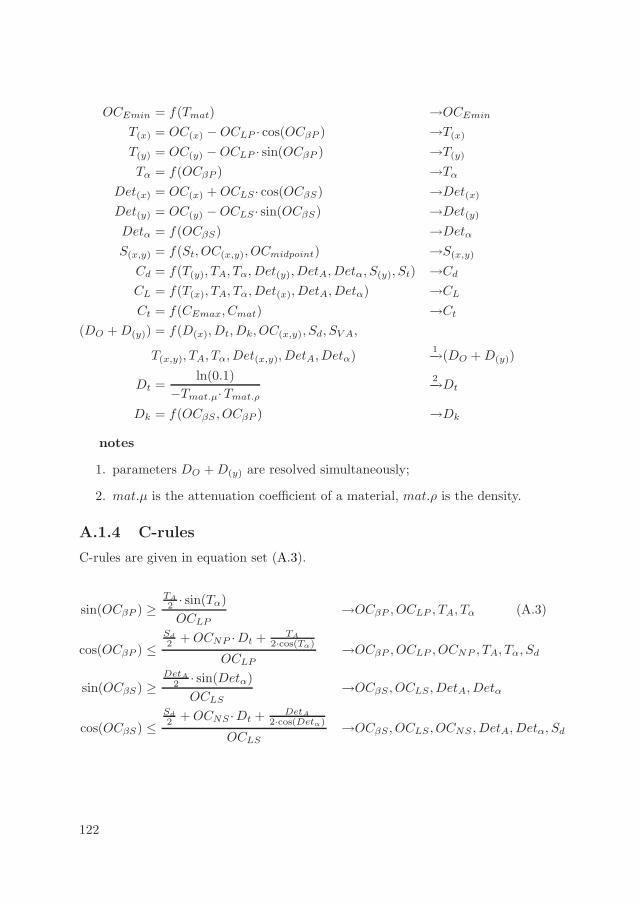
OCEmin = f(Tmat) →OCEmin
T(x) = OC(x) − OCLP · cos(OCβP ) →T(x)
T(y) = OC(y) − OCLP · sin(OCβP ) →T(y)
Tα = f(OCβP ) →Tα
Det(x) = OC(x) + OCLS · cos(OCβS) →Det(x)
Det(y) = OC(y) − OCLS · sin(OCβS) →Det(y)
Detα = f(OCβS) →Detα
S(x,y) = f(St, OC(x,y), OCmidpoint) →S(x,y)
Cd = f(T(y), TA, Tα, Det(y), DetA, Detα, S(y), St) →Cd
CL = f(T(x), TA, Tα, Det(x), DetA, Detα) →CL
Ct = f(CEmax, Cmat) →Ct
(DO + D(y)) = f(D(x), Dt, Dk, OC(x,y), Sd, SV A,
T(x,y), TA, Tα, Det(x,y), DetA, Detα)1−→(DO + D(y))
Dt =ln(0.1)
−Tmat.µ·Tmat.ρ
2−→Dt
Dk = f(OCβS , OCβP ) →Dk
notes
1. parameters DO + D(y) are resolved simultaneously;
2. mat.µ is the attenuation coefficient of a material, mat.ρ is the density.
A.1.4 C-rules
C-rules are given in equation set (A.3).
sin(OCβP ) ≥TA
2 · sin(Tα)
OCLP
→OCβP , OCLP , TA, Tα (A.3)
cos(OCβP ) ≤Sd
2 + OCNP ·Dt + TA
2·cos(Tα)
OCLP
→OCβP , OCLP , OCNP , TA, Tα, Sd
sin(OCβS) ≥DetA
2 · sin(Detα)
OCLS
→OCβS , OCLS , DetA, Detα
cos(OCβS) ≤Sd
2 + OCNS ·Dt + DetA
2·cos(Detα)
OCLS
→OCβS , OCLS , OCNS , DetA, Detα, Sd
122

A.2 Baggage handling systems
This section presents the synthesis knowledge as implemented in the prototypefor baggage handling system (BHS) design.
The discussion on elements, parameters, X-rules and R-rules is divided intofive categories, table A.3.
Table A.3: categories
category description
PFD process main processes of a BHSEquipmentGroupSet contains multiple equipment groupsEquipmentGroup contains multiple pieces of equipmentEquipment handles the baggageMiscellaneous elements Area, BeltNetwork and BaggageFlow
A.2.1 Elements
In total there are 51 elements, as summarized in table A.4 and elaborated furtherin this section.
Table A.4: elements
name quantity
PFD process 10EquipmentGroupSet 9EquipmentGroup 9Equipment 19Miscellaneous 4
PFD process The BHS functional design is described with the 10 PFDprocess elements stated in table A.5.
123

Table A.5: PFD process elements
name description
CheckIn check-in belt (BHS input)HBS12 hold baggage screening level 1 + 2HBS34 hold baggage screening level 3 + 4HBS5 hold baggage screening level 5SuspectBagSplit split baggage flow into cleared and suspectBagRemoval removes bag from system (BHS output)DetermineID determine the ID tag on baggageIDReadSplit split baggage flow into ID read and not readManualCoding manual determination of ID tag on baggageSortation sort baggage to chutes (BHS output)
Equipment/Group/Set Each PFD process element contains an elementXXEquipmentGroupSet, where XX is the name of the PFD process. Withinthis set, there are multiple elements XXEquipmentGroup. The only exception isCheckIn, which does not have EquipmentGroupSet or EquipmentGroup. For theothers, this introduces 19 elements.
The EquipmentGroup element contains the actual equipment that operate onthe baggage flow. The list of 19 equipment elements is given in table A.6.
Table A.6: equipment elements
PFD process name description
general Belt contains baggage flowFeedInBelt feed baggage into equipmentDivert12 split one flow into twoMerge21 merge two flow into one
HBS12 ScreeningMachineLevel1 level 1 screeningScreeningMachineLevel2 level 2 screening
HBS34 ScreeningMachineLevel3 level 3 screeningScreeningMachineLevel4 level 4 screening
HBS5 ScreeningMachineLevel5 level 5 screeningSuspectBagSplit SuspectBagDivertInput split flow into
suspect and clearedSuspectBagDivertExitSuspect divert exit, suspectSuspectBagDivertExitCleared divert exit, cleared
Continued on next page
124

Table A.6 – continued from previous page
PFD process name description
BagRemoval BagRemovalEquipment removes baggage from BHSDetermineID DetermineIDMachine reads ID tags on baggageIDReadSplit IDReadDivertInput splits flow into
ID read and ID not readIDReadDivertExitRead divert exit, ID readIDReadDivertExitNotRead divert exit, ID not read
ManualCoding ManualCodingStation reads ID tags manuallySortation Sorter sorts baggage to exit chutes
Miscellaneous Contains the 4 elements of table A.7.
Table A.7: miscellaneous elements
name description
Area the “mother-element” that contains the PFD processesBeltNetwork collects incoming baggage flow for PFD processBaggageFlow contains the beltsNetwork redistributes the baggage flow over belts
A.2.2 Parameters
BHS synthesis knowledge contains 204 parameters, summarized in table A.8 andelaborated in the following sections.
Table A.8: parameters
name quantity
PFD process 55EquipmentGroupSet 9EquipmentGroup 9Equipment 128Miscellaneous 3
125
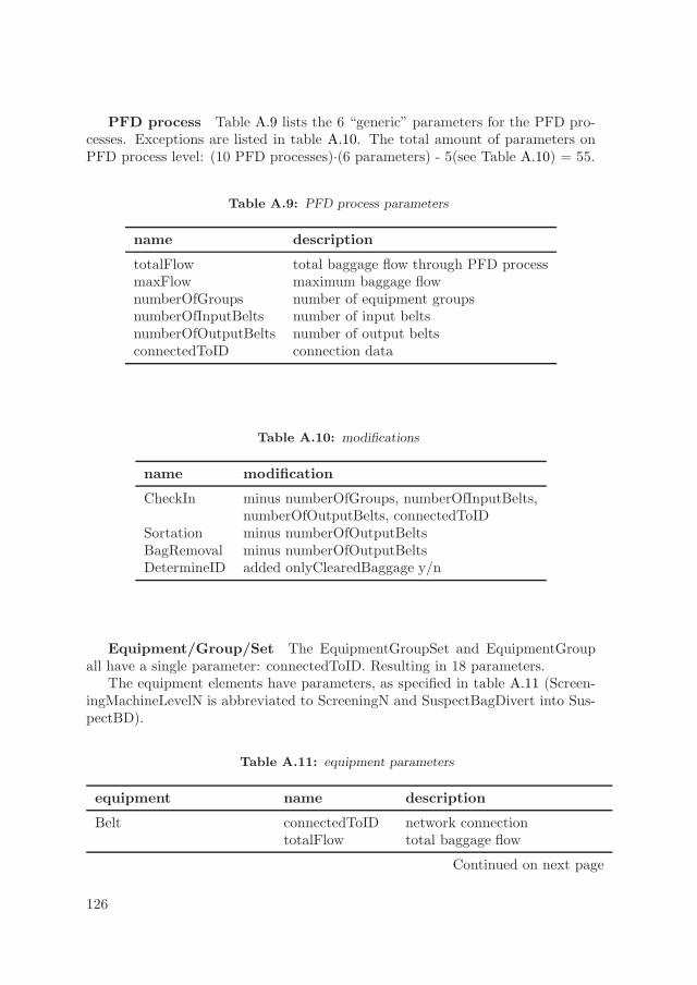
PFD process Table A.9 lists the 6 “generic” parameters for the PFD pro-cesses. Exceptions are listed in table A.10. The total amount of parameters onPFD process level: (10 PFD processes)·(6 parameters) - 5(see Table A.10) = 55.
Table A.9: PFD process parameters
name description
totalFlow total baggage flow through PFD processmaxFlow maximum baggage flownumberOfGroups number of equipment groupsnumberOfInputBelts number of input beltsnumberOfOutputBelts number of output beltsconnectedToID connection data
Table A.10: modifications
name modification
CheckIn minus numberOfGroups, numberOfInputBelts,numberOfOutputBelts, connectedToID
Sortation minus numberOfOutputBeltsBagRemoval minus numberOfOutputBeltsDetermineID added onlyClearedBaggage y/n
Equipment/Group/Set The EquipmentGroupSet and EquipmentGroupall have a single parameter: connectedToID. Resulting in 18 parameters.
The equipment elements have parameters, as specified in table A.11 (Screen-ingMachineLevelN is abbreviated to ScreeningN and SuspectBagDivert into Sus-pectBD).
Table A.11: equipment parameters
equipment name description
Belt connectedToID network connectiontotalFlow total baggage flow
Continued on next page
126

Table A.11 – continued from previous page
equipment name description
maxFlow maximum baggage flowsuspect amount of suspect baggagecleared amount of cleared baggageIDRead amount of ID read baggageIDNotRead amount of ID not read baggage
FeedInBelt idem Belt idem BeltDivert12 connectedToID network connection
ratio ratio left/right baggage flowMerge21 connectedToID1 network connection
connectedToID2 network connectionScreening1 connectedToID network connection
totalFlow total baggage flowmaxFlow maximum baggage flowsuspect amount of suspect baggagecleared amount of cleared baggageIDRead amount of ID read baggageIDNotRead amount of ID not read baggagepercentCleared percentage of baggage cleared
Screening2 idem Screening1 idem Screening1Screening3 idem Screening1 idem Screening1Screening4 idem Screening1 idem Screening1Screening5 idem Screening1 idem Screening1SuspectBDInput idem Belt idem BeltSuspectBDExitSuspect idem Belt idem BeltSuspectBDExitCleared idem Belt idem BeltBagRemovalEquipment connectedToID network connection
totalFlow total baggage flowmaxFlow maximum baggage flow
DetermineIDMachine idem Belt idem BeltpercentageRead percentage of ID tags read
IDReadDivertInput idem Belt idem BeltIDReadDivertExitRead idem Belt idem BeltIDReadDivertExitNotRead idem Belt idem BeltManualCodingStation idem Belt idem Belt
percentageRead percentage of ID tags readSorter idem Belt idem Belt
numberOfExits number of exit chuteslength length of the sorter
127

The equipment parameters: (11 · 7 Belt parameters) + ( 5 · 8 Screening1parameters) + 11 = 128 parameters.
Miscellaneous Only the element BaggageFlow has three parameters: num-berOfBelts, connectedToID and totalFlow.
A.2.3 X-rules
A total of 46 X-rules are used to construct the topological tree: table A.12, anddiscussed in categories. The X-rules also resolve the connectedToID parameterfor their sub-elements.
Table A.12: X-rules
category quantity
PFD process 27EquipmentGroupSet 9EquipmentGroup 9Equipment 0Miscellaneous 1
PFD process PFD processes have, in general, three X-rules:
1. expand and connect BeltNetwork, EquipmentGroupSet and BaggageFlow;
2. expand and connect Belts in BeltNework (to collect baggage flow from up-stream PFD processes);
3. expand and connect Belts in BaggageFlow (the output side).
Exceptions are CheckIn, which does not have the second type, and BagRemovaland Sortation, which do not have the third type. In total, that brings 27 X-ruleson PFD process level.
Equipment/Group/Set All EquipmentGroupSet elements have one R-rule to expand and connect with the required number of EquipmentGroups. Inturn, these elements expand and connect their specific configuration of equipment.For these elements there are in total 18 X-rules.
Miscellaneous BeltNetwork expands its topology with two BaggageFlowsand a Network in between: one X-rules.
128

A.2.4 R-rules
120 R-rules are required for synthesis of BHS design: table A.13 and discussed incategories.
Table A.13: R-rules
category quantity
PFD process 35EquipmentGroupSet 0EquipmentGroup 0Equipment 83Miscellaneous 2
PFD process The “generic” R-rules for PFD processes are four in total,table A.14.
Table A.14: parameters and R-rules
parameter R-rule
totalFlow sum the flows inside BaggageFlow of BeltNetworknumberOfGroups divide totalFlow with maxFlow of equipmentsnumberOfInputBelts count number of input belts in
first equipment of each EquipmentGroupnumberOfOutputBelts count number of output belts in
last equipment of each EquipmentGroup
Exceptions are CheckIn, which has no R-rules, and BagRemoval which has nooutput belts. This results in 10 · 4 - 5 = 35 R-rules.
Equipment/Group/Set The elements EquipmentGroupSet and Equipment-Group have no R-rules, but equipment does. The five “generic” R-rules for equip-ment concern the baggage flow. Each flow (suspect, cleared, ID read and ID notread) is retrieved from the upstream equipment and processed, if necessary (e.g.suspect becomes cleared for a screening machine). The parameter totalFlow is asummation of the suspect and cleared baggage flow.
Exceptions are:
1. BaggageRemovalEquipment: only one R-rule for totalFlow: resolved byretrieving from upstream equipment;
129
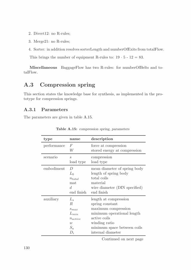
2. Divert12: no R-rules;
3. Merge21: no R-rules;
4. Sorter: in addition resolves sorterLength and numberOfExits from totalFlow.
This brings the number of equipment R-rules to: 19 · 5 - 12 = 83.
Miscellaneous BaggageFlow has two R-rules: for numberOfBelts and to-talFlow.
A.3 Compression spring
This section states the knowledge base for synthesis, as implemented in the pro-totype for compression springs.
A.3.1 Parameters
The parameters are given in table A.15.
Table A.15: compression spring, parameters
type name description
performance F force at compressionW stored energy at compression
scenario s compressionload type load type
embodiment D mean diameter of spring bodyL0 length of spring bodyntotal total coilsmat materiald wire diameter (DIN specified)end finish end finish
auxiliary Ls length at compressionR spring constantsmax maximum compressionLmin minimum operational lengthnactive active coilsw winding ratioSa minimum space between coilsDi internal diameter
Continued on next page
130

Table A.15 – continued from previous page
type name description
De external diameterLc bloc lengthsc bloc compressionFmax force at bloc compressionσ stress at bloc compressionσmax maximum allowed stress
A.3.2 R-rules
R-rules are given in equation set (A.4).
R =mat.G
8· d4
D3·nactive
→R, D, nactive (A.4)
R =F
s→R, F, s
W =R· s2
2→W, R, s
σmax = 0.45· (mat.Rm1− mat.Rm2· log(d)) →σmax
Lmin = Lc + Sa →Lmin, Lc, Sa
L0 = sc + Lc →L0, sc, Lc
d = k1· 3
√
F ·De1−→d
ntotal = nactive + factor2−→ntotal, nactive
Sa = (0.0015· D2
d+ 0.1· d)·nactive
= 0.02· (D + d)·nactive
= 1.5·Sa
= 2·Sa3−→Sa, D, nactive
w =D
d→w, D
D =Di + De
2→D, Di, De
Di = D − d →Di, D
De = D + d →De, D
Fmax = R· sc →Fmax, R, sc
131

σ = Fmax·D
0.4· d3→σ, Fmax, D
Lc = (ntotal + factor)· d 4−→Lc, ntotal
L0 = s + Ls →L0, s, Ls
L0 = smax + Lmin →L0, smax, Lmin
notes
1. k1 depends on material, and the calculated wire diameter is matched to thenearest in the DIN specification;
2. factor depends on material, either 2 or 1.5;
3. these rules are considered together, taking into account the load type andmaterial. The resolved parameters are Sa, D or nactive;
4. factor depends on material and end finish.
A.3.3 C-rules
C-rules are given equation set (A.5).
d ≥ mat.dmin →d, mat (A.5)
d ≤ mat.dmax →d, mat
D ≤ mat.Dmax →D, mat
L0 ≤ mat.Lmax →L0, mat
nactive ≥ mat.nmin →nactive, mat
w ≥ mat.wmin →w, mat
w ≤ mat.wmax →w, mat
σ ≤ σmax →σ, σmax
F ≤ Fmax →F, Fmax
Lc ≤ Lmin →Lc, Lmin
Lmin ≤ L0 →Lmin, L0
s ≤ smax →s, smax
L0 ≥ d·ntotal →L0, d, ntotal
Ls ≥ Lmin →Ls, Lmin
smax ≤ sc →smax, sc
132

A.4 Extension spring
This section states the knowledge base for synthesis, as implemented in the pro-totype for extension springs.
A.4.1 Parameters
Table A.16: extension spring, parameters
type name description
performance F force at extensionW stored energy at extension
scenario s extensionload type load type
embodiment D mean diameter of spring bodyL0 total lengthntotal total coilsnactive active coilsmat materiald wire diameter (DIN specified)end finish end finish typeF0 pre-load
auxiliary R spring constantLk length of active spring bodyDi internal diameterDe external diameterLh length of end-finishesL length at extensionsmax maximum extensionLmax length at maximum extensionFmax force at maximum extensionσ stress at maximum extensionσmax maximum allowed stressw winding ratio
133

A.4.2 R-rules
R-rules are given in equation set (A.6).
R =mat.G
8· d4
D3·nactive
→R, D, nactive (A.6)
R =F − F0
s→F, F0, R, s
W =R· s2
2→W, R, s
σ = Fmax·D
0.4· d3→σ, D, Fmax
σmax = 0.45· (mat.Rm1− mat.Rm2· log(d)) →σmax
Lmax = L0 + smax →Lmax, L0, smax
L = L0 + s →L, L0, s
Lh = factor·Di1−→Lh
d = k1· 3
√
F ·De2−→d
ntotal = nactive + factor3−→ntotal, nactive
w =D
d→w, D
D =Di + De
2→D, Di, De
Di = D − d →Di, D
De = D + d →De, D
Fmax = R· smax + F0 →Fmax, R, smax, F0
Lk = nactive· d →Lk, nactive
L0 = Lk + 2·Lh →L0, Lk, Lh
notes
1. factor depends on end finish type and wire diameter;
2. k1 depends on material and the calculated wire diameter is matched to thenearest in the table;
3. factor depends on end finish.
134
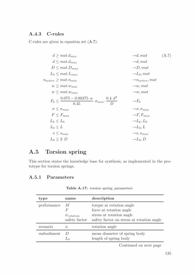
A.4.3 C-rules
C-rules are given in equation set (A.7).
d ≥ mat.dmin →d, mat (A.7)
d ≤ mat.dmax →d, mat
D ≤ mat.Dmax →D, mat
L0 ≤ mat.Lmax →L0, mat
nactive ≥ mat.nmin →nactive, mat
w ≥ mat.wmin →w, mat
w ≤ mat.wmax →w, mat
F0 ≤ 0.075 − 0.00375·w0.45
·σmax·0.4· d3
D→F0
σ ≤ σmax →σ, σmax
F ≤ Fmax →F, Fmax
Lk ≤ L0 →Lk, L0
L0 ≤ L →L0, L
s ≤ smax →s, smax
L0 ≥ 2·D →L0, D
A.5 Torsion spring
This section states the knowledge base for synthesis, as implemented in the pro-totype for torsion springs.
A.5.1 Parameters
Table A.17: torsion spring, parameters
type name description
performance M torque at rotation angleF force at rotation angleσrotation stress at rotation anglesafety factor safety factor on stress at rotation angle
scenario α rotation angle
embodiment D mean diameter of spring bodyL0 length of spring body
Continued on next page
135
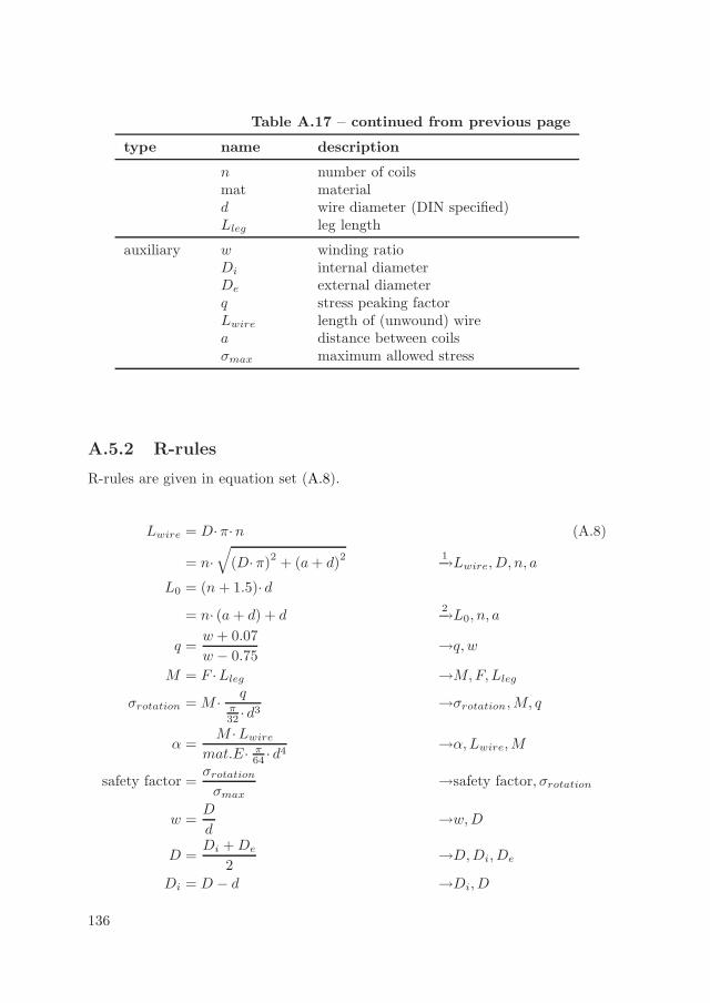
Table A.17 – continued from previous page
type name description
n number of coilsmat materiald wire diameter (DIN specified)Lleg leg length
auxiliary w winding ratioDi internal diameterDe external diameterq stress peaking factorLwire length of (unwound) wirea distance between coilsσmax maximum allowed stress
A.5.2 R-rules
R-rules are given in equation set (A.8).
Lwire = D·π·n (A.8)
= n·√
(D·π)2
+ (a + d)2 1−→Lwire, D, n, a
L0 = (n + 1.5)· d
= n· (a + d) + d2−→L0, n, a
q =w + 0.07
w − 0.75→q, w
M = F ·Lleg →M, F, Lleg
σrotation = M · qπ32 · d3
→σrotation, M, q
α =M ·Lwire
mat.E· π64 · d4
→α, Lwire, M
safety factor =σrotation
σmax
→safety factor, σrotation
w =D
d→w, D
D =Di + De
2→D, Di, De
Di = D − d →Di, D
136
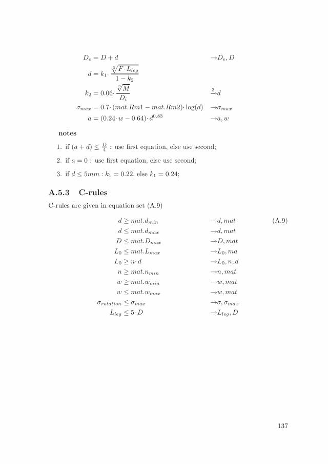
De = D + d →De, D
d = k1·3
√
F ·Lleg
1 − k2
k2 = 0.06·3√
M
Di
3−→d
σmax = 0.7· (mat.Rm1 − mat.Rm2)· log(d) →σmax
a = (0.24·w − 0.64)· d0.83 →a, w
notes
1. if (a + d) ≤ D4 : use first equation, else use second;
2. if a = 0 : use first equation, else use second;
3. if d ≤ 5mm : k1 = 0.22, else k1 = 0.24;
A.5.3 C-rules
C-rules are given in equation set (A.9)
d ≥ mat.dmin →d, mat (A.9)
d ≤ mat.dmax →d, mat
D ≤ mat.Dmax →D, mat
L0 ≤ mat.Lmax →L0, ma
L0 ≥ n· d →L0, n, d
n ≥ mat.nmin →n, mat
w ≥ mat.wmin →w, mat
w ≤ mat.wmax →w, mat
σrotation ≤ σmax →σ, σmax
Lleg ≤ 5·D →Lleg, D
137
