knowledge discovery and data mining using demographic and

IN DEGREE PROJECT MEDICAL ENGINEERING,SECOND CYCLE, 30 CREDITS

, STOCKHOLM SWEDEN 2018

Knowledge Discovery and Data mining using demographic and clinical data to diagnose heart disease.

JAVIER FERNÁNDEZ SÁNCHEZ

KTH ROYAL INSTITUTE OF TECHNOLOGYSCHOOL OF ENGINEERING SCIENCES IN CHEMISTRY, BIOTECHNOLOGY AND HEALTH

i

Abstract

Cardiovascular disease (CVD) is the leading cause of morbidity, mortality, premature death and reduced quality

of life for the citizens of the EU. It has been reported that CVD represents a major economic load on health care sys-

tems in terms of hospitalizations, rehabilitation services, physician visits and medication. Data Mining techniques

with clinical data has become an interesting tool to prevent, diagnose or treat CVD. In this thesis, Knowledge Dis-

covery and Data Mining (KDD) was employed to analyse clinical and demographic data, which could be used to

diagnose coronary artery disease (CAD). The exploratory data analysis (EDA) showed that female patients at an el-

derly age with a higher level of cholesterol, maximum achieved heart rate and ST-depression are more prone to be

diagnosed with heart disease. Furthermore, patients with atypical angina are more likely to be at an elderly age with

a slightly higher level of cholesterol and maximum achieved heart rate than asymptotic chest pain patients. More-

over, patients with exercise induced angina contained lower values of maximum achieved heart rate than those

who do not experience it. We could verify that patients who experience exercise induced angina and asymptomatic

chest pain are more likely to be diagnosed with heart disease. On the other hand, Logistic Regression, K-Nearest

Neighbors, Support Vector Machines, Decision Tree, Bagging and Boosting methods were evaluated by adopting

a stratified 10 fold cross-validation approach. The learning models provided an average of 78-83% F-score and a

mean AUC of 85-88%. Among all the models, the highest score is given by Radial Basis Function Kernel Support

Vector Machines (RBF-SVM), achieving 82.5% ± 4.7% of F-score and an AUC of 87.6% ± 5.8%. Our research con-

firmed that data mining techniques can support physicians in their interpretations of heart disease diagnosis in

addition to clinical and demographic characteristics of patients.

ii

Aknowledgements

First, I would like to thank BYON8 AB for giving the opportunity to let me be involved in an amazing and pas-

sionate world of a health-tech start-up. I would like to reserve particular gratification to Matias and Josef for their

support and guidance through these intensive months.

Thanks to all my classmates who became friends, with a special thanks to Jakob who made my days a bit easier

here in the north by eating tortillas every weekend.

Special thanks to my colleagues who have supported me during this journey and to Kassim Caratella who is still

the best international manager superstar.

Another special thanks for my previous supervisor and friend Inma from Universidad Rey Juan Carlos (URJC)

who provided me support and advice with regular meetings.

Last but not least, my very special thanks to my mother who is always there no matter what. Thanks also to the

rest of my family (sister, father and Mario) who support me every day in this adventure in the North. THANKS.

iii

“If you have an apple and I have an apple and we exchange these apples

then you and I will still each have one apple. But if you have an idea

and I have an idea and we exchange these ideas, then each of us will have two ideas"

– George Bernard Shaw

Contents

Abstract . . . . . . . . . . . . . . . . . . . . . . . . . . . . . . . . . . . . . . . . . . . . . . . . . . . . . . . . . . . . i

Aknowledgements . . . . . . . . . . . . . . . . . . . . . . . . . . . . . . . . . . . . . . . . . . . . . . . . . . . . . ii

1 Introduction and Objectives 2

1.1 Context and Motivation . . . . . . . . . . . . . . . . . . . . . . . . . . . . . . . . . . . . . . . . . . . . . . . 2

1.2 Objectives . . . . . . . . . . . . . . . . . . . . . . . . . . . . . . . . . . . . . . . . . . . . . . . . . . . . . . . 3

2 Database and pre-processing 4

2.1 The Data Set . . . . . . . . . . . . . . . . . . . . . . . . . . . . . . . . . . . . . . . . . . . . . . . . . . . . . . 4

2.2 Data pre-processing . . . . . . . . . . . . . . . . . . . . . . . . . . . . . . . . . . . . . . . . . . . . . . . . . 7

3 Exploratory Data Analysis 13

3.1 Violin plots of relevant features . . . . . . . . . . . . . . . . . . . . . . . . . . . . . . . . . . . . . . . . . . . 13

3.2 Scatter plots of relevant features . . . . . . . . . . . . . . . . . . . . . . . . . . . . . . . . . . . . . . . . . . 14

4 Machine Learning approaches and parameter tuning 17

4.1 Tuning parameters . . . . . . . . . . . . . . . . . . . . . . . . . . . . . . . . . . . . . . . . . . . . . . . . . . 17

4.2 Single methods . . . . . . . . . . . . . . . . . . . . . . . . . . . . . . . . . . . . . . . . . . . . . . . . . . . . 18

4.3 Ensemble methods . . . . . . . . . . . . . . . . . . . . . . . . . . . . . . . . . . . . . . . . . . . . . . . . . . 19

4.3.1 Voting classifiers . . . . . . . . . . . . . . . . . . . . . . . . . . . . . . . . . . . . . . . . . . . . . . . 19

4.3.2 Bootstrap aggregating (Bagging) . . . . . . . . . . . . . . . . . . . . . . . . . . . . . . . . . . . . . . 19

4.3.3 Random Forest and Extremely Randomized Trees . . . . . . . . . . . . . . . . . . . . . . . . . . . . 20

4.3.4 Boosting . . . . . . . . . . . . . . . . . . . . . . . . . . . . . . . . . . . . . . . . . . . . . . . . . . . . 20

4.3.5 Adaptive Boosting (AdaBoost) . . . . . . . . . . . . . . . . . . . . . . . . . . . . . . . . . . . . . . . 20

4.3.6 Gradient Tree Boosting Classifier (GTB) . . . . . . . . . . . . . . . . . . . . . . . . . . . . . . . . . . 21

4.3.7 eXtreme Gradient Boosting classifier (XGBoost) . . . . . . . . . . . . . . . . . . . . . . . . . . . . . 21

5 Results and discussion 23

5.1 Model validation . . . . . . . . . . . . . . . . . . . . . . . . . . . . . . . . . . . . . . . . . . . . . . . . . . . 23

5.2 Comparison with previous research . . . . . . . . . . . . . . . . . . . . . . . . . . . . . . . . . . . . . . . . 29

iv

CONTENTS 1

6 Conclusions and Future Work 31

6.1 Conclusions . . . . . . . . . . . . . . . . . . . . . . . . . . . . . . . . . . . . . . . . . . . . . . . . . . . . . . 31

6.2 Future Work . . . . . . . . . . . . . . . . . . . . . . . . . . . . . . . . . . . . . . . . . . . . . . . . . . . . . . 32

A State-of-the-art 33

A.1 Cardiovascular Diseases . . . . . . . . . . . . . . . . . . . . . . . . . . . . . . . . . . . . . . . . . . . . . . . 33

A.2 Clinical Decision Support . . . . . . . . . . . . . . . . . . . . . . . . . . . . . . . . . . . . . . . . . . . . . . 35

A.2.1 Telehealth . . . . . . . . . . . . . . . . . . . . . . . . . . . . . . . . . . . . . . . . . . . . . . . . . . . 36

A.2.2 Predictive Analytics . . . . . . . . . . . . . . . . . . . . . . . . . . . . . . . . . . . . . . . . . . . . . . 37

A.3 Data Mining and Machine Learning . . . . . . . . . . . . . . . . . . . . . . . . . . . . . . . . . . . . . . . . 38

A.3.1 Model Validation . . . . . . . . . . . . . . . . . . . . . . . . . . . . . . . . . . . . . . . . . . . . . . . 40

A.3.2 Cross validation in Machine Learning . . . . . . . . . . . . . . . . . . . . . . . . . . . . . . . . . . . 40

A.3.3 Bias Variance trade-off . . . . . . . . . . . . . . . . . . . . . . . . . . . . . . . . . . . . . . . . . . . . 41

A.3.4 Previous research - predictive analytics . . . . . . . . . . . . . . . . . . . . . . . . . . . . . . . . . . 42

A.3.5 Bootstrap aggregating (bagging) . . . . . . . . . . . . . . . . . . . . . . . . . . . . . . . . . . . . . . 45

A.3.6 When does Bagging work well? . . . . . . . . . . . . . . . . . . . . . . . . . . . . . . . . . . . . . . . 46

A.3.7 Boosting methods . . . . . . . . . . . . . . . . . . . . . . . . . . . . . . . . . . . . . . . . . . . . . . 46

A.4 Ethics and datasets . . . . . . . . . . . . . . . . . . . . . . . . . . . . . . . . . . . . . . . . . . . . . . . . . . 47

A.5 Evaluation Metrics . . . . . . . . . . . . . . . . . . . . . . . . . . . . . . . . . . . . . . . . . . . . . . . . . . 48

B Gantt Diagram 50

B.1 Gantt Diagram . . . . . . . . . . . . . . . . . . . . . . . . . . . . . . . . . . . . . . . . . . . . . . . . . . . . . 51

Bibliography 52

Chapter 1

Introduction and Objectives

This Chapter describes the scope of the project. First, it depicted the clinical context and motivation and sub-

sequently, it discusses the main purpose of this Thesis.

1.1 Context and Motivation

The global population has raised concerns about the current economical climate. The impact on health has

had an increase in burden over the last few years. Healthcare systems should address different challenges such as

universal access to quality healthcare by means of adequate allocation of financial resources between healthcare

activities (preventive or curative care) and healthcare providers (hospitals or primary care centers).

According to Eurostat [1], the level of current expenditure in Sweden is positioned at third place with the highest

ratios of current healthcare expenditure in Europe. This is equivalent to 11.1% of gross domestic product (GDP).

Particularly, 38.6% of the current healthcare expenditure in Sweden is used in Hospitals, while 18.5% is applied to

residential long-term care facilities and 24.2% to providers of primary care centers [1].

On the other hand, healthcare systems have to adapt themselves to meet new demands: improvement in knowl-

edge, new medical technology, change in healthcare policies due to developments in demographic terms (life ex-

pectancy) and tackle different diseases [2]. The above reasons have helped physicians and providers to accomplish

better welfare. Conversely, it is also believed to be a key driver of healthcare spending.

Cardiovascular diseases (CVD) are a major cause of mortality in the European Union (EU), which require more

resources in terms of time and economical. Problems of the circulatory system place a considerable burden on

healthcare systems and government expenditure. Statistics from the latest released reports states that in 2014 there

were 1.83 million deaths resulting from diseases of the circulatory systems, equivalent to 37.1% of all deaths. Deaths

in advanced age i.e., >65 years old are more common than any other cause, although such age discrepancies are

more prominent in diseases of the circulatory system [3]. Hence, it is a priority to prevent and control these diseases

by achieving accurate diagnosis decisions promptly (reducing diagnosis time and improving diagnosis accuracy).

To conclude, there is a real need to support the "modernization" of this new age. More effort should be placed to

2

CHAPTER 1. INTRODUCTION AND OBJECTIVES 3

create a better public health, with an improved effectiveness and access within healthcare systems. These strategies

will focus on reducing the impact of sickness-health in individuals by boosting the introduction of new technolo-

gies for improved cost-effectiveness and care delivery.

1.2 Objectives

There is nowadays an increasing concern about health care, since the development of technology which has led

to an improvement of welfare and lifestyle. However, the current economic situation has called for a development

of a sustainable health care system by applying the available resources efficiently. In this study, we focus on patients

who suffer chronic conditions, particularly those with coronary heart disease (CAD) due to their significance: high

percentage of prevalence among the population and high cost which they requires.

The aim of this project is to perform a complete knowledge discovery and data mining (KDD) approach to

correctly classify CAD as a diagnosis in unseen examples. To achieve this, the following sub-objectives are also

proposed:

• To examine, clean, select and transform numerical and categorical features for this study.

• To develop a descriptive analysis of the most relevant features selected and pre-processed from the previous

stage.

• To perform machine learning (ML) algorithms and optimizing these techniques.

• To compare different classification algorithms to correctly classify diagnosis of heart disease in unseen ex-

amples.

Chapter 2

Database and pre-processing

This chapter commenced in Section 2.1 by presenting and explaining both the data set provided by different

clinical centers. Later in Section 2.2, we described the issues we found when applying the first exploratory analysis

and how we prepared our data towards building the machine learning algorithms.

2.1 The Data Set

The implementation of digital solutions within the clinical scope in the current society has become a powerful

tool in organizational terms (annotation legibility, content security, paper files removal). The relation between the

physician and the clinic information has changed: ideally, now physicians can access clinical history of patients

due to the constant data availability.

In this study, data from the University California Irvin Machine Learning Repository has been used. This data

dates from 1988 and is publicly available. The data comes from four different sources:

• Cleveland Clinic Foundation: Robert Detrano, M.D., Ph.D.

• Hungarian Institute of Cardiology, Budapest: Andras Janosi, M.D.

• V.A. Medical Center, Long Beach, CA: Robert Detrano, M.D., Ph.D.

• University Hospital, Zurich, Switzerland: William Steinbrunn, M.D

The sources will be referred to as Cleveland, Hungarian, Long Beach VA and Switzerland datasets for simplicity.

The number of samples/patients per source are described below in Table 2.1a. We can observe that the dataset is

imbalanced. There is around 55.3% of patients diagnosed with heart disease and 44.7% of patients without heart

disease (See Table 2.1b). Therefore, we should choose the most relevant metric to evaluate the machine learning

models which will be applied to such data.

4

CHAPTER 2. DATABASE AND PRE-PROCESSING 5

#Samples Dataset303 Cleveland294 Hungary123 Switzerland200 Long Beach VA920 Total

(a)

Heart DiseaseSex Diagnosis No Diagnosis Total

Female 144 50 194Male 267 458 725Total 411 508 919

(b)

Table 2.1: Number of samples. (a) Number of samples per dataset, (b) Number of samples per sex and diagnosis ofheartdisease.

Each database provides 5 numerical features (age, chol, trestbps, thalach and oldpeak) and 8 categorical fea-

tures (sex, cp, fbs, restecg, exang, slope and thal). Furthermore, the target variable is also categorical (heartdisease).

The structure of each dataset is shown in Figure 2.1.


Dataset

Patient1

Age (age) [years]

Sex (sex)

{sex0: Female

sex1: Male

Chest Pain Type (cp)

cp1: Typical Angina

cp2: Atypical Angina

cp3: Non-anginal pain

cp4: Asymptomatic

Resting Blood Pressure [mm/Hg] (trestbps)

Serum Cholesterol [mm/dl] (chol)

Fasting Blood Sugar (fbs)

{fbs0: fbs < 120 mg/dL

fbs1: fbs > 120 mg/dL

Resting Electrocardiographic Results (restecg)

restecg0: Normal

restecg1: ST-T wave abnormality

restecg2: Left ventricular hypertrophy

Maximum Heart Rate Achieved [bps] (thalach)

Exercise Induced Angina (exang)

{exang0: No exercise induced angina

exang1: Exercise induced angina

ST depression induced by exercise relative to rest [mm] (oldpeak)

Slope of the peak exercise ST segment (slope)

slope1: Upslopping

slope2: Flat

slope3: Downsloping

Number of major vessels (0-3) colored by flourosopy (ca)

Thalium test (thal)

thal0: Normal

thal1: Fixed defect

thal2: Reversable defect

Diagnosis of heart disease (heartdisease)

heartdisease0: <50% diameter narrowing

in any major vessel

heartdisease1: >50% diameter narrowing

in any major vessel

Patient2

Patient3

...

PatientN

Pati ent i where i=1..Npatients

Figure 2.1: Structure of each dataset with its corresponding original attributes or features


2.2 Data pre-processing

Data exploratory analysis revealed that the number of samples per source is very scarce. This is why we decided

to collect every sample from each source and create a final database based on Cleveland, Hungary, Switzerland and

Long Beach VA data sources.

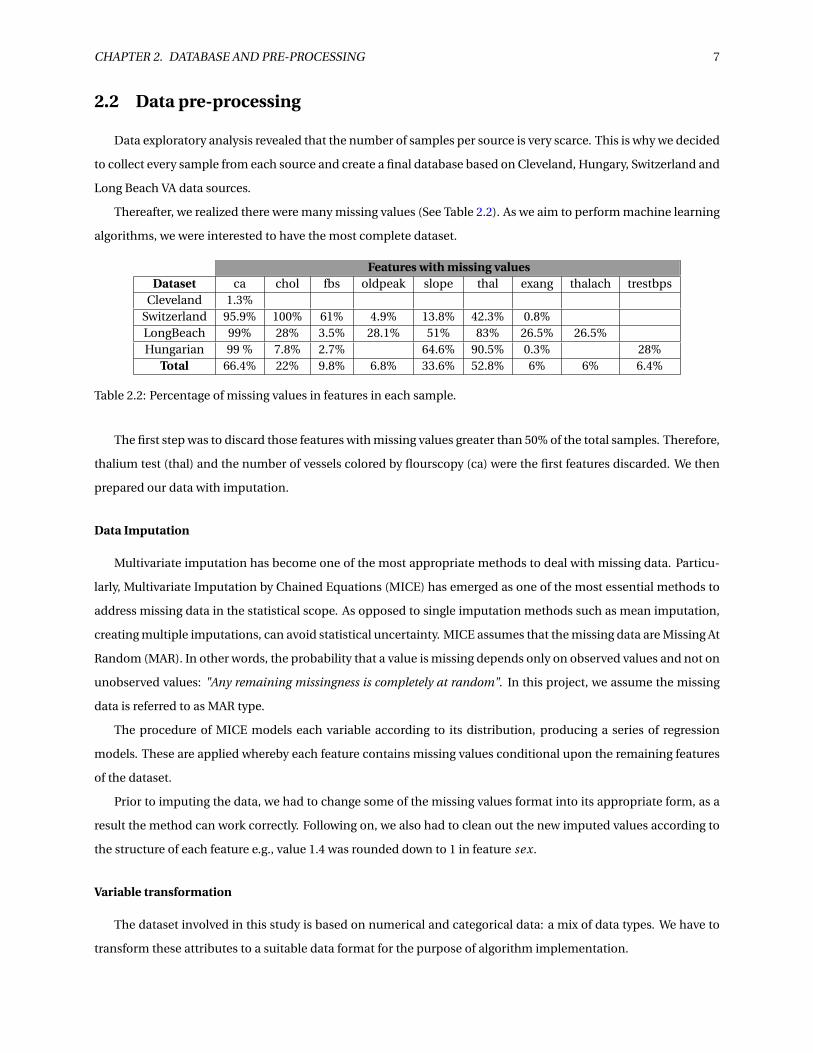
Thereafter, we realized there were many missing values (See Table 2.2). As we aim to perform machine learning

algorithms, we were interested to have the most complete dataset.

Features with missing valuesDataset ca chol fbs oldpeak slope thal exang thalach trestbps

Cleveland 1.3%Switzerland 95.9% 100% 61% 4.9% 13.8% 42.3% 0.8%LongBeach 99% 28% 3.5% 28.1% 51% 83% 26.5% 26.5%Hungarian 99 % 7.8% 2.7% 64.6% 90.5% 0.3% 28%

Total 66.4% 22% 9.8% 6.8% 33.6% 52.8% 6% 6% 6.4%

Table 2.2: Percentage of missing values in features in each sample.

The first step was to discard those features with missing values greater than 50% of the total samples. Therefore,

thalium test (thal) and the number of vessels colored by flourscopy (ca) were the first features discarded. We then

prepared our data with imputation.

Data Imputation

Multivariate imputation has become one of the most appropriate methods to deal with missing data. Particu-

larly, Multivariate Imputation by Chained Equations (MICE) has emerged as one of the most essential methods to

address missing data in the statistical scope. As opposed to single imputation methods such as mean imputation,

creating multiple imputations, can avoid statistical uncertainty. MICE assumes that the missing data are Missing At

Random (MAR). In other words, the probability that a value is missing depends only on observed values and not on

unobserved values: "Any remaining missingness is completely at random". In this project, we assume the missing

data is referred to as MAR type.

The procedure of MICE models each variable according to its distribution, producing a series of regression

models. These are applied whereby each feature contains missing values conditional upon the remaining features

of the dataset.

Prior to imputing the data, we had to change some of the missing values format into its appropriate form, as a

result the method can work correctly. Following on, we also had to clean out the new imputed values according to

the structure of each feature e.g., value 1.4 was rounded down to 1 in feature sex.

Variable transformation

The dataset involved in this study is based on numerical and categorical data: a mix of data types. We have to

transform these attributes to a suitable data format for the purpose of algorithm implementation.


Numerical attributes from any dataset may be measured in a different way (different units). Therefore, the

features must be re-scaled in order to have the same importance when applying any machine learning algorithm.

Transforming numerical data: Min-Max scaler

The first processing of numerical data applied in this dataset is re-scaling to a fixed range - [−1,1]. This can

suppress the effect of outliers.

A min-max scaling is performed by the equation stated below:

Xnor m = X −Xmi n

Xmax −Xmi n(2.1)

Transforming numerical data: Standardization or Z-score normalization

This way the features are re-scaled in such a way that its properties will be the same a standard distribution

with µ= 0 andσ= 1. where µ is the mean (average) andσ is the standard deviation from the mean; standard scores

(also called z scores) of the samples are calculated as follows:

z = x −µσ

(2.2)

This is fundamental for some machine learning schemes. For instance, algorithms which often use gradient

descent (logistic regression or SVM). Some features may be in different scales, and some weights may update faster

than others since the feature values x j play an important role in the weight updates:

∆w j =−η ∂J

∂w j= η∑

i(t (i ) −o(i ))x(i )

j (2.3)

So that w j := w j +∆w j , where η is the learning rate and t the target class label and o the actual output.

Other examples where this normalization might be useful are K-Nearest Neighbors and clustering algorithms

which use euclidean distance measures.

Transforming categorical data: one-hot-encoding (OHE)

We can distinguish between two types of categorical data: nominal and ordinal. The first type does not have

any sense of order among discrete categorical values, while it does for ordinal data.

In our dataset, we just have nominal data since there is no notion of order among the categorical values in any

feature.

The idea here is to transform the categorical features into a more representative numerical format which can

be understood by the machine learning algorithms. Thus, first the categorical values should be transformed into

numerical labels and then applying some encoding scheme to these values.

Considering we have the numeric representation of any categorical attribute with m labels, the OHE scheme,

encodes the feature into m binary attributes which can only contain a value of 0 (absence) or 1 (presence). For


instance, if we have a categorical feature named chest pain type which contains 4 values: typical angina, atypical

angina, non-anginal pain and asymptomatic. The first step will be to transform these values into numeric repre-

sentation, and then generating 4 new features which would be cp1, cp2, cp3 and cp4 containing only 0 and 1 values

in each new feature.

Feature selection

In several practical data mining situations, there are many attributes or features to be handled and most of them

are clearly redundant or irrelevant. Many machine learning techniques try to select the most appropriate features,

but this often leads to model performance deterioration.

This can be improved by discarding those irrelevant attributes and keep the ones the models actually use. The

advantages of feature selection are many. Reducing dimensionality speeds up the computation of those algorithms

as well as providing a more compact and easy interpretable representation of the target. Moreover, it also reduces

the problem of overfitting, where a learned machine learning model is tied up too closely to the training data.

Therefore, it outperforms better on training data than on new unseen instances.

In this study, we tried several feature selection approaches along with machine learning techniques to identify

the most relevant attributes of the dataset.

Attribute clustering can be useful for creating models. It allows analysts to see the relationship of these at-

tributes and a particular extent of choice. The idea behind hierarchical clustering is pretty simple: initially each

attribute is considered as its own cluster. The algorithm then finds the two closest clusters in terms of distance or

similarity measure, merge them and continues doing this until there is just one cluster left.

Figure 2.2 shows a bottom-up approach hierarchical clustering that recursively merges features following the

same basis as described previously. It uses the single linkage criterion which determines the distance (correlation)

to use between sets of attributes.

We can observe that some of the features are correlated with each other: (cp4 - exang1), (exang0 - thal ach)

and (exang1 - ol d peak) are one of the set of attributes with strongest correlation with each other.


Figure 2.2: Dendrogram of the resulting cluster hierarchy (agglomerative) which has chosen the most relevantattributes. The heatmap shows the extent of correlation between features.

Furthermore, we also used Recursive Feature Elimination (RFE). The procedure works as follows: an external

estimator (a machine learning scheme) assigns weights to features e.g., the coefficients in a linear model, then

it selects those features by recursively considering smaller sets of features. Thus, first the estimator is trained and

then it selects those features with more importance and discard those irrelevant attributes from the set. It continues

until the desired number of features is eventually reached.

Due to the imbalance of our dataset, we perform this algorithm with 10-fold stratified cross validation. We used

two estimators, a support-vector machine (SVM) scheme with linear kernel and a random forest (RF) estimator.


(a) (b)

Figure 2.3: Mean accuracy of a RFE 10-fold stratified cross validation approach considering different number offeatures using (a) Random Forest and (b) Support vector machines (linear kernel).

According to Figure 2.3, we can claim that the number of features selected with RF as estimator, which gives

the best score, is 10. ag e, sex0, cp2, cp4, tr estbps, chol , r estecg0, thal ach, exang0 and ol d peak. On the other

hand, SVM-linear estimator provides 17 features selected which provide the best cross-validation score. However,

we can see there is a peak when the number of features selected is ten which gives a slightly lower score than the

best. These 10 features are: sex0, sex1, cp2, cp4, chol , f bs0, thal ach, exang0, exang1, ol d peak.

We also applied tree-based methods to evaluate the importance in a classification task. Importance in this

context is often called "Gini Importance" or "Mean Decrease Impurity" and it is defined as the total decrease in

node impurity, weighted by the probability of reaching that particular node, which is approximated by the number

of samples reaching that node. Then it is averaged over all trees of the ensemble [4].

(a) (b)

Figure 2.4: Feature ranking using (a) Extra Trees and (b) Random Forest along with their inter-trees variability.

In addition to Random Forest, the other estimator considered in this case is: Extremely randomized trees, which

is a meta estimator which fits a number of randomized decision trees on the training data and use averaging to

improve the predictive accuracy and control overfitting.


According to Figure 2.4, we can see that the most relevant features for both estimators are chol , thal ach, ag e,

cp4, ol d peak, tr estbps, exang0 and exang1 then the rest contains very little importance and becomes constant

for the remaining features.

Considering all of these methods which gives different results, we tried selecting different features and verified

the best performance is given by discarding the following features: sl ope1,2,3, f bs0,1, cp1,3 and r estecg0,1,2.

Hence the final dataset contains, in addition to the target feature hear tdi sease, the following: ag e, sex0,1,

cp2,4, tr estbps, chol , thal ach, exang0,1 and ol d peak.

Chapter 3

Exploratory Data Analysis

An exploratory analysis is an essential step towards performing high quality research. This step of the study has

been performed along with the data pre-processing. It was essential to verify how the missing data was distributed

and what approach was better to address. Moreover, it was also useful to see how similar are some feature distribu-

tions with each other. Section 3.1 of this chapter refers to how numerical features are distributed across different

values of categorical data. Later in Section 3.2, we showed the distribution of each sample in each numerical feature

across different categories of categorical features.

We resolved that cp1,3 (typical angina and non-anginal pain) were discarded according from our feature selec-

tion algorithms. According to the figures illustrated in this Chapter (See sub-figures in Figure 3.1 and Figure 3.2).

This was done due to the limited amount of available samples from this level in chest pain feature (See middle

column subfigures in Figure 3.2)

3.1 Violin plots of relevant features

In this section we showed the distribution of quantitative data (age, cholesterol, maximum heart rate achieved,

resting blood pressure and ST Depression induced by exercise relative to rest) across different levels of the sex,

chest pain type and exercise induced angina features. Each subfigure illustrated a kernel density estimation (KDE)

of the underlying distribution of each level in each categorical feature, making a clear distinction of diagnosing

heart disease. The dotted lines describes the median (middle line) and the quartiles (both sides). Note that KDE is

influenced by the sample size and features with relatively small samples might look misleadingly smooth. Also, we

determined some outliers (thin line at the tails of each violin).

According to each subfigure in Figure 3.1 we can claim that female patients are diagnosed with heart disease

at an elderly age, higher level of cholesterol, maximum heart rate achieved and ST depression than male patients.

Female patients accounted for 21.1% of the population considered in the dataset while male patients proportion is

89.9% (See Table 2.1b).

Chest pain type could give us a good idea about which patients are diagnosed with heart disease, in particu-

13

CHAPTER 3. EXPLORATORY DATA ANALYSIS 14

lar, those patients with atypical angina or it asymptomatic. We discovered that asymptomatic patients suffer heart

disease at a similar elderly age than atypical angina but the latter one is more likely to be at an elderly age; pa-

tients with atypical angina are diagnosed heart disease at a bit higher cholesterol levels and maximum heart rate

achieved than patients with no symptoms in their chest; atypical angina contains similar resting blood pressure to

asymptomatic patients, but the distribution is slightly skewed to higher values. On the other hand, we determined

that there are some outliers in asymptomatic patients and that atypical angina distribution is much more smoother

than asymptomatic patients.

Furthermore, we concluded that the maximum heart rate for patients with exercise angina is lower than for

those ones who do not experience it. Younger patients are more prone to suffer exercise induced angina.

3.2 Scatter plots of relevant features

Showing each observation at each level of the categorical variable is also very useful to check which features are

more discriminatory to diagnose heart disease and also to check if there are enough samples in each feature to take

it into consideration for our models. Before feature selection, we revealed the discarded attributes have very scarce

observations.

According to Figure 3.2, we could state that male patients have a quite good extent of discrimination of heart

disease. In addition to this, we determined that asymptomatic chest pain patients are more prone to be diagnosed

with heart disease. Moreover, patients who experienced exercise induced angina are also prone to suffer heart

disease. We concluded that the discarded features e.g., typical angina does not contain many observations. On

the other hand, features with not so many observations e.g, female patients showed a much smoother feature

distribution as expected.


(a) (b) (c)

(d) (e) (f)

(g) (h) (i)

(j) (k) (l)

(m) (n) (o)

Figure 3.1: Distribution of (a), (b) and (c) age; (d), (e) and (f) cholesterol; (g), (h) and (i) maximum heart rate achieved, (j),(k) and (l) resting blood pressure; (m), (n) and (o) ST-depression induced by exercise relative to rest across sex (leftcolumn), chest pain type (middle column) and exercise induced angina (right column).


(a)(b)

(c)

(d)(e)

(f)

(g)(h)

(i)

(j)(k)

(l)

(m)(n)

(o)

Figure 3.2: Sample distribution of (a), (b) and (c) age; (d), (e) and (f) cholesterol; (g), (h) and (i) maximum heart rateachieved, (j), (k) and (l) resting blood pressure; (m), (n) and (o) ST-depression induced by exercise relative to rest acrosssex (right column), chest pain type (middle column) and exercise induced angina (left column).

Chapter 4

Machine Learning approaches and

parameter tuning

In this Chapter we presented the learning algorithms used in the project. We adopted a 10-fold cross-validation

approach along with random search to find the set of parameters which optimize the learning algorithms. In Sec-

tion 4.1 we described the approaches for tuning hyper-parameters. Later in Section 4.2 and Section 4.3, hyper-

parameters from single and ensemble machine learning algorithms are illustrated.

4.1 Tuning parameters

A typical learning algorithm A aims to find a function f that minimizes some expected Loss(x; f ) over i.i.d x

samples from a distribution Gx . These learning algorithms usually produce f through optimization of a training

principle regarding a set of parameters θ. Despite this, the learning algorithm is obtained by choosing some hyper-

parameters λ. For example, with a Linear kernel SVM, one should select an appropriate regularization parameter

C for this training principle [5].

Hyper-parameter optimization is the name for selecting the best hyper-parameters that provides the best learn-

ing performance. Grid search and manual search are the most widely used strategies. However, this performs too

many trials and yields prohibitively expensive in computing cost terms. Furthermore, it is also proved for most of

datasets, only a few of the hyper-parameters really matter. Random search paves these issues as not all the hyper-

parameters are equally relevant and on the top of that, it gives same or better performance than grid search in less

computational time [5].

Therefore, tuning a model is where machine learning turns from a science into trial-and-error based engineer-

ing which can be accomplished by Random Search.

17

CHAPTER 4. MACHINE LEARNING APPROACHES AND PARAMETER TUNING 18

4.2 Single methods

In this section, we state the range of parameters used and the best set of parameters for every single method

considered.

Logistic Regression

Parameters Grid Best valuePenalty [l1, l2] l2

C [10−5, 10−4, 10−3,..., 104, 105] 10−2

Table 4.1: Grid of searching parameters for a Logistic Regression Model and its best values found via randomsearch with 10-cross validation strategy. The Parameters are: Penalization and the inverse of regularizationstrength (C ).

K-Nearest Neighbors (KNN)

Parameters Grid Best value#Neighbors [1, 100] 22

Table 4.2: Grid of searching parameters for a KNN model. The parameter tuned is the number of neighbors.

Radial Basis Function (RBF) kernel - Support Vector Machines (RBF-SVM)

Parameters Grid Best valueC [10−5, 10−4, 10−3,..., 104, 105] 10γ [10−5, 10−4, 10−3,..., 104, 105] 0.01

Table 4.3: Grid of searching parameters for a Linear-SVM model. The parameters used are: C which trades offmisclassification of training examples against simplicity of the decision surface. A low C makes the decisionsurface smooth, while a high C aims at classifying all training examples correctly; γ defines how much influence asingle training example has. The larger γ is, the closer other examples must be to be affected. Moreover, its bestvalues found via random search with 10-cross validation strategy are stated.

Linear kernel- Support Vector Machines (Linear-SVM)

Parameters Grid Best valueC [10−5, 10−4, 10−3,..., 104, 105] 0.1

Table 4.4: Grid of searching parameters for a Linear-SVM model. The parameters used are: C which trades offmisclassification of training examples against simplicity of the decision surface. A low C makes the decisionsurface smooth, while a high C aims at classifying all training examples correctly. Moreover, its best values foundvia random search with 10-cross validation strategy are stated.


Decision Trees

Parameters Grid Best valuecriterion to split [gini, entropy] gini

maximum depth of the tree [None, 2, 5, 10] 2minimum #samples required

to split an internal node[2, 10, 20] 2

minimum #samples requiredto be at a leaf node

[1, 5, 10] 10

maximum #leaf nodes [None, 5, 10, 20] 10

Table 4.5: Grid of searching parameters for a Decision Tree and its best values found via random search with10-cross validation strategy.

4.3 Ensemble methods

Here, we present the different range of values for parameters used in different ensemble methods.

4.3.1 Voting classifiers

Voting classifier combines different learning algorithms and use argmax of the sum of predicted probabilities

of the classes/targets weighted. This is called soft voting or weighted average probabilities. We used this ensemble

method with all the previous algorithms illustrated in Section 4.2. The parameters used in the base estimators of

the voting classifier are those ones found via random search.

4.3.2 Bootstrap aggregating (Bagging)

These methods build several instances of a black-box algorithm on random subsets of the original training set

and then aggregate their individual predictions to form a final prediction. In this ensemble algorithm the variance

of a base estimator such as a decision tree is reduced by introducing randomization. Additionally, they provide

a way to reduce overfitting. In theory, bagging methods works best with complex and strong techniques. In this

case, we built bagging algorithms from the single methods considered in Section 4.2. The parameters tuned in this

ensemble method are the number of base estimators in the ensemble.

Base estimator Parameters Grid Best valueLogistic Regression #estimators [100, 1000] 300

K-NN #estimators [100, 1000] 100RBF-SVM #estimators [100, 1000] 200

Linear- SVM #estimators [100, 1000] 400Decision Tree #estimators [100, 1000] 800

Table 4.6: Grid of searching parameters for bagging algorithms and its best values found via random search with10-cross validation strategy.


4.3.3 Random Forest and Extremely Randomized Trees

This subsection included two averaging algorithms based on randomized decision trees. Different classifiers

are built by introducing randomness in the classifier (decision tree). The prediction of the ensemble is given as the

averaged prediction of the individual classifiers. On the one hand, we implemented random forest classifiers where

each tree in the ensemble is built from a sample drawn with replacement (bootstrap sample) from the training set.

The way it splits a node is given by selecting the best splitting among a random subset of the features. There are two

consequences of using random forest: the variance of the forest decreases due to averaging, and the bias slightly

increases (with respect to single non-random trees) but not as much, so the variance decreasing compensates it.

Therefore, it yields an overall better model [6].

In contrast with random forest, extremely randomized trees picked them at random for each candidate feature

instead of looking for the most discriminate thresholds. Then, the best of these random-generated thresholds are

selected for the final model. As a result, it decreases the variance a bit more than random forest at the price of

increasing (slightly more) the bias with respect to random forest.

Parameters GridBest values

Random ForestBest values

Extremely Randomize Treesmaximum depth [None, 10, 20, 30, ... 110] 30 50

minimum #samples requiredto split an internal node

[2, 5, 10] 2 2


[1, 2, 4] 4 2

#estimators [200, 400, 600, ..., 1800, 2000] 2000 1600

Table 4.7: Grid of searching parameters for ensemble tree-based methods and its best values found via randomsearch with 10-cross validation strategy.

4.3.4 Boosting

In contrast to Bagging algorithms, the base estimators of boosting methods are built sequentially and one tries

to reduce the bias of the combined estimator. This is performed by combining several weak learners (simple learn-

ers with low complexity such as decision trees or logistic regression) to produce a powerful ensemble.

4.3.5 Adaptive Boosting (AdaBoost)

In this method, the predictions from all weak learners which are fitted through repeatedly modified versions of

data are combined through a weighted majority vote to produce the final prediction.

The procedure is as follows: Modification on the data is done by applying weights w1, w2..., wN to each of the

training samples. Those weights are initialized to wi = 1N where N is the number of samples. Thus, the first iteration

is just to train a week learner on the original training data. Thereafter, and for each successive iterations, the sample

weights are modified to the re-weighted data. So that, in every step those samples which were incorrectly classified,

contains higher weights than those which were correctly classified. As a result, each subsequent weak learning


concentrates in those samples which are difficult to predict by the previous weak learners [7] [8].

In this project, we used our logistic regression and decision tree models built in Section 4.2, AdaBoost-LR and

AdaBoost-DT, respectively. Even though logistic regression is also known to be a low variance estimator, we will

consider it in order to see if there is any improvement.

Parameters GridBest values

Logistic RegressionBest values

Decision Treelearning rate [ 10−5, 10−4, 10−3,..., 107, 108 ] 0.1 0.01#estimators [200, 400, 600, ..., 1800, 2000] 600 900

Table 4.8: Grid of searching parameters for AdaBoost methods considering logistic regression and decision trees asthe weak learners. Moreover, its best values found via random search with 10-cross validation strategy are stated.

4.3.6 Gradient Tree Boosting Classifier (GTB)

Gradient boosting builds a sequence of functions fk (x), which quality is increased step by step. The quality is

often viewed in terms of a mean square error metric (y − f (x))2 where y is the predicted variable. At each step k, a

small function hk is built in order to to improve the previous approximation fk−1 = h1 + ·· ·+hk−1 approximating

the residual from the previous step, i.e., hk solves the problem argminh((y − fk−1 −h)2).

Parameters Grid Best valuesmaximum depth [5, 7, 9, .., 16] 5

minimum #samples requiredto split an internal node

[200, 400, 600, ..., 1000] 600


[30, 40, 50, 60, ..., 70] 40

#estimators [200, 400, 600, ..., 1800, 2000] 70subsample [0.6, 0.7, 0.75, 0.8, 0.9] 0.75

Table 4.9: Grid of searching parameters for Gradient Tree Boosting method. Moreover, its best values found viarandom search with 10-cross validation strategy are stated. Subsample denotes the fraction of observations to berandomly samples for each tree.

4.3.7 eXtreme Gradient Boosting classifier (XGBoost)

Developed by Tianqi Chen [9], this classifier is an advanced implementation of gradient boosting algorithm.

XGBoost specifically, implements this algorithm for decision tree boosting with an additional custom regularization

term in the objective function. Specifically, it was engineered to exploit every bit of memory and hardware resources

for tree boosting algorithms.


Parameters Grid Best valuesmaximum depth [1, 2, 3, .. 10] 3

α [0,10−1, 10−4, 10−3, ...., 103] 10learning_rate [0.01, 0.05, 0.001] 0.1#estimators [20, 40, 60, 80] 80

γ [0, 0.1, 0.2, 0.3, 0.4] 0.2column samples

by tree[0.6, 0.7, 0.8, 0.9] 0.8

min_child_weight [1, 3. 5, 7, 9, 11] 3subsample [0.6, 0.7, 0.75, 0.8, 0.9] 0.7

Table 4.10: Grid of searching parameters for XGB method considering logistic regression and decision trees as theweak learners. Moreover, its best values found via random search with 10-cross validation strategy are stated.Lambda (L2 regularization term on weights) and α (L1 regularization term on weigh) are the regularizationparameters; subsample denotes the fraction of observations to be randomly samples for each tree; γ specifies theminimum loss reduction required to make a split; column sample by trees denotes the fraction of columns to berandomly samples for each tree.

Chapter 5

Results and discussion

In this chapter, we analyzed the results obtained by applying the techniques previously discussed. First, we

showed the most relevant evaluation metrics by adopting a stratified 10-fold cross validation approach. Finally, we

compared the results captured in this study with previous research.

5.1 Model validation

Model performance measures are shown in this section. The results are obtained using our final pre-processed

database including cleaning, feature selection and variable transformation presented in Chapter 2. Since the

database is imbalanced, the variable of highest importance for evaluation was deemed to be the F-score (as it fac-

tors in both sensitivity and precision), in addition to AUC (as it factors in both True Positive rate and False Positive

Rate). Therefore, we will discuss the F-score and AUC obtained in relation to training and test data.

First, we focus on single methods (See Table 5.1 and Figure 5.2): regarding test data, we can see that RBF-SVM

provides the highest F-score 82.5%±4.7%, while K-NN method gives 0.1% lower score. However we revealed that

K-NN gives 84.6%±0.6% of training F-score: a bit higher in comparison to RBF-SVM. Hence, the generalization is

better achieved in RBF-SVM. Moreover, we determined that 50% of the folds are higher than 82% and that 25% of

the F-scores falls within the range 85% and 9̃0% F-score (See Figure 5.2 -b). On the other hand, Decision Tree is the

worst model in terms of F-score.

The AUC reveal more information about what is the best model. According Table 5.6a and Figure 5.6, we found

that the highest AUC is given by RBF-SVM (87.6%), whereas Decision Tree provides the lowest AUC (86%).

23

CHAPTER 5. RESULTS AND DISCUSSION 24

(a) (b)

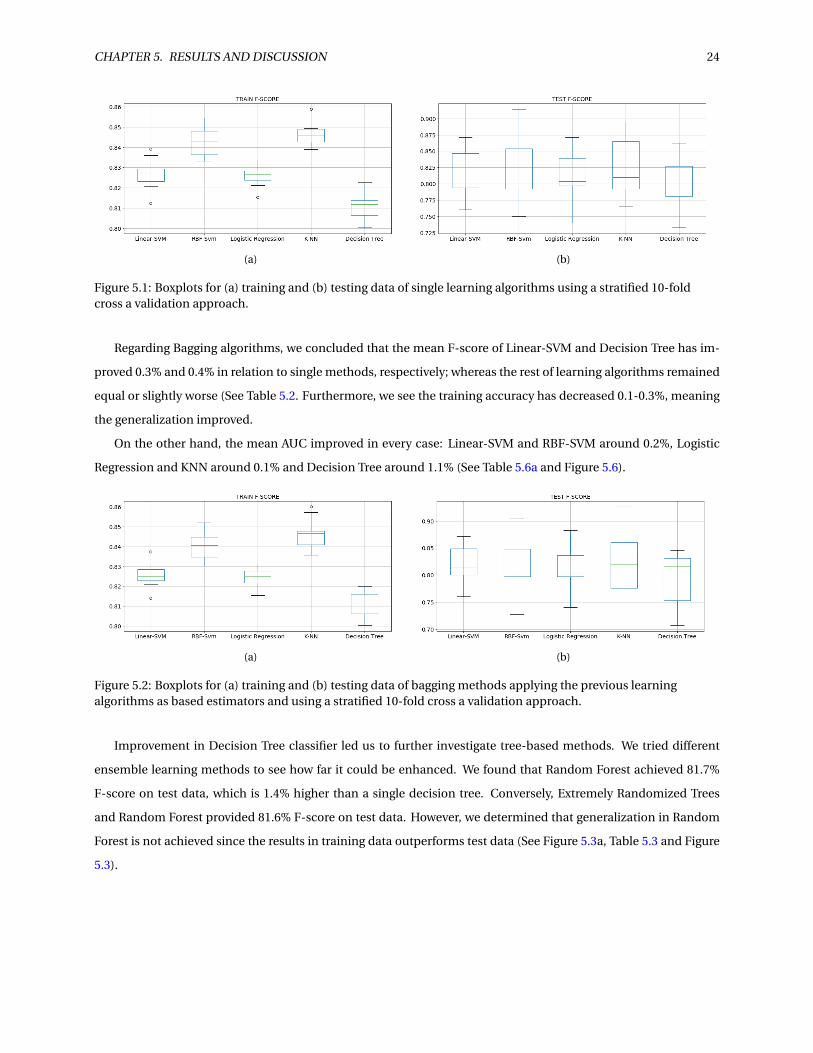
Figure 5.1: Boxplots for (a) training and (b) testing data of single learning algorithms using a stratified 10-foldcross a validation approach.

Regarding Bagging algorithms, we concluded that the mean F-score of Linear-SVM and Decision Tree has im-

proved 0.3% and 0.4% in relation to single methods, respectively; whereas the rest of learning algorithms remained

equal or slightly worse (See Table 5.2. Furthermore, we see the training accuracy has decreased 0.1-0.3%, meaning

the generalization improved.

On the other hand, the mean AUC improved in every case: Linear-SVM and RBF-SVM around 0.2%, Logistic

Regression and KNN around 0.1% and Decision Tree around 1.1% (See Table 5.6a and Figure 5.6).

(a) (b)

Figure 5.2: Boxplots for (a) training and (b) testing data of bagging methods applying the previous learningalgorithms as based estimators and using a stratified 10-fold cross a validation approach.

Improvement in Decision Tree classifier led us to further investigate tree-based methods. We tried different

ensemble learning methods to see how far it could be enhanced. We found that Random Forest achieved 81.7%

F-score on test data, which is 1.4% higher than a single decision tree. Conversely, Extremely Randomized Trees

and Random Forest provided 81.6% F-score on test data. However, we determined that generalization in Random

Forest is not achieved since the results in training data outperforms test data (See Figure 5.3a, Table 5.3 and Figure

5.3).


(a) (b)

Figure 5.3: Boxplots for (a) training and (b) testing data of tree-based learning algorithms using a stratified 10-foldcross a validation approach.

With regard to the AUC, it has improved around 1% in Random Forest and bagging trees, while Extremely Ran-

domized Trees goes further to 1.2% improvement regarding single decision trees (See Table 5.3 and Figure 5.7a).

Furthermore, we evaluated boosting methods, which decreases bias of the learning algorithms. We could ver-

ify that the XGBoost provides the best performance (82.1% mean F-score on test data) along with AdaBoost with

logistic regression as a weak learner. On the other hand, we concluded that these learning algorithms generalizes

less than the rest, since the F-score for training data is relatively higher than test data. (See Table 5.4 and see Figure

5.4). Regarding AUC, Voting Classifier shows the highest value along with XGBoost and Gradient Tree Boosting.

(a) (b)

Figure 5.4: Boxplots for (a) training and (b) testing data of Boosting methods and Voting classifier using a stratified10-fold cross a validation approach.

To conclude, we can claim almost all the classifiers considered in this project provide similar mean F-score

results. Random Forest presented a relatively high training mean F-score on test data, even though we tuned the

hyper-parameters. Nevertheless, SVM-RBF yields the best results in terms of mean F-score in relation to test and

training data, as well as AUC values.

CH

AP

TE

R5.

RE

SULT

SA

ND

DISC

USSIO

N26

Learningalgorithms

Trainingaccuracy

Testaccuracy

TrainingF-score

TestF-score

Trainingprecision

Testprecision

Trainingsensitivity

Testsensitivity

Linear - SVM 0.803±0.008 0.790±0.048 0.827±0.048 0.814±0.035 0.805±0.048 0.808±0.069 0.849±0.008 0.831±0.067RBF - SVM 0.819±0.008 0.799±0.060 0.843±0.007 0.825±0.047 0.810±0.006 0.804±0.072 0.879±0.009 0.855±0.066

Logistic Regression 0.803±0.006 0.789±0.052 0.826±0.005 0.813±0.040 0.809±0.006 0.810±0.074 0.843±0.005 0.827±0.075K-NN 0.825±0.007 0.797±0.059 0.846±0.006 0.824±0.042 0.821±0.008 0.807±0.078 0.873±0.006 0.853±0.078

Decision Tree 0.782±0.007 0.763±0.051 0.806±0.008 0.789±0.048 0.797±0.025 0.782±0.061 0.817±0.042 0.802±0.075

Table 5.1: Evaluation metrics (mean ± std) for test and training data of single learning algorithms using a stratified 10-fold cross a validation approach.

Learningbase

algorithms

Trainingaccuracy

Testaccuracy

TrainingF-score

TestF-score

Trainingprecision

Testprecision

Trainingsensitivity

Testsensitivity

Linear - SVM 0.803±0.007 0.793±0.048 0.826±0.048 0.817±0.035 0.808±0.008 0.814±0.07 0.844±0.005 0.829±0.064RBF - SVM 0.818±0.008 0.794±0.059 0.840±0.007 0.819±0.048 0.814±0.008 0.807±0.072 0.869±0.069 0.839±0.071

Logistic Regression 0.802±0.005 0.789±0.053 0.825±0.005 0.813±0.040 0.808±0.006 0.810±0.074 0.842±0.005 0.827±0.077K-NN 0.822±0.007 0.793±0.070 0.846±0.007 0.824±0.051 0.808±0.009 0.795±0.08 0.888±0.01 0.867±0.087

Decision Tree 0.790±0.007 0.770±0.050 0.811±0.006 0.793±0.047 0.810±0.01 0.797±0.061 0.812±0.013 0.841±0.080

Table 5.2: Evaluation metrics (mean ± std) for test and training data of bagging methods applying the previous learning algorithms as based estimators andusing a stratified 10-fold cross validation approach.

Learningalgorithms

Trainingaccuracy

Testaccuracy

TrainingF-score

TestF-score

Trainingprecision

Testprecision

Trainingsensitivity

Testsensitivity

Random Forest 0.895±0.005 0.799±0.054 0.908±0.041 0.817±0.047 0.881±0.005 0.803±0.072 0.938±0.006 0.841±0.081Extremely

Randomized Trees0.850±0.009 0.786±0.058 0.870±0.008 0.816±0.042 0.836±0.007 0.791±0.074 0.908±0.01 0.850±0.061

Table 5.3: Evaluation metrics (mean ± std) for test and training data of ensemble tree-based learning algorithms using a stratified 10-fold cross a validationapproach.

CH

AP

TE

R5.

RE

SULT

SA

ND

DISC

USSIO

N27

Learningalgorithms

Trainingaccuracy

Testaccuracy

TrainingF-score

TestF-score

Trainingprecision

Testprecision

Trainingsensitivity

Testsensitivity

AdaBoost - DT 0.802±0.008 0.781±0.048 0.823±0.008 0.805±0.038 0.811±0.01 0.803±0.060 0.836±0.017 0.810±0.040AdaBoost - LR 0.804±0.006 0.792±0.051 0.824±0.005 0.814±0.042 0.819±0.008 0.819±0.075 0.829±0.005 0.821±0.091

Gradient Tree Boosting 0.812±0.009 0.792±0.065 0.835±0.008 0.818±0.049 0.812±0.011 0.807±0.079 0.859±0.010 0.839±0.069XGBoost 0.827±0.006 0.796±0.063 0.849±0.006 0.821±0.048 0.826±0.006 0.812±0.079 0.873±0.01 0.839±0.072

Table 5.4: Evaluation metrics (mean ± std) for test and training data of boosting learning algorithms using a stratified 10-fold cross a validation approach.

Learningalgorithms

Trainingaccuracy

Testaccuracy

TrainingF-score

TestF-score

Trainingprecision

Testprecision

Trainingsensitivity

Testsensitivity

Voting Classifier 0.828±0.006 0.798±0.055 0.849±0.005 0.823±0.042 0.824±0.005 0.808±0.073 0.876±0.006 0.847±0.0623

Table 5.5: Evaluation metrics (mean ± std) for test and training data of a soft voting classifier of single learning algorithms mentioned previously in Table 5.1using a stratified 10-fold cross a validation approach.


Learningalgorithms

AUC

Linear - SVM 0.875±0.056RBF -SVM 0.876±0.058

Logistic Regression 0.873±0.056K-NN 0.872±0.057

Decision Tree 0.860±0.062

(a)

Learningbase

algorithmsAUC

Linear - SVM 0.877±0.055RBF -SVM 0.878±0.056

Logistic Regression 0.874±0.058K-NN 0.873±0.058

Decision Tree 0.871±0.056

(b)

Table 5.6: Area Under the Curve (AUC) (mean ± std) for test data of (a) single learning algorithms and (b) baggingmethods applying the previous learning algorithms as based estimators using a stratified 10-fold cross a validationapproach.

Learningalgorithms

AUC

Decision Tree 0.854±0.060Random Forest 0.864±0.062

Extremely Randomized Trees 0.866±0.059Bagging Decision Tree 0.864±0.057

(a)

Learningalgorithms

AUC

AdaBoost - DT 0.863±0.0540AdaBoost - LR 0.868±0.0534

Gradient Tree Boosting 0.8705±0.0559XGBoosting 0.8703±0.0561

Voting Classifier 0.8711±0.056

(b)

Table 5.7: Area Under the Curve (AUC) (mean ± std) for test data of (a) decision tree and ensemble tree-basedlearning algorithms and (b) boosting and voting methods applying the previous learning algorithms as basedestimators using a stratified 10-fold cross a validation approach.

(a) (b)

Figure 5.5: ROC for test data of (a) single learning algorithms and (b) bagging methods applying the previouslearning algorithms as based estimators using a stratified 10-fold cross a validation approach.


(a) (b)

Figure 5.6: ROC for test data of (a) Tree-based methods and (b) Boosting methods and voting classifier applyingthe previous learning algorithms as based estimators using a stratified 10-fold cross a validation approach.

5.2 Comparison with previous research

Owing to the world-wide increasing mortality of cardiovascular disease each year and the resulting cost require-

ments, many researchers have applied data mining approaches in the diagnosis of heart disease.

In particular, the so-called Cleveland dataset has been used several times due to its powerful information. De-

spite this fact, we have pre-processed the data. In this study, we found many difficulties addressing this stage.

Firstly, the dataset was imbalanced, which is where there are more instances from one class than the other. Sec-

ondly, there is missing data, and thirdly, it contains a mix of data types (categorical and continuous).

The studies found in the literature were very unclear about the pre-processing of the data [10] [11]. A few of

them discarded those instances which contained any single missing sample [12]. Others, just contemplated the

Cleveland data source and discarded the remaining (Hungary, Switzerland, and VA Long Beach). Various research

studies include categorical data with an unclear form of data transformation. On top of that, most of those studies

did not use a cross-validation approach to evaluate their models and they used accuracy instead of F-score as the

most important metric unit. We found one research project [13] which uses a cross-validation strategy, providing

a 48.53% precision with a Naïve Bayes algorithm. Even though this study used cross validation, it used a model

which assumed the features involved are independent from each other. In our view, such assumption cannot be

made due to some features are somewhat correlated and not completely independent from each other.

The highest accuracy was found by Anbarasi, et al [14] with a value of 99.2% using a genetic algorithm with

Decision Tree. However, the study did not use any cross-validation approach nor determined the generalization

nature of the model.


This project offers a complete Knowledge Discovery and Data-mining approach, including an exhaustive data

pre-processing, performing MICE imputation and variable transformation with features selection. We then pro-

vided an outright Exploratory Data Analysis, where we showed the distributions of the features. Finally, we tuned

the hyper-parameters and evaluated our models adopting a stratified 10-fold cross-validation approach. The re-

sults are then compared using F-score and AUC due to the imbalanced nature of our dataset, the accuracy metric

was not utilized (see Apendix-A).

Chapter 6

Conclusions and Future Work

In this final chapter, we presented the obtained conclusions. We then illustrated the potential benefits which

can be derived in the health scope. Finally, we described the possible future work which could be developed re-

garding this project topic. As such, we determined how much research remains to be done.

6.1 Conclusions

Nowadays, CAD plays an important role in a clinical and economic context. There is a high percentage of

prevalence among mid-aged people. Furthermore, treatment and control of this particular disease can be expen-

sive. Thus, we aim to provide a tool which can improve the application of available resources regarding this spe-

cific chronic condition. For that purpose, we analyzed demographic and clinical data from the so-called Cleveland

dataset and performed an exhaustive KDD approach which can derive whether a patient suffers heart disease.

Firstly, a pre-processing of this dataset was required due to its inconsistencies. We tried to have the most com-

plete and unbiased dataset. As such, we used MICE imputation. After that, we chose the most important attributes

by means of various feature selection approaches. In addition to the target feature (diagnosis of heart disease), we

extracted the most important attributes using feature engineering. Finally, we transformed these features into a

suitable format that fits the proposed learning algorithms.

Secondly, we performed an exploratory data analysis: the number of male patients is far more higher than

female patients. Furthermore, female patients suffer heart disease at an elderly age, along with a higher level of

cholesterol, maximum heart rate achieved and ST-depression than male patients. Patients with atypical angina are

more likely to be at an elderly age, at a slightly higher level of cholesterol and heart rate achieved than asymptotic

chest pain patients. Moreover, we revealed that those patients with exercise induced angina contains lower values

of maximum heart rate achieved than those who do not experience it.

On the other hand, we could verify that patients who experienced exercise induced angina and asymptomatic

chest pain were more prone to be diagnosed with heart disease.

Eventually, we validated our models adopting a stratified 10-fold cross-validation and showing the ROC, AUC

31

CHAPTER 6. CONCLUSIONS AND FUTURE WORK 32

and mean ± std F-score. We verified that our models (single and ensemble) provide an average of 78-83% F-score

over the folds, and a mean AUC of 85-88%. The highest score is given by Radial Basis Function Kernel Support Vector

Machines (RBF-SVM), achieving 82.5% ± 4.7% and 87.6% ± 5.8% of F-score and AUC, respectively. Conversely, we

found that XGBoost and Random forest did not generalize well (overfitting) as the training F-score is relatively

higher than the test F-score.

In conclusion, we determined that data mining techniques offer other options to physicians to facilitate their

interpretations about diagnosis of heart disease considering clinical and demographic characteristics of patients.

6.2 Future Work

CAD has raised concern due to its relevance as a major cause of death. Statistical analysis and data mining

approaches could support physicians for disease treatment. As such, we present the potential work which remains

to be developed and advanced:

• The dataset dates from the 80’s. Currently, the most relevant characteristics to diagnose heart disease may

have changed since that time. Thus, we propose another study considering current data.

• We had some difficulties applying data-mining techniques to incomplete data. Therefore, another analysis

with only male patients suffering heart disease would be interesting (as those patients had the most complete

information).

• Gathering more data. The number of patients considered in this study (920) does not contain a fair popu-

lation representation. Moreover, those patients presented missing data. A higher number of complete data

examples will add more information to this research and will reduce the generalization problem.

• Performing other ML algorithms such as Neural Networks and some other ensemble methods (Stacking).

• Including data from various geographic location. Probably there are different patterns considering different

data from different places. Diet and lifestyle would differ from one place to another, and thus the character-

istics of patients.

Appendix A

State-of-the-art

In this Appendix, we explained the relevance of cardiovascular diseases, the influence of technology in clinical

decision support and the importance which data is having in real world applications. Later, we described what

some types of Data Mining and Machine Learning techniques which we evaluated in this project. Finally, we illus-

trated the ethics involved using this technique and the evaluation metrics we used to evaluate the performance of

the models involved.

A.1 Cardiovascular Diseases

Cardiovascular diseases (CVD) comprises of a wide range of medical issues of the circulatory system i.e., the

heart, blood vessels and arteries. Some of the most common diseases within this group include ischaemic heart

disease (heart attacks) and cerebrovascular diseases. Even though there is a small reduction of these problems

nowadays, it is still the major cause of death in the EU (See Figure A.1).

People suffering these issues face disability, reduced quality of life and, in some cases, premature death. In-

terventions towards lifestyle aims to reduce the prevalence of these diseases. The amount can be reduced by: the

avoidance of tobacco, at least 30 min/day of physical activity, eating healthy food, avoidance of weight gain and

maintenance of blood pressure below 140/90 mmHg among other factors [3].

In Sweden, CVD is also the major cause of death. Table A.1 shows the length of stay per 100K inhabitants,

the number of admissions per 100K inhabitants, the average length of stay, and the number of patients per 100K

inhabitants. In this table you can see men are more prone to be diagnosed with CVD than women. However,

according to Eurostate, death rates are much higher for women than for men. Moreover, according to Table A.2

the majority of the population aged older than 65 years old contains the highest prevalence of conditions from the

circulatory system.

In recent years, there has been a reduction of the number of deaths related to cardiovascular diseases due to the

discovery and adoption of new technologies such as screening, new ways to undergo surgical procedures as well

as the introduction of medication e.g., statins. There is also a change in the lifestyle of people e.g., less smokers.

33

APPENDIX A. STATE-OF-THE-ART 34

Figure A.1: Causes of death - diseases of the circulatory system in 2014. Extracted from Eurostat [3].

However, it is still the major cause of death and it is taking many lives over the years [3].

Regarding the healthcare personnel, there are between 5 and 20 cardiologist across almost every country from

the EU, with the number increasing every year. This suggests there is a concern about issues with the circulatory

system in the EU [3].

Measure Sex 2013 2014 2015 2016Men 13,882.36 13,528.12 12,817.05 12,105.83

Woman 11,435.02 11,160.15 10,494.56 9,696.34Length of stay per 100,000 inhabitantsBoth sexes 12,656.13 12,342.97 11,656.28 10,903.67

Men 2,674.04 2,583.98 2,486.47 2,385.73Woman 2,003.70 1,924.76 1,845.30 1,728.75Number of admissions per 100,000 inhabitants

Both sexes 2,338.17 2,254.05 2,166.02 2,057.94Men 5.19 5.24 5.15 5.07

Woman 5.71 5.80 5.69 5.61Average length of stayBoth sexes 5.41 5.48 5.38 5.30

Men 1,692.31 1,647.47 1,598.70 1,535.83Woman 1,331.64 1,284.16 1,238.88 1,173.44Number of patients per 100,000 inhabitants

Both sexes 1,511.60 1,465.64 1,418.86 1,355.02

Table A.1: Diagnoses of circulatory system problems in the Swedish In-Patient Care. Age: 0-85+. Statistics taken from The Healthand Welfare Statistical Database of Sweden [15].


Measure Sex 2013 2014 2015 2016Men 60,005.52 57,620.33 54,194.81 50,880.36

Woman 46,712.36 45,112.03 41,887.44 38,532.24Length of stay per 100,000 inhabitantsBoth sexes 52,764.85 50,832.97 47,539.05 44,222.65

Men 10,895.95 10,403.94 9,982.16 9,539.22Woman 7,871.80 7,504.07 7,168.67 6,683.24Number of admissions per 100,000 inhabitants

Both sexes 9,248.72 8,830.38 8,460.64 7,999.37Men 5.51 5.54 5.43 5.33

Woman 5.93 6.01 5.84 5.77Average length of stayBoth sexes 5.71 5.76 5.62 5.53

Men 6,864.53 6,601.00 6,386.39 6,105.48Woman 5,206.62 4,976.48 4,786.24 4,524.37Number of patients per 100,000 inhabitants

Both sexes 5,961.48 5,719.49 5,521.03 5,253.00

Table A.2: Diagnoses of circulatory system problems in the Swedish In-Patient Care. Age: 65+. Statistics taken from The Health andWelfare Statistical Database of Sweden [15].

A.2 Clinical Decision Support

Services provided at fast pace are believed to give user’s satisfaction. For example, considering a single medical

appointment: it is claimed a considerable amount of time is wasted when a patient is given "hands-on" treatment

i.e., vital signs, discussing with the physician and undergoing the procedure. Furthermore, there is also wasted

time when the patient is waiting for something to happen. However, healthcare service delivery is a very complex

procedure since each patient has a unique process to go through e.g., physical examination, lab analysis, imaging,

etc. [16] [17] [18].

Increasing quality of care, improving healthcare outcomes, avoiding adverse events or producing mistakes and

improving efficiency, cost-benefit and patient/provider satisfaction involves new ways to address these challenges.

Clinical decision support (CDS) provides assistance to physicians, patients, healthcare providers and related,

improving and enhancing healthcare delivery [19][20]. CDS has been claimed as a very useful tool to improve

healthcare quality [21].

There are mainly four different features to achieve this: i) add decision support to clinician’s plan, ii) bring

decision support at the time and location of the made decision, iii) provide suggestions of actions and iv) using a

computer/electronic device as the means to get decision support [22]. Automatically providing decision support

to physicians, eliminates the time physicians need to spend to look at suggestions of the system.

Furthermore, CDS improves consistency, robustness and reliability by using computers or electronic medical

devices by minimizing costs in terms of time and errors prone to manual entry abstractions. Thus, using CDS is

essential to improve quality-care since it decreases time, initiative and endeavor needed by clinicians to draw and

move towards system recommendations [22].


A.2.1 Telehealth

Using electronic services to support clinical decisions such as monitoring, patient-care and education [23]

helps to reduce costs and improve healthcare quality in effective, efficient, timely, safe, equitable and patient-

centered conditions [24][25][26]. To achieve these targets, integration of telehealth into traditional practises should

be accomplished.

Over the last decades, technology innovation has had a great impact in the population improving approaches

to consumers. Think about automated teller machines (ATM), drive-through windows and self-service gas stations

[27] and recently the supermarket with free-checkout which Amazon just released at the beginning of 2018 [28].

Telehealth approaches includes home-based management for different diseases such as diabetes, hyperten-

sion or heart failure, reducing time for physicians visitations [29]. For example, taking the medical appointment

described in the above section, using a digital solution could assist the system to make the right priorities and save

time of the patient and practitioners.

On the other hand, healthcare is converging towards self-service: home-pregnancy tests, diabetes monitoring

for glucose, self-titrated insulin doses are a just a few examples of e-Health devices. The possibilities are infinite

(See Figure A.2). However, healthcare requires to be a synchronous and local service. This means the patient and

providers must be at the same time and place.

Figure A.2: Application of telehealth for monitoring health status or improving health outcomes. Extracted from[30].

Additionally, providers are facing different challenges: time-spending with patients, decision-making auton-

omy and managing the growth of information available. Electronic Health Records (EHR) is a tool which provides


reliable access from trusted sources, and helps the practitioners by decision support functions. As such, traditional

face-to-face encounters should be viewed in other way.

Approaches providing structural and organizational information management also helps practitioners to ad-

dress these challenges. Scheduling, checking out, hospital admissions and follow-up are some examples [31]. Some

of the above mentioned examples are used nowadays: practitioners and patients share e-mails and SMS to provide

health-care delivery. Digital health is a promising solution to address these challenges.

To conclude, telehealth should respect and respond to patient needs and characteristics. Nowadays, many

organizations allows the visualization of medical results, notes or patients records with other patients in a secure

and safe way. Limitations when it comes to clinical visitations due to limited mobility or distant location of medical

care centres should be addressed by virtual encounters which could improve compliance with more CDS [32].

A.2.2 Predictive Analytics

Satisfying patient’s involvements, reducing healthcare cost and improving heathcare results are believed to be

accomplished by the use of predictive analytics. Using medical devices, wearable technologies, data acquisition

by means of electronic data repositories such as EHRs and different risk-model prediction helps to improve the

current growth healthcare service which has been developed nowadays [33][34][35]. However, we also need to

ensure a private and safe procedure to deal with patient’s data. We will come to this later in the next sections.

Additionally, the vast amount of clinical, behavioural, biological data which is continuously generated from

patients can be essential to determine new patterns of knowledge which meets the needs of patients, physicians,

healthcare providers, and health policy makers.

Nowadays, there is no straight path for how to use the increasing information accessible in an efficient fashion.

Decision making needs crucially enhanced personalized predictions about prognosis and treatment delivery, ap-

proaches regarding safety issues with drugs and devices, and better prevention, diagnosis and treatment methods

by taking advantage of the data that is ready to use [36].

Clinical research and practice move towards cultivating new knowledge due to the complexity of real-world

targets. This is why the healthcare activities need data analytics to speed up the process of getting new knowledge

and reducing time and cost for new research [37].

Achievement of medical knowledge traditionally involved inception from empirical approaches based on pre-

vious experiments and theory. Nonetheless, exploiting data signify addressed issues could be solved without un-

derstanding direct causes of that particular research question. For instance, finding new patterns of patient groups

might imply new distributions according to a wide scope of patient characteristics [38]. Meaning that, this acquired

knowledge can be used to determine enhanced mechanisms to build better treatments and response to patients

needs, in the same way Amazon is suggesting to their customers their preferences without knowing those particular

customers have them.

Data mining and Machine learning (ML) techniques handle advanced analytic and computational systems to

acquire knowledge from the data, aiming to predict and discover new patterns [36]. These techniques commonly


involve hypothesis testing and statistical methods. The healthcare environment pursues to be a learning service.

Other fields such as astronomy are getting very valuable outcomes by using these kind of techniques [39]. One of

the many advantages of using ML methods is the confirmation bias elimination which usually contaminates the

research, since the personnel who take over the methodology do not have prior knowledge of what would be the

results. However, it is true that expertise is relevant to assess and interpret new findings.

Therefore, the target is to develop statistical and mathematical algorithms which can understand many factors

related to biological, clinical, demographic and psychological characteristics of patients, as well as practitioners,

physicians, geographical and hospital features from data of healthcare encounters, electronic medical devices and

administrative assertions increasingly available [36]. For example, some research evaluate the performance of ML

techniques [40][41]. These studies revealed some clusters of phenotype hospitals.

A.3 Data Mining and Machine Learning

As commented in the previous sections, the continuous growth of available information leads to discovery of

hidden potential useful knowledge. In the field of data mining, the data is electronically stored and then automated

by a computer. This field seeks to find new patterns that can be automatically acquired, validated and applied for

predictions by analyzing data already present in data repositories. Even though a clear definition of data mining

has never been built, often data mining is just one step within the large process of knowledge discovery and Data

mining (KDD) [42] (See Figure A.3).

Figure A.3: Typical steps of KDD. Extracted from [43].

Data mining methods are related with fields such as Artificial Intelligence (AI) and (ML). Actually, data mining

and ML are sub-fields of AI, and ML techniques are shared with data mining approaches. On one hand, data mining

aims to find patterns that hold in the set of samples (usually stored in a data repository) which is also expected to

hold in other data not stored in that repository, thus the objective is to give a comprehensible description of these

patterns.


On the other hand, ML samples are based on experience. It aims to find patterns that may be used for future

applications [44].

Some challenging data mining applications are related to bioinformatics, biomedical applications, protein data

analysis, bio-medicine, fraud detection, financial engineering, modelling and control in process chemical indus-

tries and decision making in overall terms [43][45][46][47][48].

According to Tom Mitchell [44], we can claim an algorithm is learning if it has the capacity to improve performance.

We can define learning behaviour in a more formal way:

Given a task T, a performance criterion C, and experience E, a system learns from E, if it becomes better at solving

a task T, as measured by criterion C, by exploiting the information in E.

On the other hand, learning can be classified as supervised, when a function f : X → Y predicts the value of

some target attributed Y from other values X . This function is learned from examples of the form (x, y), where

y = f (x). When the y values are not given, then we get an unsupervised learning setting.

Another setting which is in between both supervised and unsupervised, is called semi-supervised learning. This

setting contains just a few values of the y values. One may think whether such unlabeled examples are useful at

all. Actually, the unlabeled example provides more information about the distribution of the whole set of examples

[49].

Figure A.4: Example of semi-supervised learning. Blue crosses are the labelled examples, while u-shapes areunlabeled examples. Extracted from [50].

According to Figure A.6, we can see how the unlabelled examples helps to define the boundaries of classifica-

tion. If unlabelled examples were not considered, it might lead to a negative generalization i.e., misclassification

for new predicted instances [50]. Therefore just a few labels are needed to build a relatively good predictive model.

Prediction learning commonly explains a learned model which predicts, for a given object, the value At of one

specific attribute from values of all other attributes. In other words, a function can be defined as f : A1 × A2 × A3 ×...× AD−1 → AD where t = D and A1 × A2 × A3 × ...× AD−1 and Y = AD . When the target takes values from an mixed


set of values (e.g., red, green, blue) it is called nominal, while the target takes values from a complete ordered set

(e.g., small, medium, large) it is called ordinal. On the other hand, if a variable takes values from real numbers it

is called numerical. Learning a model for predicting, when its target value is continuous and numerical, is called

regression. Additionally, if the target value is nominal and discrete, then it is called classification [44].

A.3.1 Model Validation

The selection of our approaches is based on the nature of the problem, the assumptions we make about data

and the results that we obtain with a test or validation dataset.

In order to assess our models, we normally split our dataset into a training/test set. However, when the dataset is

imbalanced and we do not have enough samples there are other options we can consider such as cross-validation.

A.3.2 Cross validation in Machine Learning

As commented above, there is a need to validate the stability of our estimators. We need to make sure our

models have got the majority of the patterns from the data correctly, and this comes from not collecting too much

noise (low on bias and variance).

The general problem comes from the following question: How well the learning algorithm will perform on an

independent/unseen dataset. Towards this end, cross-validation comes into play. This method provides ample

data for training the model and also leaves ample data for validation.

In K-fold cross validation, the data is divided into K subsets. The holdout method is repeated K times, such

that each time, one of the subsets is used as the test set/validation set and the remaining K-1 subsets are held in a

training set. The error is estimated by averaging over all K trials to get total effectiveness of the model. As such, we

can assure that every data point gets to be in a validation set exactly once, and gets to be in a training set k-1 times.

This significantly reduces bias as we are using most of the data for fitting. Additionally, it certainly reduces variance

as most of the data is also being used in validation set.

Figure A.5: Example of 10-Fold Cross-Validation strategy to evaluate machine learning algorithms.

In some cases, the data suffers a large imbalance in the response variables, there is then a slight variation in


the previous approach that will overcome with the issue. In this technique, called Stratified K-fold validation, each

fold tries to get the same percentage of samples of each target class as the complete set, the mean response value

is approximately equal in all the folds.

A.3.3 Bias Variance trade-off

After fitting a model, problems arise when determining its performance. As stated above, from a practical point

of view we can use a training and test or validation set to verify the quality of our models and avoid strong fit on

the training set. From a theoretical point of view, we can illustrate how a complex model can produce overfitting.

Assuming we have a functional relation Y = f (X )+ ε where ε is the error estimation with E(ε) = 0 and V ar (ε) =si g ma2. Then, the prediction error at x can be expressed for f̂k , an approximation to f , as:

EPEk (x) = E [(Y − f̂k (x))2|X = x] = si g ma2 + [Bi as2( f̂ (x))+V ar ( f̂k (x))] (A.1)

Bi as f ( f̂ ) = E [ f̂ − f ],V ar f ( f̂ ) = E [( f̂ −E [ f̂ ])2] (A.2)

From the previous equations Bi as f ( f̂ ) and V ar f ( f̂ ) sum the Mean Square Error (MSE), and in addition to

EPEk (x) depend on our model.

As a general result, when the complexity of the model grows the plain error (bias) decreases but the noise (vari-

ance) increases.

Figure A.6: Trade-off between bias and variance. Extracted from [51].


A.3.4 Previous research - predictive analytics

These types of data have been used in the medical scope. Data from the health electronic records (EHR) seem

to be promising to build and improve a sustainable healthcare system. Clinical data such as blood tests, lab re-

sults, diagnoses and procedures comprise of numerical and categorical data, as well as demographic data such as

age, sex, or ethnicity forming, in turn, heterogeneous data. Some studies have used this information for statistical

analysis and predictive analytics [52] from EHR of a university hospital in Madrid considering International Classi-

fication Diseases (ICD) codes as well as demographic data. Other study identified acute ischemic strokes by using

ICD codes and machine learning models such as classification and regression tree (CART) and logistic regression

[53].

Other studies used free-text in EHR which comprises a huge amount of clinical information about health state

and patient history. Using Support Vector Feature Selection for early detection of anastomosis leakage were proved

to develop prediction models that could support physicians and patients during preoperative decision making

phases [54].

Furthermore, predicting colorectal surgical complications using heterogeneous clinical data succeeded to be

used as a framework for preoperative clinical decision support. This study exploited heterogeneous data from

multiple sources comprising free text, blood tests and vital signs (temperature, pulse and blood pressure) using

linear and non-linear Support Vector Machines [55].

Owing to the world-wide increasing mortality in cardiovascular diseases and the current availability of EHR,

there has been some studies which had used data mining techniques to extract hidden information providing help

to physicians to diagnose heart diseases [56] [11] [13] [57] [58] [59]. These research projects used techniques such

as decision trees, Naive Bayes, neural networks and support vector machines, among others.

Diagnosing these type of conditions has never been an easy task. In fact, heart diseases may have symptoms

which are not clearly described as well as the manifestation of pathological and functional symptoms which are

related to other organs. Using data mining techniques could reduce the diagnosis time and improving of the ac-

curacy since the diagnoses is relied on the practitioner experience and sometimes, there would be other reasons

behind the scene.

Logistic Regression

Even though Logistic regression suggests to perform some kind of regression, it is a linear model for classifica-

tion. In the literature is sometimes called logit regression, maximum-entropy classification or the log-linear clas-

sifier. The possible outcomes are taken from probabilities of a single trial using a logistical function (See Equation

A.3 and Figure A.7):

f (x) = L

1+e−k(x−x0)(A.3)

where:


e = natural logarithm base

x0 = the x-value

k = the steepness of the curve

L = the curve’s maximum value

Figure A.7: Standard Logistic sigmoid function i..e, L=1, k=1, x0=0.

There has been some research studies in the healthcare scope, using logistic regression analysis for the early

stage of epidemic of severe acute respiratory syndrome. These groups of researchers achieved a sensitivity and

specificity of 100% and 93%, respectively, in diagnosing of this disease. [60]. Furthermore, logistic regression was

used to differentiate between benign and malignant lesions accomplishing a diagnostic accuracy of 0.8 ± 0.07 [61].

Decision Trees classification

This popular method combines good predictive accuracy with high interpretability and efficient learning and

prediction procedures. A decision-tree can be illustrated as a tree-shaped structure representing an input X to

some output Y . The node at the top is called root, whereas the nodes which have outgoing edges are called internal

nodes, and those which have not got incoming edges are called leaves.

Figure A.8: Example of a decision tree describing whether or not playing tennis considering climatologicalconditions.

The procedure consisting in map any x ∈ X to a single y ∈ Y is as follows: Starting with the root node of the

tree, we construct a path from the root to a leaf by computing in each node the outcome of its associated test for x,

and following the outgoing edge which is labelled with that outcome until a leaf is reached. The value to which x is

mapped by the tree is then the value y stored in that leaf [62][44] .


On the other hand, some problems arise whilst splitting. Even though the decision tree seems to perform re-

markably well when evaluated on training data, it performs not as well on the instance space. This is called over-

fitting. To solve this, among other approaches, there is one bagging estimator called random forest. To control

overfitting and improve accuracy, this estimator fits several decision trees on various subsamples of the dataset

and averages the result. [63] [64].

Instance-based learning: K-Nearest Neighbors (K-NN)

The basic idea of Instance-based learning is there is no-learning. The hypothesis learned is the dataset itself.

That is, if an instance contains the same properties as the new instance, it is likely that the target values are also the

same.

Figure A.9: Example of 3-NN. In this case the new instance got 2 white neighbors and 1 black neighbor, thus it willbe classified as white.

The nearest neighbor algorithm works as follows: looking at the instances previously seen, classify the new

instance according to the similarity to the instances you have seen before. If it is similar enough to the old instances,

then assign the same class to the new instance. Based on that, a more robust method called k-NN was constructed.

Intuitively, for some value k ∈R, take the k nearest neighbors of the new instance, and match the class that is more

similar among these k neighbors (See Figure A.9) [65][66]. Similarity is usually evaluated as euclidean distance:

d(p, q) =√

(q1 −p1)2 + (q2 −p2)2 +·· ·+ (qn −pn)2 =

=√

n∑i=1

(qi −pi )2(A.4)

with p and q being the points measured.

This methods works surprisingly well in some cases, and terribly in others. k-NN method is optimized by dif-

ferent approaches like weighting the examples or using prototypes [67].

Some studies worked with the early detection of melanoma from benign and skin lesions based on images

obtained from epiluminiscense microscopy. They achieved an average specifity of 79% and a sensitivity of 98%,

concluding that this would reduce unnecessary surgery since the improved accuracy of diagnosis [68].


Support Vector Machines (SVM)

In general, the parameters (e.g. number of hidden neurons) searching domain in artificial neural networks

(ANN) contains multiple local minima. The underlying reason is the techniques used, which increase the general-

ization problem. Lately, a technique called Support Vector Machines (SVM) sheds a new light, aiming to undertake

these problems. SVM is based on kernel functions such as linear, polynomial, splines and radial based functions

(RBF). These consist in projecting the observed domain data into another domain of higher dimension where a

classificatory divisor is built up (hyperplane). This hyperplane minimizes misclassification subjected to maximiz-

ing the minimum distance (margin) between the hyperplane and any instance of the training set [69][70].

Therefore, SVM has two targets: i) Looking for a classificatory divisor i.e., hyperplane with the largest minimum

margin; ii) Looking for a classificatory divisor i.e., hyperplane that separates as many instances as possible.

Figure A.10: Illustration of a linear classification problem with linear separable data. (Left) infinite separatinghyperplanes; (Right) definition of unique hyperplane, maximizing distance of datapoints

Linear SVM can be used for separable and non-separable data points (the latter one shows up in most real-life

situations) using lagrangian multipliers and Karush-Kuhn-Tucker conditions. SVM can be expanded to the non-

linear case where kernels such as polynomial and RBF come into play [71].

On the other hand, optimization methods such as Least-Squares SVM (LS-SVM) have been studied and proved

to perform better than simple SVM due to its heavy computations when datasets become larger. Furthermore, tun-

ing of parameters used in LS-SVM can be approached by different methods such as cross-validation, bootstrapping,

Bayesian inference or application of generalization bounds [71].

Applications of SVM for prediction of diabetes and pre-diabetes has been studied. An alternative approach was

presented to detect persons with these common diseases. It achieved a considerable high prediction rate and thus

it is confirmed to be a valid approach for prediction of diabetes [72].

A.3.5 Bootstrap aggregating (bagging)

This ensemble strategy has come up to improve the stability and precision of other learning algorithms decreas-

ing both variance and overfitting.


Bagging methods use base estimators to build another estimator, inheriting some properties from the base

estimators and improving some weakness from them. The methodology uses some randomness, like bootstrap or

random split points, to build different estimators and reduce the dependence among them [73].

Different bagging methods use different strategies to compute the new predictors.

For instance, Random Forest uses bootstrapping and selects a random subset of available features at each split-

ting point for searching the best option. Others such as perfect Random Forest [74] selects randomly the variable

and splitting the point. For a classification problem, the bagging estimator returns the class with the majority of

the votes [73].

There is an interesting analogy with Condorcet’s jury theorem which perfectly illustrates why bagging algo-

rithms work: we know Modern human societies are complex social structures where people have financial and

social interactions. Our inherent purposes leads to maximize our utility and our profit, usually confronting other

humans. Consequently, political economics is at the heart of any modern society, pretending to substitute our

primitive war for resources for a new war of words for resources.

Over the last centuries, we have seen democracy has been crowned as the new state-of-the-art technology in

human organization. Simultaneously, the world has grown and improved as never before. Why is that so? Democ-

racy is a type of human bagging.

Assuming that a group of people should decide between two options, only one of them is correct and that each

voter has a probability greater than 0.5 of taking the correct option, then the aggregate result will converge to 1 as

the number of independent voters is increased [75] [76].

A.3.6 When does Bagging work well?

In bagging, each model is learned by the same learning system L, from resamplings Ti of one training set T.

Considering the case that all classifiers are exactly the same, one may think the models hi might be similar too. If

the differences on the training sets Ti are too small, they may be even equal, and thus the learner L will not produce

different models.

One can claim bagging works well if the learner L which is being used is an unstable learner. In that context,

a learner is believed to be unstable if small changes in the training set may give an increase to large differences in

the model learned. On the other hand, a stable learner will not be influenced that much by small changes in the

training set.

Decision trees are deemed to be unstable learners, and are considered as a good candidate for bagging methods.

A.3.7 Boosting methods

In this ensemble method, the aim is to reduce both bias and variance of learning predictors [77]. As in the

previously described approaches, boosting learners used base estimators to build another estimator, inheriting

some properties from the base estimator and improving some of its weaknesses.


These boosting methods focus mainly in the samples which have been incorrectly classified or estimated in the

previous steps. Some approaches deal with it differently: Gradient boosting uses the residual of each prediction

as a guide to orientate the growth of the following learner. On the other hand, AdaBoost fits a sequence of weak

predictors on slightly modified versions of the original data set.

The idea behind boosting is quite simple: once you know how to do something, focus on the fields where you

are not experienced. In contrast to bagging algorithms where we use weak learners to estimate the whole dataset,

boosting methods build a strong learner in a different part of the dataset, leaving each new weak learner focusing

on improving the previous elements with the bigger prediction error [51].

Previously, we compared bagging with a democracy. Now, we can compare boosting with a technocracy where

each expert (weak learner) from the government (strong learner) focuses on a concrete area for learning and ruling

purposes.

A.4 Ethics and datasets

Data privacy from patients and consent have become more sensitive over the last decades. How to manage it is

quite challenging for the population, especially when the amount of patients become larger where the data request

and consent gets complicated. Developers of predictive analytics should be aware that if they are allowed to use

patient data, provided that they accomplish certain regulations regarding privacy of healthcare data.

On the other hand, one may understand that all individuals involved in this use of data should be informed

properly.

A suggestion would be to notify them when visitation to the physician consultation occurs. The physician will

ask the patient whether he wants to provide his records for quality-improvement purposes.

Also, there is a concern regarding equitability. Performing statistical analysis considering different sex, races

and ethnicity is always a sensitive topic. Allowing care-delivery must be independent of these characteristics

[78][79].

Accomplishing the obtention of insights from large datasets is easier said than done. Privacy concerns make it

difficult for researchers to access real data. Creating synthetic data i.e., artificial data can avoid this fact as well as the

lack of access to real data. One should model an entire database, by sampling and recreating an artificial version

which looks very similar to the original dataset in statistical terms. This strategy has succeeded when assessing

artificial intelligence predictive methods. It suggests that synthetic data can replace real data causing researchers

to overcome the massive barrier to entry accessibility and to get rid of the "privacy bottleneck" [80].

To conclude, this area is changing continuously, the use of data should be constantly assessed, evaluated, up-

dated and re-implemented in ethics and private terms by developing strategies which could tackle all of these issues

[81].


A.5 Evaluation Metrics

The aim of classifiers is to map instances to classes, as one may consider which classifiers performs better in

terms of accuracy by applying a particular classification task. Assuming we are trying to detect if a patient has

cancer or not, there are 4 possible outcomes: (a) True positive (TP): when a patient has cancer and is diagnosed by

the classifier as cancer; (b) False Negative (FN): the patient has been diagnosed as healthy, but in reality has cancer;

(c) True Negative (TN): if the patient has been declared healthy and has no cancer; (d) False Positive (FP): if the

patient is diagnosed with cancer, and he is actually healthy. The confusion matrix shows this (See Table A.3).

Actual ClassPositive Negative

Testoutcomepositive

True Positive(TP)

False positive(FP, Type I error)

Precision#T P

#T P+#F P

Testoutcomenegative

False negative(FN, Type II error)

True negative(TN)

Negative predictive value#T N

#F N+#T N

Sensitivity#T P

#T P+#F N

Specificity#T N

#F P+#T N

Accuracy#T P+#T N#T OT AL

Table A.3: Confusion Matrix. It shows the rates of correct and incorrect classifications. Correct classifications areshown in green squares on the matrix diagonal, while incorrect classifications form the red squares. the idealscenario is that the red squares corresponds to small rates i.e., few misclassifications.

In the research, we have seen the accuracy term has been chosen to be the define metric to evaluate quality in

some of the models. However, this can be misleading. Assume we have a binary classification problem with 20%

of samples from having a disease and 80% healthy samples. If we try to predict healthy samples and the model has

an accuracy of 80% then it looks like we have a very high percentage of success. However, we are leaving those 20%

thinking they have a disease. This is not correct, due to the accuracy, as we can see in Table A.3 just focuses on True

Positive and True Negative, thus the accuracy is only reflecting the underlying class distribution. This is particularly

dangerous for those datasets with a large class imbalance.

We have some other metrics which can tackle these issues. The F-score considers both the precision and the

sensitivity of the test to compute the score. The F-score is the harmonic average of the precision and recall, where

an F1 score reaches its best value at 1 (perfect precision and recall) and worst at 0. F-score can be seen as:

F-score = 2 · pr eci si on · sensi t i vi t y

pr eci si on + sensi t i vi t y(A.5)

Another useful metric is the receiver operating characteristic (ROC) graph which could give us some insights

considering this previous mentioned concepts. It displays the true positive rate (sensitivity) in the ordinates axes

and the false positive rate in the abscissas axes i.e, 1- specificity. Therefore, the ROC evaluation metric shows

the trade-offs between benefits and costs, in other words, it depicts the compromise between detecting cancer

correctly and the false alarm respectively. Each classifier provides a part of TP and FP rates which corresponds to a

point in the ROC graph. Perfect classification corresponds to the point (0,1) i.e., 100%TP rate and 0% FP rate.


Figure A.11: ROC curve. Point A shows perfect classification, whereas the performance of C is more "conservative"than B since it makes positive predictions only with strong evidence. Point B is therefore more "liberal", since itmakes positive predictions with weak evidence.

We could consider a classifier to give better performance if it has higher TP rate and a lower false positive rate.

Therefore, the most "northwest" the point is located, the better is the classifier. The area under the ROC curve

(AUC) measures the accuracy of the classifier (See Figure A.11).

Appendix B

Gantt Diagram

50

AP

PE

ND

IXB

.G

AN

TT

DIA

GR

AM

51

B.1 Gantt Diagram

2018

January February March April May

15 22 29 5 12 19 26 5 12 19 26 2 9 16 23 30 7 14 21 28

Understanding the project topic

Writing the report

Data retrieving, cleaning and selection

Exploratory and descriptive analysis

Performing ML analyses

Verifying analyses results

Figure B.1: Gantt diagram of the project.

Bibliography

[1] Eurostat. Healthcare expenditure statistics. http://bit.ly/2jr3dvu [Accessed: 22/02/2018].

[2] Commision of the European communities. White paper: Together for health: A strategic approach for the eu

2008-2013. Technical report.

[3] Eurostat. Cardiovascular diseases statistics. http://bit.ly/2IDkA4O [Accessed: 21/03/2018].

[4] Leland Wilkinson. Classification and regression trees.

[5] James Bergstra and Yoshua Bengio. Random search for hyper-parameter optimization. Journal of Machine

Learning Research, 13(Feb):281–305, 2012.

[6] Leo Breiman. Random forests. Machine learning, 45(1):5–32, 2001.

[7] T Hastie, R Tibshirani, and J Friedman. The elements of statistical learning 2nd edition, 2009.

[8] Robert E Schapire. Explaining adaboost. In Empirical inference, pages 37–52. Springer, 2013.

[9] Tianqi Chen and Carlos Guestrin. Xgboost: A scalable tree boosting system. In Proceedings of the 22nd acm

sigkdd international conference on knowledge discovery and data mining, pages 785–794. ACM, 2016.

[10] Sellappan Palaniappan and Rafiah Awang. Intelligent heart disease prediction system using data mining tech-

niques. In Computer Systems and Applications, 2008. AICCSA 2008. IEEE/ACS International Conference on,

pages 108–115. IEEE, 2008.

[11] Plamena Andreeva. Data modelling and specific rule generation via data mining techniques. In International

Conference on Computer Systems and Technologies-CompSysTech, 2006.

[12] My Chau Tu, Dongil Shin, and Dongkyoo Shin. Effective diagnosis of heart disease through bagging approach.

In Biomedical Engineering and Informatics, 2009. BMEI’09. 2nd International Conference on, pages 1–4. IEEE,

2009.

[13] Asha Rajkumar and G Sophia Reena. Diagnosis of heart disease using datamining algorithm. Global journal

of computer science and technology, 10(10):38–43, 2010.

52

http://bit.ly/2jr3dvu

http://bit.ly/2IDkA4O

BIBLIOGRAPHY 53

[14] M Anbarasi, E Anupriya, and NCSN Iyengar. Enhanced prediction of heart disease with feature subset selec-

tion using genetic algorithm. International Journal of Engineering Science and Technology, 2(10):5370–5376,

2010.

[15] The Health and Welfare Statistical Database of Sweden. In-patient Care Diagnoses statistics. http://bit.ly/

2HSQPfa [Accessed: 21/03/2018].

[16] Cathy Schoen, Robin Osborn, Sabrina KH How, Michelle M Doty, and Jordon Peugh. In chronic condition:

experiences of patients with complex health care needs, in eight countries, 2008. Health affairs, 28(1):w1–

w16, 2009.

[17] John Toussaint. Writing the new playbook for us health care: lessons from wisconsin. Health Affairs,

28(5):1343–1350, 2009.

[18] Peter Vermeir, Dominique Vandijck, Sophie Degroote, Renaat Peleman, Rik Verhaeghe, Eric Mortier, Giorgio

Hallaert, Sabine Van Daele, Walter Buylaert, and Dirk Vogelaers. Communication in healthcare: a narrative

review of the literature and practical recommendations. International journal of clinical practice, 69(11):1257–

1267, 2015.

[19] David W Bates, Michael Cohen, Lucian L Leape, J Marc Overhage, M Michael Shabot, and Thomas Sheridan.

Reducing the frequency of errors in medicine using information technology. Journal of the American Medical

Informatics Association, 8(4):299–308, 2001.

[20] Jonathan M Teich and Maureen M Wrinn. Clinical decision support systems come of age. MD computing,

17(1):43–46, 2000.

[21] Ida Sim, Paul Gorman, Robert A Greenes, R Brian Haynes, Bonnie Kaplan, Harold Lehmann, and Paul C Tang.

Clinical decision support systems for the practice of evidence-based medicine. Journal of the American Medi-

cal Informatics Association, 8(6):527–534, 2001.

[22] Kensaku Kawamoto, Caitlin A Houlihan, E Andrew Balas, and David F Lobach. Improving clinical practice

using clinical decision support systems: a systematic review of trials to identify features critical to success.

Bmj, 330(7494):765, 2005.

[23] Tracy A Lustig et al. The role of telehealth in an evolving health care environment: workshop summary. National

Academies Press, 2012.

[24] Santosh Krishna, Suzanne Austin Boren, and E Andrew Balas. Healthcare via cell phones: a systematic review.

Telemedicine and e-Health, 15(3):231–240, 2009.

[25] Kevin Patrick, William G Griswold, Fred Raab, and Stephen S Intille. Health and the mobile phone. American

journal of preventive medicine, 35(2):177–181, 2008.

http://bit.ly/2HSQPfa

http://bit.ly/2HSQPfa

BIBLIOGRAPHY 54

[26] Michael E Porter. What is value in health care? New England Journal of Medicine, 363(26):2477–2481, 2010.

[27] CM Christensen, JH Grossman, and J Hwang. The innovator’s prescription: a disruptive solution for health

care (p. li, 441 pp.). 2009.

[28] L Grimmer. Amazon go launch paints a checkout-free shopping future. 2018.

[29] Rashid L Bashshur, Gary W Shannon, Elizabeth A Krupinski, Jim Grigsby, Joseph C Kvedar, Ronald S Weinstein,

Jay H Sanders, Karen S Rheuban, Thomas S Nesbitt, Dale C Alverson, et al. National telemedicine initiatives:

essential to healthcare reform. Telemedicine and e-Health, 15(6):600–610, 2009.

[30] Santosh Kumar, Wendy J Nilsen, Amy Abernethy, Audie Atienza, Kevin Patrick, Misha Pavel, William T Riley,

Albert Shar, Bonnie Spring, Donna Spruijt-Metz, et al. Mobile health technology evaluation: the mhealth

evidence workshop. American journal of preventive medicine, 45(2):228–236, 2013.

[31] Lee H Schwamm. Telehealth: seven strategies to successfully implement disruptive technology and transform

health care. Health Affairs, 33(2):200–206, 2014.

[32] E Ray Dorsey, Vinayak Venkataraman, Matthew J Grana, Michael T Bull, Benjamin P George, Cynthia M Boyd,

Christopher A Beck, Balaraman Rajan, Abraham Seidmann, and Kevin M Biglan. Randomized controlled clin-

ical trial of “virtual house calls” for parkinson disease. JAMA neurology, 70(5):565–570, 2013.

[33] Peter WF Wilson, Ralph B D’Agostino, Daniel Levy, Albert M Belanger, Halit Silbershatz, and William B Kannel.

Prediction of coronary heart disease using risk factor categories. Circulation, 97(18):1837–1847, 1998.

[34] Thomas J Wang, Joseph M Massaro, Daniel Levy, Ramachandran S Vasan, Philip A Wolf, Ralph B D’agostino,

Martin G Larson, William B Kannel, and Emelia J Benjamin. A risk score for predicting stroke or death in indi-

viduals with new-onset atrial fibrillation in the community: the framingham heart study. Jama, 290(8):1049–

1056, 2003.

[35] William A Knaus, Elizabeth A Draper, Douglas P Wagner, and Jack E Zimmerman. Apache ii: a severity of

disease classification system. Critical care medicine, 13(10):818–829, 1985.

[36] Harlan M Krumholz. Big data and new knowledge in medicine: the thinking, training, and tools needed for a

learning health system. Health Affairs, 33(7):1163–1170, 2014.

[37] Asefeh Heiat, Cary P Gross, and Harlan M Krumholz. Representation of the elderly, women, and minorities in

heart failure clinical trials. Archives of internal medicine, 162(15), 2002.

[38] National Research Council et al. Toward precision medicine: building a knowledge network for biomedical

research and a new taxonomy of disease. National Academies Press, 2011.

[39] Michael J Way, Jeffrey D Scargle, Kamal M Ali, and Ashok N Srivastava. Advances in machine learning and data

mining for astronomy. CRC Press, 2012.

BIBLIOGRAPHY 55

[40] Chohreh Partovian, Shu-Xia Li, Xiao Xu, Haiqun Lin, Kelly M Strait, John Hwa, and Harlan M Krumholz. Pat-

terns of change in nesiritide use in patients with heart failure: how hospitals react to new information. JACC:

Heart Failure, 1(4):318–324, 2013.

[41] Xiao Xu, Shu-Xia Li, Haiqun Lin, Sharon-Lise T Normand, Nancy Kim, Lesli S Ott, Tara Lagu, Michael Duan,

Eugene A Kroch, and Harlan M Krumholz. “phenotyping” hospital value of care for patients with heart failure.

Health services research, 49(6):2000–2016, 2014.

[42] Ian H Witten, Eibe Frank, Mark A Hall, and Christopher J Pal. Data Mining: Practical machine learning tools

and techniques. Morgan Kaufmann, 2016.

[43] Usama M Fayyad, Gregory Piatetsky-Shapiro, Padhraic Smyth, and Ramasamy Uthurusamy. Advances in

knowledge discovery and data mining, volume 21. AAAI press Menlo Park, 1996.

[44] Tom M Mitchell et al. Machine learning. 1997. Burr Ridge, IL: McGraw Hill, 45(37):870–877, 1997.

[45] Douglas E Bassett Jr, Michael B Eisen, and Mark S Boguski. Gene expression informatics—it’s all in your mine.

Nature genetics, 21(1s):51, 1999.

[46] Patrick O Brown and David Botstein. Exploring the new world of the genome with dna microarrays. Nature

genetics, 21(1s):33, 1999.

[47] Usama Fayyad, David Haussler, and Paul Stolorz. Mining scientific data. Communications of the ACM,

39(11):51–57, 1996.

[48] Clark Glymour, David Madigan, Daryl Pregibon, and Padhraic Smyth. Statistical inference and data mining.

Communications of the ACM, 39(11):35–41, 1996.

[49] Ian H Witten, Eibe Frank, Mark A Hall, and Christopher J Pal. Data Mining: Practical machine learning tools

and techniques. Morgan Kaufmann, 2016.

[50] Fantine Mordelet and Jean-Philippe Vert. Prodige: Prioritization of disease genes with multitask machine

learning from positive and unlabeled examples. BMC bioinformatics, 12(1):389, 2011.

[51] Jerome Friedman, Trevor Hastie, and Robert Tibshirani. The elements of statistical learning, volume 1. Springer

series in statistics New York, 2001.

[52] Javier Fernández-Sánchez, Cristina Soguero Ruiz, Pablo de Miguel-Bohoyo, Francisco Javier Rivas-Flores, Án-

gel Gómez-Delgado, Francisco Javier Gutiérrez-Expósito, and Inma Jiménez. Clinical risk groups analysis for

chronic hypertensive patients in terms of icd9-cm diagnosis codes. pages 13–22, 01 2017.

[53] Charles Esenwa, Jorge Luna, Benjamin Kummer, Hojjat Salmasian, David Vawdrey, Hooman Kamel, and

Mitchell Elkind. Abstract wp312: Identifying acute ischemic stroke by analyzing icd-10 claims data using

machine learning models, 2017.

BIBLIOGRAPHY 56

[54] C. Soguero-Ruiz and et al. Support vector feature selection for early detection of anastomosis leakage from

bag-of-words in electronic health records. IEEE Journal of Biomedical and Health Informatics, 20(5):1404–

1415, 2016.

[55] Cristina Soguero-Ruiz and et al. Predicting colorectal surgical complications using heterogeneous clinical

data and kernel methods. Journal of Biomedical Informatics, 61:87 – 96, 2016.

[56] Resul Das, Ibrahim Turkoglu, and Abdulkadir Sengur. Effective diagnosis of heart disease through neural

networks ensembles. Expert systems with applications, 36(4):7675–7680, 2009.

[57] DA Sitar-Taut, D Pop, D Zdrenghea, and AV Sitar-Taut. Using machine learning algorithms in cardiovascular

disease risk evaluation. Journal of Applied Computer Science & Mathematics, 3(5):29–32, 2009.

[58] K Srinivas, B Kavihta Rani, and A Govrdhan. Applications of data mining techniques in healthcare and pre-

diction of heart attacks. International Journal on Computer Science and Engineering (IJCSE), 2(02):250–255,

2010.

[59] Hongmei Yan, Jun Zheng, Yingtao Jiang, Chenglin Peng, and Qinghui Li. Development of a decision support

system for heart disease diagnosis using multilayer perceptron. In Circuits and Systems, 2003. ISCAS’03. Pro-

ceedings of the 2003 International Symposium on, volume 5, pages V–V. IEEE, 2003.

[60] Tzong-Luen Wang, Tsrang-Neng Jang, Chien-Hsien Huang, Shang-Jyh Kao, Chor-Ming Lin, Fang-Niarn Lee,

Cheng-Yao Liu, Chee-Fah Chong, Chu-Mei Lin, Harnod Dorji, et al. Establishing a clinical decision rule of

severe acute respiratory syndrome at the emergency department. Annals of emergency medicine, 43(1):17–22,

2004.

[61] Peter Gibbs and Lindsay W Turnbull. Textural analysis of contrast-enhanced mr images of the breast. Magnetic

resonance in medicine, 50(1):92–98, 2003.

[62] Hendrik Blockeel, Luc De Raedt, and Jan Ramon. Top-down induction of clustering trees. arXiv preprint

cs/0011032, 2000.

[63] Yali Amit and Donald Geman. Shape quantization and recognition with randomized trees. Neural computa-

tion, 9(7):1545–1588, 1997.

[64] Leo Breiman. Random forests. Machine learning, 45(1):5–32, 2001.

[65] Thomas Cover and Peter Hart. Nearest neighbor pattern classification. IEEE transactions on information

theory, 13(1):21–27, 1967.

[66] David W Aha, Dennis Kibler, and Marc K Albert. Instance-based learning algorithms. Machine learning,

6(1):37–66, 1991.

BIBLIOGRAPHY 57

[67] Serge Belongie, Jitendra Malik, and Jan Puzicha. Shape matching and object recognition using shape contexts.

IEEE transactions on pattern analysis and machine intelligence, 24(4):509–522, 2002.

[68] Marco Burroni, Rosamaria Corona, Giordana Dell’Eva, Francesco Sera, Riccardo Bono, Pietro Puddu, Roberto

Perotti, Franco Nobile, Lucio Andreassi, and Pietro Rubegni. Melanoma computer-aided diagnosis: reliability

and feasibility study. Clinical cancer research, 10(6):1881–1886, 2004.

[69] V Vapnik. The nature of statistical learning theory springer new york google scholar. 1995.

[70] Vladimir Vapnik. Statistical learning theory. 1998. Wiley, New York, 1998.

[71] Johan AK Suykens, Tony Van Gestel, and Jos De Brabanter. Least squares support vector machines. World

Scientific, 2002.

[72] Wei Yu, Tiebin Liu, Rodolfo Valdez, Marta Gwinn, and Muin J Khoury. Application of support vector machine

modeling for prediction of common diseases: the case of diabetes and pre-diabetes. BMC medical informatics

and decision making, 10(1):16, 2010.

[73] Carolin Strobl, James Malley, and Gerhard Tutz. An introduction to recursive partitioning: rationale, appli-

cation, and characteristics of classification and regression trees, bagging, and random forests. Psychological

methods, 14(4):323, 2009.

[74] Adele Cutler and Guohua Zhao. Pert-perfect random tree ensembles.

[75] Sven Berg. Condorcet’s jury theorem and the reliability of majority voting. Group Decision and Negotiation,

5(3):229–238, 1996.

[76] Jerry S Kelly. Arrow impossibility theorems. Academic Press, 2014.

[77] Jerome H Friedman. Stochastic gradient boosting. Computational Statistics & Data Analysis, 38(4):367–378,

2002.

[78] Jay Katz, Alexander Morgan Capron, and Eleanor Swift Glass. Experimentation with human beings: The au-

thority of the investigator, subject, professions, and state in the human experimentation process. Russell Sage

Foundation, 1972.

[79] Moral Science: protecting participants in human subject research. Presidential commision fro the study of

bioethical issues. updated 2012. Technical report.

[80] Neha Patki, Roy Wedge, and Kalyan Veeramachaneni. The synthetic data vault. In Data Science and Advanced

Analytics (DSAA), 2016 IEEE International Conference on, pages 399–410. IEEE, 2016.

[81] I Glenn Cohen, Ruben Amarasingham, Anand Shah, Bin Xie, and Bernard Lo. The legal and ethical concerns

that arise from using complex predictive analytics in health care. Health affairs, 33(7):1139–1147, 2014.

TRITA CBH-GRU-2018:80

www.kth.se

knowledge discovery and data mining using demographic and

Documents