knowledge decision securities, llc. kds confidential & proprietary information. do not...

Knowledge Decision Securities, LLC.

KDS Confidential & Proprietary Information. Do not Distribute without written permission from Knowledge Decision Securities, LLC.

Moving at the Speed of Thoughts

• 2

Who We Are Utilize high performance patented virtual computing and storage technology to

our value-added workflow processes with embedded adaptive control feedback to achieve maximum performance results and efficiency.

Manage and architect 2000 CPU and GPU sysgovernor, computing nodes, and more than 1000TB storage capacity and advanced mathematical modeling tools( Including Quantum Field Theory, Pattern Recognition, Manifold Topology and Differential Geometry) to quantify the eigenfunction of the data structures.

Specialize in maximizing investors profit by building real-time calibrated Monte Carlo Simulations pricing model by using millisecond resolution timestamp of market data for pricing loans or mortgage-backed securities, asset-backed securities, futures and options, as well as risk management analysis.

Deliver customized value-added solution for mortgage issuers and servicers, banks, investment banks, finance companies, broker-dealers, rating agencies and most importantly, the fixed income investor. Offers our clients with the critical mass of resources and experience to get the job done in a timely manner.

KDS Proprietary Information

• 3

Value-Added Solution


• Profit

• Decision

• Knowledge

• Information

• Data

（－）

（＋）

Champion Challenger Platform

Trading OperationsIssuance Risk Management

Knowledge Decision Workflow Platform : SOD, EOD

Champion Challenger Valuations MCS_OAS & Econ Scenarios Platform : VOD, EOD

OAS, YIELDS, PX, CF, Var99 Px, Impl Vol, Risk Measures OAS, YIELDS, PX, CF, Var99

SCW Engine QED Engine SCW Engine

KDS Models

Calibration, Pricing

Quantum Electric Dynamic Field Theory

User Models

Prepayment Delinquency Default, Loss

Data Hosting Platform : POD, DOD, EOD

‘Slice and Dice’ to achieve:Time Series, A-Curve, S-Curve, Loan by Loan, Origination analytics

Deal, Tranche, CUSIP to loan-level mapping

XM FN/FH/GN All ServicersProspectus & Remittance

3rd Party Market Data

Raw Loan-Level Data Real-Time Trading Data

XBEquity/Derivative

Market Data

Equity Streaming Data Mapping

3rd Party Models

Prepayment Delinquency Default, Loss

• 5

UBX Core Technology


Valuation & Monte Carol Models:

HJM + Forward Curve

Prepayment, Delinquency, Default, Loss

The Structured Cashflow

Macro-economics

Monte Carol Simulations

4-Dimension Vectors :

Y Value

X By_variables

Z Filters

T Time

Analysis Types:

Time Series

Aging Curve

Spread Curve

Loan by Loan

Origination Solicitation

Real Time Query Analysis

Advanced Mathematical Physics Library

Quantum Field Theory

Differential Geometry

Manifold Topology Analytics

Complex Indexed Field Analytics

Global Combinatorial Optimization

Nonlinear Regression Analytics

Patented Sorting Algorithm

Virtual Table Join Index

Distributed Query and Join

Inter-UBX Index Operations

UBFile Row & Column-wise update

UBX Patented Technology

2,000 CPU + GPU

1,000 TB loan/Asset pool data

UBX Advantage

KDS Proprietary Information 6

• Patented UBX Sorter• Base on US Patent # 5278987• O(N) N not N*log N• Superior ability to process large

datasets.

• Virtual Pocket Sorter• Linear sort • All the housekeeping is done in

parallel with the data memory access so the total sort time is the time it takes to access each character of the sorted field one time only.

On-Demand ServicesMortgage

POD/DOD: Prepayment/Default On-Demand– A portal service provides slice and dice of Agency prepayment data for MBS

analytics

VOD: Valuation On-Demand– A portal service provides all asset classes Monte Carlo Simulations (MCS)

OAS and Scenarios valuations

SOD: SCW On-Demand– A portal service for Structured Cashflow Waterfall (SCW) product issuance,

analytics, and surveillance

Equity EOD: Equity Derivative On-Demand

– A portal service for ETF & its Derivatives via Monte Carlo Simulation

7

• 8

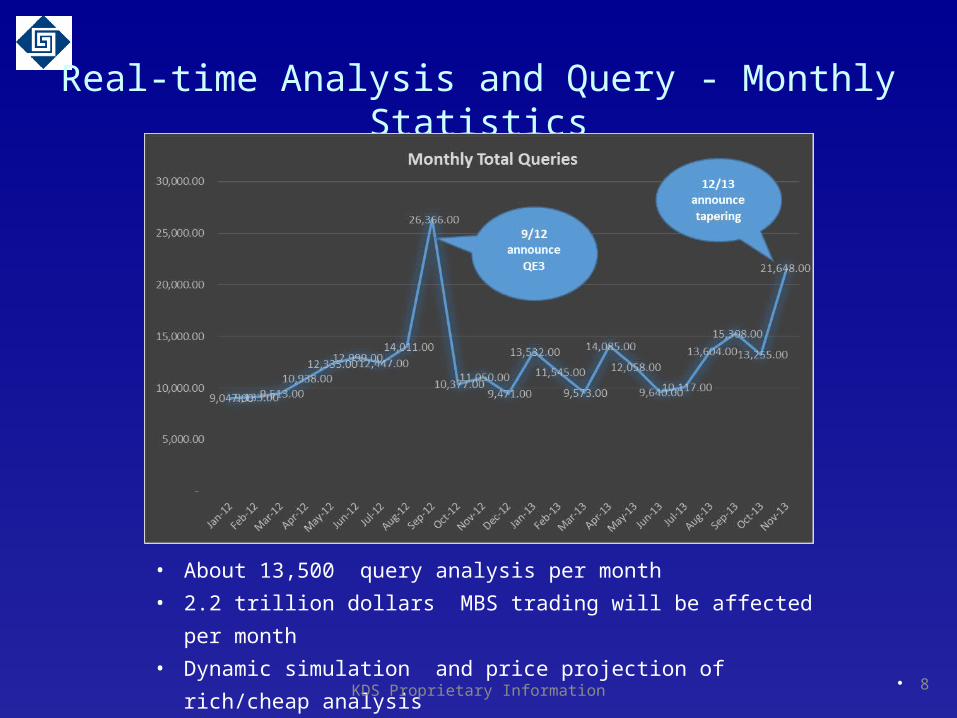
Real-time Analysis and Query - Monthly Statistics

• About 13,500 query analysis per month• 2.2 trillion dollars MBS trading will be affected per month• Dynamic simulation and price projection of rich/cheap analysis


• 9

Real-time Analysis•High efficiency, real-time•Provide market real-time snapshot to capture market movements.

• Flash Report

•Customize on-demand•Provide customized services for our clients• IOS Report

• Comprehensive, clear•Provide various statistics of market indicators to catch market dynamics.

• Servicer -Specpool

• KDS can provide timely and accurate market information, which serves as the crucial reference for tens of trillion dollars trading within seconds by Wells Fargo and other world's top financial institutions, and make huge profits.


Monte Carlo Workflow

IAS 39

PricingStructured Cashflow

Waterfalls (SCW)

Equity Pricing

+Prepayment

& Default Models

+

Interest Rate and HPA

Models: MC simulations or Rep Paths

for stress testing

Prepay

Delinquency

Roll Rates

Default

• Collateral

• (Residenti

Macro Economic Factors &

Assumptions:

Rates and HPA

FASB157

Hedging

Securitization

Loss Severity

Models Output Calculators Applications

Risk Mgmt

Input

Collateral

(Residential Mortgage

Loans)

MSR

10

Equity

+

Equity Derivatives

Equity Valuation

Equity On-Demand

Monte Carlo Simulations Model

Very fast convergence achieved with the combinations of:

High-dimensionality proprietary quasi-random number sequence (3x360 dimensions)

Proprietary controlled variate technique

Proprietary moment matching technique

11

MCS OAS Pricing Methodology Generate Monte Carlo Simulations (MCS) interest rate and HPA

up to 3000 paths at end-of-market, store in binary format to be used by OAS pricing programs.

Calibrate OAS spread matrix to Agency TBAs using KDS pool-level agency prepay models

Calibrate OAS spread matrix to most recent market surveys of benchmark ABS tranches (BC, ALT-A, JUMBO and Options ARM deals) using KDS loan-level prepay and loss models

Calibrate OAS spread matrix to most recent whole-loan transactions (market-driven, excluding distressed liquidations).

Run client MBS/ABS portfolios using calibrated OAS matrices on KDS’ proprietary 1024 CPU farm

12

• 13

Rich & Cheap Analysis – Monte Carlo Simulation

• GNR2013-122, CI

• GNR2013-122, PA


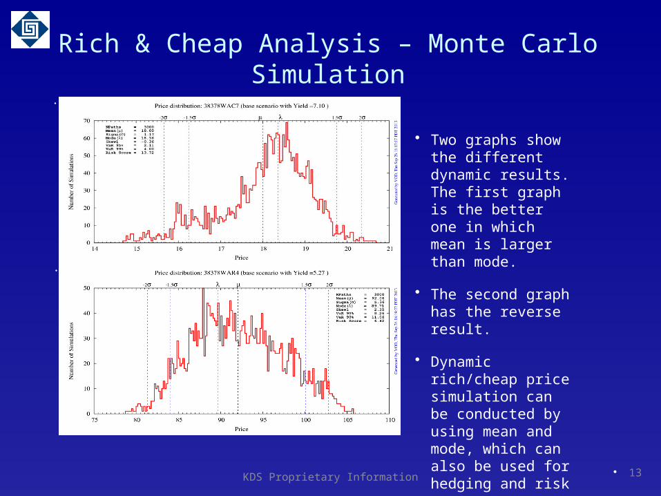
• Two graphs show the different dynamic results. The first graph is the better one in which mean is larger than mode.

• The second graph has the reverse result.

• Dynamic rich/cheap price simulation can be conducted by using mean and mode, which can also be used for hedging and risk management.

• 14

Rich & Cheap Analysis - Risk Measures

• GNR2013-122, PA

• GNR2013-122, CI


• 15

Rich & Chip Analysis - Cash Flow Holding

• Hedging and risk management strategy is based on the analysis of the projected cash flow.


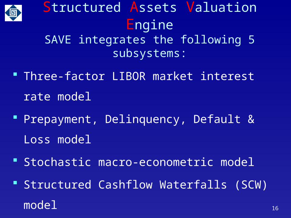
Structured Assets Valuation EngineSAVE integrates the following 5 subsystems:

Three-factor LIBOR market interest rate model

Prepayment, Delinquency, Default & Loss model

Stochastic macro-econometric model

Structured Cashflow Waterfalls (SCW) model

Monte Carlo Simulations (MCS) OAS model

16

Structured Assets Valuation Engine

Pre-Issuance Issuance Post-Issuance

ExtractionTranslation

Loading

Pool Optimization

PODDOD

Scripting Waterfall

Rosetta Stone

Bond Sizing

VODMCS_OAS

Econ Scenarios

Surveillance

Tax

AssetDatabase

17

Pip

elin

e M

anag

emen

tS

lice

& D

ice

RA

Lo

an L

oss

/Cre

dit

Mo

del

He

dg

ing

RA

Bo

nd

Siz

ing

Pri

cin

g/V

alu

ati

on

Collateral Data ETL Data Extraction, Transformation, and Loading

Remittance PDF report -> flash reports

80 ABX deals, 80 PrimeX deals, 125 CBMX deals

Custom defined deals remittance flash reports delivered real-time

Agency prepayment flash reports delivered real-time

Data Center Hosting on behalf of Clients:– Loan level data from LP, Intex, Lewtan– Loan level data from private firms

18

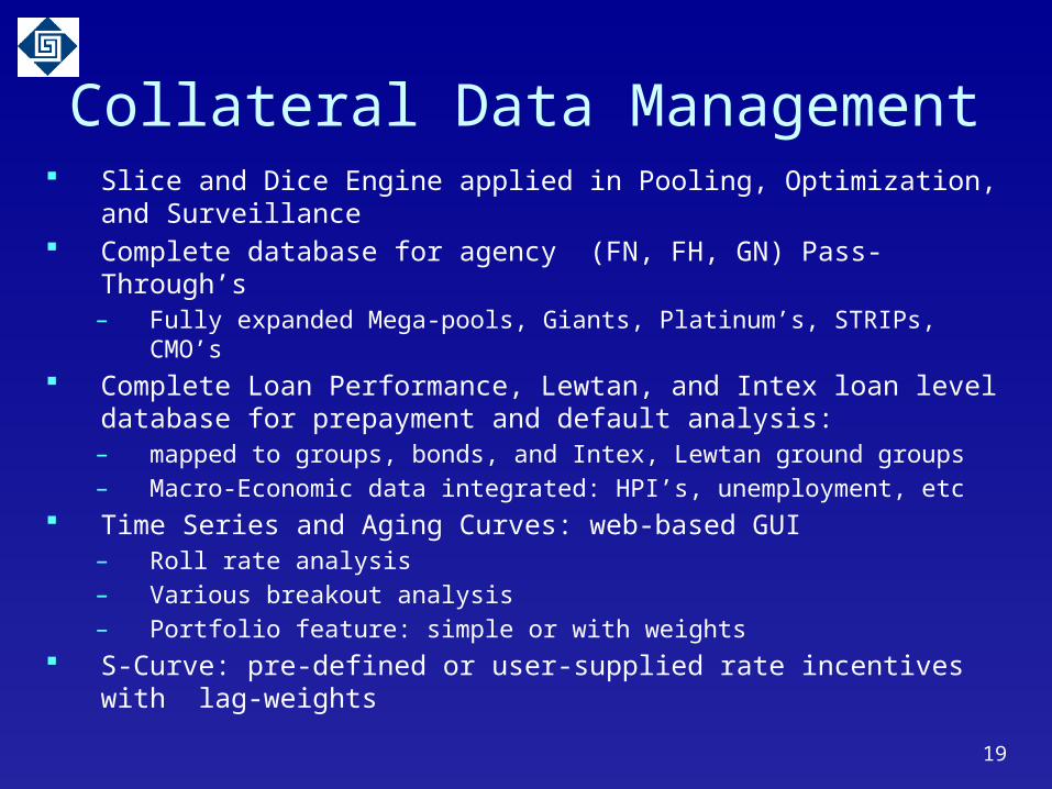
Collateral Data Management Slice and Dice Engine applied in Pooling, Optimization, and

Surveillance Complete database for agency (FN, FH, GN) Pass-Through’s

– Fully expanded Mega-pools, Giants, Platinum’s, STRIPs, CMO’s Complete Loan Performance, Lewtan, and Intex loan level database

for prepayment and default analysis:– mapped to groups, bonds, and Intex, Lewtan ground groups – Macro-Economic data integrated: HPI’s, unemployment, etc

Time Series and Aging Curves: web-based GUI – Roll rate analysis– Various breakout analysis– Portfolio feature: simple or with weights

S-Curve: pre-defined or user-supplied rate incentives with lag-weights

19

SCW Deal Structuring Collateral CF Engine

– Period based (amortization, scheduled payment/coupon, calendar, fee, OPT/ARM, Strips, Interest Reserve, Tax, etc..)

Scripting Engine– Python based waterfall programming with Customizable and Modulated

Script Command Call– Y/H/SEQ/ProRata/OC/Shifting-Interest– Credit Enhancement

Bond/Pool Insurance Policies Surety Bond Guarantee Derivatives (SWAP, Cap/Floor) Reserve Account

– Triggers Modules – DLQ, Loss– NAS/PAC/TAC– RE-REMIC– Pricing/Update/Payment Modes 20

SCW Deal Structuring Application

– Valuation On-Demand MCS_OAS Econ Scenarios

– Payment and performance surveillance & verification

– Risk Management Market Risk Hedging MSR

– REMIC (Projected) Tax

21

22

SCW Structuring Scripting ModuleSetDealParameters(('strike_rate', 5.05),

('index_name', 'LIBOR_1MO'),

('cuc_level_pct', 10),

('sen_enhance_threshold_pct', 40.20),

('stepdown_month', 37),

('oc_floor_pct', 0.50),

('oc_target_pct', 4.25),

('dlq_trigger_threashold_pct', 39.80),

('loss_trigger_threashold_pct', 1.35)

SetTrancheParameters(('A1A','A1B','A2','A3','A4','A5')

('target_paydown_pct',59.80)

)

SetTrancheParameters('A1A',

('cuc_multiplier', 2),

('coupon_spread', 0.17)

)

SetTrancheParameters('M1',

('cuc_multiplier', 1.5),

('coupon_spread', 0.30),

('target_paydown_pct',66.20)

# compute and swap flag and swap in/out amount

SetSwap()

# set bond coupon based CUC multipliers and coupon spread

SetCoupon(['A1A','A1B','A2','A3','A4','A5','M1','M2','M3','M4','M5','M6','M7','M8','M9'])

# compute stepdown flag from senior enhancement

SetStepDown(['A1A','A1B','A2','A3','A4','A5'])

# compute NEC

SetNetMonthlyExcessCF()

# compute DLQ trigger

SetDlqTrigger()

# compute loss trigger

SetLossTrigger()

# compute sequential trigger

SetSeqTrigger()

# compute principal distributions

SetPrincipalDistributions()

•BK

•PA

•BZ

•IA

•PA •IA

•PC •IC

•PD •ID

•PB •IB•PAC I

•PAC II• P

AC

I P

rin

cip

al

• PA

C II

Pri

nci

pal

•BK

•PA

•PB

•PC

•PD

• Re

ma

inin

g P

rin

cip

al

•Accretion•Principal

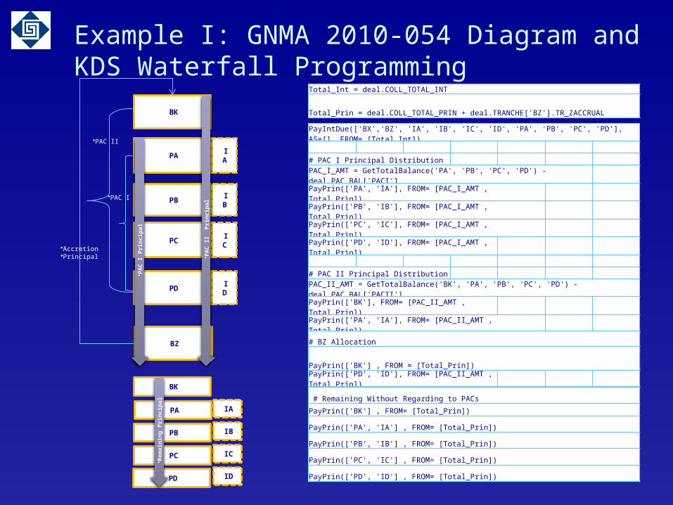
Total_Int = deal.COLL_TOTAL_INT

Total_Prin = deal.COLL_TOTAL_PRIN + deal.TRANCHE['BZ'].TR_ZACCRUAL

PayIntDue(['BX','BZ', 'IA', 'IB', 'IC', 'ID', 'PA', 'PB', 'PC', 'PD'], AS=[], FROM= [Total_Int])

# PAC I Principal Distribution

PAC_I_AMT = GetTotalBalance('PA', 'PB', 'PC', 'PD') - deal.PAC_BAL['PACI']

PayPrin(['PA', 'IA'], FROM= [PAC_I_AMT , Total_Prin])

PayPrin(['PB', 'IB'], FROM= [PAC_I_AMT , Total_Prin])

PayPrin(['PC', 'IC'], FROM= [PAC_I_AMT , Total_Prin])

PayPrin(['PD', 'ID'], FROM= [PAC_I_AMT , Total_Prin])

# PAC II Principal Distribution

PAC_II_AMT = GetTotalBalance('BK', 'PA', 'PB', 'PC', 'PD') - deal.PAC_BAL['PACII']

PayPrin(['BK'], FROM= [PAC_II_AMT , Total_Prin])

PayPrin(['PA', 'IA'], FROM= [PAC_II_AMT , Total_Prin])

PayPrin(['PB', 'IB'], FROM= [PAC_II_AMT , Total_Prin])

PayPrin(['PC', 'IC'], FROM= [PAC_II_AMT , Total_Prin])

PayPrin(['PD', 'ID'], FROM= [PAC_II_AMT , Total_Prin])

# BZ Allocation

PayPrin(['BK'] , FROM = [Total_Prin])

# Remaining Without Regarding to PACs

PayPrin(['BK'] , FROM= [Total_Prin])

PayPrin(['PA', 'IA'] , FROM= [Total_Prin])

PayPrin(['PB', 'IB'] , FROM= [Total_Prin])

PayPrin(['PC', 'IC'] , FROM= [Total_Prin])

PayPrin(['PD', 'ID'] , FROM= [Total_Prin])

•IA

•IB

•IC

•ID

Example I: GNMA 2010-054 Diagram and KDS Waterfall Programming

24

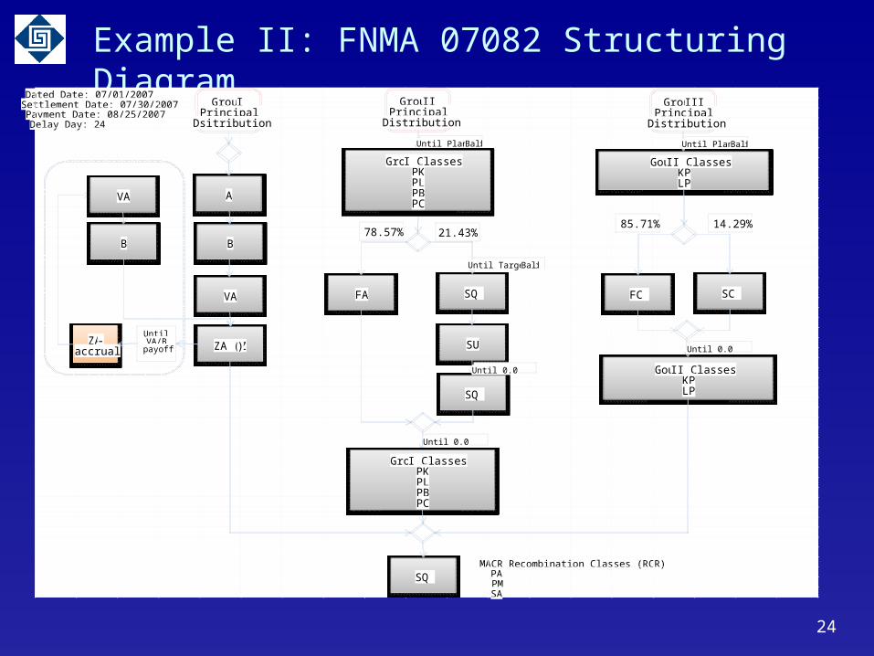
Example II: FNMA 07082 Structuring DiagramDated Date: 07/01/2007Settlement Date: 07/30/2007Payment Date: 08/25/2007Delay Day: 24

MACR Recombination Classes (RCR)PAPMSA

ZA (Z)

A

B

VA FA SQ

SU

SQ

FC SC

GourpII ClassesKPLP

GroupI Principal

Dsitribution

GroupII Principal

Distribution

GroupIII Principal

Distribution

ZA-accrual

Until VA/B

payoff

78.57% 21.43%

Until PlannedBal

Until Targeted Bal

GroupI ClassesPKPLPBPC

GroupI ClassesPKPLPBPC

GourpII ClassesKPLP

Until PlannedBal

85.71% 14.29%

Until 0.0

Until 0.0

Until 0.0

SQ

VA

B

25

Example III:JP MORGAN MORTGAGE TRUST 2007-CH3

Closing Date 5/15/2007 Collateral Type

– Subprime Home Equity Capital Structure:

– Overcollateralization– SEN/MEZZ/JUN Y Structure– Net SWAP cover OC Deficiency, Interest Shortfall, Realized

Loss, NetWAC Carryover– Cross-Collateralization

Triggers in – Enhancement Delinquency– Cumulative Loss– Sequential Trigger– OC and Subs Test

26

Example IV:NEW CENTURY HEL TRUST 2006-2

Closing Date 06/29/2006 Collateral

– Subprime Home Equity Capital Structure:

– Overcollateralization– SEN/JUN Sequential– Net SWAP cover OC Deficiency, Interest Shortfall, Realized Loss,

NetWAC Carryover– Cross-Collateralization (on Group I & I Notes Sen)

Triggers in – Enhancement Delinquency– Cumulative Loss– Sequential Trigger– OC and Subs Test

RMBS Valuation Models Prepay, Default, Severity, Delinquency

– Modeling Approach Delinquency Transitions Prepay/Default Competing Risks

– Agency and Non-Agency Collateral: Prime Jumbo Alt-A Option ARM Subprime HELOC Fannie/Freddie FHA/VA

27

TBA Analytics

– De Facto Standard Pool pricing– Worst to Delivery Slice-and-Dice and Priding– Absolute value: Yield to Maturity, OAS, Total Return– Relative value: return vs. other securities (corporate bonds,

swaps, agency debt, etc.), vs. sector benchmark (TBA, current coupon, index), vs. intra-sector alternatives (vs. Gold, vs. GN, vs. 15-year, etc.)

– Historical rich/cheap analysis: time series mean reversion

28

CMBS Valuation Models Prepay, Default, Timing of Default, Severity, Extension

– Key Inputs: Property Type, LTV, DSCR, NOI, Underwriting,

MSA, Cap Rate, Refi Threshold, Call Protection, Tenant Attributes

– Subsystems APOLLO: NOI Generator, Scenario/Monte Carlo Simulation HELIOS: Loan Level Prepay/Default Generator

Market Calibration– CMBX, TRX– Conversion from TRX to OAS

29

30

• For each CMBS deal in the portfolio, the underlying loans and properties are identified and passed into the loan-level analysis and pricing engine.

• Property Analyzer breaks down

collateral pools into property types by

MSA

• OFFICE

• RETAIL

• MULTI-FAMILY• HOTEL

• INDUSTRIAL

• HEALTH-CARE

• SELF-STORAGE

• NOI PROJECTION• NOI PROJECTION• NOI PROJECTION• NOI PROJECTION• NOI PROJECTION• NOI PROJECTION

• NOI PROJECTION

• Baseline NOI time-

series projected

per property

type

• Ex) MSA: New York

• Property and tenant

database tracks and monitors high-risk loans and tenants.

• DYNAMIC CALIBRATION : Defines initial NOI surface for all properties in portfolio, and

utilizes the Baseline NOI feed to define Specific (Absolute) NOI Projections for all properties in

portfolio.

• Loan-level NOI projections

translated into loan-level

Implied DSCR Projections

• CREDIT MODEL: Projects loan-level defaults, timing of defaults and

liquidations, and loss-given-defaults, based on DSCR curves and baseline

severities provided. Extensions, work-outs, and loan-modifications are also

projected at this step. Manual overrides on defined parameters are possible.

• Data source containing latest

and historical performance data

for CMBS/CRE properties

• OFFICE

• RETAIL

• MULTI-FAMILY• HOTEL

• INDUSTRIAL

• HEALTH-CARE

• SELF-STORAGE

• BASE SEVERITY• BASE SEVERITY• BASE SEVERITY• BASE SEVERITY• BASE SEVERITY• BASE SEVERITY

• BASE SEVERITY

• Baseline SEVERITY (given default) values

projected per property type

• REAL ESTATE DATA

• PREPAYMENT MODEL: Prepayment projection curves generated for all loans, based on property details (e.g. type,

geography, call protection, etc.)

• PRICING MODEL: Utilizes information and projections from

component models to setup pricing scenarios for each CMBS

deal in the portfolio, and interacts with KDS cash flow engine to

produce price/cash flow projections for the corresponding

CMBS tranches.

• DISCOUNT MARGIN: Pricing spreads are

determined based on CMBS deal performance,

default behavior, and market data.

• LARGE

CMBS PORTFO

LIO•

DYN

AMIC

CM

BS M

OD

EL

• MARKET DATA • KDS Cash-flow

Model

• CMBS

PRICING

REPORT

• Main Input/Output File• External data source• KDS low intensity computing module• KDS moderate intensity computing module• KDS high intensity computing module• External pricing engine• Baseline projections/scalars, generated in-house or obtained via subscription (e.g. PPR)

• LEGEND


Index Derivative Analytics

Complete coverage in PRIMEX, ABX, CMBX, MBX/IOS/PO

Calculate Market Implied Spread(OAS) based on Economic Scenarios and 3000 paths Monte Carlo Simulation

Monte Carlo Simulation based risk measures in – Mode– Skewness (Pearson's first)– Mean – Sigma – Var – 1-dVar– Risk Score

Daily and Weekly Reports based on Market Close Price

31

Agency Index Daily Report

32

TBA Daily Report

33

Prepay/Default/Severity Overview

Projects monthly prepayment, delinquency, default and loss severity rates of new (at purchase) or seasoned (portfolio) loans.

Takes into account of loan, borrower and collateral risk characteristics as well as macro economic variables on rates and home prices.

Based on a hybrid delinquency transition rate and competing risks survivorship model where the prepay & default risk parameters are estimated from historical loan-level data.

34

Based on a proprietary highly non-linear non-parametric methodology with parameters estimated from non-agency loan-level data.

Prepay and default are jointly estimated in a competing risk framework.


35

Model Inputs – Collateral type (e.g., alt-a, non-conforming balance, no prepay

penalty).– Age, Note rate, Mortgage rates, Yield curve slope.– Home price (zip/CBSA-level if used at loan-level, otherwise state-

or national-level)– Unemployment rate– Loan size, Documentation, Occupancy, Purpose, State, FICO, LTV,

Channel.– Delinquency history and status (past due, bankruptcy, REO)– Negative amortization limit (recast) for option ARM– Modification type, size, and timing– Servicer


36

Model Outputs

– Prepayment and default probabilities at each time step

– Delinquency rates

– Loss severity


37

All forward curves are generated using proprietary non-parametric calibration technique that is guaranteed with maximum smoothness

The forward curves are consider “trading quality” and “battle tested” have been by various trading desks for trades in excess of $1T worth of derivatives

These should not be compared with forward curves from

Bloomberg where they are only for informational purposes, or with many leading Asset/Liability software venders where the forward curves are usually used for monthly portfolio valuation (i.e., accounting purposes) rather than for trading purposes

Derivative Hedging On-Demand

38

All flavors of interest rate swaps (including swaps with embedded options, both European and Bermudan)

Swaptions (European, Bermudan and/or custom) LIBOR, CMS/CMT caps/floors CMM (constant maturity mortgage) swaps, FRAs (forward

rate agreements), and swaptions (this includes our mortgage current model)

Mortgage options Treasury note/bond futures and options Other customized derivatives


39

40


Equity On-Demand

41

• Hedge-funds and investment banks that develop these type of tools to capture mispricings in equity derivatives markets keep them proprietary and do not share with them anyone.

• The KDS option model and trading platform, also known as EOD, tackles all of these challenges and makes the proper tools available for traders so that they can profit from mispricings everyday!

• The EOD allows traders to wake up in the morning with trading strategies that are indifferent to whether the market is bullish or bearish. Instead, they can focus on profiting using high probabilities in both up and down markets. This eliminates trading based on human emotion, which is the cause for most financial mistakes!

• The Bullish vs. Bearish paradigm was created by the Technical Model mindset. Using volatility based analysis and high-probability trading means that the so-called “Bullish” or “Bearish” trade is no longer meaningful, and profitability does not depend on the direction of the market!

• In this presentation, we will cover the different parts of the EOD system, describe how to use the system, and most importantly show how to execute trading strategies and make money consistently using the EOD.

EOD Option Pricing EOD platform utilizes advanced option pricing models.

Based on trader’s “Risk Appetite,” he or she can use EOD to create trading strategies such as:– High Probability Mean Reversion strategies– Time decay (Theta) strategies– Spread based strategies (vertical/calendar spreads)– Underlying ETF buy/sell strategies

“Risk Appetite” is based on confidence levels, or probability ranges, that are used for mean-reversion trades and also allow traders to tweak their risk tolerance using precise metrics.

For example, a confidence level gives the trader ability to know the exact probability that a buyer of an option will exercise, at any given time. This is very important for HPMR trades!

EOD successfully eliminates subjectivity from options trading by specifying strike price targets and buy/sell thresholds.

42

Pricing Methodologies

Our underlying option models use advanced techniques from quantum physics and nonlinear mathematics, applied to financial analysis and trading.

The models are applied to finance using fundamental laws of physics and mathematics, and utilize coordinate transformations in Space, Time, Force, Momentum, and Energy.

Since option prices have diffusion properties, we can use systems of partial differential equations to model price behavior.

We model the randomness observed in prices and volatilities by using stochastic frameworks such as Variance Gamma and Long-Range Stochastic Volatility (discussed later).

Since solutions to these stochastic and highly nonlinear system of PDE’s are unsolvable via analytical methods, we must utilize massive parallel-processing computational power to run extremely large numbers of scenarios at infinitesimal (intra-day) time steps.

43

Pricing Methodologies REAL-TIME probability distributions of option prices, as well as REAL-TIME

option chains pricing solutions, are calculated through evaluating the large number of intra-day scenarios.

Unlike EOD, most option pricing models in the market-place use Black-Scholes-Merton (BSM) framework as the underlying theory.

There are many problems with using this BSM framework to do real-time options trading, most importantly:– Probability distributions do not have FAT-TAILS as observed in the markets.– Prices utilize a single volatility, which is clearly not true in reality.– BSM framework does not have ability to imply a Volatility Skew or Volatility Smile.– BSM framework was created for European-style options which can only be exercised

at maturity. In reality, most ETFs that trade on exchanges are American-style, which can be exercised any time.

– There is no ability to capture and quantify JUMPS (both up and down) in prices of options and underlying Equity Index/ETF.

– BSM Equations were designed by professors (not traders) to allow “analytical solutions” for their convenience. In practice, we don’t care about elegant “analytical solutions” if the prices are WRONG!

44

45

American Short-Range Jump Diffusion Model: 100K Pricing Paths for IWM (iShares Russell 2000 Index)

Volatility Surface Smile: TZA vs. TNA

• The volatility surface of the inverse 3x leverage TZA compared against the positive 3x leverage TNA indicates an inverse relationship.

• However, the relationship is not precisely inverse due to the fact that both TZA and TNA are separate tradable securities, with unique option chain dynamics.

• Therefore, we are able to capture not only the intrinsic inverse relationship, but also the individual supply/demand dynamics for each ETF.

Volatility of Volatility (VXX Surface)

48

American Short-Range Jump Diffusion Model

In addition to Stochastic Volatility, the VGSV based framework enables us to price options using American exercisability.

The American exercise feature utilizes a Least-Squares Monte Carlo (LSM) methodology which iteratively quantifies the probability of exercise PER timestep.

VGSV framework also allows us to model the Jump up and Jump down impact under a Short-Range (i.e. intra-day) time period.

Jump processes are modeled via the sampling of gamma and exponential distribution variates over a large number of paths and trajectories.

For these reasons, we also refer to our option pricing model as the American Short-Range Jump diffusion (ASD) model.

For the long-range (20+ days) option chains, we utilize the America Long-Range Jump diffusion (ALD) model which allows us to capture the longer term convergence properties of option pricing.

Fat-Tail Distributions

EOD uses proprietary methods based around Short-Range Variance Gamma stochastic volatility (VGSV) and Long-Range stochastic volatility models.

Within our framework, we are able to produce probability distributions that accurately capture the FAT-TAILS (left and right) implied by the market.

Since most of the mispricings (i.e. Money-Making Opportunities) exist near the TAILS of the distribution (OTM options), precisely capturing fat-tails is VERY IMPORTANT!

The REAL-TIME display of the probability distributions (“Histograms”) allows traders to not only see the fat-tails, but also track how the area under the fat-tails is shifting in REAL-TIME.

Having this fat-tail probability distribution framework allows us to effectively DISCOVER the market inefficiencies throughout the trading day.

49

Interest Rate Model

Three-Factor BGM/Libor Market Model (LMM)

Forward curve calibrated to a daily mixture of Libor, Euro$ Futures, Euro$ futures options, and intermediate to long term swap rates

Volatility calibrated to daily end-of-market swaption volatility surface

The “battle tested” forward curves for trading & valuations are guaranteed with the maximum smoothness.

50

51

Libor Market Model

Also known as the BGM (Brace-Gatare-Musiela) model.

It is the “modern” implementation of the well-known Heath-Jarrow-Morton Model

Considered the “second-generation” of interest rate models. The “first-generation” being the Hull-White family of short-rate models

52

Key Features of Libor Market Model

Model construction is automatically arbitrage free.

No need for yield curve calibration. Avoided the problem of convergence when calibrating most type of short rate models.

Intuitive volatility and correlation calibration.

Can accommodate arbitrary number of factors in a straight forward way.

53

Libor Market Model vs. Traditional Short Rate Models

No need to iteratively search for a set of calibration parameters in order to match the yield curve.

E.g., Hull-White model is calibrated to the first-derivative of the forward curve, which can be oscillatory sometimes. LMM does not suffer from this problem.

For most short-rate models, rates would have to be sampled from some simple lattice (either binomial or trinomial). I.e., rates can only go up or down, but not from a normal distribution.

54


Can sample from short rate model equations using normal distribution, but since the model parameters are calibrated on the lattice, “equation sampling” will not be arbitrage free, i.e, incorrect in most cases.

No need for mean-reversion parameter in LMM, which has no true economic meaning (see “Interest Rate Option Models”, R. Rebonato). Therefore no need to calibrate the model to this artificial parameter.

Volatility calibration is more intuitive in LMM vs. short rate models (see papers by the author of LMM, and John Hull).

55


Multifactor version of the short rate models are limited to two-factor models. Calibrating these models to market instruments are extremely difficult (see “Interest Rate Option Models”, R. Rebonato).

Because of this difficulty, virtually no software vendors offers this functionality except a select few such as Numerix (expensive…) and some Wall Street trading desks. QRM has a “place holder” for a two-factor model, but I was told it’s essentially useless and no client uses it.

56


LMM/HJM models have been adopted by more Wall Street MBS trading desks recently, as they “upgrade” from the older short rate models.

Quote from J. Hull’s book (the author of most short-rate models):

“because they are heavily path dependent, mortgage-backed securities usually have to be valued using Monte Carlo simulation.

These are therefore ideal candidates for applications of the HJM model

and Libor market models”.

57

Competitor I Interest Rate Models Single-Factor Black-Karasinski (BK) Single-Factor Hull-White (HW) Better suited for lattice-based pricing applications, such as

Bermudan Swaptions, CMS cap/floors, etc. ; issues with arbitrage-free in a simulation setting because parameters are calibrated on the lattice but Monte Carlo rates are generated from the stochastic equation (see J Hull book on this issue).

Volatility and mean-reversion parameters in Competitor I’s versions of BK & HW are “user inputs”, instead of optimized to fit a series of market option prices (see extensive discussion on this issue in J. Hull’s book); this could problematic because the mean reversion parameter does not have intuitive true economic meaning.

Interest rate models are not truly arbitrage-free by design (this is separate from the sampling error issue of Monte Carlo), and the mean-reversion and volatility parameters are not calibrated to market vols.

58

Competitor II Interest Rate Models Prepayment model is not up to standard.

The turnover and refi components are not handled well. The refi component is part of prepayment model deals with

interest rate sensitivity. Burnout/season component part of the model is also not

handled well.

Duration result is off from market expectation. This most likely has to do with its prepayment model and it's

interest rate model. OAS/interest rate model uses its own version of the lognormal

model. It is quite different than either the HJM class of the HULL White

class of models. Besides prepayment models, duration calculation can also be

sensitive to one's implementation of the OAS/interest rate model.

59

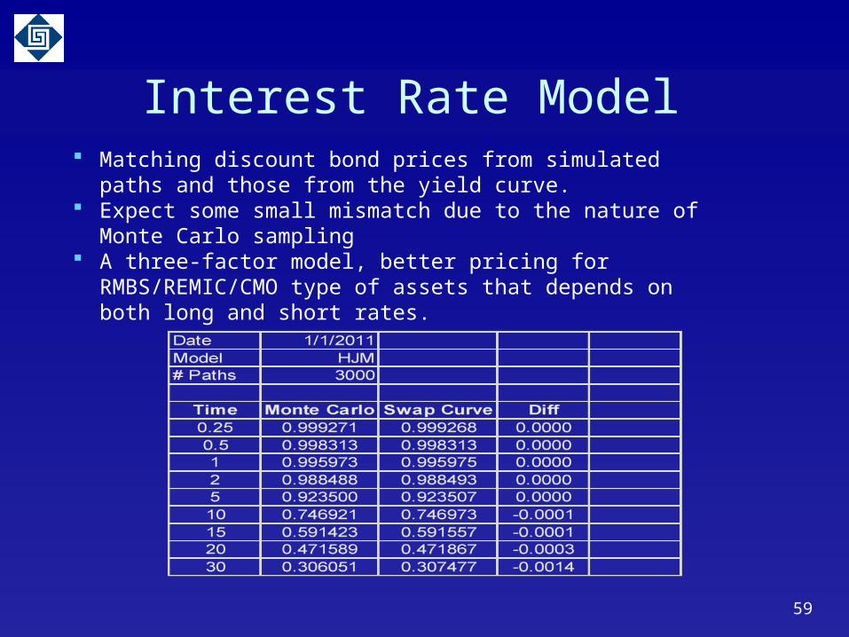
Matching discount bond prices from simulated paths and those from the yield curve.

Expect some small mismatch due to the nature of Monte Carlo sampling

A three-factor model, better pricing for RMBS/REMIC/CMO type of assets that depends on both long and short rates.

Interest Rate Model

Interest Rate Model

60

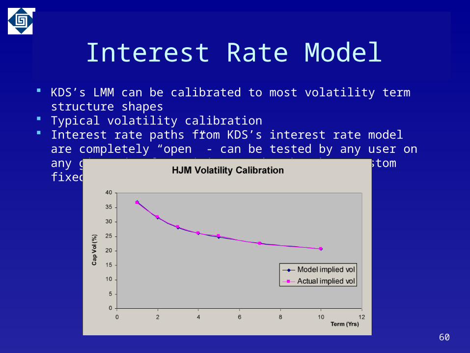
KDS’s LMM can be calibrated to most volatility term structure shapes Typical volatility calibration Interest rate paths from KDS’s interest rate model are completely

“open” - can be tested by any user on any given day for pricing any benchmark or custom fixed income assets.

Interest Rate Model Summary

61

Interest rate modeling is at the center of interest rate risk management.

Sophisticated interest rate risk management demands state-of-the art interest rate models.

Libor Market/HJM models are current state-of-the art and ideally suited for pricing and risk managing mortgage securities.

Home Price Model

HPA Projection

0

50

100

150

200

250

1989 1994 1999 2004 2009 2014 2019

HP

A (

%)

Mean-reverting

Targets long-term HPA using a historical “mean”.

Mean-reversion parameters tunable for faster or slower reversion.

62

63

Personal Income & HPI Forecast

64

HPA Scenarios

65

Unemployment Scenarios

• 66

Technology


UBX Architecture


• Network Attached

• Internet, Intranet, Extranet, IP Packet Network, • Optical Network

• N

• SysGovernor

• Client Browser

• 1

• N

• 1• Web Engine

• FTP Server

• Internet, Intranet, Extranet, IP Packet Network, • Optical Network

• N

• Super• SysGovernor

• Client Browser/Apps

• 1

• N

• 1 • Web Engine

• OLTP Database

• FTP Server

• Fiberoptic Switching Complex

• Fiberoptic Switching Complex

• Existing

• ComputeNode• 1

• Index• 1

• Data Set• 1

•

• 8 CPU• 64GB

RAM• SSD

Cache• HAV CPU Node • HAV CPU Node

• CPU + GPU• 64GB RAM• SSD Cache• CPU + GPU

• 64GB RAM• SSD Cache

• GPU Enhanced Compute Nodes

• GPU Enhanced Compute Nodes

• Existing


• Index• 1

• Data Set• 1

•

• 8 CPU• 64GB

RAM• SSD

Cache

• Existing


• Index• 1

• Data Set• 1

•

• 8 CPU• 64GB

RAM• SSD

Cache

• HAV: High-Availability Virtualization based on Xen Cloud Platform (XCP) • HAV: High-Availability Virtualization based on Xen Cloud Platform (XCP)

• HAV CPU Node • HAV CPU Node • HAV CPU Node • HAV CPU Node

• Gigbit Ethernet Switch

• Gigbit Ethernet Switch

• HAS: N+3 redundancy, SSD buffer,High Availability Storage

• HAS: N+3 redundancy, SSD buffer,High Availability Storage

HAS: High AvailabilityStorage Complex

• 68

UBX Advantage

Index: Index all the data by UBX sorter.

– Index take only 40% storage

– Randomly search abilities

– Easy maintenance

Parallel Model: several parallel optimization methods can be carried on in UBX:

– Local Optimization: NLIN, SLSQP, LSBFGS, COBYLA, BOBYQA, etc

– Global Optimization: DIRECT, CRS, StoGO, ISRES, etc

– Used to calibrate the QED Pricing Model

Flexibility: new business rules and definitions can be implemented within minutes using high performance scripting languages

Efficiently take advantage of open source module


UBX Advantage

High-speed data acquisition: Use core system function to reduce unnecessary cost.

High Volume Data: Overlapping I/O tasks with computation tasks.

Parallelism: Large datasets are partitioned into smaller portions and processed in parallel on multiple computational nodes.

Expansibility: As a result of the inherent parallelism of our model, as more nodes are added, larger datasets can be processed at reduced time.

Streaming: Multivariate solution is done in a scan.


UBX Advantage

SPMD: Single Process Multiple Data, data mining, VOD

MPMD: Multiple Process Multiple Data, model calibration, MCS

Virtual fields: fields can be mathematical formula to save storage and extend the usage

Table Join: table can be joined to re-use existing fields Table can be combined horizontally and vertically to extend the

usage


UBX Advantage

Virtual Tables: tables can be combined to form virtual logical tables


• UBFile1

• UBFile2

• UBFileN

• UBFile1

• UBFile2

• UBFileN

• Vertical File: Horizontal File:

• Combined Table


UBX: The Sweet Spot

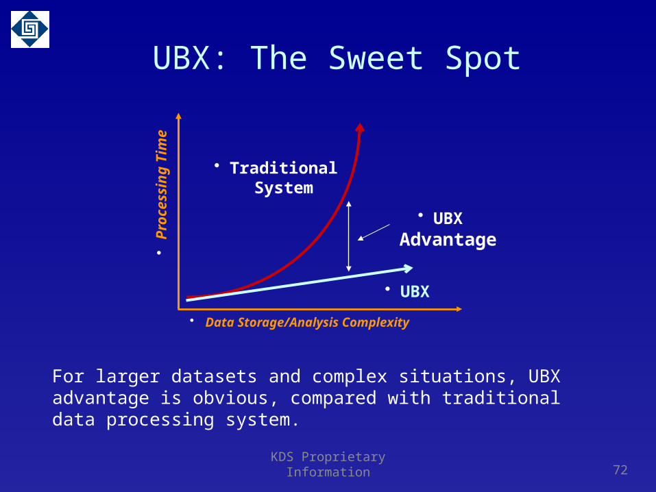
For larger datasets and complex situations, UBX advantage is obvious, compared with traditional data processing system.

• UBX Advantage

• Data Storage/Analysis Complexity

• UBX

•P

roce

ssin

g

Tim

e • Traditional System

Nonlinear Least Square Regression Benchmark Performance

No. of Record Date Size(MB)

Number Node Nonlinear Cycles

Time (s)

45,889 3.15 1 6 9 5

4,254,142 09/00 - 08/01 896.61 12 6 8 288

8,243,801 09/99 – 08/01 1,737.48 24 6 8 353

12,606,708 09/98 – 08/01 2,657.02 36 6 8 456

19,953,262 09/96 – 08/01 4,205.39 60 6 8 682

24,621,612 09/94 – 12/00 5,189.30 83 6 8 709


0

100

200

300

400

500

600

700

800

0 5,000,000 10,000,000 15,000,000 20,000,000 25,000,000

Number of records

Tim

e in

se

con

ds

• Traditional System

• UBX

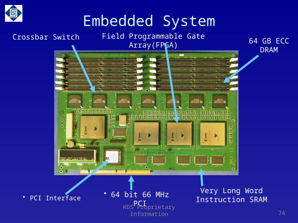
Embedded System

• 64 bit 66 MHz PCI Very Long WordInstruction SRAM

Crossbar Switch Field Programmable Gate Array(FPGA)64 GB ECC

DRAM

• PCI Interface


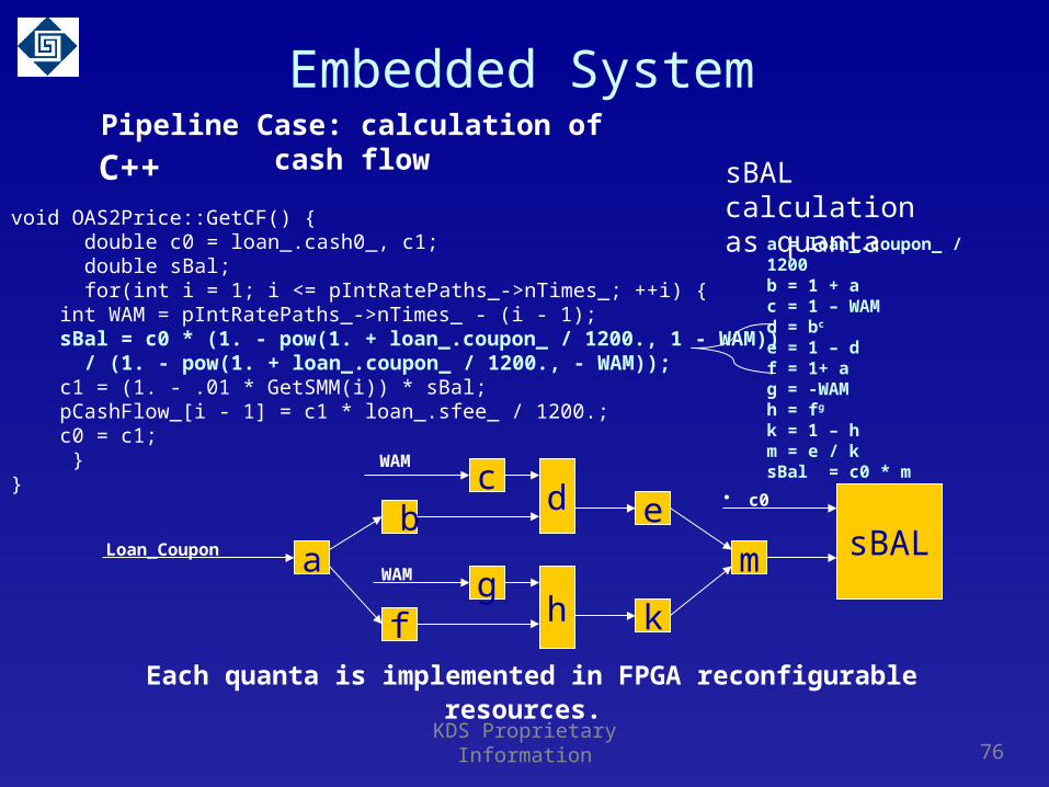
Embedded SystemPipeline Case: calculation of cash flow

void OAS2Price::GetCF() {

double c0 = loan_.cash0_, c1;

double sBal;

for(int i = 1; i <= pIntRatePaths_->nTimes_; ++i) {

int WAM = pIntRatePaths_->nTimes_ - (i - 1);

sBal = c0 * (1. - pow(1. + loan_.coupon_ / 1200., 1 - WAM))

/ (1. - pow(1. + loan_.coupon_ / 1200., - WAM));

c1 = (1. - .01 * GetSMM(i)) * sBal;

pCashFlow_[i - 1] = c1 * loan_.sfee_ / 1200.;

c0 = c1;

}

}

1,641 clock ticks for eachIteration of the for loop


The time quanta for the FPGA is equal to 10 clocks of a 1GHZ processor. For this example the embedded system is about 160 times faster then the C++ open environment. The rate of completed calculations is independent of the analysis complexity and the data size.

Pipeline Case: calculation of cash flow

void OAS2Price::GetCF() { double c0 = loan_.cash0_, c1; double sBal; for(int i = 1; i <= pIntRatePaths_->nTimes_; ++i) { int WAM = pIntRatePaths_->nTimes_ - (i - 1); sBal = c0 * (1. - pow(1. + loan_.coupon_ / 1200., 1 - WAM)) / (1. - pow(1. + loan_.coupon_ / 1200., - WAM)); c1 = (1. - .01 * GetSMM(i)) * sBal; pCashFlow_[i - 1] = c1 * loan_.sfee_ / 1200.; c0 = c1; }}

a = loan_.coupon_ / 1200b = 1 + ac = 1 – WAMd = bc

e = 1 – d f = 1+ ag = -WAMh = fg

k = 1 – hm = e / k sBal = c0 * m

C++ sBAL calculationas quanta

f

bc

gh

d

k

e

m sBALaLoan_Coupon

WAM

• c0

Each quanta is implemented in FPGA reconfigurable resources.

WAM


Embedded System

WAM

f

bc

g h

d

k

em sBALaLoan_Coupon

WAM

WAM

c0CLOCK TICK 1

f

bc

g h

d

k

em sBALaLoan_Coupon

WAM

WAM

c0CLOCK TICK 2

CLOCK TICK 3

f

bc

g h

d

k

em sBALaLoan_Coupon

WAM

c0

At each time tick the data moves to the next calculation.A data calculation is completed for each time tick.


Embedded SystemPipeline Case: calculation of cash flow

• 78

Competitive Expertise


Expertise on Marketable Securities

• Marketable securities• U.S. agency mortgage backed securities (Fannie, Freddie, Ginnie)• Non agency mortgage backed securities (private label)• Collateralized debt obligations (CDOs)• Securitization of assets

• Valuation on demand platform• Massive database on U.S. securities• Real time feed of market information• Advanced interest rate model and forward curve• Multiple variable credit and prepayment models


Expertise on Consumer Lending

• Lending products• Residential mortgage loans• Consumer and small business credit card loans• Peer-to-peer installation loans

• Extensive in-depth management experience• Marketing solicitation• Credit underwriting• Portfolio management• Collection strategies• Basel II implementation• Credit risk scoring• Credit bureau management


Expertise on Derivative Valuation

• Derivative instruments• Swap• European Swaption• American Swaption• Floating rate bond• Fixed rate bond• Cap floor

• Valuation on demand platform• Advanced interest rate model• Market calibrated forward curve• New quantum field pricing model• Counterparty Valuation Adjustment (CVA)


knowledge decision securities, llc. kds confidential & proprietary information. do not...

Documents

curve loan

data structures

loss slide

loss data hosting platform

tb loanasset pool data

knowledge decision securities

time series aging curve

patented ubx sorter