Preprint typeset in JHEP style - HYPER VERSION

Knots-quivers correspondence

Piotr Kucharski1, Markus Reineke2, Marko Stosic3,4, and Piotr Su lkowski1,5

1 Faculty of Physics, University of Warsaw, ul. Pasteura 5, 02-093 Warsaw, Poland2 Faculty of Mathematics, Ruhr-Universitat Bochum, Universitatsstrasse 150, 44780

Bochum, Germany3 CAMGSD, Departamento de Matematica, Instituto Superior Tecnico, Av. Rovisco Pais,

1049-001 Lisboa, Portugal4 Mathematical Institute SANU, Knez Mihailova 36, 11000 Beograd, Serbia5 Walter Burke Institute for Theoretical Physics, California Institute of Technology,

Pasadena, CA 91125, USA

Abstract: We introduce and explore the relation between knot invariants and quiver

representation theory, which follows from the identification of quiver quantum mechanics

in D-brane systems representing knots. We identify various structural properties of quivers

associated to knots, and identify such quivers explicitly in many examples, including some

infinite families of knots, all knots up to 6 crossings, and some knots with thick homology.

Moreover, based on these properties, we derive previously unknown expressions for colored

HOMFLY-PT polynomials and superpolynomials for various knots. For all knots, for which

we identify the corresponding quivers, the LMOV conjecture for all symmetric representations

(i.e. integrality of relevant BPS numbers) is automatically proved.

CALT-2017-040

arX

iv:1

707.

0401

7v1

[he

p-th

] 1

3 Ju

l 201

7

Contents

1. Introduction 2

2. Knot theory and physics 5

2.1 Knot invariants and the LMOV conjecture 5

2.2 Knot homologies 8

3. Quiver moduli and Donaldson-Thomas invariants 10

4. Knot invariants from quivers 12

4.1 Main conjectures 12

4.2 Superpolynomials and quadruply-graded homology of knots from quivers 15

4.3 Consequences: proof of the LMOV conjecture, new categorification, etc. 16

4.4 The strategy and q-identities 17

4.5 Reduced vs. unreduced invariants 19

5. Case studies 20

5.1 Unknot 20

5.2 Trefoil and cinquefoil knots 21

5.3 (2, 2p+ 1) torus knots 24

5.4 (2, 2p) torus links 27

5.5 (3, p) torus knots 29

5.6 Twist knots 41, 61, 81, . . . 32

5.7 Twist knots 31, 52, 72, 92, . . . 34

5.8 62 and 63 knots 37

– 1 –

1. Introduction

BPS states in supersymmetric field theories and string theory have remarkable properties,

which have been actively studied in last decades. In this paper we consider BPS states that

arise in D-brane systems, which encode properties of knots. The counting of these states leads

to invariants of knots, referred to as Labastida-Marino-Ooguri-Vafa (LMOV) invariants (or

Ooguri-Vafa invariants). On the other hand, dimensional reduction of such brane systems is

expected to lead to a description in terms of a supersymmetric quiver quantum mechanics. In

this paper we argue that this is indeed the case, and in consequence properties of BPS states

are encoded in the data of moduli spaces of quiver representations, which leads to intriguing

relations between knots and quivers. We presented a general idea of this correspondence

in [1]. Now, in this paper, we explain more details of the identification between knot invari-

ants and quiver moduli spaces, which enables us to identify explicitly relevant quivers for

many knots, including some infinite families of knots, all knots with up to 6 crossings, some

knots with thick HOMFLY-PT homology, etc. Understanding structural properties of gener-

ating series of knot polynomials also enables us to derive previously unknown expressions for

colored HOMFLY-PT polynomials and superpolynomials (and their quadruply-graded gener-

alizations) for several knots. More importantly, our correspondence relates generating series

of colored HOMFLY-PT polynomials to motivic Donaldson-Thomas (DT) invariants, which

then leads to the proof of the famous integrality of LMOV invariants, conjectured in [2–4]. We

also discuss many other consequences of the relation between BPS states, knots and quivers.

Both types of invariants mentioned above, i.e. LMOV invariants of knots and motivic

Donaldson-Thomas invariants of quivers, are defined through factorization of some generating

series. Our results, in particular the proof of the LMOV conjecture, follow from the identifica-

tion of these series, which physically amounts to the identification of the corresponding BPS

states. In case of knots, the series in question is the generating series of colored HOMFLY-PT

polynomials, and it arises as the expectation value of the Ooguri-Vafa operator. This opera-

tor characterizes the system of branes, which provide topological string theory realization of

observables in Chern-Simons theory. This system consists of N A-model lagrangian branes

wrapping S3 in the deformed conifold T ∗S3 Calabi-Yau geometry, and intersecting – along a

knotted curve – an additional set of lagrangian branes [2]. Topological string amplitudes on

each set of branes reduce to amplitudes in Chern-Simons theory, and the Ooguri-Vafa oper-

ator captures contributions from the scalar field describing strings stretched between these

two sets of branes, whose amplitudes are identified with expectation values of Wilson loops

in Chern-Simons theory [2, 5]. According to the seminal work of Witten, such expectation

values are identified with colored HOMFLY-PT polynomials [6], which are then assembled

into a generating series that arises as the expectation value of the Ooguri-Vafa operator.

The LMOV invariants that we consider are defined through factorization of this series [2–4].

Upon the geometric transition, N branes in the deformed conifold geometry are replaced by

the resolved conifold geometry in the presence of additional lagrangian branes, which encode

the topology of the original knot. Embedding this system in M-theory enables to interpret

– 2 –

LMOV invariants as counting open M2-branes ending on M5-branes. However, integrality of

these invariants has been verified only in some specific cases e.g. in [2–4, 7, 8], as well as for

some infinite families of knots and representations [9,10]. In particular, in [10] the relation of

the framed unknot invariants (equivalently extremal invariants of twist knots, as well as open

topological string amplitudes for branes in C3 geometry) to motivic Donaldson-Thomas in-

variants of the m-loop quiver was found, which led to the proof of integrality of BPS numbers

in those cases; this relation was then analyzed and discussed also in [11,12].

Reducing the above mentioned open M2-brane states to their worldvolume is expected

to lead to a description in terms of N = 4 supersymmetric quiver quantum mechanics.

We find this quantum mechanics description by postulating that the Ooguri-Vafa generating

function should be identified with the motivic generating series assigned to a putative quiver.

Factorization of such a series defines motivic Donaldson-Thomas invariants, which also have

an interpretation as the counts of BPS states [13,14]. If a quiver in question indeed exists, it

is natural to identify these BPS states as the effective description of M2-M5 bound states in

the Ooguri-Vafa description. As our main result – announced already in [1] – we show that

the Ooguri-Vafa generating series indeed takes the form of the motivic generating series for

some quiver, and we identify such quivers explicitly in various cases. For example, the quiver

corresponding to the trefoil knot is shown in figure 1.

BPS states that arise in the quiver description can be interpreted as elements of Coho-

mological Hall Algebras [14–16], which provide prototype examples of algebras of BPS states,

whose existence was postulated in [17]. These structures are intimately related to the theory

of wall-crossing and associated phenomena, which led to important results both in physics

and mathematics in recent years. In our work we take advantage of some of those results,

as well as suggest new directions of studies. For example, it has been proved that motivic

Donaldson-Thomas invariants assigned to a symmetric quiver are integer [18]. Our results

lead to the identification of LMOV invariants with motivic Donaldson-Thomas invariants

for symmetric quivers, which thus proves integrality of these LMOV invariants. More pre-

cisely, for knots for which we identify the corresponding quiver, the LMOV conjecture for

all symmetric representations is automatically proved. This is already an important result,

Figure 1. Trefoil knot and the corresponding quiver.

– 3 –

Knots Quivers

Homological degrees, framing Number of loops

Colored HOMFLY-PT Motivic generating series

LMOV invariants Motivic DT-invariants

Classical LMOV invariants Numerical DT-invariants

Algebra of BPS states Cohom. Hall Algebra

Table 1. Identification of various quantities associated to knots and quivers.

and we expect that such corresponding quivers exist for all knots, and a general proof of the

LMOV conjecture could be conducted along these lines. Some other identifications between

quantities associated to knots and to quivers are shown in table 1.

There are many other consequences and new relations that follow from our work. First,

motivic Donaldson-Thomas invariants that we consider have an interpretation as certain

topological characteristics of quiver moduli spaces [19, 20]. This suggests that quiver moduli

spaces themselves should be interpreted as knot invariants, which leads to a novel kind of

categorification in knot theory.

Second, we find that all HOMFLY-PT polynomials, as well as superpolynomials and

their quadruply-graded generalizations, colored by arbitrary symmetric representations, are

determined by a finite number of parameters: the matrix C encoding the structure of the

quiver corresponding to a given knot, and homological degrees of generators of the uncolored

HOMFLY-PT homology. There should be a deeper reason why such limited information gives

rise to rich structure and intricate properties of various infinite families of knot invariants.

Third, colored HOMFLY-PT polynomials and LMOV invariants can be defined for ar-

bitrary (not only symmetric) representations and labeled by arbitrary Young diagrams. It

is desirable to understand how this information is encoded in the corresponding quiver, or

some generalization thereof. On the other hand, colored HOMFLY-PT polynomials labelled

by symmetric representations satisfy a difference equation (encoded in A operator), and their

asymptotics is encoded in algebraic curves generalizing the A-polynomial [9, 10, 21]. Such

objects should also have an interesting interpretation in the context of quivers. In fact, for

the m-loop quiver analogous functional equations have been discussed in [15], and we expect

that such relations should more generally play a role in quiver representation theory.

Fourth, having expressed colored HOMFLY-PT polynomials in the form of the motivic

generating function, it is natural to replace one generating parameter associated with sym-

metric representations, by several parameters that naturally appear in motivic generating

functions. This leads to a refinement of colored HOMFLY-PT polynomials, as well as LMOV

invariants, and among others even stronger integrality statements.

Furthermore, motivic generating functions associated to quivers, as well as – after our

rewriting – the generating functions of colored HOMFLY-PT polynomials, take the form of

Nahm sums (with additional generating parameters) [22, 23]. The Nahm sums have very

– 4 –

intriguing properties, in special cases they are modular functions and may arise as characters

of rational conformal field theories. It appears that both quiver representation theory, as well

as knot theory, are rich sources of sums of this type.

Our work should also be related to many other results in literature. For example, uncol-

ored HOMFLY-PT polynomials were related – from a different perspective – to Donaldson-

Thomas invariants in [24]. A class of functions encoding integrality properties analogous to

our generating functions has been analyzed in [25, 26]. A detailed analysis of the LMOV

conjecture was conducted in [27], and a refined LMOV conjecture was considered in [9, 28].

This paper is organized as follows. In section 2 we present appropriate background

in knot theory and its relations to physics, including issues such as colored HOMFLY-PT

polynomials, LMOV invariants, and knot homologies. In section 3 we introduce motivic

Donaldson-Thomas invariants and other relevant notions from quiver representation theory.

In section 4 we present our main conjectures, motivated by physical interpretation of knot

invariants in terms of supersymmetric quiver quantum mechanics, and relating various knot

invariants to invariants of quivers. In section 5 we illustrate these conjectures in many exam-

ples, including infinite families of torus and twist knots, all knots with up to 6 crossings, and

examples of thick knots. Using our results we also determine previously unknown HOMFLY-

PT polynomials and superpolynomials colored by arbitrary symmetric representations for 62

and 63 knots, as well as for (3, 7) torus knot.

2. Knot theory and physics

Knot theory plays a prominent role in contemporary high energy and mathematical physics.

As a branch of topology, it is not surprising that it is intimately related to topological field

and string theories. It is perhaps more surprising, that through these links not only physics

provides an interpretation of mathematical facts, but it is also a source of new ideas, which

are subsequently formalized and (hoped to be) proved by mathematicians. Examples of such

ideas, relevant in the context of our work, include Labastida-Marino-Ooguri-Vafa (LMOV)

invariants, superplynomials and HOMFLY-PT homologies, quadruply-graded homologies, etc.

In this section we recall and briefly summarize all these notions and introduce notation used

in what follows.

2.1 Knot invariants and the LMOV conjecture

Polynomial knot invariants, including the Alexander polynomial known for almost 100 years,

and the much younger Jones polynomial, form one important class of knot invariants. The

Jones polynomial was subsequently generalized to the two-parameter HOMFLY-PT polyno-

mial, and colored versions of these polynomials were introduced. Witten’s interpretation of

these polynomials as expectation values of Wilson loops in Chern-Simons theory [6] played

an important role in those developments. Furthermore, the Chern-Simons interpretation was

also shown to be related to topological string theory [5]. This paved the way to subsequent

formulation of LMOV invariants and the famous conjecture, stating that these invariants are

– 5 –

integer [2–4, 29]. While this conjecture was verified in various specific situations [2–4, 7–10],

and some attempts of its general proof were undertaken [30], it still appears to be an open

problem. One aim of our work is to provide a proof of this conjecture, at least for a large

class of knots and representations. However, let us first introduce relevant notation.

As follows from [6], colored HOMFLY-PT polynomials can be interpreted as expectation

values of Wilson loops in representation R in Chern-Simons theory

PR(a, q) = 〈TrRU〉, (2.1)

where U = P exp∮K A is the holonomy of U(N) Chern-Simons gauge field along a knot K.

Here the HOMFLY-PT polynomial is unreduced, i.e. it is normalized as

PR(a, q) = P01

R PR(a, q), (2.2)

where PR(a, q) is the corresponding reduced colored HOMFLY-PT polynomial (equal to 1 for

the unknot), and P01

R is the normalization factor of the unknot. As we will explain in what

follows, our results depend in a crucial way on the choice of this normalization.

After embedding Chern-Simons theory in string theory, as we sketched in the introduc-

tion, it was shown in [2] that the following generating function – often referred to as the

Ooguri-Vafa operator – is natural to consider

Z(U, V ) =∑R

TrRU TrRV = exp( ∞∑n=1

1

nTrUnTrV n

), (2.3)

where V is interpreted as a source, and the sum runs over all representations R, i.e. all two-

dimensional partitions. The expectation value of this expression is the generating function of

colored HOMFLY-PT polynomials. It was postulated in [2–4,29] that this expectation value

has the following structure

⟨Z(U, V )

⟩=∑R

PR(a, q)TrRV = exp( ∞∑n=1

∑R

1

nfR(an, qn)TrRV

n), (2.4)

where the functions fR(a, q) take the form

fR(a, q) =∑i,j

NR,i,jaiqj

q − q−1(2.5)

and encode conjecturally integer NR,i,j numbers. The functions fR(a, q) can be expressed

as universal polynomials in colored HOMFLY-PT polynomials. The above statements, con-

cerning the structure of⟨Z(U, V )

⟩and integrality of NR,i,j , are referred to as the LMOV

conjecture, and NR,i,j are called LMOV invariants (or Ooguri-Vafa invariants). As indicated

in the introduction, in the physics interpretation they count bound states of M2-branes ending

on M5-branes.

– 6 –

Of our main interest in this work is the generating function of Sr-colored HOMFLY-PT

polynomials. It can be obtained by considering a one-dimensional source V = x. In this case

TrRV 6= 0 only for symmetric representations R = Sr, and then TrSr(x) = xr. Then (2.4)

reduces to the generating function of Sr-colored HOMFLY-PT polynomials, and denoting the

Sr-colored HOMFLY-PT polynomial by P r(a, q) we get

P (x) = 〈Z(U, x)〉 =

∞∑r=0

P r(a, q)xr = exp

(∑r,n≥1

1

nfr(a

n, qn)xnr), (2.6)

with

fr(a, q) ≡ fSr(a, q) =∑i,j

Nr,i,jaiqj

q − q−1, (2.7)

where LMOV invariants are denoted by Nr,i,j ≡ NSr,i,j . These functions are polynomials,

with rational coefficients, of P d1(ad2 , qd2) for some d1 and d2 (with d1d2 ≤ r):

f1(a, q) = P 1(a, q),

f2(a, q) = P 2(a, q)− 1

2P 1(a, q)2 − 1

2P 1(a2, q2),

f3(a, q) = P 3(a, q)− P 1(a, q)P 2(a, q) +1

3P 1(a, q)3 − 1

3P 1(a3, q3),

etc. One can also rewrite (2.6) in the product form

P (x) =∏

r≥1;i,j;k≥0

(1− xraiqj+2k+1

)Nr,i,j. (2.8)

One of our aims is to show integrality of BPS degeneracies Nr,i,j encoded in this product.

In the (classical) limit q → 1, a special role is played by a subset of LMOV invariants,

referred to as classical LMOV invariants. To define them it is useful to consider the ratio

y(x, a) = limq→1

P (qx)

P (x)= lim

q→1

∏r≥1;i,j;k≥0

(1− xraiqr+j+2k+1

1− xraiqj+2k+1

)Nr,i,j=∏r≥1;i

(1− xrai)−rbr,i/2,

(2.9)

with classical LMOV invariants defined as

br,i =∑j

Nr,i,j . (2.10)

It turns out that y = y(x, a) defined above satisfy algebraic equations

A(x, y) = 0 (2.11)

of A-polynomial type [9, 21].

– 7 –

2.2 Knot homologies

Another important class of knot invariants are knot homologies. First well understood

examples of such structures are Khovanov homology [31] and Khovanov-Rozansky homol-

ogy [32,33]. In our work an important role is played by their putative, highly nontrivial gener-

alization, namely colored HOMFLY-PT homology HSri,j,k, which categorifies the HOMFLY-PT

polynomial colored by symmetric representations Sr. It has been defined rigorously by math-

ematicians only recently [34], yet only for the unreduced version, and it is still not suitable

for explicit computations (there also exist some constructions in the case of antisymmetric

representations Λr, both reduced and unreduced versions, see e.g. [35], which are conjecturally

isomorphic to the homologies corresponding to the symmetric representations). Nonetheless,

the conjectural Poincare polynomial of (reduced) colored HOMFLY-PT homology, referred

to as the superpolynomial

Pr(a, q, t) =∑i,j,k

aiqjtk dimHSri,j,k, (2.12)

can be determined for various families of knots, for example using the formalism of differentials

and the structural properties of the (colored) homologies [36–39] – the formalism that we will

exploit in the present paper. It has been postulated that HOMFLY-PT homology should be

identified with the space of BPS states in relevant brane systems [38, 40]. Superpolynomials

for the unknot or the Hopf-link can be also computed by techniques of refined topological

string theory [41], and superpolynomials for torus knots can be computed by means of refined

Chern-Simons theory [42–46]. Colored superpolynomials reduce to colored HOMFLY-PT

polynomials upon the substitution t = −1. As we will see, one interesting result of our

work is an explicit relation between colored HOMFLY-PT polynomials and the (uncolored)

superpolynomial.

Let us briefly present structural properties of the reduced Sr-colored HOMFLY-PT ho-

mologies HSr of a given knot [38,47]. First, for a given knot, for every k = 0, . . . , r− 1, there

exists a (positive, vertical) colored differential d1−k on HSr , of (a, q, t)-degree (−2, 2−2k,−1),

such that the homology of HSr with respect to d1−k is isomorphic to HSk . Second, for ev-

ery k = 0, . . . , r − 1 there is another set of (negative, vertical) colored differentials d−r−kon HSr(K), of (a, q, t)-degree (−2,−2r − 2k,−3), such that the homology of HSr(K) with

respect to d−r−k is isomorphic to HSk . Third, there is a universal colored differential d2→1 of

degree (0, 2, 0) on the homology HS2(K), such that the homology of HS2

with respect to d2→1

is isomorphic to the uncolored homology HS . All these differentials relate homology theo-

ries with different values of r. The uncolored homology, corresponding to r = 1, supposedly

categorifies the reduced HOMFLY-PT polynomial, and its Poincare polynomial is simply the

original (uncolored) superpolynomial introduced in [36].

Furthermore, HOMFLY-PT homologies of a large class of knots satisfy the refined expo-

nential growth, which implies the following relation for their colored superpolynomials

PSr(a, q = 1, t) = (P (a, q = 1, t))r , (2.13)

– 8 –

see also [35]. Properties of colored differentials, together with the assumption of the exponen-

tial growth, enable to determine an explicit form of the colored superpolynomial PSr(a, q, t)

for various knots [38, 45, 48]. For example, colored superpolynomials for the trefoil knot 31

take the form [45,48]

Pr(a, q, t) =a2r

q2r

r∑k=0

[r

k

]q2k(r+1)t2k

k∏i=1

(1 + a2q2(i−2)t), (2.14)

where [r

k

]=

(q2; q2)r(q2; q2)k(q2; q2)r−k

, (2.15)

and the q-Pochhammer symbol is defined as

(x; q)r =

r−1∏k=0

(1− xqk), (x; q)∞ =

∞∏k=0

(1− xqk) . (2.16)

For t = −1, (2.14) specializes to the reduced colored HOMFLY-PT polynomial for trefoil

knot, while in the uncolored case (i.e. for r = 1), (2.14) reduces to

P1(a, q, t) =a2

q2+ a2q2t2 + a4t3. (2.17)

The monomials in this expression correspond to generators of the HOMFLY-PT homology,

and powers of t in each monomial – in this example taking values (0, 2, 3) – are referred to as

homological degrees.

It is convenient to present the structure of (colored) HOMFLY-PT homology in terms of

diagrams on a two-dimensional lattice. Each homology generator is represented by a dot at

position (i, j) in such a lattice, with i and j representing respectively q-degree and a-degree

of this generator, and whose t-degree can in addition be written explicitly in the diagram

as label of a corresponding dot. In addition, differentials acting between pairs of generators

aq

0

3

22

4

−2 0 2

aq −2 0 2

2

0

−2

−1 0 1

2

−2

Figure 2. Diagrams of the reduced uncolored HOMFLY-PT homology of the trefoil

(left) and the figure-eight knot (right).

– 9 –

can be represented by arrows in the diagram. In figure 2 are presented the diagrams of the

reduced uncolored HOMFLY-PT homologies of the trefoil and the figure-eight knot.

The structure of differentials implies that in the case of the uncolored homologies (the

ones that are of our main interest in the paper) the generators must form two larger structures,

which we call a zig-zag and a diamond. A zig-zag is a string of an odd number of generators,

and a diamond consists of four generators (as the name indicates, distributed in the form of

a diamond). For each knot, its HOMFLY-PT homology must contain precisely one zig-zag

(possibly of length one, i.e. consisting of a single generator), and an arbitrary number of

diamonds. For example, in the case of the diagrams in figure 2, the diagram of the trefoil

knot consists of a single zig-zag of length three, while the diagram for the figure-eight knot

consists of a zig-zag of length one (only the generator in the middle of the diagram with the

label 0), and one diamond formed by the remaining four generators. The (finite-dimensional)

homology of a link has as many zig-zags as the number of its components.

The structure of colored HOMFLY-PT homology was further generalized to quadruply-

graded homology, which has a richer structure of differentials [47]. The Poincare polynomial

of this quadruply-graded homology Pr(a,Q, tr, tc) depends on four parameters a,Q, tr and tc,

and specializes to the colored superpolynomial upon the identification

Pr(a, q, t) = Pr(a,Q = q, tr = tq−1, tc = q), (2.18)

and to the colored HOMFLY-PT polynomial upon

Pr(a, q) = Pr(a,Q = q, tr = −q−1, tc = q). (2.19)

Quadruply-graded homologies for a large class of knots satisfy the refined exponential growth,

which implies the following relation for the corresponding Poincare polynomials

Pr(a,Q, tr, tc = 1) =(P1(a,Q, tr, tc = 1)

)r. (2.20)

3. Quiver moduli and Donaldson-Thomas invariants

In this section we present basic properties of quivers and moduli spaces of their representa-

tions, which will be crucial in the rest of the paper. Moduli spaces of quiver representations

have a rich structure, which among others provides a natural playground for the theory of

(motivic) Donaldson-Thomas invariants, Cohomological Hall Algebras, etc.

A quiver Q is an oriented graph with a finite set of vertices Q0 and finitely many arrows

between vertices α : i→ j, for i, j ∈ Q0. On ZQ0, we define the Euler form of Q by

〈d, e〉Q =∑i∈Q0

diei −∑α:i→j

diej . (3.1)

A quiver representation assigns to each vertex i ∈ Q0 a vector space of dimension di, and a

linear map between two such spaces to each arrow. The vector d = (d1, . . . , dm) is referred

to as the dimension vector.

– 10 –

As we will see, quivers which appear in relation to knot invariants are symmetric, meaning

that for any pair of their vertices i and j, the number of arrows from i to j is equal to the

number of arrows from j to i. While explicit expressions for invariants describing moduli

spaces of quiver representations are hard to find in general, they are quite well understood in

the case of symmetric quivers [14,18–20]. An important information about the moduli space

of representations of a symmetric quiver is encoded in the following generating series

PQ(x) =∑

d∈NQ0

(−q)−〈d,d〉Qxd∏i∈Q0

di∏j=1

1

1− q−2j(3.2)

where xd =∏i∈Q0

xdii . In particular, motivic Donaldson-Thomas invariants Ωd,j ≡ Ωd1,...,dm;j ,

assembled into

Ωd(q) =∑j

Ωd,j(−q)j , (3.3)

are defined once (3.2) is rewritten as

PQ(x) = Exp(1

q−1 − q∑d6=0

Ωd(q)xd), (3.4)

where Exp is the plethystic exponential defined by Exp(f + g) = Exp(f) · Exp(g) and

Exp(qixd) = 11−qixd for i ∈ Z and d ∈ NQ0. This plethystic exponential form can be written

equivalently as a product decomposition

PQ(x) =∏d6=0

∏j∈Z

∏k≥0

(1− (−1)jxdqj+2k+1

)−Ωd,j . (3.5)

Two geometric interpretations of invariants Ωd(q), either as the intersection Betti numbers

of the moduli space of all semisimple representations of Q of dimension vector d, or as the

Chow-Betti numbers of the moduli space of all simple representations of Q of dimension vector

d, were provided in [19,20]. It was also proved these invariants are positive integers [18]. One

of our aims in this paper is to relate these invariants to LMOV invariants of knots.

One can also introduce numerical Donaldson-Thomas invariants of a quiver. To this end,

for a vector n ∈ NQ0, we denote by PQ(qnx) the series arising from PQ(x) by replacing every

xd by qn·dxd, where n · d =∑

i∈Q0nidi. Then

PQ((−q)nx)

PQ((−q)−nx)= Exp(

∑d6=0

(−q)n·d − (−q)−n·d

(−q)− (−q)−1Ωd(q)xd), (3.6)

and in this equation we can specialize q to 1. By [49], the left hand side specializes then to the

generating series of the Euler characteristic of certain Hilbert schemes Hilbd,n(Q) attached to

the quiver (these numbers admit a combinatorial interpretation by counting certain kinds of

trees), so that we get∑d∈NQ0

χ(Hilbd,n(Q))xd = Exp(∑d6=0

(n · d)Ωd(1)xd) =∏d6=0

(1− xd)−(n·d)Ωd(1). (3.7)

These Ωd(1) are the (numerical) Donaldson-Thomas invariants of the quiver.

– 11 –

4. Knot invariants from quivers

In this section we first present our main claim, relating various knot invariants to quivers.

We also discuss its various implications, and develop a formalism facilitating computations

and enabling to determine quivers associated to knots. Our claim takes form of the following

conjectures. We show that these conjectures are correct in many explicit and nontrivial

examples in section 5.

4.1 Main conjectures

Conjecture 4.1 For a given knot, the generating function of its (appropriately normalized,

as explained in detail in section 4.5) colored HOMFLY-PT polynomials (2.6) can be written

in the form

P (x) =

∞∑r=0

P r(a, q)xr =

∑d1,...,dm≥0

xd1+...+dmq∑i,j Ci,jdidj

∏mi=1 q

lidiaaidi(−1)tidi∏mi=1(q2; q2)di

(4.1)

where C is a (symmetric) m × m matrix, and li, ai and ti are fixed integers. Note that

terms proportional to xr, with fixed r, arise from sets of di such that r = d1 + . . . + dm.

Remarkably, (4.1) has the same form as the motivic generating function (3.2) of a symmetric

quiver determined by the matrix C, up to the identification q 7→ −q and the specialization of

variables

xi = xaaiqli−1(−1)ti . (4.2)

The number of vertices m of such a quiver is given by the size of C, and the number of arrows

between vertices i and j is given by the matrix element Ci,j (in particular Ci,i denotes the

number of loops at vertex i).

It follows that to a given knot one can assign a quiver, so that various invariants of this

knot are encoded in the data of moduli spaces of quiver representations of this corresponding

quiver. Moreover, all this information is encoded in a finite set of parameters that determine

(4.1): the matrix C, as well as integers li, ai, ti that are encoded in the (uncolored, reduced)

superpolynomial of the knot in question. Recall that the uncolored, reduced superpolynomial

for a given knot is a sum of monomials of the form aaiqqitti , which correspond to generators

of the HOMFLY-PT homology.

Conjecture 4.2 The size of the matrix C (the number of vertices in the corresponding

quiver) is equal to the number of generators of uncolored HOMFLY-PT homology. Further-

more, with appropriate ordering of vertices, ti in (4.1) agree with homological degrees of

generators of HOMFLY-PT homology, diagonal elements of C are also equal to homological

degrees, i.e. Ci,i = ti, coefficients of linear powers of q take the form li = qi − ti, and ai are

equal to a-degrees of generators of uncolored HOMFLY-PT homology. An additional minus

sign in (4.1) comes with the power determined by ti, so that it is relevant only for generators

with odd t-grading.

– 12 –

Note that it follows that homological degrees ti can be identified (as diagonal elements

of matrix C) after rewriting the generating series (2.6) in the quiver-like form, and they are

given by the number of loops in the corresponding quiver. This means, that the uncolored

superpolynomial is encoded in the form of colored HOMFLY-PT polynomials, which is quite

a surprising observation.

For knots that satisfy the refined exponential growth (2.13) it is not hard to see where the

coefficients of linear terms in di, in powers of q, a and (−1) in (4.1), come from. In general, in

expressions for quadruply-graded superpolynomials, tc does not appear in powers which are

linear in summation variables, so – if (2.20) holds – linear powers of other parameters can be

identified upon specialization tc = 1. Furthermore, recall that colored superpolynomials arise

upon the substitution (2.18), and colored HOMFLY-PT polynomials upon (2.19). It follows

that for arbitrary color r = d1 + . . .+ dm, a linear term in the exponent of q takes the form∑i

(qi − ti)di, (4.3)

where the sum is over all generators i of the uncolored homology, qi and ti are their q-

and t-degrees, and di is the corresponding summation index. Analogously, linear powers of

parameters a and (−1) in (4.1) must, respectively, take the form∑

i aidi and∑

i tidi. The

same formulas are valid for the unreduced homology, since the refined exponential growth

holds for the unreduced homology of the unknot.

Note that one can also focus on those parts of colored HOMFLY-PT polynomials or

superpolynomials which are proportional to the highest or lowest power of the variable a [9,47].

The corresponding generators of HOMFLY-PT homology lie respectively in the top or bottom

row of the homology diagram, so such invariants are often referred to as top/bottom row

invariants, or extremal invariants. For a large class of knots satisfying the exponential growth

property (2.13), the generating function of their colored extremal reduced HOMFLY-PT

polynomials also takes a universal form (4.1), however with the dependence on a suppressed

P bottom/top(x) =∑

d1+d2+···+dm≥0

xd1+...+dmq∑i,j Ci,jdidj

q∑i(qi−ti)di(−1)

∑i tidi∏m

i=1(q2; q2)di. (4.4)

Here m is the dimension of the fundamental homology corresponding to the bottom/top row,

and qi and ti, i = 1, . . . ,m, are q-degrees and t-degrees of these m generators. In this case

the matrix C encodes a quiver which is a subquiver (capturing only extremal a-dependence)

of the full quiver associated to a given knot.

The conjecture 4.2 relates various quantities associated to knots to those of quiver moduli.

Note that other relations of this type also follow – one another example of such a relation

is the dependence on framing. The operation of framing by f ∈ Z changes the colored

HOMFLY-PT polynomial by a factor, which for the symmetric representation Sr takes the

form

a2frqf r(r−1). (4.5)

– 13 –

From the viewpoint of the quiver generating function (4.1), the term with quadratic (in r)

power of q

qfr2

= qf(∑i di)

2= qf

∑i,j didj (4.6)

shifts all elements of the matrix C by f

C 7→ C + f

1 1 · · · 1

1 1 · · · 1...

.... . .

...

1 1 · · · 1

(4.7)

which in the quiver interpretation corresponds to adding f loops at each vertex and f pairs

of oppositely-oriented arrows between all pairs of vertices. Note that, while in the context

of quivers all entries of a matrix C should be nonnegative, in some examples coming from

knots we find matrices C with negative entries. In this case a change of framing can be used

to shift such negative values, and make all entries of C nonnegative; such a modified matrix

still describes the same knot.

Furthermore, we can also characterize the structure of the matrix C in more detail.

Conjecture 4.3 For a given knot, the matrix C has a block structure

C =

b1,1 · · · b1,k · · ·

.... . .

...

bT1,k · · · bk,k...

. . .

Diagonal blocks bk,k correspond to structural elements of the HOMFLY-PT homology, intro-

duced in section 2.2. One of those blocks (in case of knots; or as many blocks as the number

of components of a link) corresponds to the zig-zag element of length 2p + 1, and it has the

same form (up to some permutation of homology generators, and up to an overall shift by

a constant matrix with integer coefficients as in (4.7), corresponding to framing) as the ma-

trix C for the (2, 2p + 1) torus knot (5.24). All other diagonal block elements correspond to

diamonds and (up to a permutation of homology generators) take the formk k k + 1 k + 1

k k + 1 k + 2 k + 2

k + 1 k + 2 k + 3 k + 3

k + 1 k + 2 k + 3 k + 4

(4.8)

for a fixed k (which may be different for each block). The structure of other blocks bl,k for

l 6= k depends only on the structural elements corresponding to diagonal blocks bl,l and bk,k.

– 14 –

4.2 Superpolynomials and quadruply-graded homology of knots from quivers

In the above conjectures we related generating functions of colored HOMFLY-PT polynomials

to the motivic generating series of some quiver. However, in addition we postulate that the

same quiver encodes also generating functions of colored superpolynomials, as well as Poincare

polynomials of quadruply-graded HOMFLY-PT homology.

Conjecture 4.4 Consider a knot satisfying the exponential growth property (2.20), with the

corresponding quiver – determined as explained above – represented by a matrix C, the size

of the reduced colored homology denoted by m, and (a, q, t)-degrees of its generators denoted

by (ai, qi, ti). Then, the Poincare polynomial of the reduced quadruply-graded Sr-colored ho-

mology is also determined by the quiver matrix C, and it takes a universal form

Pr(a,Q, tr, tc) =∑

d1+d2+...+dm=r

(t2c ; t2c)r

(t2c ; t2c)d1(t2c ; t

2c)d2 · · · (t2c ; t2c)dm

×

× a∑mi=1 aidiQ

∑mi=1 qidit

∑mi=1 tidi

r t∑mi,j=1 Ci,jdidj

c . (4.9)

The generating function of such Poincare polynomials, normalized by (t2c ; t2c)r,

P (x) =∞∑r=0

Pr(a,Q, tr, tc)xr

(t2c ; t2c)r

, (4.10)

can also be obtained as a specialization of (3.2), with appropriate choice of xi, which then

gives rise to linear (in di) powers of a,Q and tr. Therefore the product decomposition (3.5)

leads to refined (quadruply-graded) LMOV invariants. Furthermore, (4.9) can be reduced to

the generating function of colored superpolynomials upon the identification of variables given

in (2.18), and the corresponding refined LMOV invariants can be identified (note that LMOV

invariants, refined in the sense of including t-dependence, were also discussed in [9, 28]).

The expression (4.9) can also be reduced to the case of extremal powers of a (i.e.

top/bottom row). Let now m denote the size of such a bottom or top row uncolored reduced

homology, and denote (q, t)-degrees of its generators by (qi, ti). The Poincare polynomial of

the bottom (or top) row of the reduced quadruply-graded Sr-colored homology is then given

by

P bottom/topr (Q, tr, tc) =∑

d1+d2+...+dm=r

Q∑mi=1 qidit

∑mi=1 tidi

r t∑mi,j=1 Ci,jdidj

c(t2c ; t

2c)r

(t2c ; t2c)d1 · · · (t2c ; t2c)dm

.

(4.11)

In this case we suppressed the a-dependence, since the entire bottom (or top) row homology

is characterized by the same a-degree. The matrix C in (4.11) coincides with the one in

(4.4) and it encodes a subquiver (representing only the extremal a-dependence) of the full

quiver associated to a given knot. Specializing the product decomposition (3.5) results in

refined (quadruply-graded), extremal LMOV invariants. Moreover (4.11) can be reduced to

– 15 –

the generating function of (extremal) colored superpolynomials upon the identification of

variables given in (2.18), which then encodes refined extremal LMOV invariants.

We stress that integrality of various refined (or quadruply-graded) LMOV invariants

mentioned above follows automatically from the fact that the corresponding generating series

arise as specializations of (3.5), whose product decomposition is proved to give rise to integer

invariants in general.

4.3 Consequences: proof of the LMOV conjecture, new categorification, etc.

Our conjectures imply that various knot invariants can be expressed in terms of invariants

characterizing quiver moduli spaces. More generally, these conjectures imply that there are

various – unexpected, and highly nontrivial – relations between knot theory and quiver rep-

resentation theory; some of those relations are listed in table 1. We now briefly discuss some

of these consequences, and we will illustrate them in various examples in the next section.

First, the fact that – under appropriate specialization – the motivic generating series

of a quiver agrees with the generating function of colored HOMFLY-PT polynomials also

means, that the product decomposition (3.5) is identified with the product decomposition

(2.8). This implies that the LMOV invariants Nr,i,j take the form of linear combinations

(with integer coefficients) of motivic Donaldson-Thomas invariants Ωd,j = Ωd1,...,dm;j . The

motivic Donaldson-Thomas invariants for symmetric quivers are proved to be integer [18],

which therefore implies that the corresponding LMOV invariants are also integer – which

then proves the LMOV conjecture. Therefore, once a quiver corresponding to a given knot

is identified (which we will do in many examples in the rest of the paper), it automatically

follows that LMOV invariants for this knot, labeled by symmetric representations, are integer.

Second, quiver invariants automatically provide a refinement of knot invariants – once a

quiver is identified, its motivic generating series (3.2) involves several generating parameters

x1, . . . , xm, encoding “refined” invariants Ωd1,...,dm;j , and “refined” HOMFLY-PT polynomi-

als. It is desirable to understand the meaning of those refined invariants from the knot theory

perspective.

Third, we find that in some cases to a given knot one may assign several quivers, which

give rise to the same generating function of HOMFLY-PT polynomials – even though their

original motivic generating series, without imposing the specialization (4.2), are different.

Such quivers differ by some permutation of their elements, as we will illustrate in various

examples.

Moreover, the limit q → 1 of the motivic generating series immediately implies integrality

of classical LMOV invariants (2.10), which are expressed in terms of (integer) numerical

Donaldson-Thomas invariants defined in (3.7).

Furthermore, the fact that (generating functions of) colored HOMFLY-PT polynomials

and LMOV invariants are expressed in terms of motivic Donaldson-Thomas invariants – which

arise as certain Betti numbers of quiver moduli spaces – provides a novel categorification of

these knot invariants. Namely, quiver moduli spaces themselves can be regarded as new

invariants of knots.

– 16 –

While, on one hand, knot invariants appear as specializations of invariants of quiver

moduli spaces, on the other hand knot invariants (HOMFLY-PT polynomials, or LMOV

invariants) can be defined in more general families, labeled by arbitrary Young diagrams (not

just symmetric Young diagrams, which appear in (4.1)). It is desirable to understand how

such more general invariants are related to, or could be extracted from, the data of quiver

moduli spaces.

We also note that, as argued in [14], the Cohomological Hall Algebra associated to a

quiver should be identified with the algebra of BPS states [17]. Furthermore, the generating

functions (4.1) take the form of products of q-series that appear in Nahm conjectures [22],

which suggests their relation to conformal field theories and integrability. All these issues are

worth thorough further investigation.

4.4 The strategy and q-identities

In order to determine a quiver corresponding to a given knot, we have to rewrite the gener-

ating function of colored HOMFLY-PT polynomials of this knot in the form (4.1). Colored

HOMFLY-PT polynomials, which are known for various knots, can be written in terms of

sums involving q-Pochhammer and q-binomial symbols [45, 48], as e.g. in the expression

(5.15). However, in general in such expressions the number of summations is smaller than

the number of terms in the superpolynomial, and it is not obvious that such sums can be

rewritten in the form (4.1), which involves as many summations as the number of terms in the

superpolynomial. Therefore some algebraic manipulations are necessary in order to rewrite

such formulas in the form that involves an appropriate number of additional summations,

and in addition includes appropriate q-Pochhammer symbols in the denominator. To achieve

this we take advantage of the following lemmas.

Lemma 4.5 For any d1, . . . , dk ≥ 0, we have:

(x; q)d1+...+dk

(q; q)d1 · · · (q; q)dk=

∑α1+β1=d1

∑α2+β2=d2

· · ·∑

αk+βk=dk

1

(q; q)α1 · · · (q; q)αk(q; q)β1 · · · (q; q)βk×

× (−x)α1+...+αkq12

(α21+...+α2

k)q∑k−1i=1 αi+1(d1+...+di)q−

12

(α1+...+αk). (4.12)

Proof:

First, note that

(x; q)d1+...+dk = (x; q)d1(xqd1 ; q)d2(xqd1+d2 ; q)d3 . . . (xqd1+...+dk−1 ; q)dk . (4.13)

By expanding each of k q-Pochhammers on the right hand side by using the quantum binomial

identity

(x; q)n =

n∑α=0

(−x)αq12α(α−1) (q; q)n

(q; q)α(q; q)n−α=

∑α+β=n

(−x)αq12α(α−1) (q; q)n

(q; q)α(q; q)β, (4.14)

– 17 –

we obtain

(x; q)d1+...+dk =∑

α1+β1=d1

∑α2+β2=d2

· · ·∑

αk+βk=dk

(q; q)d1(q; q)α1(q; q)β1

(q; q)d2(q; q)α2(q; q)β2

· · · (q; q)dk(q; q)αk(q; q)βk

× (−x)α1+...+αkq12

(α21+...+α2

k−α1−...−αk)q∑k−1i=1 αi+1(d1+...+di) (4.15)

which proves the lemma.

Lemma 4.5 enables rewriting the expression of the form

(x; q)d1+...+dk

(q; q)d1 · · · (q; q)dk(4.16)

as a sum of terms1

(q; q)α1 · · · (q; q)αk(q; q)β1 · · · (q; q)βk(4.17)

weighted simply by linear and quadratic powers of q. In this way (at least in some cases) we

can introduce additional summations in expressions for colored HOMFLY-PT polynomials, in

order to bring them into the form of the quiver generating series (4.1). In more complicated

situations, generalizing the relation

(x; q)a+b = (x; q)a(xqa; q)b, (4.18)

we can take advantage of the following lemma which enables rewriting certain q-binomial coef-

ficients. Recall that throughout the paper we are using the convention[nk

]= (q2;q2)n

(q2;q2)k(q2;q2)n−k,

cf. (2.15).

Lemma 4.6 For nonnegative integers a, b and k we have[a+ b

k

]=∑i+j=k

q2(a−i)(k−i)[a

i

][b

j

]. (4.19)

More generally, let a1, . . . , am, m ≥ 1, and k1, . . . , kp, p ≥ 1, be nonnegative integers. Then[a1 + a2

k1

][k1

k2

]· · ·[kp−1

kp

]=

∑i1+j1=k1

∑i2+j2=k2

· · ·∑

ip+jp=kp

[a1

i1

][i1i2

]· · ·[ip−1

ip

] [a2

j1

][j1j2

]· · ·[jp−1

jp

]× q2((a1−i1)(k1−i1)+(i1−i2)(k2−i2)+...+(ip−1−ip)(kp−ip)), (4.20)

[a1 + a2 + . . .+ am

k

]=

∑i1+i2+...+im=k

[a1

i1

][a2

i2

]· · ·[amim

]× q2((a1−i1)(k−i1)+(a2−i2)(k−i1−i2)+...+(am−im)(k−i1−i2−...−im)). (4.21)

– 18 –

Furthermore[a1 + a2 + . . .+ am

k1

][k1

k2

]· · ·[kp−1

kp

]=

=∑

i11+...+i1m=k1

∑i21+...+i2m=k2

· · ·∑

ip1+...+ipm=kp

qX(a,i1,k1)+X(i1,i2,k2)+...+X(ip−1,ip,kp) (4.22)

×[a1

i11

][i11i12

]· · ·[i1p−1

i1p

] [a2

i21

][i21i22

]· · ·[i2p−1

i2p

]· · ·[amim1

][im1im2

]· · ·[imp−1

imp

]where

X(a, i, k) = 2 ((a1 − i1)(k − i1) + (a2 − i2)(k − i1 − i2) + . . .+ (am − im)(k − i1 − i2 − . . .− im)),

for sequences a = (a1, . . . , am) and i = (i1, . . . , im).

Proof: These relations follow after straightforward calculations. For example, from the

q-Pochhammer relation (4.18) we get

a+b∑k=0

(−x)kqk2−k[a+ b

k

]=

a∑i=0

(−x)iqi2−i[a

i

] b∑j=0

(−x)jq2ajqj2−j[b

j

]. (4.23)

By matching the powers of x on both sides of this equation we get the relation (4.19). The

remaining three equalities can now be obtained by induction, using (4.19).

One can use the above lemma for example after rewriting the following product of bino-

mial coefficients in terms of the q-Pochhammer symbols[a

k1

][k1

k2

]· · ·[kp−1

kp

]=

(q2; q2)a(q2; q2)a−k1(q2; q2)k1−k2 · · · (q2; q2)kp−1−kp(q

2; q2)kp. (4.24)

The right hand side is the quotient of the q-Pochhammer of length a by the product of p

q-Pochhammers, whose lengths sum up also to a. As we explained above, this can be further

transformed into a sum involving q-Pochhammers only in the denominator, weighted only by

linear and quadratic powers of q, which is then of the required quiver form (4.1).

4.5 Reduced vs. unreduced invariants

The values of parameters li, ai and Ci,i in (4.1) depend on the choice of normalization of

P r(a, q). The values mentioned in Conjecture 4.2 arise when the normalization includes only

the denominator (q2; q2)r of the colored HOMFLY-PT polynomial of the unknot, i.e.

P r(a, q) =Pr(a, q)

(q2; q2)r. (4.25)

In this case the values of li, ai and Ci,i are related to reduced and uncolored HOMFLY-

PT homology and superpolynomial. On the other hand, a more familiar normalization that

involves the full unknot polynomial (5.1)

P r(a, q) = a−rqr(a2; q2)r(q2; q2)r

Pr(a, q) (4.26)

– 19 –

leads to a twice larger quiver, which encodes information about unreduced HOMFLY-PT ho-

mology, whose Poincare polynomial is obtained by multiplying the (reduced) superpolynomial

by a−1q(1 + a2t). Suppose that colored polynomials normalized as in (4.25) lead to a quiver

encoded in a matrix C. Multiplying (4.25) by an additional factor a−rqr(a2; q2)r, we can

use (4.12) to deal with the additional q-Pochhammer (a2; q2)r. Introducing new summation

variables αi and βi, such that di = αi + βi, the expression (4.1) is replaced by another sum-

mation which is also of the required form (4.1), which however involves summations over αiand βi with summands involving the following factors of q in quadratic powers of summation

variables

q∑i,j Ci,j(αi+βi)(αj+βj)qα

21+...α2

mq2∑m−1i=1 αi+1(d1+...di). (4.27)

The exponent of q in this expression can be rewritten as∑i,j

Ci,jβiβj +∑i,j

(Ci,j + 1)αiαj + 2∑i≤j

Ci,jαiβj + 2∑i>j

(Ci,j + 1)αiβj . (4.28)

This expression also encodes a quiver, which is however twice larger than C, and which

decomposes into two parts: one which looks like the original quiver encoded in C (determined

by the first term∑

i,j Ci,jβiβj), and another one which looks like the original quiver framed by

1 (as determined by the second term∑

i,j(Ci,j+1)αiαj). These two subquivers are connected

by arrows, whose structure is given by the last two summations in (4.28).

5. Case studies

In this section we illustrate our claims and conjectures in various examples. We show how to

rewrite generating functions of known colored HOMFLY-PT polynomials in the form (4.1) and

identify corresponding quivers. In particular this automatically proves the LMOV conjecture

(for symmetric representations) for the knots under consideration. Furthermore, assuming

that generating functions of colored HOMFLY-PT polynomials should be of the form (4.1),

we derive previously unknown formulas for such polynomials for 62 and 63 knots, as well as

for (3, 7) torus knot.

5.1 Unknot

The (unreduced) colored HOMFLY-PT polynomial for the unknot takes the form

P r(a, q) = a−rqr(a2; q2)r(q2; q2)r

. (5.1)

First, consider just the denominator of this expression, which includes a single q-Pochhammer.

This is equivalent to the simpler (reduced) normalization discussed in section 4.5, and up to

the qr factor it agrees with the extremal (bottom row) unknot HOMFLY-PT polynomial.

More generally, the generating series of the reduced colored HOMFLY-PT polynomials of the

f -framed unknot takes the form

P (x) =∞∑r=0

xrqf(r2−r)

(q2; q2)r, (5.2)

– 20 –

which essentially agrees with the motivic generating series associated to a quiver consisting

of one vertex and f loops, shown in figure 3. These are prototype and important examples of

quivers, and properties of their moduli spaces were discussed in [15, 16]. The relation of this

family of quivers to LMOV invariants of framed unknot (equivalently extremal invariants of

twist knots, or open topological string amplitudes for branes in C3 geometry) was presented

in [10], and discussed also in [11,12].

Consider now the generating function of the full unknot invariants (5.1) – or equivalently

open topological string amplitudes for branes in the resolved conifold geometry. Using (4.14),

this generating function can be rewritten as

P (x) =∞∑r=0

xra−rqr(a2; q2)r(q2; q2)r

=∞∑

d1,d2=0

xd1+d2 (−1)d1ad1−d2qd21+d2

(q2; q2)d1(q2; q2)d2=

=( ∞∑d1=0

xd1(−1)d1ad1qd

21

(q2; q2)d1

)( ∞∑d2=0

xd2a−d2qd2

(q2; q2)d2

)=

(xaq; q2)∞(xq/a; q2)∞

. (5.3)

From the expression in the first line, or simply taking advantage of (4.28), we find that the

corresponding quiver can be interpreted as a twice larger quiver associated to (5.2); this

larger quiver consists of two disconnected vertices, with a single loop associated to one vertex

(labeled by d1). The final factorization into the ratio of two quantum dilogarithms means

that there are only two non-zero LMOV (or motivic Donaldson-Thomas) invariants, which is

a well known statement for the unknot [2, 10].

More generally, including the framing dependence (4.5) in (5.3) results in a quiver with

additional loops and arrows, as in (4.7). Contrary to the unframed case (5.3), such expressions

do not factorize into a finite number of quantum dilogarithms, and they would encode an

infinite number of LMOV invariants.

5.2 Trefoil and cinquefoil knots

We now illustrate how to identify a quiver corresponding to a knot in the example of the trefoil

Figure 3. Quiver with one vertex and f loops, encoding extremal framed unknot

invariants (equivalently open topological string amplitudes for branes in C3 geometry).

– 21 –

knot, i.e. the (2, 3) torus knot (also denoted T2,3 or 31), whose reduced colored HOMFLY-PT

polynomials arise by setting t = −1 in (2.14)

Pr(a, q) =a2r

q2r

r∑k=0

[r

k

]q2k(r+1)

k∏i=1

(1− a2q2(i−2)), (5.4)

with the q-binomial[rk

]given in (2.15). Using (4.14), the q-binomial together with the last

product in (5.4) take the form[r

k

](a2

q2; q2)k

=k∑i=0

(q2; q2)r(− a2

q2

)iqi(i−1)

(q2; q2)r−k(q2; q2)i(q2; q2)k−i.

Introducing

r = d1 + d2 + d3, k = d2 + d3, i = d3, (5.5)

with di ≥ 0, and normalizing Pr(a, q) by (q2; q2)r, the generating function (2.6) takes the

form

P (x) =

∞∑r=0

Pr(a, q)

(q2; q2)rxr =

∑d1,d2,d3≥0

q∑i,j C

T2,3i,j didj−2d1−3d3(−1)d3a2d1+2d2+4d3

(q2; q2)d1(q2; q2)d2(q2; q2)d3xd1+d2+d3 , (5.6)

where

CT2,3 =

0 1 1

1 2 2

1 2 3

(5.7)

The expression (5.6) is indeed of the form (4.1), with the corresponding quiver shown in

figure 1. Vertices of this quiver, as stated in the previous section, correspond to generators

of HOMFLY-PT homology. The diagonal elements (0, 2, 3) of the matrix C (representing

numbers of loops at vertices of the quiver) indeed agree with homological degrees encoded

in the uncolored superpolynomial (2.17), coefficients li = −2, 0, 3 of linear terms in di in the

power of q in (5.6) are given by li = qi−ti, coefficients ai = 2, 2, 4 in the power of a agree with

a-degrees of generators of HOMFLY-PT homology, and the additional minus sign (−1)d3 is

determined by just one generator with odd t-degree t3 = 3 (which is manifest in figure 2).

Let us also discuss the normalization of the colored HOMFLY-PT polynomials by the

full unknot invariant, following section 4.5. Multiplying each summand in (5.6) proportional

to xr by a−rqr(a2; q2)r and taking advantage of (4.12), we get the generating function

P (x) =

∞∑r=0

xr∑

α1+α2+α3+β1+β2+β3=r

qα21+α2

2+α23qα2d1+α3(d1+d2)q−α1−α2−α3

(q2; q2)α1(q2; q2)α2(q2; q2)α3(q2; q2)β1(q2; q2)β2(q2; q2)β3

× (−1)d3ad1+d2+3d3q−d1+d2−2d3q2d22+3d23+2(d1d2+d1d3+2d2d3)(−a2)α1+α2+α3 , (5.8)

where di = αi + βi, i = 1, 2, 3. The form of the corresponding quiver can be read off from

powers of q in this generating function, or simply from the transformation (4.28) applied to

– 22 –

the quiver (5.7). Ultimately we find a quiver with 6 nodes, whose structure, in the basis

ordered as (β1, α1, β2, α2, β3, α3), is encoded in the matrix of the form

CT2,3unreduced =

0 0 1 2 1 2

0 1 1 2 1 2

1 1 2 2 2 3

2 2 2 3 2 3

1 1 2 2 3 3

2 2 3 3 3 4

(5.9)

As expected, the information about unreduced HOMFLY-PT homology is encoded in this

quiver and the expression (5.8). For the trefoil this homology has 6 generators (obtained

by multiplying the reduced superpolynomial by a−1q(1 + a2t)), with t-degrees 0, 1, 2, 3, 3, 4,

which indeed appear as diagonal elements in (5.9). More generally, (q, t)-degrees of these six

generators are (−1, 0), (−1, 1), (3, 2), (3, 3), (1, 3), (1, 4), and the differences qi− ti in (4.3) also

match the coefficients of the linear term in the power of q in (5.8), which are of the form

−β1 − 2α1 + β2 − 2β3 − 3α3.

Let us consider a more involved example of the cinquefoil (2, 5) torus knot (also denoted

T2,5 or 51). Its colored HOMFLY-PT polynomials are obtained as the p = 2 case of (5.15)

and their generating function, normalized by (q2; q2)r, takes the form

P (x) =∞∑r=0

xra4rq−4r

(q2; q2)r

∑0≤k2≤k1≤r

[r

k1

][k1

k2

]q2(2r+1)(k1+k2)−2rk1−2k1k2(a2q−2; q2)k1 . (5.10)

Rewriting the last q-Pochhammer symbol in this expression using (4.14), and then taking

advantage of (4.19), we get

P (x) =

∞∑r=0

xr

(q2; q2)r

∑0≤k2≤k1≤r

∑0≤α1≤k1

[r

k1

][k1

k2

][k1

α1

]×

× (−1)α1a2α1+4rq2(2r+1)(k1+k2)−2rk1−2k1k2+α21−3α1−4r =

=∞∑r=0

xr

(q2; q2)r

∑0≤k2≤k1≤r

∑0≤α1≤k1

∑0≤α2≤k2

[r

k1

][k1

α1

][k1 − α1

k2 − α2

][α1

α2

]×

× (−1)α1a4r+2α1q−4r+2(2r+1)(k1+k2)−2rk1−2k1k2+α21−3α1+2(α1−α2)(k2−α2) (5.11)

(with the condition α2 ≤ α1, k2 − α2 ≤ k1 − α1). After the change of variables

d1 = r − k1, d2 = k1 − α1 − (k2 − α2), d3 = α1 − α2, d4 = k2 − α2, d5 = α2, (5.12)

we finally get

P (x) =∑

d1,d2,...,d5≥0

q∑i,j C

T2,5

i,j didj xd1+d2+···+d5

(q2; q2)d1(q2; q2)d2 · · · (q2; q2)d5× (5.13)

× (−1)d3+d5a4d1+4d2+6d3+4d4+6d5q−4d1−2d2−5d3−3d5 ,

– 23 –

where the matrix

CT2,5 =

0 1 1 3 3

1 2 2 3 3

1 2 3 4 4

3 3 4 4 4

3 3 4 4 5

(5.14)

represents the quiver corresponding to the (2, 5) torus knot.

5.3 (2, 2p+ 1) torus knots

Colored HOMFLY-PT polynomials for (2, 2p + 1) torus knots (also denoted T2,2p+1) can be

obtained as the t = −1 specialization of the following colored superpolynomials, determined

in [43,48]

PT2,2p+1

Sr (a, q, t) =a2prq−2pr∑

0≤kp≤...≤k2≤k1≤r

[r

k1

][k1

k2

]· · ·[kp−1

kp

]×

× q2∑pi=1((2r+1)ki−ki−1ki)t2(k1+k2+...+kp)

k1∏i=1

(1 + a2q2(i−2)t

). (5.15)

These expressions can be transformed to the form (4.1) recursively, generalizing the step

between trefoil and cinquefoil knots presented in the previous section. In order to determine

the form of the generating function (4.1) and the quiver for arbitrary (2, 2p+ 1) torus knot,

we analyze first the following three modifications in the expression for colored HOMFLY-PT

polynomials, when p is changed to p+ 1

a2prq−2pr 7→ a2(p+1)rq−2(p+1)r (5.16)∑0≤kp≤...≤k1≤r

[r

k1

]· · ·[kp−1

kp

]7→

∑0≤kp+1≤...≤k1≤r

[r

k1

]· · ·[kpkp+1

](5.17)

q2∑pi=1[(2r+1)ki−ki−1ki] 7→ q2

∑pi=1[(2r+1)ki−ki−1ki]+2(2r+1)kp+1−2kpkp+1 (5.18)

These transformations generalize the relation between trefoil and cinquefoil knots, which we

discussed in section 5.2, and which corresponds to changing p = 1 to p = 2.

The first modification (5.16) only affects the change of variables leading to the generating

function of the quiver, but not the form of the quiver.

In the second transformation (5.17) a new variable kp+1 and an additional q-binomial[ kpkp+1

]are introduced. Let us discuss first the special p = 1 case of trefoil and cinquefoil

knots. As already analyzed above, in this case, in the generating series for the cinquefoil

– 24 –

knot, we split[ kpkp+1

]≡[k1k2

]into

[ kp−αpkp+1−αp+1

][αpαp+1

]and changed variables accordingly

d1 = r − k1 d1 = r − k1

d2 = k1 − α1 7−→ d2 = k1 − α1 − (k2 − α2)

d3 = α1 d3 = α1 − α2 (5.19)

d4 = k2 − α2

d5 = α2

This is equivalent to the following modification of summation variables in the quiver gener-

ating series

r = d1 + d2 + d3 r = d1 + (d2 + d4) + (d3 + d5)

k1 = d2 + d3 7−→ k1 = (d2 + d4) + (d3 + d5) (5.20)

α1 = d3 α1 = (d3 + d5)

which means that the matrix representing the cinquefoil quiver is obtained from the one

for the trefoil quiver by copying the first and the second column and row, respectively, into

the third and the fourth column and row. In addition, changing[k1k2

]into

[ kp−αpkp+1−αp+1

][αpαp+1

]introduces a new term in

∑i,j Ci,jdidj of the form 2(α1−α2)(k2−α2) = 2d3d4, which means

that the matrix elements C3,4 and C4,3 are increased by 1.

Generalizing the above transformation and splitting[ kpkp+1

]into

[ kp−αpkp+1−αp+1

][αpαp+1

]for ar-

bitrary p, the relation (5.20) is replaced by

r = d1 + d2 . . .+ d2p + d2p+1 r = d1 + d2 . . .+ (d2p + d2p+2) + (d2p+1 + d2p+3)

k1 = d2 + . . .+ d2p + d2p+1 k1 = d2 + . . .+ (d2p + d2p+2) + (d2p+1 + d2p+3)

k2 = d4 + . . .+ d2p + d2p+1 k2 = d4 + . . .+ (d2p + d2p+2) + (d2p+1 + d2p+3)

......

kp = d2p + d2p+1 7−→ kp = (d2p + d2p+2) + (d2p+1 + d2p+3)

α1 = d3 + d5 + . . .+ d2p+1 α1 = d3 + d5 + . . .+ (d2p+1 + d2p+3)

α2 = d5 + . . .+ d2p+1 α2 = d5 + . . .+ (d2p+1 + d2p+3)

...... (5.21)

αp = d2p+1 αp = (d2p+1 + d2p+3)

so that columns and rows of number 2p and 2p+ 1 are copied respectively to those of number

2p+ 2 and 2p+ 3, and matrix elements C2p+1,2p+2 and C2p+2,2p+1 are increased by 1.

Finally, the third transformation (5.18) modifies the change of variables and adds 4rkp+1−2kpkp+1 to the sum

∑i,jCi,jdidj . In the special case of p = 1 we have

4rk2 − 2k1k2 = 4(r − k1)k2 + 2(k1 − k2)k2 + 2k22 =

= 4d1 (d4 + d5) + 2 (d2 + d3) (d4 + d5) + 2 (d4 + d5)2 , (5.22)

– 25 –

which means that C1,4, C1,5, C4,5 (and transposed matrix elements) and C4,4, C5,5 increase by

2, and C2,4, C2,5, C3,4 and C3,5 (and transposed elements) increase by 1. For general p

4rkp+1 − 2kpkp+1 = 4(r − kp)kp+1 + 2(kp − kp+1)kp+1 + 2k2p+1 =

= 4 (d1 + . . .+ d2p−1) (d2p+2 + d2p+3) + (5.23)

+ 2 (d2p + d2p+1) (d2p+2 + d2p+3) + 2 (d2p+2 + d2p+3)2 ,

which means increasing C1,2p+2, . . . , C2p−1,2p+2, C1,2p+3, . . . , C2p−1,2p+3, C2p+2,2p+3 (and trans-

posed elements) and C2p+2,2p+2, C2p+3,2p+3 by 2, as well as increasing C2p,2p+2, C2p+1,2p+2,

C2p,2p+3, C2p+1,2p+3 (and transposed elements) by 1.

To sum up, once we know a matrix CT2,2p+1 representing a quiver for the (2, 2p+ 1) torus

knot, the matrix CT2,2p+3 for a quiver associated to the (2, 2p+ 3) torus knot is obtained by

copying columns and rows of the number 2p and 2p+ 1 to 2p+ 2 and 2p+ 3 respectively, and

increasing elements in the last two columns (and rows) by 2, except for C2p,2p+2, C2p,2p+3, and

C2p+1,2p+3 (and transposed elements) that are increased by 1. The solution of this recursion,

for an arbitrary (2, 2p+ 1) torus knot, takes the form

CT2,2p+1 =

F0 F1 F2 F3 · · · Fp−1 FpF T1 D1 U2 U3 · · · Up−1 UpF T2 UT2 D2 U3 · · · Up−1 UpF T3 UT3 UT3 D3 · · · Up−1 Up...

......

.... . .

......

F Tp−1 UTp−1 UTp−1 UTp−1 · · · Dp−1 UpF Tp UTp UTp UTp · · · UTp Dp

(5.24)

with the following block entries

F0 = [0] , Fk =[

2k − 1 2k − 1], Dk =

[2k 2k

2k 2k + 1

], Uk =

[2k − 1 2k − 1

2k 2k

]The homological diagram for the (2, 2p+ 1) torus knot consists of a single zig-zag, which

is a building block of homologies for more complicated knots (as stated in Conjecture 4.3),

and the above matrix represents the corresponding quiver. It is also interesting that, while

increasing p, all previously determined entries of the matrix (5.24) remain unchanged, so that

it makes sense to consider the limit p→∞ of an infinite quiver.

Furthermore, from (5.21) we find parameters that determine (4.1), which are indeed

consistent with our conjectures. In particular α1 = d3 +d5 + . . .+d2p+1 gives rise to the minus

sign (−1)α1 in (4.1), which is consistent with the sign (−1)∑i tidi determined by homological

degrees ti, encoded in the diagonal of (5.24)

(ti) = (0, 2, 3, 4, 5, . . . , 2p, 2p+ 1). (5.25)

In addition, the parameters ai and li (and so qi) in (4.1) are determined by∑i

aidi = 2pr + 2α1 = 2p(d1 + d2 + d4 + . . .+ d2p) + 2(p+ 1)(d3 + d5 + . . .+ d2p+1), (5.26)

– 26 –

∑i

lidi = −2pr + 2(k1 + k2 + . . .+ kp)− 3α1 =

= −2pd1 + 2(1− p)d2 +(2(1− p)− 3

)d3+

+ 2(2− p)d4 +(2(2− p)− 3

)d5+

... (5.27)

+ 2(p− 1− p)d2(p−1) +(2(p− 1− p)− 3

)d2(p−1)+1+

+ 2(p− p)d2p +(2(p− p)− 3

)d2p+1.

As a confirmation, for trefoil and cinquefoil knots, restricting (5.24) to p = 1 and p = 2,

we reproduce respectively (5.7) and (5.14)

CT2,3 =

[F0 F1

F T1 D1

]=

0 1 1

1 2 2

1 2 3

CT2,5 =

F0 F1 F2

F T1 D1 U2

F T2 UT2 D2

=

0 1 1 3 3

1 2 2 3 3

1 2 3 4 4

3 3 4 4 4

3 3 4 4 5

(5.28)

5.4 (2, 2p) torus links

In general, the analysis of HOMFLY-PT homology of links is more involved. However if all

components of a link are colored by the same representation, they have properties analogous

to knots. In particular colored HOMFLY-PT polynomials for (2, 2p) torus links, with all

components colored by the same symmetric representation Sr, take the form [39]

PT2,2p[r] (a, q) = a2prq−2pr

∑0≤s1≤...≤sp≤sp+1=r

(a2q−2; q2)sp(q2; q2)r−s1×

×p∏i=1

q4si(−q)−2siq2rsi−sisi+1

[si+1

si

]. (5.29)

This expression corresponds to the so-called ”finite-dimensional” version, which is a suitably

normalized reduced colored HOMFLY-PT polynomial, that is actually a polynomial. It can

be also rewritten as

PT2,2p[r] (a, q) = a2prq−2pr

∑0≤kp≤...≤k1≤k0=r

[r

k1

][k1

k2

]· · ·[kp−1

kp

]×

× q2∑pi=1((2r+1)ki−ki−1ki)(a2q−2; q2)k1(q2; q2)r−kp . (5.30)

Following analogous manipulations as in section 5.3 we find that this expression can be further

– 27 –

rewritten in the form (4.1), with the corresponding quiver encoded in the matrix

CT2,2p =

F0 F1 F2 F3 · · · Fp−1 F epF T1 D1 U2 U3 · · · Up−1 U epF T2 UT2 D2 U3 · · · Up−1 U epF T3 UT3 UT3 D3 · · · Up−1 U ep...

......

.... . .

......

F Tp−1 UTp−1 UTp−1 UTp−1 · · · Dp−1 U epF eTp U eTp U eTp U eTp · · · U eTp De

p

(5.31)

Apart from the last column and row, the block entries take the form

F0 =

[0 0

0 1

], Fk =

[2k − 1 2k − 1 2k − 1 2k − 1

2k 2k 2k 2k

], (5.32)

and

Dk =

2k + 1 2k + 1 2k 2k + 1

2k + 1 2k + 2 2k 2k + 1

2k 2k 2k 2k

2k + 1 2k + 1 2k 2k + 1

, Uk =

2k 2k 2k 2k

2k + 1 2k + 1 2k + 1 2k + 1

2k − 1 2k − 1 2k − 1 2k − 1

2k 2k 2k 2k

(5.33)

In addition, the terms in the last column and row take the form

F ep =

[2p− 1 2p− 1

2p− 1 2p− 1

], De

p =

[2p+ 1 2p

2p 2p

], U ep =

2p 2p

2p 2p

2p− 1 2p− 1

2p− 1 2p− 1

(5.34)

The matrix (5.31), being assigned to a link with two components, in fact represents a combi-

nation of two (appropriately shifted) zig-zags (5.24).

Furthermore, the linear terms that determine (4.1) take the form

(−1)∑i tidi = (−1)(d3+d4)+(d7+d8)+...+(d4p−1+d4p)+2(d5+d9+...+d4p+1),∑

i

aidi = 2p(d1 + (d2 + d3) + (d6 + d7) + . . .+ (d4(p−1)−2 + d4(p−1)−1) + d4p+1

)+

+ 2(p+ 1)((d4 + d5) + (d8 + d9) + . . .+ (d4(p−1) + d4(p−1)+1)

), (5.35)∑

i

lidi = (−2p)d1 + (−2p)d2 + (−1− 2p)d3 + (−1− 2p)d4 + (−2− 2p)d5+

+ (2− 2p)d6 + (1− 2p)d7 + (1− 2p)d8 + (−2p)d9+

+ (4− 2p)d10 + (3− 2p)d11 + (3− 2p)d12 + (2− 2p)d13+

... (5.36)

− 4d4(p−1)−2 − 5d4(p−1)−1 − 5d4(p−1) − 6d4(p−1)+1+

− 2d4p−2 − 3d4p−1 − 3d4p.

– 28 –

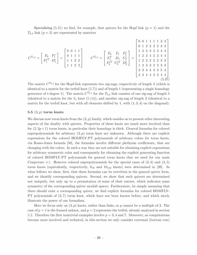
Specializing (5.31) we find, for example, that quivers for the Hopf link (p = 1) and the

T2,4 link (p = 2) are represented by matrices

CT2,2 =

[F0 F e1F eT1 De

1

]=

0 0 1 1

0 1 1 1

1 1 3 2

1 1 2 2

CT2,4 =

F0 F1 F e2F T1 D1 U e2F eT2 U eT2 De

2

=

0 0 1 1 1 1 3 3

0 1 2 2 2 2 3 3

1 2 3 3 2 3 4 4

1 2 3 4 2 3 4 4

1 2 2 2 2 2 3 3

1 2 3 3 2 3 3 3

3 3 4 4 3 3 5 4

3 3 4 4 3 3 4 4

(5.37)

The matrix CT2,2 for the Hopf-link represents two zig-zags, respectively of length 3 (which is

identical to a matrix for the trefoil knot (5.7)) and of length 1 (representing a single homology

generator of t-degree 1). The matrix CT2,4 for the T2,4 link consists of one zig-zag of length 5

(identical to a matrix for the 51 knot (5.14)), and another zig-zag of length 3 (identical to a

matrix for the trefoil knot, but with all elements shifted by 1, with (1, 3, 4) on the diagonal).

5.5 (3, p) torus knots

We discuss now torus knots from the (3, p) family, which enables us to present other interesting

aspects of the duality with quivers. Properties of these knots are much more involved than

for (2, 2p+ 1) torus knots, in particular their homology is thick. General formulas for colored

superpolynomials for arbitrary (3, p) torus knot are unknown. Although there are explicit

expressions for the colored HOMFLY-PT polynomials of arbitrary colors for torus knots,

via Rosso-Jones formula [50], the formulas involve different plethysm coefficients, that are

changing with the colors. In such a way they are not suitable for obtaining explicit expressions

for arbitrary symmetric color and consequently for obtaining the explicit generating function

of colored HOMFLY-PT polynomials for general torus knots that we need for our main

Conjecture 4.1. However colored superpolynomials for the special cases of (3, 4) and (3, 5)

torus knots (equivalently, respectively, 819 and 10124 knots) were determined in [39]. In

what follows we show, first, that these formulas can be rewritten in the general quiver form,

and we identify corresponding quivers. Second, we show that such quivers are determined

not uniquely, but only up to a permutation of some of their entries, which indicates some

symmetry of the corresponding quiver moduli spaces. Furthermore, by simply assuming that

there should exist a corresponding quiver, we find explicit formulas for colored HOMFLY-

PT polynomials of (3, 7) torus knot, which have not been known before, and which nicely

illustrate the power of our formalism.

Here we focus only on (3, p) knots, rather than links, so p cannot be a multiple of 3. The

case of p = 1 is the framed unknot, and p = 2 represents the trefoil, already analyzed in section

5.2. Therefore the first nontrivial examples involve p = 3, 4 and 7. Moreover, as computations

become more involved and technical, in this section we only consider extremal (bottom row)

– 29 –

invariants (4.4); with some patience, and taking advantage of structural properties presented

in Conjecture 4.3, these results can be generalized to the full a-dependence.

Let us consider the (3, 4) torus knot first. Its quadruply-graded Poincare polynomial

determined in [39] reads

Pr(a,Q, tr, tc) = a6rQ6rt6r2

c t6rr

r∑α=0

r∑β=α

r∑γ=β

r∑j=γ

a2(j−γ)

[β

α

]t−2c

[γ

β

]t−2c

[j

γ

]t−2c

[r

j

]t−2c

×

×Q−4α−4β+4γ−8jt−2(α2+β2+γ2)−2(j−γ)(α+β+γ)−(j−γ)2

c t−2(α+β+γ)−(j−γ)r × (5.38)

×(− Q2

a2trtc; tc−2)j−γ

(− a2Q2t3rt

2r+1c ; t2c

)j,

where now we denote[βα

]t−2c

=(t−2c ;t−2

c )β(t−2c ;t−2

c )α(t−2c ;t−2

c )β−α. Upon the identification of variables (2.19),

and extracting the terms at the lowest powers of a, we find that that extremal (bottom row)

colored HOMFLY-PT polynomials for the (3, 4) torus knot take form

P bottomr (q) = q6r2r∑

α=0

r∑β=α

r∑γ=β

r∑j=γ

(q2; q2)r q−2α(β−γ+j+1)−2β(j+1)+2γ−2j(r+2)

(q2; q2)α(q2; q2)β−α(q2; q2)γ−β(q2; q2)j−γ(q2; q2)r−j, (5.39)

while its uncolored HOMFLY-PT homology has 5 generators in the bottom row, whose q-

degrees and t-degrees are

(q1, q2, q3, q4, q5) = (−6,−2, 0, 2, 6),

(t1, t2, t3, t4, t5) = (0, 2, 4, 6, 8).(5.40)

Manipulating the expression (5.39) we find that the corresponding quiver is represented by

the following matrix

CT3,4 =

0 1 2 3 5

1 2 3 3 5

2 3 4 4 5

3 3 4 4 5

5 5 5 5 6

(5.41)

This quiver, together with q-degrees and t-degrees of 5 bottom row generators in (5.40),

encode all extremal (bottom row) colored HOMFLY-PT polynomials for the (3, 4) torus

knot, which can be reconstructed from (4.4). Moreover, simply the fact that we are able to

identify this quiver proves the LMOV conjecture for all symmetric representations for this

knot. Furthermore, the matrix CT3,4 captures the structure of the bottom row generators of

HOMFLY-PT homology for the (3, 4) torus knot, which consists of one zig-zag (the same as

for the (2, 7) torus knot) and one diamond. The part of the matrix with (0, 2, 4, 6) on the

diagonal represents the bottom row of the zig-zag, and an additional 4 on the diagonal is the

bottom row of the diamond (4.8).

– 30 –

The next knot in this series is the (3, 5) torus knot. Its HOMFLY-PT homology and

colored superpolynomials were also considered in [39]. For brevity, we just recall that colored

superpolynomials for this knot take form

Pr(a, q, t) =

r∑j=0

j∑k1=0

k1∑k2=0

k2∑k3=0

k3∑k4=0

r−j∑i=0

a8r

(t

q

)2(i+2j−k1−k2−k3−k4+2r)

× (5.42)

× q−2(k1k2+k2k3+k3k4+2(k1+k2+k3+k4)+r+(k1+k2+k3+k4)r−2r2−i(2+k1+r)−j(5+k2+k3+k4+2r)×

×[j

k1

][k1

k2

][k2

k3

][k3

k4

][r − ji

](−a2tq−2; q2)r−j(−a2q−2−2j+2r; q2)k4−j(−a2q2rt3; q2)r−j .

Setting t = −1 and extracting coefficients of minimal powers of a reveals the form of extremal

(bottom row) colored HOMFLY-PT polynomials

P bottomr (q) =

r∑j=0

j∑k1=0

k1∑k2=0

k2∑k3=0

k3∑k4=0

r−j∑i=0

(q2; q2)r× (5.43)

× q−2(k2+k3+k4)−2(k1+k1k2+k2k3+k3k4)−6r−2(k1+k2+k3+k4)r+4r2+2i(1+k1+r)+2j(3+k2+k3+k4+2r)

(q2; q2)i(q2; q2)j−k1(q2; q2)k1−k2(q2; q2)k2−k3(q2; q2)k3−k4(q2; q2)k4(q2; q2)r−j−i.

Furthermore, the HOMFLY-PT homology for (3, 5) torus knot has 7 generators in the bottom

row, with the following q-degrees and t-degrees

(q1, q2, . . . , q7) = (−8,−4,−2, 0, 2, 4, 8),

(t1, t2, . . . , t7) = (0, 2, 4, 4, 6, 6, 8).(5.44)

Manipulating the above expressions we find, surprisingly, that there are two quivers which re-

produce the same extremal (bottom row) colored HOMFLY-PT polynomials via (4.4). These

two quivers are very similar, and their matrices differ only by a permutation of a few entries.

They take the following form; the permuted entries are underlined in the second matrix

CT3,5 =

0 1 2 3 4 5 7

1 2 3 3 5 5 7

2 3 4 4 5 5 7

3 3 4 4 6 5 7

4 5 5 6 6 6 7

5 5 5 5 6 6 7

7 7 7 7 7 7 8

CT3,5 =

0 1 2 3 4 5 7

1 2 3 3 5 5 7

2 3 4 4 5 5 6

3 3 4 4 6 5 7

4 5 5 6 6 7 7

5 5 5 5 7 6 7

7 7 6 7 7 7 8

(5.45)

Again let us stress, that the quiver represented by either of the above matrcies, together with

q-degrees and t-degrees in (5.44), encode all extremal colored HOMFLY-PT polynomials for

(3, 5) torus knot, which can be reconstructed from (4.4). The fact that we are able to identify

these quivers also proves the LMOV conjecture for all symmetric representations for this knot.

The next knot we consider is the (3, 7) torus knot. Its colored superpolynomials, or even

explicit, closed-form expressions of HOMFLY-PT polynomials colored by arbitrary symmet-

ric representations, have not been known before. However, based on the structure (4.4),

– 31 –

and by comparing the results with the Rosso-Jones formula for the first several symmetric

representations, we are able to reconstruct the corresponding quiver, which then encodes

HOMFLY-PT polynomials colored by arbitrary symmetric representations, and correspond-

ing integral LMOV invariants. The homology of the bottom row of the (3, 7) torus knot has

12 generators with the following q-degrees and t-degrees

(q1, q2, . . . , q12) = (−12,−8,−6,−4,−2, 0, 0, 2, 4, 6, 8, 12),

(t1, t2, . . . , t12) = (0, 2, 4, 4, 6, 6, 8, 8, 8, 10, 10, 12),(5.46)

and we find that the corresponding quiver is encoded in a matrix

CT3,7 =

0 1 2 3 4 5 5 6 7 8 9 11

1 2 3 3 5 5 6 7 7 9 9 11

2 3 4 4 5 6 6 7 8 9 10 11

3 3 4 4 5 5 7 7 7 9 9 11

4 5 5 5 6 6 7 7 8 9 10 11

5 5 6 5 6 6 8 7 7 9 9 11

5 6 6 7 7 8 8 8 9 9 10 11

6 7 7 7 7 7 8 8 8 9 10 11

7 7 8 7 8 7 9 8 8 9 9 11

8 9 9 9 9 9 9 9 9 10 10 11

9 9 10 9 10 9 10 10 9 10 10 11

11 11 11 11 11 11 11 11 11 11 11 12

. (5.47)

In this case we also find other quivers, whose matrices differ from the above one by permuta-

tion of several entries, and yet encode the same generating series (4.4).

5.6 Twist knots 41, 61, 81, . . .

Another infinite family of knots that we consider are twist knots, which are labelled by

an integer p. Negative values of this parameter, i.e. p = −1,−2,−3, . . . , correspond to

41, 61, 81, . . . knots; these are simply (2|p|+ 2)1 knots, which are also denoted TK2|p|+2. The

colored HOMFLY-PT polynomials for these knots are determined in [48, 51] and they take

the form

PTK2|p|+2r (a, q) =

∑0≤k|p|≤...≤k2≤k1≤r

[r

k1

][k1

k2

]· · ·[k|p|−1

k|p|

]×

× a2∑|p|i=1 kiq2

∑|p|i=1(k

2i−ki)(a−2q2; q−2)k1(a−2q−2r; q−2)k1 . (5.48)

Following manipulations similar to the previous examples, we find that the quiver correspond-

– 32 –

ing to a given p < 0, i.e. to a given TK2|p|+2 knot, is encoded in the matrix

CTK2|p|+2 =

F0 F F F · · · F F

F T D1 R1 R1 · · · R1 R1

F T RT1 D2 R2 · · · R2 R2

F T RT1 RT2 D3 · · · R3 R3

......

......

. . ....

...

F T RT1 RT2 RT3 · · · D|p|−1 R|p|−1

F T RT1 RT2 RT3 · · · RT|p|−1 D|p|

(5.49)

where

F0 = [0] F =[

0 −1 0 −1]

(5.50)

and

Dk =

2k 2k − 2 2k − 1 2k − 3

2k − 2 2k − 3 2k − 2 2k − 4

2k − 1 2k − 2 2k − 1 2k − 3

2k − 3 2k − 4 2k − 3 2k − 4

Rk =

2k 2k − 2 2k − 1 2k − 3

2k − 1 2k − 3 2k − 2 2k − 4

2k 2k − 1 2k − 1 2k − 3

2k − 2 2k − 3 2k − 2 2k − 4

(5.51)

The element F0 represents a zig-zag of length 1, corresponding to a single homology generator,

while the diagonal blocks Dk represent (up to a permutation of homology generators, and

an overall shift) diamonds (4.8). Note that in this case it also makes sense to consider the

−p→∞ limit, and the corresponding infinite quiver.

The other parameters that determine the form of the generating series (4.1) for the

TK2|p|+2 knot take the form

(−1)∑i pidi = (−1)(d3+d4)+(d7+d8)+...+(d4|p|−1+d4|p|)+2(d5+d9+...+d4|p|+1),∑

i

aidi = 2d2 + 0d3 + 0d4 − 2d5+

+ 4d6 + 2d7 + 2d8 + 0d9+ (5.52)

...

+ 2|p|d4|p|−2 + (2|p| − 2) d4|p|−1 + (2|p| − 2) d4|p| + (2|p| − 4) d4|p|+1,∑i

lidi = −2d2 − d3 + d4 + 2d5+

− 4d6 − 3d7 − 1d8 + 0d9+

... (5.53)

− 2|p|d4|p|−2 + (1− 2|p|) d4|p|−1 + (3− 2|p|) d4|p| + (4− 2|p|) d4|p|+1.

– 33 –

For example, the quiver for the p = −1 case, i.e. the figure-eight knot 41, whose homology

diagram is shown in figure 2, is represented by the matrix

CTK4 =

[F0 F

F T D1

]=

0 0 −1 0 −1

0 2 0 1 −1

−1 0 −1 0 −2

0 1 0 1 −1

−1 −1 −2 −1 −2

(5.54)

This matrix is consistent with Conjecture 4.3: the top left entry 0 represents the zig-zag of

length 1, and the remaining diagonal block of size 4× 4 represents a diamond and agrees (up

to a permutation of homology generators, and corresponding rows and columns) with (4.8)

for k = −2.

For p = −2, i.e. the 61 knot, the quiver is represented by the following matrix

CTK6 =

F0 F F

F T D1 R1

F T RT1 D2

=

0 0 −1 0 −1 0 −1 0 −1

0 2 0 1 −1 2 0 1 −1

−1 0 −1 0 −2 1 −1 0 −2

0 1 0 1 −1 2 1 1 −1

−1 −1 −2 −1 −2 0 −1 0 −2

0 2 1 2 0 4 2 3 1

−1 0 −1 1 −1 2 1 2 0

0 1 0 1 0 3 2 3 1

−1 −1 −2 −1 −2 1 0 1 0

(5.55)

Note that in these examples some entries of matrices C are negative. In order to have a

proper quiver representation theory interpretation, we can change the framing (4.7) to shift

all values of these matrices by a constant and make them nonnegative.

5.7 Twist knots 31, 52, 72, 92, . . .

Another class of twist knots is characterized by p > 0, which are respectively 31, 52, 72, 92, . . .

knots, which have 2p + 1 crossings, and are also denoted TK2p+1. Their superpolynomials

take the form [51]

PTK2p+1

Sn−1 (a, q, t) =∑

0≤s1≤...≤sp<∞(−t)−n+1q2sp

(−a2tq−2; q2)sp(q2; q2)sp

(q2−2n; q2)sp(−a2t3q2n−2; q2)sp×

×p−1∏i=1

q4si(a2t2)siq2si(si−1)

[si+1

si

]. (5.56)

Here we can illustrate another subtlety, which is the fact that sometimes – in particular

for TK2p+1 knots – more general quivers can be assigned to a given knot, which are however

– 34 –

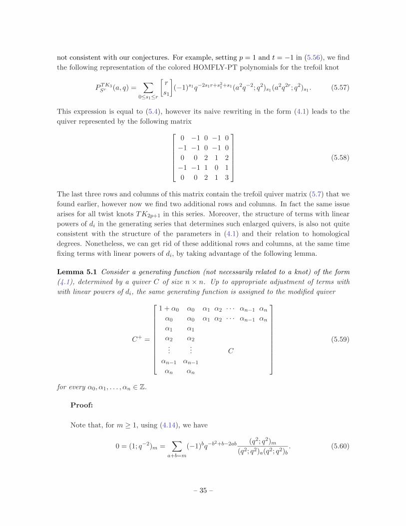
not consistent with our conjectures. For example, setting p = 1 and t = −1 in (5.56), we find

the following representation of the colored HOMFLY-PT polynomials for the trefoil knot

P TK3Sr (a, q) =

∑0≤s1≤r

[r

s1

](−1)s1q−2s1r+s21+s1(a2q−2; q2)s1(a2q2r; q2)s1 . (5.57)

This expression is equal to (5.4), however its naive rewriting in the form (4.1) leads to the

quiver represented by the following matrix0 −1 0 −1 0

−1 −1 0 −1 0

0 0 2 1 2

−1 −1 1 0 1

0 0 2 1 3

(5.58)

The last three rows and columns of this matrix contain the trefoil quiver matrix (5.7) that we

found earlier, however now we find two additional rows and columns. In fact the same issue

arises for all twist knots TK2p+1 in this series. Moreover, the structure of terms with linear

powers of di in the generating series that determines such enlarged quivers, is also not quite

consistent with the structure of the parameters in (4.1) and their relation to homological

degrees. Nonetheless, we can get rid of these additional rows and columns, at the same time

fixing terms with linear powers of di, by taking advantage of the following lemma.

Lemma 5.1 Consider a generating function (not necessarily related to a knot) of the form

(4.1), determined by a quiver C of size n × n. Up to appropriate adjustment of terms with

with linear powers of di, the same generating function is assigned to the modified quiver

C+ =

1 + α0 α0 α1 α2 · · · αn−1 αnα0 α0 α1 α2 · · · αn−1 αnα1 α1

α2 α2

...... C

αn−1 αn−1

αn αn

(5.59)

for every α0, α1, . . . , αn ∈ Z.

Proof:

Note that, for m ≥ 1, using (4.14), we have

0 = (1; q−2)m =∑

a+b=m

(−1)bq−b2+b−2ab (q2; q2)m

(q2; q2)a(q2; q2)b. (5.60)

– 35 –

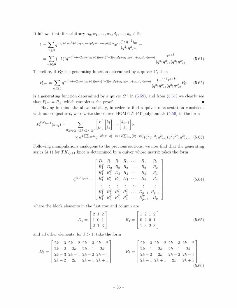
It follows that, for arbitrary α0, α1, . . . , αn, d1, . . . , dn ∈ Z,

1 =∑m≥0

q(α0+1)m2+2(α1d1+α2d2+...+αndn)mxm(1; q−2)m(q2; q2)m

=

=∑a,b≥0

(−1)bq−b2+b−2ab+(α0+1)(a+b)2+2(α1d1+α2d2+...+αndn)(a+b) xa+b

(q2; q2)a(q2; q2)b. (5.61)

Therefore, if PC is a generating function determined by a quiver C, then

PC+ =∑a,b≥0

q−b2+b−2ab+(α0+1)(a+b)2+2(α1d1+α2d2+...+αndn)(a+b) (−1)bxa+b

(q2; q2)a(q2; q2)bPC (5.62)

is a generating function determined by a quiver C+ in (5.59), and from (5.61) we clearly see

that PC+ = PC , which completes the proof.

Having in mind the above subtlety, in order to find a quiver representation consistent

with our conjectures, we rewrite the colored HOMFLY-PT polynomials (5.56) in the form

PTK2p+1r (a, q) =

∑0≤kp≤...≤k2≤k1≤r

[r

k1

][k1

k2

]· · ·[kp−1

kp

]×

× a2∑pi=2 kiq−2k1r+k21+k1+2

∑pi=2(k

2i−ki)(a2q−2; q2)k1(a2q2r; q2)k1 . (5.63)

Following manipulations analogous to the previous sections, we now find that the generating

series (4.1) for TK2p+1 knot is determined by a quiver whose matrix takes the form

CTK2p+1 =

D1 R1 R1 R1 · · · R1 R1

RT1 D2 R2 R2 · · · R2 R2

RT1 RT2 D3 R3 · · · R3 R3

RT1 RT2 RT3 D4 · · · R4 R4

......

......

. . ....

...

RT1 RT2 RT3 RT4 · · · Dp−1 Rp−1

RT1 RT2 RT3 RT4 · · · RTp−1 Dp

(5.64)

where the block elements in the first row and column are

D1 =

2 1 2

1 0 1

2 1 3

R1 =

1 2 1 2

0 2 0 1

1 3 2 3

(5.65)

and all other elements, for k > 1, take the form

Dk =

2k − 3 2k − 2 2k − 3 2k − 2

2k − 2 2k 2k − 1 2k

2k − 3 2k − 1 2k − 2 2k − 1

2k − 2 2k 2k − 1 2k + 1

Rk =

2k − 3 2k − 2 2k − 3 2k − 2

2k − 1 2k 2k − 1 2k

2k − 2 2k 2k − 2 2k − 1

2k − 1 2k + 1 2k 2k + 1

(5.66)

– 36 –

In this case D1 represents a zig-zag of the same form as for the trefoil knot (5.7), and the Dk

(for k > 1) represent (up to a permutation of homology generators and an overall constant

shift) the diamonds (4.8).

The other parameters that determine (4.1), now with vertices of a quiver (or homology

generators), and thus also the summation variables di numbered from 3 to 4p + 1 (after

removing d1 and d2 using the above lemma), take the form

(−1)∑4p+1i=3 tidi = (−1)(d3+d4)+(d7+d8)+...+(d4p−1+d4p)+2(d5+d9+...+d4p+1)

4p+1∑i=3

aidi = 2(d3 + d4) + 4d5+

+ 2d6 + 4d7 + 4d8 + 6d9+ (5.67)

+ 4d10 + 6d11 + 6d12 + 8d13+

...

+ 2(p− 1)d4p−2 + 2pd4p−1 + 2pd4p + 2(p+ 1)d4p+1

4p∑i=2

lidi = −2d4 − 3d5+

− d6 − 2d7 − 4d8 − 5d9+

− 3d10 − 4d11 − 6d12 − 7d13+

... (5.68)

+ (1− 2p)d4p−2 + (2− 2p)d4p−1 + (−2p)d4p + (−1− 2p)d4p+1.

For example, for p = 1, which represents simply the trefoil knot, the quiver matrix (5.64)

consists only of the element D1 in (5.65), and up to permutation of vertices it is equivalent

to (5.7). For p = 2, i.e. for the knot 52, from (5.64) we obtain a quiver represented by the

matrix

CTK5 =

D1 R1 R1

RT1 D2 R2

RT1 RT2 D3

=

2 1 2 1 2 1 2

1 0 1 0 2 0 1

2 1 3 1 3 2 3

1 0 1 1 2 1 2

2 2 3 2 4 3 4

1 0 2 1 3 2 3

2 1 3 2 4 3 5

(5.69)

5.8 62 and 63 knots

Finally we discuss knots with six crossings, 62 and 63 (the third prime knot with six crossings

is the twist knot 61, whose quiver we already identified in (5.55)). Explicit expressions for

colored polynomials for those knots have not been known before. Assuming that they are

– 37 –

consistent with our conjectures, we are able to determine such expressions, as being encoded

in the corresponding quivers. This again shows the power of our formalism.

Let us consider 62 knot first. Its uncolored HOMFLY-PT homology has 11 generators,

which have the following degrees

(a1, . . . , a11) = (0, 2, 2, 0, 2, 2, 2, 4, 4, 2, 4),

(q1, . . . , q11) = (−2,−4,−2, 2, 0, 0, 2,−2, 0, 4, 2),

(t1, . . . , t11) = (−2,−1, 0, 0, 1, 1, 2, 2, 3, 3, 4).

(5.70)

Assuming that the generating series of colored HOMFLY-PT polynomials takes the form (4.1),

and comparing that generating series with several first such polynomials obtained using the

Rosso-Jones formula, we find that the corresponding quiver is encoded in the following matrix

C62 =

−2 −2 −1 −1 −1 −1 0 −1 1 1 1

−2 −1 −1 0 0 0 1 0 1 2 2

−1 −1 0 1 0 0 1 0 1 2 2

−1 0 1 0 0 0 1 0 2 1 1

−1 0 0 0 1 1 1 1 2 2 2

−1 0 0 0 1 1 1 1 2 2 2

0 1 1 1 1 1 2 1 2 2 2

−1 0 0 0 1 1 1 2 2 3 3

1 1 1 2 2 2 2 2 3 3 3

1 2 2 1 2 2 2 3 3 3 3

1 2 2 1 2 2 2 3 3 3 4

(5.71)

In this matrix one can identify diagonal blocks, one corresponding to a zig-zag of the same

form as in the trefoil quiver (5.7), and two diamonds of the form (4.8).

Analogously we analyze the generating series for the 63 knot, whose uncolored HOMFLY-

PT homology has 13 generators of the following degrees

(a1, . . . , a13) = (0, 2, 0, 0,−2, 2, 0, 0,−2, 2, 0, 0,−2),

(q1, . . . , q13) = (0,−2, 0,−4,−2, 0, 2,−2, 0, 2, 4, 0, 2),

(t1, . . . , t13) = (0, 1, 0,−2,−3, 2, 1,−1,−2, 3, 2, 0,−1).

(5.72)

Similarly, comparing first few colored HOMFLY-PT polynomials from (4.1) with the Rosso-

– 38 –

Jones formula, we find the corresponding quiver

C63 =

0 0 0 −1 −1 0 0 −1 −1 0 0 −1 −1

0 1 0 −1 −2 1 0 −1 −2 1 1 0 −1

0 0 0 −1 −2 1 0 0 −2 1 1 0 0

−1 −1 −1 −2 −3 0 −1 −2 −3 −1 0 −2 −2

−1 −2 −2 −3 −3 −1 −1 −2 −3 −1 −1 −2 −2

0 1 1 0 −1 2 1 0 −1 2 1 1 −1

0 0 0 −1 −1 1 1 0 −1 2 1 1 0

−1 −1 0 −2 −2 0 0 −1 −2 0 0 −1 −2

−1 −2 −2 −3 −3 −1 −1 −2 −2 0 −1 −1 −2

0 1 1 −1 −1 2 2 0 0 3 2 1 0

0 1 1 0 −1 1 1 0 −1 2 2 1 0

−1 0 0 −2 −2 1 1 −1 −1 1 1 0 −1

−1 −1 0 −2 −2 −1 0 −2 −2 0 0 −1 −1

(5.73)

In this matrix one can identify diagonal blocks, one corresponding to a zig-zag of length 1

(representing a homology generator with t-degree 0), and three diamonds of the form (4.8).

We checked that the above results agree with those obtained using the formalism of

differentials, presented in [52].

Acknowledgments

We thank Sergei Gukov, Satoshi Nawata, Mi losz Panfil, Yan Soibelman, Richard Thomas,

Cumrun Vafa, and Paul Wedrich for comments and discussions. We are grateful to the

American Institute of Mathematics (San Jose), the Isaac Newton Institute for Mathematical

Sciences (Cambridge University), and Institut Henri Poincare (Paris) for hospitality. The

last author thanks the California Institute of Technology, the Matrix Institute (University

of Melbourne, Creswick), University of California Davis, and the Isaac Newton Institute for

Mathematical Sciences (Cambridge University) for hospitality and opportunity to present the

results of this work during seminars and conferences within the last year. This work is sup-

ported by the ERC Starting Grant no. 335739 “Quantum fields and knot homologies” funded

by the European Research Council under the European Unions Seventh Framework Pro-

gramme, and the Foundation for Polish Science. M.S. is partially supported by the Ministry

of Science of Serbia, project no. 174012.

– 39 –

References

[1] P. Kucharski, M. Reineke, M. Stosic and P. Sulkowski, BPS states, knots and quivers,

1707.02991.

[2] H. Ooguri and C. Vafa, Knot invariants and topological strings, Nucl.Phys. B577 (2000)

419–438, [hep-th/9912123].

[3] J. M. F. Labastida and M. Marino, Polynomial invariants for torus knots and topological

strings, Commun. Math. Phys. 217 (2001) 423–449, [hep-th/0004196].

[4] J. M. F. Labastida, M. Marino and C. Vafa, Knots, links and branes at large N, JHEP 11

(2000) 007, [hep-th/0010102].

[5] E. Witten, Chern-Simons gauge theory as a string theory, Prog. Math. 133 (1995) 637–678,

[hep-th/9207094].

[6] E. Witten, Quantum field theory and the Jones polynomial, Comm. Math. Phys. 121 (1989)

351–399.

[7] P. Ramadevi and T. Sarkar, On link invariants and topological string amplitudes, Nucl. Phys.

B600 (2001) 487–511, [hep-th/0009188].

[8] A. Mironov, A. Morozov, A. Morozov, P. Ramadevi, V. K. Singh and A. Sleptsov, Checks of

integrality properties in topological strings, 1702.06316.

[9] S. Garoufalidis, P. Kucharski and P. Sulkowski, Knots, BPS states, and algebraic curves,

Commun. Math. Phys. 346 (2016) 75–113, [1504.06327].

[10] P. Kucharski and P. Sulkowski, BPS counting for knots and combinatorics on words, JHEP 11

(2016) 120, [1608.06600].

[11] W. Luo and S. Zhu, Integrality structures in topological strings I: framed unknot, 1611.06506.

[12] S. Zhu, Topological strings, quiver varieties and Rogers-Ramanujan identities, 1707.00831.

[13] M. Kontsevich and Y. Soibelman, Stability structures, motivic Donaldson-Thomas invariants

and cluster transformations, 0811.2435.

[14] M. Kontsevich and Y. Soibelman, Cohomological Hall algebra, exponential Hodge structures and

motivic Donaldson-Thomas invariants, Commun. Num. Theor. Phys. 5 (2011) 231–352,

[1006.2706].

[15] M. Reineke, Cohomology of quiver moduli, functional equations, and integrality of

donaldsonthomas type invariants, Compositio Mathematica 147 (5, 2011) 943–964.

[16] M. Reineke, Degenerate Cohomological Hall algebra and quantized Donaldson-Thomas

invariants for m-loop quivers, Doc. Math. 17 (2012) 1, [1102.3978].

[17] J. A. Harvey and G. W. Moore, On the algebras of BPS states, Commun. Math. Phys. 197

(1998) 489–519, [hep-th/9609017].

[18] A. I. Efimov, Cohomological hall algebra of a symmetric quiver, Compositio Mathematica 148

(2012) 1133–1146.

[19] S. Meinhardt and M. Reineke, Donaldson-Thomas invariants versus intersection cohomology of

quiver moduli, 1411.4062.

– 40 –

[20] H. Franzen and M. Reineke, Semi-Stable Chow-Hall Algebras of Quivers and Quantized

Donaldson-Thomas Invariants, 1512.03748.

[21] M. Aganagic and C. Vafa, Large n duality, mirror symmetry, and a q-deformed a-polynomial for

knots, 1204.4709.

[22] W. Nahm, Conformal field theory and torsion elements of the Bloch group, hep-th/0404120.

[23] S. Garoufalidis and T. T. Le, Nahm sums, stability and the colored jones polynomial, Research

in the Mathematical Sciences 2 (2015) 1.

[24] D.-E. Diaconescu, Z. Hua and Y. Soibelman, HOMFLY polynomials, stable pairs and motivic

Donaldson-Thomas invariants, 1202.4651.

[25] A. Schwarz, V. Vologodsky and J. Walcher, Framing the Di-Logarithm (over Z), Proc. Symp.

Pure Math. 90 (2015) 113–128, [1306.4298].

[26] A. Schwarz, V. Vologodsky and J. Walcher, Integrality of Framing and Geometric Origin of

2-functions, 1702.07135.

[27] M. Dedushenko and E. Witten, Some Details On The Gopakumar-Vafa and Ooguri-Vafa

Formulas, Adv. Theor. Math. Phys. 20 (2016) 1–133, [1411.7108].

[28] M. Kameyama and S. Nawata, Refined large N duality for knots, 1703.05408.

[29] J. M. F. Labastida and M. Marino, A new point of view in the theory of knot and link

invariants, J. Knot Theory Ramifications 11 (2002) 173–197, [math/0104180].

[30] K. Liu and P. Peng, Proof of the Labastida-Mario-Ooguri-Vafa conjecture, J. Diff. Geom. 85

(2010) 479–525, [0704.1526].

[31] M. Khovanov, A categorification of the Jones polynomial, Duke Math. J. 101 (2000) 359426,

[math/9908171].

[32] M. Khovanov and L. Rozansky, Matrix factorizations and link homology, Fund. Math. 199

(2008) 1–91, [math/0401268].

[33] M. Khovanov and L. Rozansky, Matrix factorizations and link homology II, Geom. & Topol. 12

(2008) 1387–1425, [math/0505056].

[34] S. Cautis, Remarks on coloured triply graded link invariants, 1611.09924.

[35] P. Wedrich, Exponential growth of colored HOMFLY-PT homology, 1602.02769.

[36] N. M. Dunfield, S. Gukov and J. Rasmussen, The superpolynomial for knot homologies,

Experiment. Math. 15 (2006) 129–159, [math/0505662].

[37] J. Rasmussen, Some differentials on Khovanov-Rozansky homology, Geom. Topol. 19 (2010)

3031–3104, [math/0607544].

[38] S. Gukov and M. Stosic, Homological Algebra of Knots and BPS States, Proc. Symp. Pure Math.

85 (2012) 125–172, [1112.0030].

[39] S. Gukov, S. Nawata, I. Saberi, M. Stosic and P. Sulkowski, Sequencing BPS Spectra, JHEP 03

(2016) 004, [1512.07883].

[40] S. Gukov, A. Schwarz and C. Vafa, Khovanov-rozansky homology and topological strings, Lett.

Math. Phys. 74 (2005) 53–74, [hep-th/0412243].

– 41 –

[41] S. Gukov, A. Iqbal, C. Kozcaz and C. Vafa, Link Homologies and the Refined Topological

Vertex, Commun. Math. Phys. 298 (2010) 757–785, [0705.1368].

[42] M. Aganagic and S. Shakirov, Knot Homology and Refined Chern-Simons Index, Commun.

Math. Phys. 333 (2015) 187–228, [1105.5117].

[43] H. Awata, S. Gukov, P. Sulkowski and H. Fuji, Volume Conjecture: Refined and Categorified,

Adv. Theor. Math. Phys. 16 (2012) 1669–1777, [1203.2182].

[44] P. Dunin-Barkowski, A. Mironov, A. Morozov, A. Sleptsov and A. Smirnov, Superpolynomials

for toric knots from evolution induced by cut-and-join operators, JHEP 03 (2013) 021,

[1106.4305].

[45] H. Fuji, S. Gukov and P. Sulkowski, Super-A-polynomial for knots and BPS states, Nucl. Phys.

B867 (2013) 506–546, [1205.1515].

[46] H. Itoyama, A. Mironov, A. Morozov and A. Morozov, HOMFLY and superpolynomials for

figure eight knot in all symmetric and antisymmetric representations, JHEP 07 (2012) 131,

[1203.5978].

[47] E. Gorsky, S. Gukov and M. Stosic, Quadruply-graded colored homology of knots, 1304.3481.

[48] H. Fuji, S. Gukov, M. Stosic and P. Sulkowski, 3d analogs of Argyres-Douglas theories and knot

homologies, JHEP 01 (2013) 175, [1209.1416].

[49] J. Engel and M. Reineke, Smooth models of quiver moduli, Mathematische Zeitschrift 262

(2009) 817–848.

[50] M. Rosso and J. V., On the invariants of torus knots derived from quantum groups, J. Knot

Theory Ramif. 2 (1993) 97–112.

[51] S. Nawata, P. Ramadevi, Zodinmawia and X. Sun, Super-A-polynomials for Twist Knots, JHEP

11 (2012) 157, [1209.1409].

[52] S. Nawata and A. Oblomkov, Lectures on knot homology, Contemp. Math. 680 (2016) 137,

[1510.01795].

– 42 –