knots and dynamics - École normale supérieure de...

Knots and dynamics

Étienne Ghys

Abstract. The trajectories of a vector field in 3-space can be very entangled; the flow canswirl, spiral, create vortices etc. Periodic orbits define knots whose topology can sometimes bevery complicated. In this talk, I will survey some advances in the qualitative and quantitativedescription of this kind of phenomenon. The first part will be devoted to vorticity, helicity, andasymptotic cycles for flows. The second part will deal with various notions of rotation and spinfor surface diffeomorphisms. Finally, I will describe the important example of the geodesicflow on the modular surface, where the linking between geodesics turns out to be related towell-known arithmetical functions.

Mathematics Subject Classification (2000). Primary 37–02; Secondary 57–02.

Keywords. Low-dimensional dynamical systems, periodic orbits, knots and links.

1. Flows

1.1. Vorticity. Let us start with some historical motivation. Consider a perfect in-compressible fluid moving inside some bounded domain M in 3-space, with no ex-ternal forces. At time t , the velocity is described by a divergence free vector field vt ,tangent to the boundary of M , which evolves in time according to the classical Eulerequation: D

Dtvt (= ∂

∂tvt + vt · ∇vt ) is the (opposite) gradient−∇p of the pressure p.

Denote by φt the associated flow: the trajectory of a particle initially located at x ∈ Mis the curve t �→ φt (x). The curl ωt = ∇×vt is known as the vorticity vector field.One of the earliest results in fluid dynamics is due to H. Helmholtz and W. Kelvin:

The vorticity ωt is merely transported by the flow, i.e. at any time t , one hasωt = dφt (ω0).

This is not difficult to prove: take a closed loop c in M , and compute the timederivative of the circulation of vt along the loop ct = φt (c).

D

Dt

(∮ct

vt · dct)=∮ct

(Dvt

Dt· dct + vt · Ddct

Dt

)

=∮ct

(−∇p · dct + vt · dvt )

=∫ct

d(−p + |vt |2

2) = 0.

Proceedings of the International Congressof Mathematicians, Madrid, Spain, 2006© 2007 European Mathematical Society

248 Étienne Ghys

When c reduces to an infinitesimal loop, Stokes’ formula shows that dφ−t (ωt ) isindeed constant in time.

A much more conceptual proof is due to V. Arnold who realized that Euler’sequation can be seen as the geodesic flow on the infinite dimensional Lie group ofvolume preserving diffeomorphisms of M , equipped with a natural right invariantmetric [3], [5], [55]. This right invariance implies a symmetry group for the equation,which yields Helmoltz–Kelvin’s result as a special case of Noether’s general principlethat symmetries imply conservation laws.

If one can define quantities associated to divergence free vector fields, which areinvariant under conjugacies by volume preserving diffeomorphisms, these quantitiesevaluated on the vorticity ωt will therefore be constants of motion. In this talk, wewill discuss some of these invariants, of topological origin.

One consequence seemed remarkable to W. Kelvin. Suppose that at time 0, thevector field v0 possesses a vortex ring: a solid torus S1 × D embedded in M in sucha way that ω0 is tangent to its boundary. Then, this ring will survive as a vortexring under time evolution, preserving the same topology. This stability of vorticeswas the starting point of the (now forgotten) theory of “vortex atoms”, trying toexplain elementary “atoms” as vortex rings in ether. Even though this turned outto be physically incorrect, it represents one of the first attempts to use topology inphysics. In any case, it motivated P. Tait to start a systematic study of knots, thereforecreating knot theory. See [26] for a fascinating historical survey of this great momentof interaction between physics and mathematics.

A similar phenomenon appeared much more recently in magneto-hydrodynamics:the dynamics of electrically conducting fluids (like a plasma). If one assumes thatthe fluid is perfect and has no resistance (ideal MHD), the magnetic (divergence free)vector field is merely transported by the flow of the fluid [21]. For instance, if twoperiodic orbits of the magnetic field are linked at time t = 0, these orbits will survivefor ever and remain linked. Again, an invariant of divergence free vector fields yieldsconservation laws. See for instance [5], [15].

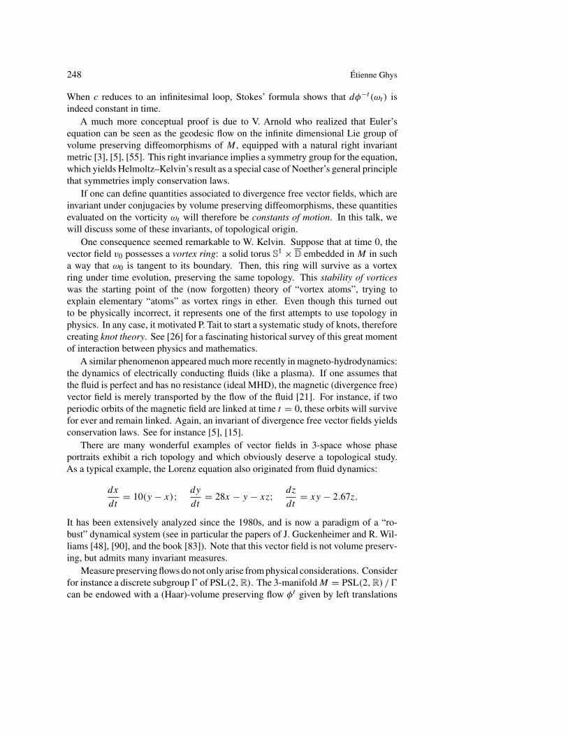
There are many wonderful examples of vector fields in 3-space whose phaseportraits exhibit a rich topology and which obviously deserve a topological study.As a typical example, the Lorenz equation also originated from fluid dynamics:

dx

dt= 10(y − x); dy

dt= 28x − y − xz; dz

dt= xy − 2.67z.

It has been extensively analyzed since the 1980s, and is now a paradigm of a “ro-bust” dynamical system (see in particular the papers of J. Guckenheimer and R. Wil-liams [48], [90], and the book [83]). Note that this vector field is not volume preserv-ing, but admits many invariant measures.

Measure preserving flows do not only arise from physical considerations. Considerfor instance a discrete subgroup� of PSL(2,R). The 3-manifoldM = PSL(2,R) /�can be endowed with a (Haar)-volume preserving flow φt given by left translations

Knots and dynamics 249

Figure 1. The Lorenz attractor.

(xy)2x

trefoil x(yx)3

type (4, 3)torus knot

xy(xy3)2

type (−3,−7, 2)torus knot

Figure 2. Some periodic orbits [17].

by diagonal matrices (exp(t) 0

0 exp(−t)).

The dynamics of this kind of flow has been widely investigated in particular becauseof its strong links with number theory (see for instance [84], [68]). We will comeback to this key example in Section 3.

Finally, a huge source of examples of volume preserving vector fields comes fromthe suspension procedure: any area preserving diffeomorphism f of a surface Syields a volume preserving vector field on the 3-manifold obtained by gluing thetwo boundary components of S × [0, 1] using f . We will discuss these examples inSection 2.

1.2. Knots and periodic orbits. If a vector field in the 3-sphere or in a domain ofR3 has a periodic orbit, this defines a knot whose topology can be used to describe thedynamics. Starting from H. Poincaré one century ago, the quest for periodic orbitshas been rewarding1. Here is a sample of results.

As for the existence question, after a long search around Seifert’s conjecture,K. Kuperberg constructed a jewel. There exists a nonsingular real analytic vectorfield in the 3-sphere with no periodic orbit [59] (see also [44]). Note however thatsuch a vector field is highly nongeneric.

H. Hofer showed that the Reeb vector field of any contact form in the 3-sphere hasat least one periodic orbit [50]. H. Hofer, K. Wysocki and E. Zehnder even showedthat at least one of these orbits is unknotted [51].

In between these two cases, the volume preserving case seems difficult:Does there exist a volume preserving real analytic nonsingular vector field in the

3-sphere with no periodic orbit?G. Kuperberg constructed examples of C1 nonsingular aperiodic volume preserv-

ing vector fields in the 3-sphere, but they are not C2 [58]! K. Kuperberg’s examplesare analytic, but not volume preserving!

1“Elles se sont montrées la seule brèche par où nous puissions pénétrer une place jusqu’ici réputée inabordable”(H. Poincaré).

250 Étienne Ghys

In the opposite direction, there are vector fields in the 3-sphere with plenty ofperiodic orbits. R. Ghrist constructed another jewel: an explicit real analytic vectorfield in the 3-sphere whose periodic orbits represent all (isotopy classes of ) knotsand links! [41]. More recently, J. Etnyre and R. Ghrist even constructed an analyticcontact form whose Reeb vector field has the same property [28].

Some vector fields have many periodic orbits representing many knots, but notall. J. Birman and R. Williams pioneered the subject and studied in great detail thecase of the Lorenz equation. The main tool is Birman–Williams’ template theory. InFigure 3 (extracted from the original paper [17]), one sees a template: an embeddingof a branched surface � in R3, equipped with a semi-flow (ψt )t≥0. The inverselimit � of this semi-flow is the space of full orbits, i.e. curves c : R → � such thatψt(c(s)) = c(s+ t) for all s ∈ R and t ≥ 0. This is a compact space equipped with aflow (ψ t )(t∈R) and an equivariant projection π : �→ � (i.e. π � ψ t = ψt �π ). Onecan embed the abstract space � in a small neighborhood of � in R3 in such a waythat π−1(x) lies in a small neighborhood of x in R3 and that ψ t is induced by somesmooth vector field in R3 preserving �. Any orbit of ψ t stays close to a full orbitof the original semi-flow ψt . This is the geometric Lorenz attractor which has beenshown recently to be conjugate to the original Lorenz attractor by W. Tucker [86].

v u u′ v′

1

0

Figure 3. The Lorenz template. Figure 4. The Ghrist template.

In their seminal paper [17], J. Birman and R. Williams were able to reduce thetopological study of the knots and links which are present in the Lorenz vector field to acombinatorial study on the template. For instance, all Lorenz knots are prime [91], arefibered knots, and have non negative signature. Hence, Lorenz knots are numerous,but very peculiar. See also [34], [52].

Amazingly, Ghrist’s original example of a vector field exhibiting all knots andlinks in the 3-sphere is “almost” the same as the Lorenz template (Figure 4)! See thebeautiful book [42] for more information.

1.3. Asymptotic cycles. Consider a vector fieldv on a compact manifoldM , possiblywith boundary, preserving some probability measureμ, and generating a flow φt . Al-though there might be no periodic orbit,μ-almost every pointx is recurrent (Poincaré’srecurrence theorem): there is a sequence tn→∞ such that φtn(x) converges to x; thelong arc of trajectory from x to φtn(x) is therefore “almost closed”. Choose some aux-iliary generic Riemannian metric onM and, for any point x and time T , consider the


closed loop k(T , x) obtained by concatenation of the arc of trajectory from x to φT (x)and some shortest geodesic from φT (x) to x. Denote by [k(T , x)] ∈ H1(M,R) thehomology class of this loop. In the late 1950s, S. Schwartzman observed (in essence)that the limit S(φ; x) = limT→∞[k(T , x)]/T exists in the first homology groupH1(M,R) for μ-almost every point x, and that this limit is independent of the auxil-iary metric used to close the arcs [82]. The average value S(φ) = ∫

MS(φ; x) dμ is

the Schwartzman asymptotic cycle of the flow. Proofs are variations around Birkhoff’sergodic theorem.

As in the classical ergodic theorem, the actual value of S(φ) can be computed asa space average. For each point x, consider the trajectory γx from x to φ1(x) as ade Rham 1-current on M , whose boundary is the difference between a Dirac mass atφ1(x) and a Dirac mass at x. The integral

∫Mγx dμ(x) is a 1-cycle since the integral

of boundaries vanishes (thanks to the invariance of μ). The homology class of thisSchwartzman cycle is indeed equal to the above limit S(φ).

In other words, a measure preserving flow defines a canonical homology classwhich can be considered as an “infinitely long knot”. Schwartzman’s point of viewhas been greatly generalized by D. Sullivan and W. Thurston among others [85].

1.4. Helicity. A typical application of this kind of ideas has been carried out byV. Arnold [4]. Suppose for simplicity that M is the 3-sphere, and that the measureof periodic orbits is zero. Consider two distinct points x1, x2 in M , and two timesT1, T2 > 0. The two closed loops k(T1, x1) and k(T2, x2) are disjoint for almost everychoice of x1, x2, T1, T2 (at least if the metric is generic), and one can consider theasymptotic behavior of their linking number link(k(T1, x1), k(T2, x2)) as T1 and T2tend to infinity. Again, as a consequence of Birkhoff’s ergodic theorem, V. Arnoldproved that for μ-almost every choice of x1, x2, the limit

link(x1, x2) = limT1,T2→∞

1

T1T2link(k(T1, x1), k(T2, x2))

exists (see also [23], [36], [88]).If μ is a volume form, V. Arnold identified the integral

∫∫M×M

link(x1, x2) dμ(x1) dμ(x2)

that he called the asymptotic Hopf invariant as the helicity, which had been introducedpreviously by J.-J. Moreau [67] and K. Moffatt [62], [63], [64], [65], [66] and thatwe now recall. Since φt preserves a volume form μ, the inner product ivμ is a closed2-form, hence can be written dα for some 1-form α. The helicity Hel(v) is equal tothe integral of α ∧ dα over M (which is easily seen to be independent of the choiceof the primitive α). Note the analogy with the usual definition of Hopf’s invariant formaps from the 3-sphere to the 2-sphere. See also [87] for an interesting definition ofhelicity in the spirit of Witten’s approach to Jones’ polynomial.

252 Étienne Ghys

The helicity Hel(v) defines a quadratic form on the Lie algebra of divergence freevector fields, which is invariant under the adjoint action of smooth volume preservingdiffeomorphisms. V. Arnold suggests that Hel(v) is some “Killing form” for this Liealgebra.

The main open question concerning helicity has been raised by V. Arnold [4]:Suppose two smooth volume preserving flows are conjugate by some volume pre-

serving homeomorphism (which is orientation preserving). Does it follow that thetwo flows have the same helicity?

The qualitative description of helicity as a limit of linking numbers suggests apositive answer, but one should be cautious that a homeomorphism might entanglethe small geodesic arcs that were used to close the trajectories. However, we willsee in Section 2 that helicity is indeed a topological invariant for flows with a crosssection.

Similarly, V. Arnold asked for a definition of helicity for volume preserving topo-logical flows: this problem seems to be wide open.

1.5. Digression: the Gordian space. For almost every point x, the curve k(T , x) isa knot, i.e. has no double point. However, since we are using some auxiliary metricto close the trajectory arc, this knot does depend on the metric. The idea behind theprevious constructions is that these knots are “approximately well defined” when Ttends to infinity. This suggests looking at the space of knots, as a rough metric space,à la Gromov.

Denote by K the (countable) set of (isotopy classes of) knots in 3-space. Thereis a natural Gordian distance dGordian on K that we now define. Given two knotsk0, k1 : S1 ↪→ R3, one considers homotopies (kt )t∈[0,1] : S1 � R3 which connectthe two knots and are such that for each t ∈ [0, 1], the curve kt is an immersionwith at most one double point, this double point being generic (the two local arcsthat intersect have distinct tangents at the intersection). Denote by D((kt )t∈[0,1]) thetotal number of double points of this family of curves. The Gordian distance betweenthe two knots k0 and k1 is the minimum of D((kt )t∈[0,1]) for all such homotopiesconnecting the knots.

The global geometry of this (discrete) metric space is quite intriguing and probablyvery intricate. Note for instance that this space is not locally finite (an infinite numberof knots can be made trivial by allowing one crossing). We propose two kinds of“dual” questions.

One could try to prove (or disprove) that a given metric space (E, d) can beembedded quasi-isometrically in (K, dGordian). Recall that a map u : E → K is aquasi-isometric embedding if there are constants C,C′ > 0 such that

C−1d(x, y)− C′ ≤ dGordian(u(x), u(y)) ≤ Cd(x, y)+ C′

for all x, y. For instance, we proved in [39] that every Euclidean space can beembedded quasi-isometrically in (K, dGordian) and J. Marché showed that a countable


tree such that every vertex has countable valency can also be quasi-isometricallyembedded [61].

Can one embed quasi-isometrically the Poincaré disk (or some higher rank sym-metric space) in the Gordian space?

In a second approach, one could try to find maps I : (K, dGordian) → (E, d)

which are quasi-Lipschitz: d(I (x), I (y)) ≤ CdGordian(x, y) + C′ for some suitablemetric space (E, d). Any such invariant I would be a candidate for an adaptation tovector fields since I (k(T , x))would not be very sensitive to the choice of the auxiliaryRiemannian metric, and the ambiguity could disappear in the asymptotic behavior ofI (k(T , x)) as T tends to infinity. Very few examples of such invariants I seem to beknown. The most trivial one is of course the unknotting number, Gordian distanceto the unknot, but this invariant is hard to compute. Equally hard to compute is thegenus, i.e. the smallest genus of a Seifert surface. A very interesting (and easy tocompute) classical invariant is the signature of knots sign : K → Z which is 2-Lipschitz for elementary reasons, as well as its twisted versions signω, associated tocomplex numbers of modulus 1 (see [37], [38], [39], [53]).

In [37], we consider a measure preserving vector field v in a bounded domain Mof R3, and we prove that the limit sign(v; x) = limT→∞ sign(k(T , x))/T 2 exists foralmost every point x. Its average sign(v) = ∫

Msign(v; x) dμ(x) is the signature of

the vector field. When v is ergodic with respect to the invariant measure, this signaturecoincides (surprisingly?) with (one half of) the helicity.

Some other “new” invariants have this Lipschitz property, like the τ invariant ofP. Ozsváth and Z. Szabó, and the s invariant of J. Rasmussen. Do they lead to newdynamical invariants for flows?

In a similar vein, it would be interesting to get some information on the roughgeometry of the space of (homeomorphism types of ) closed 3-manifolds where thedistance between two manifolds is defined as the minimum number of Morse surgerieswhich are necessary to transform one into the other.

2. Diffeomorphisms of surfaces

Braids are useful to study knots and links mainly because they form a group. In thesame way, surface diffeomorphisms are useful to study flows, and also form a group,so that we can use algebraic tools.

If f is a diffeomorphism of a surface S, its suspension is obtained by identifying(x, 0) and (f (x), 1) in the cylinder S × [0, 1]. The corresponding manifold Sf isequipped with a flow and a cross section on which the first return map is precisely f .If f preserves a measure or an area form, the suspension preserves a natural measureor volume form. In this section, we describe many invariants measuring some kindof twisting in surface diffeomorphisms.

254 Étienne Ghys

2.1. The Calabi homomorphism. Denote by G = Diff(D, ∂D, area) the group ofarea preserving diffeomorphisms (say of class C∞) of the closed disk, which are theidentity near the boundary. E. Calabi defined a homomorphism

C : Diff(D, ∂D, area)→ R

in the following way [19]. Choose a primitive α of the area form in the disk. For eachelement f of G, the form f α − α is closed and is therefore the differential dH of aunique functionH on the disk which is zero near the boundary. Then C(f ) is definedas the integral of H .

There is an intuitive description of Calabi’s homomorphism which is due toA. Fathi(unpublished), expressing it as an “average amount of rotation”. The group G iscontractible. Choose some isotopy (ft )t∈[0,1] connecting f0 = id and f1 = f . Ifx1, x2 are distinct points in the disk, the argument of the nonzero vector ft (x1)−ft (x2)

in R2 \ {(0, 0) } rotates by some angle Angle(f ; x1, x2) when t goes from 0 to 1 (as aunit for angles, we use the full turn). It is easy to see that this definition is independentof the chosen isotopy. It turns out that

C(f ) =∫∫

D×D

Angle(f ; x1, x2) dx1 dx2.

This interpretation enables a proof of topological invariance for Calabi’s invariant [36]:If f and g are two elements of G which are conjugate by some area preserv-

ing homeomorphism h of the disk, which is the identity near the boundary, thenC(f ) = C(g).

Indeed, even though h is not assumed to be smooth, one can define the numberAngle(h; x1, x2), and it is obvious that

Angle(f ; x1, x2)− Angle(g;h(x1), h(x2))

= Angle(h; x1, x2)− Angle(h; f (x1), f (x2)).

Note that Angle(h;−,−) is a continuous function on the complement of the diagonalin D×D, and could be nonintegrable if h is not smooth (there could be an unboundedlocal twist). However, the left hand side of the previous equality is bounded since fand g are assumed to be smooth. As for the right hand side, it is easy to see that itsintegral, which is defined, has to vanish (for instance approximating Angle(h;−,−)by a sequence of bounded functions). Hence C(f ) = C(g).

Observe that Calabi’s definition extends to more general symplectic manifoldson which the symplectic form is exact. However, no analogous interpretation as anaverage rotation is known.

The suspension of a diffeomorphism f in G defines a flow f on a solid torusD × S1. If one embeds this solid torus in R3 in a standard way, one can computethe helicity of the suspended flow. In [36], we proved that this helicity is equal to(an explicit multiple of) Calabi’s invariant of f . (One has to be slightly careful with


definitions in nonsimply connected manifolds, see [36]). This follows rather easilyfrom Fathi’s interpretation of Calabi’s invariant andArnold’s interpretation of helicity.

As a consequence of the topological invariance of Calabi’s number, we get thetopological invariance of helicity for flows which are suspensions of area preservingdiffeomorphisms of the disk. This is a positive answer to a special case of V. Arnold’squestion mentioned above.

2.2. Some algebraic properties of diffeomorphism groups. The kernel of Calabi’shomomorphism C is a simple group [8], [9]. However, the following fundamentalquestion remains open:

Is the group Homeo(D, ∂D, area) of area preserving homeomorphisms of the diskwhich are the identity near the boundary a simple group?

One could try to extend Calabi’s homomorphism to this group of homeomor-phisms, but the obvious idea of using the integral of Angle(h;−,−) does not work!If one assumes some rather low regularity for the homeomorphisms, one can never-theless use this idea, as in the quasi-conformal case [49].

Consider now a closed surface S, equipped with some area form ω (say of totalarea 1), and let Diff0(S, ω) denote the identity component of the group of smooth(say of class C∞) diffeomorphisms preserving ω. The question of the simplicity ofthese groups has been settled in the early 1980s (see [7], [9]).• The group Diff0(S

2, area) of area (and orientation) preserving diffeomorphismsof the 2-sphere is a simple group. As above, the question of the simplicity of thegroup of area preserving homeomorphisms of the sphere is open.• If S is a compact oriented surface of genus at least 2, there is a flux homomor-

phism F : Diff0(S, area)→ H1(S,R) � R2g whose kernel is simple, as proved byA. Banyaga. The definition of F , due to E. Calabi, is in the spirit of Schwartzman [19].Let f ∈ Diff0(S, area), and choose some isotopy (ft )t∈[0,1] connecting the identityto f . For each point x ∈ S, the curve γx : t ∈ [0, 1] �→ ft (x) ∈ S can be consideredas a 1-current, and the integral

∫Sγx d area(x) is a 1-cycle whose homology class

F (f ) is independent of the choice of the isotopy (this follows from the contractibilityof Diff0(S, area)). The kernel of F consists of Hamiltonian diffeomorphisms of S.• Diff0(T

2, area) is not contractible, but retracts to the subgroup of translations,isomorphic to T2. It follows that the flux is well defined on the universal cover or, bet-ter, is defined as a homomorphism F : Diff0(T

2, area)→ H1(T2,R)/H1(T

2,Z) �R2/Z2. Again, the kernel of the flux is the simple group of Hamiltonian diffeomor-phisms of the torus.

Note that these flux homomorphisms can easily be extended to the groups of areapreserving homeomorphisms which are homotopic to the identity. In particular, thesefluxes are invariant under topological area preserving conjugacy.

2.3. Dynamical quasi-morphisms. A map F from a group G to R is a quasi-morphism if |F(g1g2)−F(g1)−F(g2)| is uniformly bounded (see for instance [57]).One says that F is homogeneous if F(gn) = nF(g) for every n ∈ Z and g ∈ G. For

256 Étienne Ghys

every quasi-morphism, the limit F(g) = limn→∞ F(gn)/n exists, and this homoge-nization defines a quasi-morphism such that |F − F | is bounded.

Some quasi-morphisms have a dynamical flavor. Let Homeo(S1) be the universalcover of the group of orientation preserving homeomorphisms of the circle, seenas the group of homeomorphisms of R commuting with integral translations. The

map f ∈ Homeo(S1) �→ f (0) ∈ R is a quasi-morphism whose homogenization isprecisely Poincaré’s rotation number (see for instance [46]).

Given a group G, the existence of quasi-morphisms which are nontrivial (i.e. notat a bounded distance from a homomorphism) is related to the second bounded coho-mology group of G (see [47]). In turn, this is related to the commutator length. If anelement g belongs to the first derived group [G,G], it can be written, by definition, asa product of commutators. Let us denote by comm(g) the smallest length of such aproduct, and set comm(g) = limn→∞ comm(gn)/n. It turns out that nontrivial quasi-morphisms exist if and only if comm does not vanish identically on [G,G] [12]. Forinstance, if � is a nonelementary Gromov hyperbolic group, the space of homoge-neous quasi-morphisms is infinite dimensional [27]. In the opposite direction, if � isa uniform lattice in a simple Lie group of real rank at least 2, then every homogeneousquasi-morphism is trivial: a strong improvement of the now classical vanishing of thefirst Betti number of such lattices [18].

Since we know all homomorphisms from Diff0(S, area) to R (and they are not sonumerous), it is tempting to try to understand nontrivial quasi-morphisms, in the spiritof Poincaré’s rotation number, as an attempt to measure some amount of “twisting”,or “rotation”, or “braiding”, contained in some area preserving diffeomorphism. Inthe next subsections, we will sketch several constructions showing that:

For every closed oriented surface S, the space of homogeneous quasi-morphismsfrom Diff0(S, area) to R is infinite dimensional [38].

Hopefully, such invariants could be numerous enough to provide a precise de-scription of the topological dynamics, as in the case of circle homeomorphisms (seefor instance [46]). As a motivation, let us recall a (generalization of a) conjecture ofR. Zimmer which attracted a lot of attention [93]:

Suppose that a lattice in a simple Lie group of real rank r acts faithfully byhomeomorphisms on some compact manifold M of dimension d. Does it follow thatd ≥ r?

Some very special cases of this conjecture are known to be true:• In dimension d = 1, the conjecture is settled for smooth actions of general

lattices [18], [29], [45], and even for groups with Kazdhan’s property T [69]. It is openfor topological actions of general lattices. It has been proved for topological actionsfor some specific lattices (typically lattices commensurable to SL(n,Z) (n ≥ 3)) [60],[92].• In dimension 2, the conjecture is open in full generality. However, it has been

proved by very different techniques for specific lattices (for instance lattices commen-surable to SL(n,Z) with n ≥ 3) under some additional assumptions: in [32], [33]


for smooth area preserving actions; in [76] for smooth area preserving actions on aclosed oriented surface of genus at least 1; in [43] for real analytic actions on closedsurfaces different from the torus, and in [79] for the torus case.• In higher dimension, not much is known, unless one adds strong conditions on

the action, like assuming that the action preserves a connection [31], or is holomorphicon a Kaehler manifold [20], or for specific lattices acting analytically on 4-manifoldswith non zero Euler–Poincaré characteristic [30] etc.

One of the first nontrivial open cases of this conjecture is the following.Can a uniform lattice in a simple Lie group of real rank at least 2 act faithfully

on a compact surface by area preserving diffeomorphisms?Suppose a group � embeds in Diff0(S, area), and let F be a quasi-morphism

on Diff0(S, area). This produces a quasi-morphism on �. For instance, if � isa uniform lattice in SL(n,R) (n ≥ 3), we already mentioned that such a quasi-morphism has to be trivial. If one could construct a wealth of quasi-morphisms onDiff0(S, area)with strong dynamical content, this vanishing result could lead to strongdynamical restrictions on possible actions of lattices on surfaces, by area preservingdiffeomorphisms.

The previous comments on quasi-morphisms imply that it might be relevant tosearch for quasi-morphisms on Diff0(S, area). The next few sections will surveysome recent progress in this direction.

2.4. Ruelle’s rotation numbers. The following construction is due to D. Ruelle(in a higher dimensional symplectic situation [80]), and was placed in the setting ofbounded cohomology in [11].

Let f be an element of Diff(D, ∂D, area), and choose an isotopy (ft )t∈[0,1] be-tween f0 = id and f1 = f . For each point x in the disk, consider the differentialdft (x). Using the natural trivialization of the tangent bundle of the disk, we canconsider this differential as a 2 × 2 matrix, element of SL(2,R). The first columnvt (x) of dft (x) is a non zero vector in R2. Denote by Angle(f ; x) ∈ R the variationof the angle of this curve vt (x) of nonzero vectors when t runs from 0 to 1. Thisnumber does not depend on the choice of the isotopy ft since Diff(D, ∂D, area) iscontractible. Let us define

r(f ) =∫

D

Angle(f ; x) d area(x).

Consider now two elements f and g of Diff(D, ∂D, area), and choose two isotopies ftand gt as above. Using the concatenation of these isotopies, one sees that

|Angle(fg; x)− Angle(g; x)− Angle(f ; g(x))| < 1/2.

It follows that r is a quasi-morphism. After homogenization, we get Ruelle’s homo-geneous quasi-morphism

RD(f ) = limn→+∞

1

nr(f n).

258 Étienne Ghys

It is not difficult to check on simple examples that RD is indeed nontrivial. Forinstance, letH : D→ R be a (Hamiltonian) function on the disk which vanishes nearthe boundary, and suppose for simplicity that the critical points ofH consist of a finitenumber of nondegenerate critical points xi , together with some annular neighborhoodof the boundary (on whichH = 0). Denote byXH the symplectic gradient ofH , andby H(1) the time 1 diffeomorphism defined by XH . Then

RD(H(1)) =

∑i

εiH(xi),

where εi = +1 if xi is a local extremum and −1 if it is a saddle point (up to someirrelevant multiplicative constant, compare [36]).

This construction can readily be extended to Diff0(T2, area). Indeed, since the

tangent bundle of T2 is trivial, the differential dft (x) can still be considered as a matrix.One has to be careful since the isotopy is not unique up to homotopy, but any loop inDiff0(T

2, area) is homotopic to a loop in the translation subgroup and this guaranteesthat Angle(g; x) is indeed well defined. Hence, we get a Ruelle quasi-morphism RT2

on Diff0(T2, area).

The case of closed surfaces of higher genus S is more subtle since the tangentbundle is nontrivial! However, one can proceed in the following way [38]. Choosea hyperbolic Riemannian metric on S, and let f ∈ Diff0(S, area). Choose as usualsome isotopy ft from the identity to f , a point x in S, and a unit vector u tangentat x. Consider the curve dft (u) in the tangent bundle of S, and lift it as a curve˜dft (u) to the tangent bundle of the Poincaré disk. Every nonzero tangent vector in

the Poincaré disk defines a geodesic ray which converges to some point at infinity,so that one gets a curve in the circle at infinity. We denote by Angle(f ; u, x) thenumber of full turns made by this curve at infinity. This is independent of the choicesof the hyperbolic metric, of the isotopy ft , and of the lift. Moreover, Angle(f ; u, x)changes by at most 1 when one changes u, keeping f and x fixed, so that one cannow define Angle(f ; x) to be the minimum value of Angle(f ; u, x). As before, wenow define r(f ) = ∫

DAngle(f ; x) d area(x), and finally RS(f ) by homogenization

of r .The definitions of Ruelle’s quasi-morphisms on the disk and the torus use the

triviality of the tangent bundle of these surfaces, and the definition on higher genussurfaces uses some kind of “quasi” triviality of the tangent bundle given by the circleat infinity. We now give a definition in the case of the sphere [38]. Instead of usingthe action on tangent vectors, we use the action on pairs of tangent vectors. Denoteby T2(S

2) the space of pairs of nonzero tangent vectors (δx1, δx2) at distinct pointsx1, x2 of the sphere. Observe that the fundamental group of T2(S

2) is isomorphicto Z × (Z/2Z), so that it does make sense to say that a curve in T2(S

2) turns. Inorder to give a quantitative statement, we identify the sphere with the Riemann sphereC ∪ {∞}. The complex differential form

θ = dx1dx2

(x1 − x2)2


can be seen as a holomorphic form on the space of pairs of distinct points on CP 1, oras a function on T2(S

2). Note that this form is invariant under the projective actionof PGL(2,C), and in particular θ is well defined and nonsingular when x1 or x2 is atinfinity. As for the geometrical meaning of θ , observe that θ is the cross ratio of thefour points “x1, x1+δx1, x1, x2+δx2”. Given a curve c : [0, 1] → T2(S

2), we defineAngle(c) ∈ R as the variation of the argument of the complex number θ(c). This isinvariant under homotopies fixing the endpoints.

We can proceed as in the case of the disk. Start with a diffeomorphism f inDiff0(S

2, area). Choose an isotopy (ft )t∈[0,1] and an element v = (x1, δx1; x2, δx2)

of T2(S2). We can consider the image vt of v by the differential of ft . This gives

a curve in T2(S2) and therefore defines some Angle(f ; x1, δx1; x2, δx2). Fixing x1

and x2 and changing the tangent vectors δx1, δx2 changes this rotation angle byat most 2 full turns. We can therefore define Angle(f ; x1, x2) as the minimum ofAngle(f ; x1, δx1; x2, δx2) over all choices of δx1, δx2. We now define r(f ) as thedouble integral of Angle(f ; x1, x2) and RS2 as the homogenization of r . Clearlythis defines a homogeneous quasi-morphism on Diff0(S

2, area) that we call Ruelle’squasi-morphism on the sphere.

All these Ruelle quasi-morphisms turn out to be topological invariants:Two elements of Diff0(S, area) which are conjugate by some area preserving

homeomorphism, respecting orientation, have the same Ruelle invariants [38]. Canone extend their definitions to homeomorphisms?

Note that one can also define a Ruelle invariant for a nonsingular flow on a 3-manifold with trivialized normal bundle (for example on the 3-sphere). One looks atthe rotation action of the differential of the flow on a plane field containing the flow.Similar methods imply its topological invariance.

2.5. Quasi-fluxes, quasi-translation numbers. Let S be a closed surface equippedwith a metric with curvature−1. Let f ∈ Diff0(S, area), and choose some isotopy ftfrom the identity to f . For each point x in S, consider the unique geodesic arc γ (f ; x)connecting x and f (x) which is homotopic to the curve t �→ ft (x). If one considersγ (f ; x) as a 1-current, the integral t (f ) = ∫

Sγ (f ; x) d area(x) is a 1-cycle, and

the homogenization T (f ) = lim t (f n)/n exists in the space of 1-cycles with theweak topology. Indeed, let f, g denote two elements of Diff0(S, area) and, for xin S, denote by�(x, g(x), fg(x)) the (immersed) geodesic triangle whose boundaryconsists of γ (g; x), γ (f ; g(x)) and γ (g−1f−1; fg(x)). For any 1-form α on S, onecan compute

(t (fg)− t (f )− t (g))(α) =∫S

(∫�(x,g(x),fg(x))

dα

)d area(x)

which is bounded by π times the supremum of the norm of dα since the areas oftriangles in the Poincaré disk are bounded by π . Hence, for every 1-form α, theevaluation t (f )(α) is a quasi-morphism, so that the homogenization is indeed well

260 Étienne Ghys

defined. In other words, we defined a quasi-flux with values in the space Z1(S) of1-cycles:

TS : Diff0(S, area)→ Z1(S).

Of course, the homology class of TS reduces to Calabi’s flux homomorphism. In [38],we proved that the image of TS does not lie in a finite dimensional subspace. It isnot difficult, using methods from [10], to show that the image of TS actually spans adense subspace of the space of cycles.

Note that this construction obviously extends to area preserving homeomorphisms.

2.6. Braiding. We have seen that Calabi’s invariant of a diffeomorphism of the diskmeasures the average rotation on pairs of points. It is natural to look at the actionon n-tuples of points [40]. Recall that the braid group Bn is the fundamental groupof the space Xn(D) of unordered n-tuples of distinct points in a disk. We choose ndistinct base points (x0

1 , . . . , x0n) in the disk so that a braid can be visualized as a

union of n disjoint arcs in D× [0, 1] transversal to each disk D× { } and connecting{x0

1 , . . . , x0n} × {0} to {x0

1 , . . . , x0n} × {1}. By closing these arcs in R3 in a canonical

way outside D× [0, 1] ⊂ R3, we see that every braid β defines a link β in R3.Suppose f is an element of Diff(D, ∂D, area), and choose some isotopy (ft )t∈[0,1]

connecting f0 = id to f1 = f . For every n-tuple of distinct points (x1, . . . , xn) inthe disk, we get a curve (ft (x1), . . . , ft (xn)) in Xn(D). Of course, this curve doesnot define a braid since it is not a loop, but one can easily construct a braid as we didwhen we closed trajectories of flows by short geodesics. More precisely, for each iwe concatenate three curves; the first (resp. third) connects x0

i to xi (resp. f1(xi)

to x0i ) in an affine way, and the second is the curve ft (xi). These curves now define

a closed loop in the space of n-tuples, which is contained in the space of n-tuples ofdistinct points for almost every (x1, . . . , xn). In other words, we get a (pure) braidβ(f ; x1, . . . , xn) inBn. As before this is independent of the choice of the isotopy, andthis provides a cocycle, i.e. for f, g in Diff(D, ∂D, area) and almost every n-tuple,one has

β(fg; x1, . . . , xn) = β(g; x1, . . . , xn)β(f ; g(x1), . . . , g(xn)).

Consider now some quasi-morphism F : Bn → R. One can average the value ofF(β(f ; x1, . . . , xn)) over the space of n-tuples of distinct points if this is integrable.This strategy is valid for the signature quasi-morphism. Indeed, the map whichassociates to each braid β the signature of its closure β is a quasi-morphism. Thisfollows from the Lipschitz property of the signature in the Gordian space, that wementioned earlier (see also [39] for a description of the coboundary of this quasi-morphism). As in the case of Calabi’s homomorphism, it is not difficult to check thatsign(β(f ; x1, . . . , xn)) is indeed an integrable function. After integration over thespace of n-tuples and homogenization, we get for each n ≥ 2 a quasi-morphism:

Signn,D : Diff(D, ∂D, area)→ R.


Although it is not defined for homeomorphisms, one can also prove its topologicalinvariance.

One can compute explicitly these invariants on simple examples. For instance,let h : [0, 1] → R be a smooth function, which is equal to 0 in a neighborhood of 1,define a Hamiltonian function H on the disk by H(x) = h(‖x‖2), and consider theassociated time 1 diffeomorphism H(1). Then one has

Signn,D(H(1)) =

∫ 1

0h(u)(un−2 + 1) du

(up to some explicit multiplicative constant [38]). Of course, the case n = 2 reducesto (a constant multiple of) Calabi’s invariant (B2 � Z). Note that these numbersdetermine all moments of h and therefore the function h itself. This is a (small) hintthat these quasi-morphisms give a good description of the dynamics.

One can proceed in a similar way with diffeomorphisms of the sphere exceptthat we now get a cocycle with values in the pure braid group of the sphere Pn(S2)

(fundamental group of the space of ordered n-tuples of distinct points on S2). It isnot difficult to express Pn(S2) as a central extension of the standard pure braid groupPn−1(D) (i.e. the pure braid group of the disk):

0→ Z→ Pn−1(D)→ Pn(S2)→ 1.

In this exact sequence, the central Z is generated by a “double full turn” in SO(2)(which is homotopically trivial in SO(3)). The projection from Pn−1(D) to Pn(S2)

consists in “adding a strand at infinity”. On Pn−1(D), we have a nontrivial homo-morphism lkn−1 onto Z given by the total linking number of the strands, and a quasi-morphism given by the signature. A suitable linear combination signn−1 − cn lkn−1descends to a quasi-morphism on Pn(S2) that we simply called the signature of aspherical braid in [38]. As before, we can use these spherical signatures to definequasi-morphisms Signn,S2 on Diff0(S

2, area) which are again topological invariants.If we think of S2 as the unit sphere in R3, and we consider some Hamilto-

nian function only depending on the third coordinate z through a smooth functionh : [−1, 1] → R, the invariant of the associated time 1 diffeomorphismH(1) is givenby the following formula (up to some irrelevant multiplicative constant and for neven):

Signn,S2(H(1)) =

∫ +1

−1

((n− 1)un−2 − 1

)h(u) du.

The first interesting case is n = 4 and deserves special attention. Let us give someinterpretation of Sign4,S2 as an “amount of braiding”. Given four distinct points z1,z2, z3, z4 of the sphere, seen as the Riemann sphere, their crossratio [z1, z2, z3, z4] =(z3−z1)(z3−z2)

(z4−z2)(z4−z1)

is in C \ {0, 1,∞}. The universal cover of a sphere minus three points

can be identified with the Poincaré disk D. More precisely, there is a covering mapfrom D onto C \ {0, 1,∞} and the inverse images of points of R \ {0, 1,∞} define atesselation of D by ideal triangles.

262 Étienne Ghys

Figure 5. Lifting the crossratio of 4 moving points to the disc.

Let ft be some isotopy of the sphere from f0 = id to some area preservingdiffeomorphism f . Choose four distinct points z1, z2, z3, z4 in the sphere, considerthe path [ft (z1), ft (z2), ft (z3), ft (z4)] in the sphere minus three points, lift it to thedisk, and finally consider the geodesic arc connecting the end points of this lift. Eachtime this geodesic enters and exits one of the ideal triangles, the exit may be the leftor the right side of the triangle, as seen from the entrance side. Counting the numberof left exits minus the number of right exits, one gets an integer t (f ; z1, z2, z3, z4)

that one can integrate on the space of 4-tuples. After homogenization, one producesa quasi-morphism on Diff0(S

2, area) which turns out to be (a constant multiple of)Sign4,S2 [38], [39]. We will meet again this left-right exits count in the last section,in relation with the so-called Rademacher function. See also [13], [14].

2.7. Calabi quasi-morphisms on surfaces: Py’s construction. Consider a closedconnected surface S equipped with an area form, and denote by Ham(S, area) thegroup of Hamiltonian diffeomorphisms of S. Let D ⊂ S be some open set diffeo-morphic to a disk. One can consider the group Diffc(D, area) of area preservingdiffeomorphisms ofD with compact support as a subgroup of Ham(S, area), extend-ing by the identity outside D. Note that Ham(S, area) is a simple group, but thatDiffc(D, area) is not simple since it surjects onto R by Calabi’s homomorphism.

M. Entov and L. Polterovich suggested looking for Calabi quasi-morphisms,i.e. homogeneous quasi-morphisms F : Ham(S, area)→ R which restrict to Calabi’shomomorphisms on subgroups of the form Diffc(D, area) if D is “small enough”.They proved the remarkable result that such a Calabi quasi-morphism does existwhen S is the sphere (and for many other higher dimensional symplectic manifolds)where “small enough” means “of area less than one half of the area of the sphere”.P. Py succeeded with the same task when S is of genus at least 2 andD is any disk [77].

It is unknown if there exists a Calabi quasi-morphism in the case of the torus.2

We begin with a description of Py’s invariant since it is more elementary and morein the spirit of the previous discussion.

Choose a Riemannian metric with curvature−1 on S, and denote by p : T 1S → S

its unit tangent bundle, seen as a principal SO(2) bundle with a natural connection.

2Note added in proof. P. Py constructed recently such a quasimorphism: Quasi-morphismes de Calabi etgraphe de Reeb sur le tore. C. R. Math. Acad. Sci. Paris 343 (5) (2006), 323–328.


Denote by ∂/∂θ the vector field generating the SO(2) action. Note that the mapwhich associates to any vector field X on S its horizontal lift X in T 1S is not a Liealgebra homomorphism since the connection is not flat. However, if H : S → R is aHamiltonian with zero integral,XH its symplectic gradient, and XH = XH +H �p ·∂/∂θ , the mapH �→ XH is a Lie algebra homomorphism from the Poisson algebra tothe Lie algebra of vector fields on T 1S commuting with the SO(2) action. Integratingthis homomorphism, we get a homomorphism f �→ f from Ham(S, area) (which issimply connected) to the group of diffeomorphisms of T 1S commuting with SO(2).This construction is due to A. Banyaga [7].

Now, consider an element f in Ham(S, area), written as time 1 of a Hamiltonianisotopy (ft )t∈[0,1]. For each point x in S, and each unit vector v tangent at x, one

gets a curve ft (v) in T 1S which can be lifted as a curve in the unit tangent bundleof the disk. As we did before, we can now project this curve to the boundary of thePoincaré disk, so that we get a curve in a circle, giving a certain number of full turns,as t goes from 0 to 1. Fixing f and x, this integer changes by at most 2 when onechanges v, so that we can consider its minimum A(f ; x). As usually, we can defineπ(f ) = ∫

SA(f ; x) d area(x), and homogenize to produce a homogeneous quasi-

morphism � : Ham(S, area)→ R. When the support of f lies in a disk D ⊂ S, theinvariant�(f ) coincides with the value of Calabi’s invariant C(f|D) of the restrictionof f to D. In other words, � is indeed a Calabi quasi-morphism.

The computation of this invariant is especially interesting for a diffeomorphismH(1) which is the time 1 of some autonomous HamiltonianH : S → R with zero inte-gral. Denote by ν the genus of S and assume for simplicity thatH is a Morse functionwith only 2ν+2 critical points x1, x2, . . . , x2ν+2, such thatH(x1) < H(x1) < · · · <H(x2ν+2). In this case, it turns out that

�(H(1)) =2ν∑i=3

H(xi).

(up to some irrelevant multiplicative constant). For a general Morse functionH withdistinct critical values, the invariant �(H(1)) is the sum of the values of H on the2ν − 2 saddle points xi which are such that the fundamental group of the connectedcomponent of H−1(H(xi)) containing xi embeds in the fundamental group of thesurface.

2.8. The Entov–Polterovich quasi-morphism. We briefly sketch the constructionby M. Entov and L. Polterovich of a Calabi quasi-morphism on the sphere (andon many other symplectic manifolds) using elaborate tools from symplectic topol-ogy [25]. We will restrict our description to the 2 dimensional case, and refer to [16],[25], [72] for higher dimensional examples.3

3Note added in proof. G. Ben Simon recently proposed a new approach to such Calabi quasimorphisms: Thenonlinear Maslov index and the Calabi homomorphism, to appear in Commun. Contemp. Math.; arXiv:math.SG/0604190, 2006.

264 Étienne Ghys

The free loop space of the 2-sphere is not simply connected. Let us denote by� itsuniversal cover, that one can consider as the space of pairs (γ,w) where γ : S1 → S2

is a loop and w : D→ S2 is a disk with boundary γ , where one identifies (γ,w) with(γ,w′) if w and w′ are homotopic relative to their boundary.

Fix some time dependent Hamiltonian H : S2 × S1 → R, normalized in such away that for each time t ∈ S1 the integral of H(−, t) over the sphere is zero. Denoteby H(1) the Hamiltonian diffeomorphism of the sphere which is the time 1 of theisotopy defined by H . The action is a functional defined on � by

AH : (γ,w) ∈ � �→∫ 1

0H(γ (t), t) dt − area(w) ∈ R.

The critical points of AH correspond to the fixed points ofH(1). The Floer homologyis a tool to analyze these critical points. One considers a differential complex freelygenerated by critical points, whose differential is defined using connecting orbitsfor the gradient flow of the action functional, which can be interpreted as pseudo-holomorphic cylinders (see [73], [71], [70] for many more “details”). The main pointis that the corresponding Floer homologyHF(�) is independent of the choice of theHamiltonian H . In our case, HF(�) is some simple quantum deformation of thehomology of the sphere.

However, the chain complex used to compute the Floer homology does depend onthe choice of the Hamiltonian. One defines a spectral invariant for a HamiltonianH :the infimum of the set of z ∈ R such that the sub-level {AH < z} contains a Floercycle representing the fundamental class in HF(�). It turns out that this infimumonly depends on the Hamiltonian diffeomorphism H(1), and defines therefore a mapep : Ham(S2)→ R. M. Entov and L. Polterovich prove that ep is a quasi-morphismand define their Calabi quasi-morphism EP by homogenization. They also prove thatthe restrictions of EP to the subgroups Diffc(D, area), where D is a disk with arealess than one half of the sphere, coincide with Calabi’s homomorphisms. The keypoint is that such a disk D is displaceable, which means that there is a Hamiltoniandiffeomorphism h such that h(D) and D are disjoint.

The computation of the Entov–Polterovich Calabi quasi-morphism on time 1 mapsof autonomous Hamiltonians is very interesting. Assume for simplicity that H is aMorse function on S2. It is not difficult to see that there is a unique “median” valuezH ∈ R such that the complement of one of connected component of H−1(zH ) is adisjoint union of open disks with areas less 1/2. Then

EP(H(1)) =∫

S2H d area−H(zH ).

(The total area of the sphere is normalized to 1). Hence, Entov–Polterovich’s invariantis the difference between the “average” and the “median” values of the Hamiltonian.

The uniqueness of such a Calabi quasi-morphism on Ham(S2, area) is an openquestion.


Remarkably, this Entov–Polterovich Calabi quasi-morphism provides a naturalexample of a quasi-measure on the sphere. A quasi-measure μ on a compact spaceKis a map μ : C(K) → R defined on the algebra of continuous functions, which islinear on subalgebras generated by one element, and monotonic (f ≤ g impliesμ(f ) ≤ μ(g)). Such a quasi-measure does not need to be a measure, i.e. does notneed to be linear (see [1], [24], [56], [81]). If H is a Morse function on S2, one mayset

μ(H) = H(zH ).It is not difficult to check that μ extends to continuous functions on the sphere as aquasi-measure.

3. An example: geodesics on the modular surface

3.1. The unit tangent bundle. The following is well known:The quotientM = PSL(2,R) /PSL(2,Z) is homeomorphic to the complement of

the trefoil knot in the 3-sphere.An explicit homeomorphism is given by classical modular functions. Observe

that M can be identified with the space of lattices � ⊂ C such that the area of thequotient torus C/� is 1. For any lattice �, one defines

g2(�) = 60∑

ω∈�\{0}ω−4; g3(�) = 140

∑ω∈�\{0}

ω−6

(see for instance [2]). Conversely, a pair (g2, g3) of C2 such that� = g32 −27g2

3 �= 0determines a unique lattice �. Note that the unit sphere S3 ⊂ C2 intersects thealgebraic curve {� = 0} along a trefoil knot � ⊂ S3. Given (g2, g3) in S3 \ �, theassociated lattice is not necessarily of co-area 1, but has a unique “rescaling” of co-area 1. This provides a homeomorphism from the complement of the trefoil knot tothe space M .

We have already mentioned that M is equipped with a flow φt which is given byleft translations by diagonal matrices

δ(t) =(

exp(t) 00 exp(−t)

).

If one thinks ofM as a space of lattices in C � R2, the action of φt is simply inducedby the action of δt on R2.

The space M can also be seen as the unit tangent bundle of the modular orbifold� = D/PSL(2,Z). Indeed, the group of positive isometries of the Poincaré disk D

is isomorphic to PSL(2,R) and acts freely and transitively on the unit tangent bundleof the disk. From this point of view, φt appears as the geodesic flow of the modularorbifold (rescaled by a factor of 2).

266 Étienne Ghys

Periodic orbits of this geodesic flow φt have a long mathematical tradition. Notethat an element P ∈ PSL(2,R) defines an element in PSL(2,R) /PSL(2,Z) whichis fixed by φt if δ(t)P = ±PA for some A in PSL(2,Z), which means that PAP−1

is diagonal. One deduces that there is a natural bijection between periodic orbits ofφt and conjugacy classes of hyperbolic elements in PSL(2,Z).

These periodic orbits are also related to indefinite integral quadratic forms in Z2,or to the structure of ideals in real quadratic fields (Gauss, see for instance [22]).Of course, one could also say that periodic orbits correspond to closed geodesicson � = D/PSL(2,Z), or to free homotopy classes of closed curves in � (with theexception of parabolic and elliptic elements).

Summing up, any hyperbolic matrixA ∈ PSL(2,Z) defines a periodic orbit of φt ,hence a knot kA in the complement of the trefoil knot.

In this section, we describe the topology of these knots that we call modular knots.

3.2. The Rademacher function. Our first task will be to relate the linking numberbetween kA and the trefoil knot � to a classical arithmetical invariant that we nowrecall.

The Dedekind η function defined for �τ > 0 by

η(τ) = exp(iπτ/12)∞∏1

(1− exp(2iπnτ))

“is one of the most famous and well-studied in mathematics” [6]. Its 24th power is amodular form of weight 12, which means that

η24(aτ + bcτ + d

)= η24(τ )(cτ + d)12

for every matrix A = ± ( a bc d ) in PSL(2,Z) (see for instance [2]). Since η does notvanish, there is a holomorphic determination of log η defined on the upper half plane.Taking logarithms on both sides of the previous identity, we get

24(log η)

(aτ + bcτ + d

)= 24(log η)(τ )+ 6 log(−(cτ + d)2)+ 2iπR(A)

for some function R : PSL(2,Z) → Z (the second log in the right hand side ischosen with imaginary part in (−π, π)). The numerical determination of R(A) hasbeen a challenge, and turned out to be related to many different topics, in particularnumber theory, topology, and combinatorics. The inspiring paper by M. Atiyah [6]contains an “omnibus theorem” proving that seven definitions of R are equivalent!In [11], we proposed an approach to understand better these coincidences, based onthe more or less obvious fact that R is a quasi-morphism. It is difficult to choosea name for this “ubiquitous” function: Arnold, Atiyah, Brooks, Dedekind, Dupont,Euler, Guichardet, Hirzebruch, Kashiwara, Leray, Lion, Maslov, Meyer, Rademacher,Souriau, Vergne, Wigner? For simplicity, we will call it the Rademacher function [78].


3.3. Linking with the trefoil. We now state a result relating modular knots with theRademacher function.

For every hyperbolic element A in PSL(2,Z), the linking number between theknot kA and the trefoil knot � is equal to R(A), where R is the Rademacher function.

We will give three proofs, connecting link(kA, �) to three different aspects ofthis ubiquitous function R (thus providing new proofs of the identifications of thesevarious versions of R). The third proof will give an extra bonus, and will allow aprecise description of the topology of modular knots.

Our first proof relies on the definition of R based on the Dedekind η function.The trefoil knot is a fibered knot. The map �/|�| : S3 \ � → S1 ⊂ C is a locallytrivial fibration whose fibers are punctured tori. Given a closed oriented curve γ inthe complement of the trefoil knot, the linking number link(γ, �) is the topologicaldegree of the restriction of � to γ (en passant, this defines an orientation for �).Jacobi established a connection between � and the Dedekind η function (see [2]). Ifwe denote by�(ω1, ω2) the� (= g3

2−27g23) invariant of the lattice Z·ω1+Z·ω2 ⊂ C

(with �(ω2/ω1) > 0), then

�(ω1, ω2) = (2π)12ω−121 η

(ω2

ω1

)24

.

Consider the periodic orbit of period T > 0 associated to a hyperbolic element A =± ( a bc d ) in PSL(2,Z). One can describe it as a closed curve of lattices Z·δtω1+Z·δtω2

(t ∈ [0, T ]) such that

δT (ω2) = aω1 + bω2; δT (ω1) = cω1 + dω2.

We wish to compute the variation VarArg� of the argument of �(δtω1, δtω2) as t

goes from 0 to T . To fix notation, given a curve q(t) in C (t ∈ [0, T ]), written asexp(2iπτ(t)) for some continuous τ(t), the variation of the argument VarArg q isdefined as �(τ (T )− τ(0)). By Jacobi’s theorem, VarArg�(δtω1, δ

tω2) is equal to:

−12 VarArg(δtω1)+ 241

2π�((log η)

(δT ω2

δT ω1

)− (log η)

(ω2

ω1

)).

Note that δT ω2/δT ω1 = (a ω2

ω1+ b)/(cω2

ω1+ d), so that we can use the definition of

the Rademacher function using the logarithm of η. We get:

−12 VarArg(δtω1)+ 6

2π� log

(−(cω2

ω1+ d

)2)+R(A).

Observe that the curve δtω1 is contained in a quadrant, so that VarArg(δtω1) belongs

to the interval (−1/4, 1/4) and is therefore equal to 12

12π� log

( − ( δT ω1ω1

)2). Recallthat log denotes the determination with imaginary part in (−π,+π). Hence two termscancel, and we get that link(kA, �) is indeed equal to R(A), as claimed.

268 Étienne Ghys

3.4. A topological approach. Let us sketch a purely topological computation oflink(kA, �), related to another approach to the Rademacher function.

Consider a compact oriented surface S with fundamental group � equipped witha hyperbolic metric. For each element γ in �, denote by γ the closed geodesic whichis freely homotopic to γ . This defines a periodic orbit kγ of the geodesic flow in theunit tangent bundle T 1S of S. If γ1, γ2 are in �, there is an obvious singular 2-chainc(γ1, γ2) in S whose boundary is γ1γ2−γ1−γ2. The obstruction to lift c(γ1, γ2) to a2-chain in T 1S with boundary kγ1γ2 − kγ1 − kγ2 is an integer eu(γ1, γ2) ∈ Z. In otherwords, one can find a 2-chain in T 1S whose boundary is kγ1γ2−kγ1−kγ2+eu(γ1, γ2)fwhere f denotes one fiber of T 1S, and which projects on c(γ1, γ2). This defines a2-cocycle on � whose cohomology class is the Euler class of the circle bundle. Thisconstruction generalizes to the noncompact modular orbifold � = D/PSL(2,Z)with a little care. One has to adapt the definition of kA for elliptic and parabolicelements. Since the second rational cohomology of PSL(2,Z) is trivial, there is amap� : PSL(2,Z)→ Q such that�(γ1γ2)−�(γ1)−�(γ2) = eu(γ1, γ2). Note thatthis defines uniquely � since there is no nontrivial homomorphism from PSL(2,Z)to Q. It turns out that 6� and R agree on hyperbolic elements of PSL(2,Z) (see [6],[11]): this is the topological aspect of R.

Let us temporarily denote link(kA, �) by λ(A). In order to show that λ(A) =6�(A), it is enough to show that λ(AB)− λ(A)− λ(B) = 6 eu(A,B). Let DA,DBand DAB be singular disks in S3 with boundaries kA, kB , kAB respectively. Bydefinition of the linking number, the intersection numbers of these disks with � areλ(A), λ(B), λ(AB). Choose a singular surface in T 1� � S3 \ � with boundarykAB−kA−kB+eu(A,B)f . Glue this surface toDA,DB ,DAB along the boundariesand cap the result with a disk in S3 with boundary eu(A,B)f , with intersection number6 eu(A,B) with �. Note that the linking number between � and f is 6. The resultingboundaryless (singular) surface in S3 has an intersection number 0 with � since thehomology of the sphere is trivial. Putting things together, we get

λ(AB)− λ(A)− λ(B)− 6 eu(A,B) = 0

as required.

3.5. Lorenz and modular knots. We now turn to a dynamical proof which will leadto a topological description of these modular knots.

Recall that a Lorenz knot is a knot isotopic to a periodic orbit of the Lorenzdifferential equation. We will establish a close connection between the Lorenz knotsand the modular dynamics:

Isotopy classes of Lorenz knots and modular knots coincide.We first deform the embedding of PSL(2,Z) in PSL(2,R) in order to produce a

discrete subgroup of infinite covolume. Recall that PSL(2,Z) is isomorphic to a freeproduct of Z/2Z and Z/3Z corresponding to the elements of order 2 and 3:

U = ±(

0 1−1 0

); V = ±

(1 −11 0

).


Consider two points x, y in the Poincaré disk at distance ρ ≥ 0. This defines ahomomorphim iρ : PSL(2,Z)→ PSL(2,R) sendingU to the symmetry with respectto x, and V to the rotation of angle 2π/3 around y. Note that, up to conjugacy, iρ onlydepends on ρ, and that the canonical embedding corresponds to some explicit value ρ0(the hyperbolic distance between

√−1 and (−1+√−3)/2 in Poincaré’ s upper halfplane). When 0 < ρ < ρ0, the image is a dense subgroup. When ρ > ρ0, the imageof iρ is a discrete subgroup with infinite covolume: “the cusp has been opened”. Thequotient �ρ of D by iρ PSL(2,Z) is a noncompact orbifold with a “funnel”.

Figure 6. Deforming the modular surface.

Of course, for ρ ≥ ρ0, all the quotients Mρ = PSL(2,R) /iρ PSL(2,Z) arehomeomorphic to the complement of the trefoil knot.

For ρ > ρ0, there is also a flow φtρ on Mρ given by left translations by diagonalmatrices; this is the geodesic flow on the orbifold �ρ of infinite area. The limitset Kρ ⊂ ∂D of the Fuchsian group iρ(PSL(2,Z)) is a Cantor set. The action of

iρ(PSL(2,Z)) on the convex hull Kρ ⊂ D is cocompact: the quotient is a compactorbifold�conv

ρ ⊂ �ρ with one geodesic boundary component and two singular points.Geodesics in D whose two limit points are inKρ define a compact set�ρ in T 1�ρ =PSL(2,R) /iρ PSL(2,Z) which is invariant under φtρ : this is the nonwandering set.Of course, this invariant set is hyperbolic in the sense of dynamical systems, and thenow classical hyperbolic theory of Hadamard–Morse–Anosov–Smale implies that therestrictions of φtρ to �ρ are all equivalent by some homeomorphisms (sending orbitsto orbits, respecting their orientations, but of course not respecting time). Periodicorbits of φtρ are contained in �ρ so that, in particular, all flows φtρ in S3 \ � carrythe same (isotopy classes of) links (as soon as ρ > ρ0). Clearly, the original flowφt = φtρ0

is not topologically conjugate to φtρ (for ρ > ρ0) since most orbits of φt

are dense, and this is not the case for φtρ (ρ > ρ0). However, when ρ decreasesto ρ0, closed orbits of φtρ , which correspond to closed geodesics in�conv

ρ , converge toperiodic orbits of φt , with the exception of (the multiples of) the geodesic boundaryof �conv

ρ which “escapes at infinity in the cusp”.In other words, with the exception of boundary geodesics, corresponding to

parabolic elements in PSL(2,Z), the periodic knots associated to φtρ (ρ > ρ0) are(isotopic to) the modular knots we want to describe. We are therefore led to give adescription of the topology of periodic orbits of φtρ (ρ > ρ0).

270 Étienne Ghys

Look at Figure 7. Consider a geodesic u : R → D with endpoints u(−∞) inthe interval I and u(+∞) in the interval J . It intersects the central hexagon on acompact arc, and the union of these arcs defines an embedding j of I × J × [0, 1]in T 1D � PSL(2,Z). Projecting this parallelepiped in PSL(2,R) /iρ PSL(2,Z),one gets an embedding of I × J × (0, 1) in T 1�ρ , but the top and the bottomfaces do intersect in the projection. Figure 8 describes the projected parallelepipedP ⊂ PSL(2,R) /iρ PSL(2,Z), which is a compact manifold with boundary andcorners.

I

x

y

Jright

J

Jleft

Figure 7. Universal cover of �ρ . Figure 8. Parallelepiped.

The maximalφtρ invariant set contained inP is of course the nonwandering set�ρ .The restriction ofφtρ to�ρ is therefore conjugate to the suspension of a full shift on two

symbols {left, right}. A nonwandering geodesic travels in the convex hull Kρ ⊂ D,intersects successively PSL(2,Z)-translates of the hexagon, and might exit by theright or left exit, as seen from the entrance side. Any bi-infinite sequence is possibleand the sequence characterizes the geodesic.

We now use the main idea of Birman–Williams’ template theory. In each ofthe rectangles j (I × Jleft × [0, 1]), and j (I × Jright × [0, 1]), collapse the strongstable manifolds. This produces two rectangles forming a branched manifold whichis embedded in Mρ � S3 \ �.

We still have to explain why it is embedded in the way described in Figure 9.Assuming this for a moment, we recognize the Lorenz template, which carries Lorenzknots and links. The process of collapsing the stable manifolds can be done in asmooth way, so that the periodic orbits move by some isotopy (note that a periodicorbit intersects a strong stable manifold in at most one point, so that the collapse doesnot introduce double points). In other words, the periodic links of φtρ are preciselythe periodic links on the template, i.e. the Lorenz links.

We briefly explain why the template is indeed embedded as in the picture. Webasically have to prove that the two Mickey Mouse ears represent a trivial two com-


Figure 9. Modular template. Figure 10. Cusp neighborhood.

ponent link, and that the ears are untwisted. The template consists of two rectangles(symmetric with respect to the involution v �→ −v in T 1�ρ). Each consists of theperiodic orbit corresponding to (one orientation of) the boundary of�conv

ρ and a piece

of the unstable manifold of this orbit. This rectangle projects in �convρ as a neighbor-

hood of the boundary curve. In the original modular surface, the rectangle projectsas in Figure 10, that one can push as close as one wants towards the cusp.

From the lattice point of view, the first rectangle consists of (rescaled) lattices ofthe form Z+ Z · τ with �τ > 1. The Weierstrass invariants (g2, g3) of such latticesare given by the classical formulas

g2(q) = 4π4

3(1+ 240q + · · · ); g3(q) = 8π6

27(1− 504q + · · · )

where, as usual, q = exp(2iπτ). This means that the rectangle sits inside (a rescalingof) the holomorphic disk q �→ (g2(q), g3(q)) ∈ C2 which is an embedding for|q| small enough, and intersects transversally the curve {� = 0} since �(q) =(2π)12(q − 24q2+ · · · ) for small q. One concludes first of all that the periodic orbitcorresponding to the boundary of the rectangle is unknotted in the sphere since itcan be isotoped in this embedded disk. Second of all, it implies that the rectangle isuntwisted, since it can also be pushed in an embedded disk. Finally, this implies thatthe linking number between the boundary curve and the trefoil knot is 1.

The second rectangle is the image of the first one by the symmetry v �→ −v(which, from the lattice side, corresponds to one quarter turn). One has to considernow lattices of the form i(Z +Z · τ) with �τ > 1 for which the invariants are g2(q),−g3(q). The situation is exactly the same as before except that the boundary geodesicis now described with the other orientation, and has a linking number −1 with thetrefoil. Moreover, we see that the two boundary periodic orbits define a trivial twocomponent link (since they bound disjoint embedded disks). From this information,one can deduce that the template is indeed embedded as in Figure 9.

This finishes the sketch of proof that (isotopy classes of) Lorenz and modularknots coincide. To be precise, we should be careful with the two boundary trivialknots that we just discussed, which appear on the template, but not in the modularsurface (since they were pushed to infinity). However, since some modular knots are

272 Étienne Ghys

trivial knots, one can state that modular knots and Lorenz knots coincide. Of course,one does not have to restrict to knots, and we could also discuss links as well. Thesame proof shows that all modular links are isotopic to Lorenz links and, conversely,that a Lorenz link with no exceptional component is isotopic to a modular link.4

Figure 11 represents the simultaneous position of the template and the trefoil knot(easy to prove). This picture provides a third computation of link(kA, �). Indeed, upto conjugacy, any hyperbolic element A in PSL(2,Z) can be written as a product

A = UV ε1UV ε1 . . . UV εn

where each εi is equal to ±1. From the dynamical point of view, this means that thecorresponding closed geodesic follows the template, turning left or right successively

Figure 11. Trefoil wearing modular glasses.

according to the signs of the εi’s. Since we know that the trefoil knot has linkingnumber +1 with the first ear and −1 with the second, we obviously get:

link(kA, �) =n∑1

εi .

This is a third version of the Rademacher function [6], [11]! The reader will no-tice some analogy between this left-right count and the signature invariant that wediscussed earlier. This is not surprising since it turns out that the spherical braidgroup B4(S

2) is isomorphic to SL(2,Z), and that the signature is (a multiple of) theRademacher function [39].

As a corollary of the description of modular knots and links, we get the following:Modular links are fibered links and have nonnegative signature. Modular knots

are prime. The knot kA is trivial if and only if A is conjugate to a word of the form(UV )a(UV −1)b (a, b ≥ 1).

Indeed, these properties hold for Lorenz knots [17], [91]!It would be nice to understand those fibrations from the modular side: for instance,

can one find some “arithmetical” description of the fibrations of the complements

4Note added in proof. The reader may look at the AMS feature Column by É. Ghys and J. Leys: Lorenz andmodular knots, a visual introduction,AMS Feature Column, November 2006, http://www.ams.org/featurecolumn/archive/lorenz.html


of kA? In [17], the authors suggest that there could be some “natural limit” to thefibrations of S3 \ L as L describes all Lorenz links. Maybe the modular point ofview will answer this question, and build a bridge between Riemann’s ζ function anddynamical ζ functions (see for instance [89]).

Another question would be to give an arithmetical or combinatorial computationof the linking numbers of two knots kA and kB as a function of A,B in PSL(2,Z)(compare [54]). One could also try to understand more sophisticated link invariantsfor these modular links.

Final remorse. Many interesting questions should have been discussed in this survey,like energy bounds and asymptotic crossing numbers, Hofer metric, global geometryof groups of symplectic diffeomorphisms etc. This is a good excuse to suggest [35],[74], [75] as additional reading!

Acknowledgment. It is a pleasure to thank Jean-Marc Gambaudo for his friendlycollaboration.

References

[1] Aarnes, J. F., Quasi-states and quasi-measures. Adv. Math. 86 (1) (1991), 41–67.

[2] Apostol, T. M., Modular functions and Dirichlet series in number theory. Grad. Texts inMath. 41, Springer-Verlag, New York 1976.

[3] Arnold, V., Sur la géométrie différentielle des groupes de Lie de dimension infinie et sesapplications à l’hydrodynamique des fluides parfaits. Ann. Inst. Fourier (Grenoble) 16 (1)(1966), 319–361.

[4] Arnold, V., The asymptotic Hopf invariant and its applications. Selecta Math. Soviet. 5 (4)(1986), 327–345.

[5] Arnold, V. I., and Khesin, B. A., Topological methods in hydrodynamics. Appl. Math. Sci.125, Springer-Verlag, New York 1998.

[6] Atiyah, M., The logarithm of the Dedekind η-function. Math. Ann. 278 (1–4) (1987),335–380.

[7] Banyaga, A., The group of diffeomorphisms preserving a regular contact form. In Topol-ogy and algebra (Proc. Colloq., Eidgenöss. Techn. Hochsch., Zürich, 1977), Monograph.Enseign. Math. 26, Université Genève, Geneva 1978, 47–53.

[8] Banyaga, A., Sur la structure du groupe des difféomorphismes qui préservent une formesymplectique. Comment. Math. Helv. 53 (2) (1978), 174–227.

[9] Banyaga, A., The structure of classical diffeomorphism groups, Math. Appl. 400, KluwerAcademic Publishers Group, Dordrecht 1997.

[10] Barge, J., and Ghys, É., Surfaces et cohomologie bornée. Invent. Math. 92 (3) (1988),509–526.

[11] Barge, J., and Ghys, É., Cocycles d’Euler et de Maslov. Math. Ann. 294 (2) (1992), 235–265.

[12] Bavard, C., Longueur stable des commutateurs. Enseign. Math. (2) 37 (1–2) (1991),109–150.

274 Étienne Ghys

[13] Berger, M. A., Third-order braid invariants. J. Phys. A 24 (17) (1991), 4027–4036.

[14] Berger, M. A., Hamiltonian dynamics generated by Vassiliev invariants. J. Phys. A 34 (7)(2001), 1363–1374.

[15] Berger, M. A., Topological quantities in magnetohydrodynamics. In Advances in nonlineardynamos, Fluid Mech. Astrophys. Geophys. 9, Taylor & Francis, London 2003, 345–374.

[16] Biran, P., Entov, M., and Polterovich, L., Calabi quasimorphisms for the symplectic ball.Commun. Contemp. Math. 6 (5) (2004), 793–802.

[17] Birman, J. S., and Williams, R. F., Knotted periodic orbits in dynamical systems. I. Lorenz’sequations. Topology 22 (1) (1983), 47–82.

[18] Burger, M., and Monod, N., Bounded cohomology of lattices in higher rank Lie groups.J. Eur. Math. Soc. (JEMS) 1 (2) (1999), 199–235; Erratum: ibid. 1 (3) (1999), 338.

[19] Calabi, E., On the group of automorphisms of a symplectic manifold. In Problems inanalysis, Lectures at the Sympos. in honor of Salomon Bochner (Princeton University,Princeton, N.J., 1969), Princeton University Press, Princeton, N.J., 1970, 1–26.

[20] Cantat, S., Version kählérienne d’une conjecture de Robert J. Zimmer. Ann. Sci. ÉcoleNorm. Sup. (4) 37 (5) (2004), 759–768.

[21] Chandrasekhar, S., and Woltjer, L., On force-free magnetic fields. Proc. Nat. Acad. Sci.U.S.A. 44 (1958), 285–289.

[22] Cohn, H., Advanced number theory. Dover Publications Inc., New York 1980; reprint ofA second course in number theory, Dover Books on Advanced Mathematics, 1962.

[23] Contreras, G., and Iturriaga, R., Average linking numbers. Ergodic Theory Dynam. Systems19 (6) (1999), 1425–1435.

[24] Entov, M., and Polterovich, L., Quasi-states and symplectic intersections. Comment. Math.Helv. 81 (2006), 75–99.

[25] Entov, M., and Polterovich, L., Calabi quasimorphism and quantum homology. Internat.Math. Res. Notices 2003 (30) (2003), 1635–1676.

[26] Epple, M., Topology, matter, and space. I. Topological notions in 19th-century naturalphilosophy. Arch. Hist. Exact Sci. 52 (4) (1998), 297–392.

[27] Epstein, D. B. A., and Fujiwara, K., The second bounded cohomology of word-hyperbolicgroups. Topology 36 (6) (1997), 1275–1289.

[28] Etnyre, J., and Ghrist, R., Contact topology and hydrodynamics. III. Knotted orbits. Trans.Amer. Math. Soc. 352 (12) (2000), 5781–5794 (electronic).

[29] Farb, B., and Shalen, P., Real-analytic actions of lattices. Invent. Math. 135 (2) (1999),273–296.

[30] Farb, B., and Shalen, P. B., Real-analytic, volume-preserving actions of lattices on 4-mani-folds. C. R. Math. Acad. Sci. Paris 334 (11) (2002), 1011–1014.

[31] Feres, R., Actions of discrete linear groups and Zimmer’s conjecture. J. Differential Geom.42 (3) (1995), 554–576.

[32] Franks, J., and Handel, M., Distortion Elements in Group actions on surfaces. Duke Math.J. 131 (3) (2006), 441–468.

[33] Franks, J., and Handel, M., Area preserving group actions on surfaces. Geom. Topol. 7(2003), 757–771 (electronic).


[34] Franks, J. M., Knots, links and symbolic dynamics. Ann. of Math. (2) 113 (3) (1981),529–552.

[35] Gambaudo, J.-M., Knots, flows and fluids. In Dynamique des difféomorphismes conser-vatifs des surfaces : un point de vue topologique, Panoramas et Synthèses 21, Soc. Math.France, Paris 2006, 53–103.

[36] Gambaudo, J.-M., and Ghys, É., Enlacements asymptotiques. Topology 36 (6) (1997),1355–1379.

[37] Gambaudo, J.-M., and Ghys, É., Signature asymptotique d’un champ de vecteurs en di-mension 3. Duke Math. J. 106 (1) (2001), 41–79.

[38] Gambaudo, J.-M., and Ghys, É., Commutators and diffeomorphisms of surfaces. ErgodicTheory Dynam. Systems 24 (5) (2004), 1591–1617.

[39] Gambaudo, J.-M., and Ghys, É., Braids and signatures. Bull. Soc. Math. France 133 (4)(2005), 541–579.

[40] Gambaudo, J.-M., and Pécou, E. E., Dynamical cocycles with values in the Artin braidgroup. Ergodic Theory Dynam. Systems 19 (3) (1999), 627–641.

[41] Ghrist, R. W., Flows on S3 supporting all links as orbits. Electron. Res. Announc. Amer.Math. Soc. 1 (2) (1995), 91–97 (electronic).

[42] Ghrist, R. W., Holmes, P. J., and Sullivan, M. C., Knots and links in three-dimensionalflows. Lecture Notes in Math. 1654, Springer-Verlag, Berlin 1997.

[43] Ghys, É., Sur les groupes engendrés par des difféomorphismes proches de l’identité. Bol.Soc. Brasil. Mat. (N.S.) 24 (2) (1993), 137–178.

[44] Ghys, É., Construction de champs de vecteurs sans orbite périodique (d’après KrystynaKuperberg). Séminaire Bourbaki 1993/94, Exposés 775-789; Astérisque 227 (785) (1995),283–307.

[45] Ghys, É., Actions de réseaux sur le cercle. Invent. Math. 137 (1) (1999), 199–231.

[46] Ghys, É., Groups acting on the circle. Enseign. Math. (2) 47 (3–4) (2001), 329–407.

[47] Gromov, M., Volume and bounded cohomology. Inst. Hautes Études Sci. Publ. Math. 56(1982), 5–99.

[48] Guckenheimer, J., and Williams, R. F., Structural stability of Lorenz attractors. Inst. HautesÉtudes Sci. Publ. Math. 50 (1979), 59–72.

[49] Haïssinsky, P., L’invariant de Calabi pour les homéomorphismes quasiconformes du disque.C. R. Math. Acad. Sci. Paris 334 (8) (2002), 635–638.

[50] Hofer, H., Pseudoholomorphic curves in symplectizations with applications to the Wein-stein conjecture in dimension three. Invent. Math. 114 (3) (1993), 515–563.

[51] Hofer, H., Wysocki, K., and Zehnder, E., Unknotted periodic orbits for Reeb flows on thethree-sphere. Topol. Methods Nonlinear Anal. 7 (2) (1996), 219–244.

[52] Holmes, P., and Williams, R. F., Knotted periodic orbits in suspensions of Smale’s horse-shoe: torus knots and bifurcation sequences. Arch. Rational Mech. Anal. 90 (2) (1985),115–194.

[53] Kauffman, L. H., On knots. Ann. of Math. Stud. 115, Princeton University Press, Princeton,N.J., 1987.

[54] Kennedy, S. F.,Algorithms for the linking numbers of Lorenz and horseshoe knots. HoustonJ. Math. 20 (4) (1994), 705–712.

276 Étienne Ghys

[55] Khesin, B., Topological fluid dynamics. Notices Amer. Math. Soc. 52 (1) (2005), 9–19.

[56] Knudsen, F. F., New topological measures on the torus. Fund. Math. 185 (3) (2005),287–293.

[57] Kotschick, D., What is. . . a quasi-morphism? Notices Amer. Math. Soc. 51 (2) (2004),208–209.

[58] Kuperberg, G., A volume-preserving counterexample to the Seifert conjecture. Comment.Math. Helv. 71 (1) (1996), 70–97.

[59] Kuperberg, K., A smooth counterexample to the Seifert conjecture. Ann. of Math. (2) 140(3) (1994), 723–732.

[60] Lifschitz, L., and Morris, D. W., Isotropic nonarchimedean S-arithmetic groups are not leftorderable. C. R. Math. Acad. Sci. Paris 339 (6) (2004), 417–420.

[61] Marché, J., Comportement à l’infini du graphe gordien des nœuds. C. R. Math. Acad. Sci.Paris 340 (5) (2005), 363–368.

[62] Moffatt, H. K., Topological dynamics of fluids. In XIth International Congress of Mathe-matical Physics (Paris, 1994), International Press, Cambridge, MA, 1995, 465–473.

[63] Moffatt, H. K., Knots and fluid dynamics. In Ideal knots, Ser. Knots Everything 19, WorldSci. Publishing, River Edge, N.J., 1998, 223–233.

[64] Moffatt, H. K., and Ricca, R. L., Helicity and the Calugareanu invariant. Proc. Roy. Soc.London Ser. A 439 (1992), 411–429.

[65] Moffatt, H. K., and Tsinober, A. (eds.), Topological fluid mechanics. Proceedings of theIUTAM Symposium (Cambridge, 1989), Cambridge University Press, Cambridge 1990.

[66] Moffatt, H. K., Zaslavsky, G. M., Comte, P., and Tabor, M. (eds.), Topological aspects ofthe dynamics of fluids and plasmas. University of California at Santa Barbara, 1991, NATOAdv. Sci. Inst. Ser. E Appl. Sci. 218, Kluwer Academic Publishers Group, Dordrecht 1992.

[67] Moreau, J.-J., Constantes d’un îlot tourbillonnaire en fluide parfait barotrope. C. R. Acad.Sci. Paris 252 (1961), 2810–2812.

[68] Morris, D. W., Ratner’s theorems on unipotent flows. Chicago Lectures in Mathematics.University of Chicago Press, Chicago, IL, 2005.

[69] Navas, A., Actions de groupes de Kazhdan sur le cercle. Ann. Sci. École Norm. Sup. (4) 35(5) (2002), 749–758.

[70] Oh, Y.-G., Lectures on Floer theory and spectral invariants of Hamiltonian flows. In Morsetheoretic methods in non-linear analysis and symplectic topology (University of Montreal,2004), Nato Sci. Ser. II 217, Springer-Verlag, Dordrecht 2006, 321–416.

[71] Oh,Y.-G., and Fukaya, K., Floer homology in symplectic geometry and mirror symmetry. InProceedings of the International Congress of Mathematicians (Madrid, 2006), Volume II,EMS Publishing House, Zürich 2006, 879–905.

[72] Ostrover, Y., Calabi quasi-morphisms for some non-monotone symplectic manifolds.Algebr. Geom. Topol. 6 (2006), 405–434 (electronic).

[73] Piunikhin, S., Salamon, D., and Schwarz, M., Symplectic Floer-Donaldson theory andquantum cohomology. In Contact and symplectic geometry (Cambridge, 1994), Publ. New-ton Inst. 8, Cambridge University Press, Cambridge 1996, 171–200.

[74] Polterovich, L., Floer homology, dynamics and groups. In Morse theoretic methods in non-linear analysis and symplectic topology (University of Montreal, 2004), Nato Sci. Ser. II217, Springer-Verlag, Dordrecht 2006, 417–438.


[75] Polterovich, L., The geometry of the group of symplectic diffeomorphisms. Lectures inMathematics ETH Zürich, Birkhäuser, Basel 2001.

[76] Polterovich, L., Growth of maps, distortion in groups and symplectic geometry. Invent.Math. 150 (3) (2002), 655–686.

[77] Py, P., Quasi-morphismes et invariant de Calabi. Ann. Sci. École Norm. Sup. (4) 39 (2006),177–195.

[78] Rademacher, H., and Grosswald, E., Dedekind sums. The Carus Mathematical Monographs16, The Mathematical Association of America, Washington, D.C., 1972.

[79] Rebelo, J. C., On nilpotent groups of real analytic diffeomorphisms of the torus. C. R.Acad. Sci. Paris Sér. I Math. 331 (4) (2000), 317–322.

[80] Ruelle, D., Rotation numbers for diffeomorphisms and flows. Ann. Inst. H. Poincaré Phys.Théor. 42 (1) (1985), 109–115.

[81] Rustad, A. B., The median in multidimensional spaces. Adv. in Appl. Math. 33 (2) (2004),366–396.

[82] Schwartzman, S., Asymptotic cycles. Ann. of Math. (2) 66 (1957), 270–284.

[83] Sparrow, C., The Lorenz equations: bifurcations, chaos, and strange attractors.Appl. Math.Sci. 41, Springer-Verlag, New York 1982.

[84] Starkov, A. N., Dynamical systems on homogeneous spaces. Transl. Math. Monogr. 190,Amer. Math. Soc., Providence, RI, 2000.

[85] Sullivan, D., Cycles for the dynamical study of foliated manifolds and complex manifolds.Invent. Math. 36 (1976), 225–255.

[86] Tucker, W., A rigorous ODE solver and Smale’s 14th problem. Found. Comput. Math. 2(1) (2002), 53–117.

[87] Verjovsky, A., and Vila Freyer, R. F., The Jones-Witten invariant for flows on a 3-dimen-sional manifold. Comm. Math. Phys. 163 (1) (1994), 73–88.

[88] Vogel, T., On the asymptotic linking number. Proc. Amer. Math. Soc. 131 (7) (2003),2289–2297.

[89] Waddington, S., Asymptotic formulae for Lorenz and horseshoe knots. Comm. Math. Phys.176 (2) (1996), 273–305.

[90] Williams, R. F., The structure of Lorenz attractors. Inst. Hautes Études Sci. Publ. Math. 50(1979), 73–99.

[91] Williams, R. F., Lorenz knots are prime. Ergodic Theory Dynam. Systems 4 (1) (1984),147–163.

[92] Witte, D., Arithmetic groups of higher Q-rank cannot act on 1-manifolds. Proc. Amer.Math. Soc. 122 (2) (1994), 333–340.

[93] Zimmer, R. J., Actions of semisimple groups and discrete subgroups. Proceedings of theInternational Congress of Mathematicians (Berkeley, Calif., 1986), Vol. 2, Amer. Math.Soc., Providence, R.I., 1987, 1247–1258.

École Normale Supérieure de Lyon, Unité de Mathématiques Pures et Appliquées,UMR CNRS 5669, 46, Allée d’Italie 69360 Lyon, FranceE-mail: [email protected]

knots and dynamics - École normale supérieure de...

Documents