king fahd university of petroleum & mineralsfaculty.kfupm.edu.sa/ee/akamran/ee550.pdf · king...

Study of Kalman Filter

________________________________________________________________________ Report: Kamran Arshad, May 2002 1

KING FAHD UNIVERSITY OF PETROLEUM & MINERALS

STUDY OF KALMAN FILTER

TERM # 012

COURSE # EE 550

TERM PROJECT REPORT

DATE OF SUBMISSION: 25-MAY-2002

SUBMITTED TO

DR. SAMIR A. AL-BAIYAT

SUBMITTED BY

KAMRAN ARSHAD

STUDENT ID # 210261



TABLE OF CONTENTS

TABLE OF CONTENTS 2

ABSTRACT 4

INTRODUCTION 5

1.1 ADAPTIVE FILTERS 5 1.2 KALMAN FILTER APPROACHES 6 1.3 BASIC OUTLINE OF THE REPORT 6

PROBABILITY & RANDOM VARIABLE 8

2.1 PROBABILITY 8 2.2 RANDOM VARIABLES 9 2.3 MEAN AND VARIANCE 10 2.4 NORMAL OR GAUSSIAN DISTRIBUTION 11 3.5 CONTINUOUS INDEPENDENCE AND CONDITIONAL PROBABILITY 12 2.6 SPATIAL VS. SPECTRAL SIGNAL CHARACTERISTICS 13

DISCRETE KALMAN FILTER 14

3.1 THE PROCESS TO BE ESTIMATED 14 3.2 THE COMPUTATIONAL ORIGINS OF THE FILTER 15 3.3 THE PROBABILISTIC ORIGINS OF THE FILTER 17 3.4 THE DISCRETE KALMAN FILTER ALGORITHM 17 3.5 FILTER PARAMETERS AND TUNING 19

EXTENDED KALMAN FILTER 22

4.1 THE PROCESS TO BE ESTIMATED 22 4.2 THE COMPUTATIONAL ORIGINS OF THE FILTER 23 4.3 APPLICATIONS 27 4.3.1 STATE ESTIMATION 28 4.3.2 PARAMETER ESTIMATION 28 4.3.3 DUAL ESTIMATION 29 4.4 BASIC FLAW IN EKF 30

SIMULATIONS 32



5.1 TRACKING THE CAR ALONG A ARC OF FIXED RADIUS 32 5.2 SOURCE CODE 34 5.3 SIMULATION RESULTS 38 5.2 CONCLUSION 40



ABSTRACT

The Kalman filter is a mathematical power tool that is playing an increasingly important

role in a number of applications like computer graphics, parametric estimation etc. The

good thing with that one don’t have to be a mathematical genius to understand and

effectively use Kalman filters. While the Kalman filter has been around for about 30

years, it have recently started popping up in a wide variety of applications. The Kalman

Filter is the best possible estimator for a large class of problems and a very effective and

useful estimator for an even large class. Kalman filtering addresses an age-old question:

How do you get accurate information out of inaccurate data? More pressingly, how do

you update a "best" estimate for the state of a system as new, but still inaccurate, data

pour in? Much as a coffee filter serves to keep undesirable grounds out of your morning

mug, the Kalman filter is designed to strip unwanted noise out of a stream of data.

The applications of Kalman Filters are endless. Kalman filtering has proved useful in

navigational and guidance systems, radar tracking, sonar ranging, and satellite orbit

determination, to name just a few areas. Kalman and Bucy's original papers have

generated thousands of other papers on aspects and applications of filtering. Their work

has also stimulated mathematical research in such areas as numerical methods for linear

algebra.

The Extended Kalman Filter (EKF) has become a standard technique used in a number of

nonlinear estimation and machine learning applications. These include estimating the

state of a nonlinear dynamic system, estimating parameters for nonlinear system

identification (e.g., learning the weights of a neural network), and dual estimation ( e.g.,

the Expectation Maximization (EM) algorithm) where both states and parameters are

estimated simultaneously.

In this term project, I will provide a complete survey of Kalman Filter, its mathematical

equations, and for better understanding I also apply Kalman filter to a nonlinear state

estimation problem, in which we have to track a car moving on a circular track of fixed

radius. Speed of the car is disturbed by the additive white gaussian noise, and we have to

estimate its speed in the presence of gaussian noise, by using Extended Kalman Filter.



Chapter 1

Introduction The term filter is often used to describe a device in the form of either hardware or

computer software that is applied to a set of noisy data in order to extract information

about a prescribed quantity of interest. The noise may arise from a variety of sources. For

example, the data may have been derived by means of noisy sensors or may represent a

useful signal component that has been corrupted by transmission through a

communication channel. In any event, we may use the filter to perform basic operations

like, filtering, smoothing and prediction. Here in this term project, we are basically more

concerned with the application of filters for estimation problems.

A useful approach to filter-optimization problem is to minimize square value of the error

signal that is defined as the different between some desired response and the actual filter

output. For stationary inputs, the result is commonly known as Wiener Filter, which is

also an optimum filter in mean square sense. The Wiener filter is inadequate for dealing

with situations in which nonstationarity of the signal or noise is intrinsic to the problem.

In such situations, the optimum filter has to be assume a time varying form. A highly

successful solution to this more difficult problem is found in Kalman Filter.

1.1 Adaptive Filters The design of a Wiener filter requires a priori information about the statistics of the data

to be processed. The filter is optimum only when the statistical characteristics of the

input data match the a priori information on which the design of the filter is based. When

this information is not known completely, however, it may not be possible to design the

Wiener filter or else the design may no longer be optimum. A very straight forward

approach that is used in these situations is the “estimate” and plug procedure. This is a

two stage process whereby the filter first “estimates” the statistical parameters of the

relevant signals and than plug the results so obtained, into a nonrecursive formula for

computing the filter parameters. For real time systems, this procedure has the



disadvantage of requiring excessively elaborate and costly hardware. A more efficient

method is to use an adaptive filter. By such a device, we mean one that is self-designing

in that the adaptive filter relies for its operation on a recursive algorithm, which makes it

possible for the filter to perform satisfactorily in an environment where complete

statistics of the relevant signal is not available. In a nonstationary environment, the

algorithm offers a tracking capability, whereby it can track time variations in the

statistics of the input data, provided that the variations are sufficiently slow.

1.2 Kalman Filter Approaches There is no unique solution to the adaptive filtering problem. Rather, we have a kit of

tools, represented by a variety of recursive algorithms, each of which offers desirable

features of its own. The challenge facing the user of adaptive filtering is, first, to

understand the capabilities and limitations of various adaptive filtering algorithms, and

second to use this understanding in the selection of the appropriate algorithms for the

application at hand.

Kalman filtering problem for a linear dynamic system is formulated in terms of two basic

equations: the process equation that describe the dynamics of the system in terms of the

state vector, and the measurement equation that describe measurement errors induced in

the system. The solution to the problem is expressed as a set of time update recursions

that are expressed in matrix form. To apply these recursions to solve the adaptive filtering

problem, however, the theory requires that we postulate a model of the optimum

operating conditions, which serve as a frame of reference for Kalman filter to track.

1.3 Basic Outline of the Report This report basically provide a complete survey of Kalman Filter, its importance, its

mathematical equations, and than a simple simulation for better understanding of the

filter. One of the basic application of Kalman filters is state estimation, so I used Kalman

filter for the estimation of a nonlinear state.

In chapter 2, I provides an introduction of probability theory and random variables, and I

mainly focused on the behavior of random variables, and stochastic processes, because



the basics of Kalman filters lies in the theory of stochastic processes. Some of the

fundamental definitions like probability, mean, variance etc. are discussed, and than I

presents an brief overview of different distributions. Most commonly used distribution is

the Gaussian distribution, which is very popular in modeling random systems for a

variety of reasons, that’s why my emphasis will mainly on random distributions

In chapter 3, a brief introduction of Kalman filter will be presented. One of the most

fundamental application of Kalman filters is the process or state estimation. So here in

this chapter, I will cover some of the fundamentals of process estimation, computational

origin of the Kalman filter, how we can develop the equations of Kalman filters, what is

the probabilistic origin of the filter. And than I switch to discrete Kalman filter algorithm,

and the basic time and measurement update equations of the Discrete Kalman filter.

In chapter 4, I review the extended Kalman filter, which is used for the estimation of

nonlinear states, which is the most likely case in most of the situations. Even here in this

term project, I apply extended Kalman filter, because the process which I wants to be

estimated is a nonlinear process. So here I modify the equations which I already derived

in the previous section, for extended Kalman filters.

In chapter 5, I will briefly describe the simulation and my matlab code, which I wrote for

the estimation of nonlinear state via extended Kalman filters. So here I briefly discuss the

problem formulation, than how I apply Extended Kalman filter, and than what are the

results, how Kalman filter track the actual state, these are the main topics of this chapter.

I also describe my code, give the program listing, and show the results.



Chapter 2

Probability & Random Variable

What follows is a very basic introduction to probability and random variables. For more

extensive coverage, see any book on the topic of probability theory and stochastic

processes.

2.1 Probability Most of us have some notion of what is meant by a “random” occurrence, or the

probability that some event in a sample space will occur. Formally, the probability that

the outcome of a discrete event (e.g. a coin flip) will favor a particular event is defined

as:

p(A) = Possible outcomes favoring event A

Total number of possible outcomes

The probability of an outcome favoring either A or B is given by:

)()()( BpApBAp +=∪

If the probability of two outcomes is independent (one does not affect the other) than the,

than the probability of both occurring is the product of their individual probabilities:

)().()( BpApBAp =∩

Finally, the probability of outcome A given an occurrence of outcome B is called the

conditional probability of A given B, and is defined as

)()()/(

BpBApBAp ∩

=



2.2 Random Variables As opposed to discrete events, in the motion of tracking and motion capture, we are more

typically interested with the randomness associated with a continuous electrical voltage

or perhaps a user’s motion. In each case we can think of the item of interest as a

continuous random variable. A random variable is essentially a function that maps all

points in the sample space to real numbers. For example, the continuous random variable

)(tX might maps all points in the sample space to real numbers. For example, the

continuous random variable )(tX might map time to position. At any point in time,

)(tX would tell us the expected position.

In the case of continuous random variables, the probability of any single discrete event A

is in fact 0. That is, 0)( =Ap . Instead we can only evaluate the probability of events

within some interval. A common function representing the probability of random

variables is defined as cumulative distribution function.

],()( xpxFX −∞=

This function has some important properties defined as:

0)( →xFX as −∞→x

1)( →xFX as +∞→x

)(xFX is a non decreasing function of x

Even more commonly used equation is its derivative, which is called probability density

function.

)()( xFdxdxf XX =

Like cumulative distribution function, the probability density function also have

following properties:

)(xf X is a non-negative function

∫+∞

∞−

= 1)( dxxf X

Finally, note that the probability over any interval ],[ ba is defined as



∫=b

aXX dxxfbap )(],[

2.3 Mean and Variance Most of us familiar with the notion of the average of a sequence of numbers. For some N

samples of a discrete random variable X, the average or sample mean is given by

NXXX

X N+++=

...21

Because in tracking we are dealing with continuous signals (with an uncountable sample

space) it is useful to think in terms of an infinite number of trials, and correspondingly

the outcome we would expect to see if we sampled the random variable infinitely, each

time seeing one of n possible outcomes nxx ...1 . In this case, the expected value of the

discrete random variable could be approximated by averaging probability-weighted

events:

NxNpxNpxNp

X Nn )(...)()( 2211 +++=

In effect, out of N trials, we would expect to see )( 1Np occurrences of event 1x etc. This

notion of infinite trials (samples) leads to the conventional definition of expected value

for discrete random variables

Expected value of ∑=

==n

iii xpxEX

1)(

For n possible outcomes, and there corresponding probabilities. Similarly, for the

continuous random variable the expected value id defined as

Expected value of ∫+∞

∞−

== dxxxfXEX X )()(

Finally, we note that above equations for expected values can be applied for the functions

of the random variable X as follows:

∑=

=n

iii xgpxgE

1)())((

and for continuous,



∫+∞

∞−

= dxxfxgxgE X )()())((

The expected value of a random variable is also called first statistical moment. Similarly

the thk moment of a continuous random variable is given by:

∫+∞

∞−

= dxxfxXE Xkk )()(

But normally we are interested in the second moment, which is given by:

∫+∞

∞−

= dxxfxXE X )()( 22

When we let )()( XEXXg −= and apply the equation of second moment, so we can get

the variance about the mean. In other words,

Variance ]))([( 2XEXEX −=

22 )()( XEXEX −=

Variance is a very useful statistical property for random signals, because if we knew the

variance of a signal that was otherwise supposed to be “constant” around some value -

the mean, the magnitude of the variance would give us a sense how much jitter or “noise”

is in the signal.

The square root of the variance, known as the standard deviation, it is also a useful

statistical unit of measure because while being always positive, it has (as opposed to the

variance) the same units as the original signal. The standard deviation is given by

Standard deviation of =σ= XX Variance of X

2.4 Normal or Gaussian Distribution A special probability distribution known as Normal or Gaussian distribution has

historically been popular in modeling random systems for a variety of reasons. As it turns

out, many random processes occurring in nature actually appear to be normally

distributed, or very close. In fact, under some particular conditions, it can be proved that

a sum of random variables with any distribution tends toward a normal distribution, a

very famous statement of Central Limit Theorem.



Given a random process ),(~ 2σµNX , i.e. a continuous random process X that is

normally distributed with mean µ and variance 2σ . The probability density function for

X is given by:

2

2

2)(

21)( σ

µ

σπ

−−

=x

X exf

for ∞− to ∞+ . Any linear function of a normally distributed random process (variable)

is also a normally distributed random process. Any linear function of a normally

distributed random process is also a normally distributed random process. Graphically,

the normal distribution is what is likely to be familiar as the “bell-shaped” curve shown

below in figure:

Figure2.1: The Normal or Gaussian probability distribution function

3.5 Continuous Independence and Conditional Probability Two continuous random variables X and Y are said to be statistically independent, if their

joint probability ),( yxf XY is equal to the product of their individual probabilities. In other

words, they are considered independent if

)()(),( yfxfyxf YXXY =

Bayes’ Rule

In addition, Bayes rule offering a way to specify the probability density of the random

variable X given (in the presence of) random variable Y. Bayes rule is given as



)()()(

)( // yf

xfyfxf

Y

XXYYX =

Continuous-Discrete

Given a discrete process X and a continuous process Y, the discrete probability mass

function for X conditioned on Y = y is given by

∑ ==

==

zXY

XYX zpzXyf

xpxXyfyYxp)()/(

)()/()/(

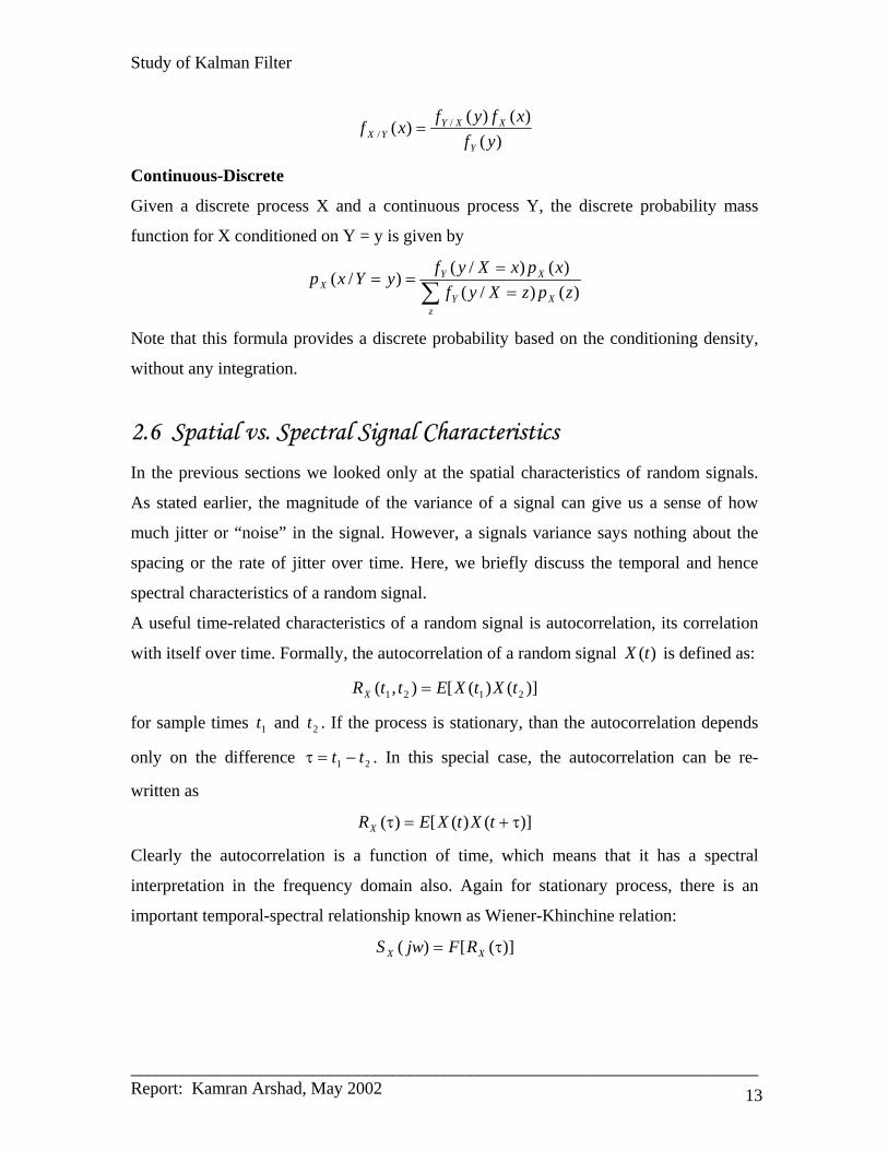
Note that this formula provides a discrete probability based on the conditioning density,

without any integration.

2.6 Spatial vs. Spectral Signal Characteristics In the previous sections we looked only at the spatial characteristics of random signals.

As stated earlier, the magnitude of the variance of a signal can give us a sense of how

much jitter or “noise” in the signal. However, a signals variance says nothing about the

spacing or the rate of jitter over time. Here, we briefly discuss the temporal and hence

spectral characteristics of a random signal.

A useful time-related characteristics of a random signal is autocorrelation, its correlation

with itself over time. Formally, the autocorrelation of a random signal )(tX is defined as:

)]()([),( 2121 tXtXEttRX =

for sample times 1t and 2t . If the process is stationary, than the autocorrelation depends

only on the difference 21 tt −=τ . In this special case, the autocorrelation can be re-

written as

)]()([)( τ+=τ tXtXERX

Clearly the autocorrelation is a function of time, which means that it has a spectral

interpretation in the frequency domain also. Again for stationary process, there is an

important temporal-spectral relationship known as Wiener-Khinchine relation:

)]([)( τ= XX RFjwS



Chapter 3

Discrete Kalman Filter In 1960, R.E. Kalman published his famous paper describing a recursive solution to the

discrete-data linear filtering problem [Kalman60]. Since that time, due in large part to

advances in digital computing, the Kalman filter has been the subject of extensive

research and application, particularly in the area of autonomous or assisted navigation. A

very "friendly" introduction to the general idea of the Kalman filter can be found in

Chapter 1 of [Maybeck79], while a more complete introductory discussion can be found

in [Sorenson70], which also contains some interesting historical narrative. More

extensive references include [Gelb74; Grewal93; Maybeck79; Lewis86; Brown92;

Jacobs93].

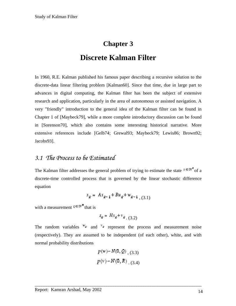
3.1 The Process to be Estimated

The Kalman filter addresses the general problem of trying to estimate the state of a

discrete-time controlled process that is governed by the linear stochastic difference

equation

, (3.1)

with a measurement that is

. (3.2)

The random variables and represent the process and measurement noise

(respectively). They are assumed to be independent (of each other), white, and with

normal probability distributions

, (3.3)

. (3.4)



In practice, the process noise covariance and measurement noise covariance matrices

might change with each time step or measurement, however here we assume they are

constant.

The matrix in the difference equation (3.1) relates the state at the previous time

step to the state at the current step , in the absence of either a driving function or

process noise. Note that in practice might change with each time step, but here we

assume it is constant. The matrix B relates the optional control input to the

state x. The matrix in the measurement equation (3.2) relates the state to the

measurement Zk. In practice might change with each time step or measurement, but

here we assume it is constant.

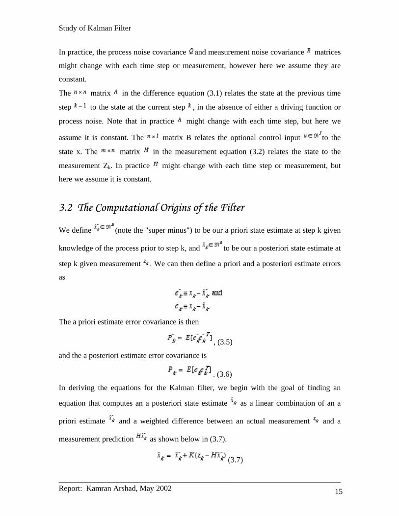
3.2 The Computational Origins of the Filter

We define (note the "super minus") to be our a priori state estimate at step k given

knowledge of the process prior to step k, and to be our a posteriori state estimate at

step k given measurement . We can then define a priori and a posteriori estimate errors

as

The a priori estimate error covariance is then

, (3.5)

and the a posteriori estimate error covariance is

. (3.6)

In deriving the equations for the Kalman filter, we begin with the goal of finding an

equation that computes an a posteriori state estimate as a linear combination of an a

priori estimate and a weighted difference between an actual measurement and a

measurement prediction as shown below in (3.7).

(3.7)



The difference in (3.7) is called the measurement innovation, or the residual.

The residual reflects the discrepancy between the predicted measurement and the

actual measurement . A residual of zero means that the two are in complete agreement.

The matrix K in (3.7) is chosen to be the gain or blending factor that minimizes the

a posteriori error covariance (3.6). This minimization can be accomplished by first

substituting (3.7) into the above definition for , substituting that into (3.6), performing

the indicated expectations, taking the derivative of the trace of the result with respect to

K, setting that result equal to zero, and then solving for K. For more details see

[Maybeck79; Brown92; Jacobs93]. One form of the resulting K that minimizes (3.6) is

given by

. (3.8)

Looking at (3.8) we see that as the measurement error covariance approaches zero, the

gain K weights the residual more heavily. Specifically,

On the other hand, as the a priori estimate error covariance approaches zero, the gain

K weights the residual less heavily. Specifically,

Another way of thinking about the weighting by K is that as the measurement error

covariance approaches zero, the actual measurement is "trusted" more and more,

while the predicted measurement is trusted less and less. On the other hand, as the a

priori estimate error covariance approaches zero the actual measurement is trusted

less and less, while the predicted measurement is trusted more and more.



3.3 The Probabilistic Origins of the Filter

The justification for (3.7) is rooted in the probability of the a priori estimate

conditioned on all prior measurements (Bayes' rule). For now let it suffice to point out

that the Kalman filter maintains the first two moments of the state distribution,

The a posteriori state estimate (3.7) reflects the mean (the first moment) of the state

distribution-- it is normally distributed if the conditions of (3.3) and (3.4) are met. The a

posteriori estimate error covariance (3.6) reflects the variance of the state distribution (the

second non-central moment). In other words,

.

For more details on the probabilistic origins of the Kalman filter, see [Maybeck79;

Brown92; Jacobs93].

3.4 The Discrete Kalman Filter Algorithm We will begin this section with a broad overview, covering the "high-level" operation of

one form of the discrete Kalman filter (see the previous footnote). After presenting this

high-level view, we will narrow the focus to the specific equations and their use in this

version of the filter.

The Kalman filter estimates a process by using a form of feedback control: the filter

estimates the process state at some time and then obtains feedback in the form of (noisy)

measurements. As such, the equations for the Kalman filter fall into two groups: time

update equations and measurement update equations. The time update equations are

responsible for projecting forward (in time) the current state and error covariance

estimates to obtain the a priori estimates for the next time step. The measurement update

equations are responsible for the feedback--i.e. for incorporating a new measurement into

the a priori estimate to obtain an improved a posteriori estimate.



The time update equations can also be thought of as predictor equations, while the

measurement update equations can be thought of as corrector equations. Indeed the final

estimation algorithm resembles that of a predictor-corrector algorithm for solving

numerical problems as shown below in Figure 3-1.

Time

Update Measurement

(Predict) Update (correct)

Figure 3-1. The ongoing discrete Kalman filter cycle. The time update projects the

current state estimate ahead in time. The measurement update adjusts the projected

estimate by an actual measurement at that time.

The specific equations for the time and measurement updates are presented below in

Table 3-1 and Table 3-2.

Table 3-1: Discrete Kalman filter time update equations.

(3.9)

(3.10)

Again notice how the time update equations in Table 3-1 project the state and covariance

estimates forward from time step to step . A and B are from (3.1), while is from

(3.3). Initial conditions for the filter are discussed in the earlier references.



Table 3-2: Discrete Kalman filter measurement update equations.

(3.11)

(3.12)

(3.13)

The first task during the measurement update is to compute the Kalman gain, . Notice

that the equation given here as (3.11) is the same as (3.8). The next step is to actually

measure the process to obtain , and then to generate an a posteriori state estimate by

incorporating the measurement as in (3.12). Again (3.12) is simply (3.7) repeated here for

completeness. The final step is to obtain an a posteriori error covariance estimate via

(3.13).

After each time and measurement update pair, the process is repeated with the previous a

posteriori estimates used to project or predict the new a priori estimates. This recursive

nature is one of the very appealing features of the Kalman filter--it makes practical

implementations much more feasible than (for example) an implementation of a Wiener

filter [Brown92] which is designed to operate on all of the data directly for each estimate.

The Kalman filter instead recursively conditions the current estimate on all of the past

measurements.Figure 3-2 below offers a complete picture of the operation of the filter,

combining the high-level diagram of Figure 3-1 with the equations from Table 3-1 and

Table 3-2.

3.5 Filter Parameters and Tuning

In the actual implementation of the filter, the measurement noise covariance is usually

measured prior to operation of the filter. Measuring the measurement error covariance

is generally practical (possible) because we need to be able to measure the process

anyway (while operating the filter) so we should generally be able to take some off-line

sample measurements in order to determine the variance of the measurement noise.



The determination of the process noise covariance is generally more difficult as we

typically do not have the ability to directly observe the process we are estimating.

Sometimes a relatively simple (poor) process model can produce acceptable results if one

"injects" enough uncertainty into the process via the selection of . Certainly in this case

one would hope that the process measurements are reliable.

In either case, whether or not we have a rational basis for choosing the parameters, often

times superior filter performance (statistically speaking) can be obtained by tuning the

filter parameters and . The tuning is usually performed off-line, frequently with the

help of another (distinct) Kalman filter in a process generally referred to as system

identification.

Figure 3-2. A complete picture of the operation of the Kalman filter, combining the high-

level diagram of Figure 3-1 with the equations from Table 3-1 and Table 3-2

In closing we note that under conditions where and are in fact constant, both the

estimation error covariance and the Kalman gain will stabilize quickly and then

remain constant (see the filter update equations in Figure 3-2). If this is the case, these

parameters can be pre-computed by either running the filter off-line, or for example by

determining the steady-state value of as described in [Grewal93].

It is frequently the case however that the measurement error (in particular) does not

remain constant. For example, when sighting beacons in our optoelectronic tracker



ceiling panels, the noise in measurements of nearby beacons will be smaller than that in

far-away beacons. Also, the process noise is sometimes changed dynamically during

filter operation becoming in order to adjust to different dynamics. For example, in the

case of tracking the head of a user of a 3D virtual environment we might reduce the

magnitude of if the user seems to be moving slowly, and increase the magnitude if the

dynamics start changing rapidly. In such cases might be chosen to account for both

uncertainty about the user's intentions and uncertainty in the model.



Chapter 4

Extended Kalman Filter

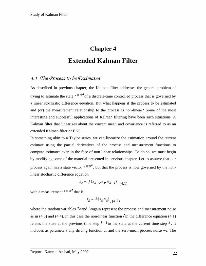
4.1 The Process to be Estimated As described in previous chapter, the Kalman filter addresses the general problem of

trying to estimate the state of a discrete-time controlled process that is governed by

a linear stochastic difference equation. But what happens if the process to be estimated

and (or) the measurement relationship to the process is non-linear? Some of the most

interesting and successful applications of Kalman filtering have been such situations. A

Kalman filter that linearizes about the current mean and covariance is referred to as an

extended Kalman filter or EKF.

In something akin to a Taylor series, we can linearize the estimation around the current

estimate using the partial derivatives of the process and measurement functions to

compute estimates even in the face of non-linear relationships. To do so, we must begin

by modifying some of the material presented in previous chapter. Let us assume that our

process again has a state vector , but that the process is now governed by the non-

linear stochastic difference equation

, (4.1)

with a measurement that is

, (4.2)

where the random variables and again represent the process and measurement noise

as in (4.3) and (4.4). In this case the non-linear function in the difference equation (4.1)

relates the state at the previous time step to the state at the current time step . It

includes as parameters any driving function uk and the zero-mean process noise wk. The



non-linear function in the measurement equation (4.2) relates the state to the

measurement .

In practice of course one does not know the individual values of the noise and at

each time step. However, one can approximate the state and measurement vector without

them as

(4.3)

and

, (4.4)

where is some a posteriori estimate of the state (from a previous time step k).

It is important to note that a fundamental flaw of the EKF is that the distributions (or

densities in the continuous case) of the various random variables are no longer normal

after undergoing their respective nonlinear transformations. The EKF is simply an ad hoc

state estimator that only approximates the optimality of Bayes' rule by linearization.

Some interesting work has been done by Julier et al. in developing a variation to the EKF,

using methods that preserve the normal distributions throughout the non-linear

transformations [Julier96].

4.2 The Computational Origins of the Filter To estimate a process with non-linear difference and measurement relationships, we

begin by writing new governing equations that linearize an estimate about (4.3) and (4.4),

, (4.5)

. (4.6)

where

and are the actual state and measurement vectors,

and are the approximate state and measurement vectors from (4.3) and (4.4),

is an a posteriori estimate of the state at step k,

the random variables and represent the process and measurement noise as in (4.3)

and (4.4).



A is the Jacobian matrix of partial derivatives of with respect to x, that is

,

W is the Jacobian matrix of partial derivatives of with respect to w,

,

H is the Jacobian matrix of partial derivatives of with respect to x,

,

V is the Jacobian matrix of partial derivatives of with respect to v,

.

Note that for simplicity in the notation we do not use the time step subscript with the

Jacobians , , , and , even though they are in fact different at each time step.

Now we define a new notation for the prediction error,

, (4.7)

and the measurement residual,

. (4.8)

Remember that in practice one does not have access to in (4.7), it is the actual state

vector, i.e. the quantity one is trying to estimate. On the other hand, one does have access

to in (4.8), it is the actual measurement that one is using to estimate . Using (4.7) and

(4.8) we can write governing equations for an error process as

, (4.9)

, (4.10)

where and represent new independent random variables having zero mean and

covariance matrices and , with and as in (4.3) and (4.4) respectively.

Notice that the equations (4.9) and (4.10) are linear, and that they closely resemble the

difference and measurement equations (4.1) and (4.2) from the discrete Kalman filter.



This motivates us to use the actual measurement residual in (4.8) and a second

(hypothetical) Kalman filter to estimate the prediction error given by (4.9). This

estimate, call it , could then be used along with (4.7) to obtain the a posteriori state

estimates for the original non-linear process as

. (4.11)

The random variables of (4.9) and (4.10) have approximately the following probability

distributions (see the previous footnote):

Given these approximations and letting the predicted value of be zero, the Kalman

filter equation used to estimate is

. (4.12)

By substituting (4.12) back into (4.11) and making use of (4.8) we see that we do not

actually need the second (hypothetical) Kalman filter:

(4.13)

Equation (4.13) can now be used for the measurement update in the extended Kalman

filter, with and coming from (4.3) and (4.4), and the Kalman gain coming from

(4.11) with the appropriate substitution for the measurement error covariance.

The complete set of EKF equations is shown below in Table 4-1 and Table 4-2. Note that

we have substituted for to remain consistent with the earlier "super minus" a priori

notation, and that we now attach the subscript to the Jacobians , , , and , to

reinforce the notion that they are different at (and therefore must be recomputed at) each

time step.



Table 4-1: EKF time update equations.

(4.14)

(4.15)

As with the basic discrete Kalman filter, the time update equations in Table 4-1 project

the state and covariance estimates from the previous time step to the current time

step . Again in (4.14) comes from (4.3), and are the process Jacobians at step k,

and is the process noise covariance (4.3) at step k.

Table 4-2: EKF measurement update equations.

(4.16)

(4.17)

(4.18)

As with the basic discrete Kalman filter, the measurement update equations in Table 4-2

correct the state and covariance estimates with the measurement . Again in (4.17)

comes from (4.4), and V are the measurement Jacobians at step k, and is the

measurement noise covariance (4.4) at step k. (Note we now subscript allowing it to

change with each measurement).

The basic operation of the EKF is the same as the linear discrete Kalman filter as shown

in Figure 4-1. Figure 4-1 below offers a complete picture of the operation of the EKF,


Table 4-2.



Figure 4-1. A complete picture of the operation of the extended Kalman filter,


Table 4-2.

An important feature of the EKF is that the Jacobian in the equation for the Kalman

gain serves to correctly propagate or "magnify" only the relevant component of the

measurement information. For example, if there is not a one-to-one mapping between the

measurement and the state via , the Jacobian affects the Kalman gain so that it

only magnifies the portion of the residual that does affect the state. Of course if

over all measurements there is not a one-to-one mapping between the measurement

and the state via , then as you might expect the filter will quickly diverge. In this case

the process is unobservable.

4.3 Applications The EKF has been applied extensively to the field of nonlinear estimation. General

application areas may be divided into state-estimation and machine learning. We further

divide machine learning into parameter estimation and dual estimation. The framework

for these areas are briefly reviewed next.



4.3.1 State Estimation

The basic framework for the EKF involves estimation of the state of a discrete-time

nonlinear dynamic system,

(1)

(2)

where represent the unobserved state of the system and is the only observed

signal. The process noise drives the dynamic system, and the observation noise is

given by . Note that we are not assuming additivity of the noise sources. The system

dynamic model and are assumed known.

In state-estimation, the EKF is the standard method of choice to achieve a recursive

(approximate) maximum-likelihood estimation of the state .

4.3.2 Parameter Estimation

The classic machine learning problem involves determining a nonlinear mapping

(3)

where is the input, is the output, and the nonlinear map is parameterized by the

vector . The nonlinear map, for example, may be a feedforward or recurrent neural

network ( are the weights), with numerous applications in regression, classification,

and dynamic modeling. Learning corresponds to estimating the parameters . Typically,

a training set is provided with sample pairs consisting of known input and desired

outputs, . The error of the machine is defined as , and the

goal of learning involves solving for the parameters in order to minimize the expected

squared error.



While a number of optimization approaches exist (e.g., gradient descent using

backpropagation), the EKF may be used to estimate the parameters by writing a new

state-space representation

(4)

(5)

where the parameters correspond to a stationary process with identity state transition

matrix, driven by process noise (the choice of variance determines tracking

performance). The output corresponds to a nonlinear observation on . The EKF

can then be applied directly as an efficient ``second-order'' technique for learning the

parameters. In the linear case, the relationship between the Kalman Filter (KF) and

Recursive Least Squares (RLS) is given in [2]. The use of the EKF for training neural

networks has been developed by Singhal and Wu [3] and Puskorious and Feldkamp [4].

4.3.3 Dual Estimation

A special case of machine learning arises when the input is unobserved, and requires

coupling both state-estimation and parameter estimation. For these dual estimation

problems, we again consider a discrete-time nonlinear dynamic system,

(6)

(7)

where both the system states and the set of model parameters for the dynamic

system must be simultaneously estimated from only the observed noisy signal .

In the next section we explain the basic assumptions and flaws with the using the EKF. In

Section 6.1, we introduce the Unscented Kalman Filter (UKF) as a method to amend the

flaws in the EKF.



4.4 Basic Flaw In EKF Consider the basic state-space estimation framework as in Equations 1 and 2. Given the

noisy observation , a recursive estimation for can be expressed in the form (see

[5]),

(8)

This recursion provides the optimal minimum mean-squared error (MMSE) estimate for

assuming the prior estimate and current observation are Gaussian Random

Variables (GRV). We need not assume linearity of the model. The optimal terms in this

recursion are given by

(9)

(10)

(11)

where the optimal prediction of is written as , and corresponds to the expectation

of a nonlinear function of the random variables and (similar interpretation for

the optimal prediction ). The optimal gain term is expressed as a function of

posterior covariance matrices (with ). Note these terms also require taking

expectations of a nonlinear function of the prior state estimates.

The Kalman filter calculates these quantities exactly in the linear case, and can be viewed

as an efficient method for analytically propagating a GRV through linear system

dynamics. For nonlinear models, however, the EKF approximates the optimal terms as:



(12)

(13)

(14)

where predictions are approximated as simply the function of the prior mean value for

estimates (no expectation taken) The covariance are determined by linearizing the

dynamic equations , and then determining the

posterior covariance matrices analytically for the linear system. In other words, in the

EKF the state distribution is approximated by a GRV which is then propagated

analytically through the ``first-order'' linearization of the nonlinear system. The readers

are referred to [5] for the explicit equations. As such, the EKF can be viewed as

providing ``first-order'' approximations to the optimal terms. These approximations,

however, can introduce large errors in the true posterior mean and covariance of the

transformed (Gaussian) random variable, which may lead to sub-optimal performance

and sometimes divergence of the filter. It is these ``flaws'' which will be amended in the

next section using the UKF.



Chapter 5

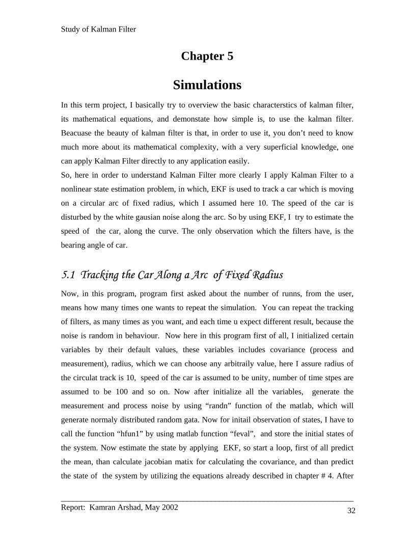
Simulations In this term project, I basically try to overview the basic characterstics of kalman filter,

its mathematical equations, and demonstate how simple is, to use the kalman filter.

Beacuase the beauty of kalman filter is that, in order to use it, you don’t need to know

much more about its mathematical complexity, with a very superficial knowledge, one

can apply Kalman Filter directly to any application easily.

So, here in order to understand Kalman Filter more clearly I apply Kalman Filter to a

nonlinear state estimation problem, in which, EKF is used to track a car which is moving

on a circular arc of fixed radius, which I assumed here 10. The speed of the car is

disturbed by the white gausian noise along the arc. So by using EKF, I try to estimate the

speed of the car, along the curve. The only observation which the filters have, is the

bearing angle of car.

5.1 Tracking the Car Along a Arc of Fixed Radius Now, in this program, program first asked about the number of runns, from the user,

means how many times one wants to repeat the simulation. You can repeat the tracking

of filters, as many times as you want, and each time u expect different result, because the

noise is random in behaviour. Now here in this program first of all, I initialized certain

variables by their default values, these variables includes covariance (process and

measurement), radius, which we can choose any arbitraily value, here I assure radius of

the circulat track is 10, speed of the car is assumed to be unity, number of time stpes are

assumed to be 100 and so on. Now after initialize all the variables, generate the

measurement and process noise by using “randn” function of the matlab, which will

generate normaly distributed random gata. Now for initail observation of states, I have to

call the function “hfun1” by using matlab function “feval”, and store the initial states of

the system. Now estimate the state by applying EKF, so start a loop, first of all predict

the mean, than calculate jacobian matix for calculating the covariance, and than predict

the state of the system by utilizing the equations already described in chapter # 4. After



calculating all the estimated values, than calculating the error, simply by taking the

difference between the actual value and the predicted value of state. Now than taking its

square root, and calculating the mean square error of prediction. Ideally this error should

be zero. Finally I will display all the results as shown below.



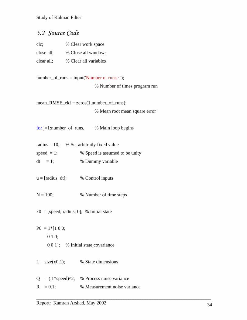
5.2 Source Code clc; % Clear work space

close all; % Close all windows

clear all; % Clear all variables

number_of_runs = input('Number of runs : ');

% Number of times program run

mean_RMSE_ekf = zeros(1,number_of_runs);

% Mean root mean square error

for j=1:number_of_runs, % Main loop begins

radius = 10; % Set arbitraily fixed value

speed = 1; % Speed is assumed to be unity

dt = 1; % Dummy variable

u = [radius; dt]; % Control inputs

N = 100; % Number of time steps

x0 = [speed; radius; 0]; % Initial state

P0 = 1*[1 0 0;

0 1 0;

0 0 1]; % Initial state covariance

L = size(x0,1); % State dimensions

Q = (.1*speed)^2; % Process noise variance

R = 0.1; % Measurement noise variance



xh = zeros(L,N+1); % State estimate buffer

P = zeros(L,L,1,N+1);% State covariance buffer

xh(:,1) = x0; % initialize buffers

Px(:,:,1) = P0;

xh_ekf = xh; % Create EKF buffers from template

P_ekf = Px;

alpha = 1;

beta = 2;

kappa = 0; % 3 - state dimension

%%-------------------------------------------------------------------

%%---------------------- GENERATE DATASET ---------------------------

fprintf('\nGenerating data...\n');

x = zeros(L,N+1);

y = zeros(1,N+1);

v = sqrt(Q)*randn(1,N+1); % Process noise

n = sqrt(R)*randn(1,N+1); % Measurement noise

x(:,1) = x0; % Initial state condition

y(:,1) = feval('hfun1',x(:,1),u,n(:,1),1);

% Initial onbservation of state

for k=2:(N+1),

x(:,k) = feval('ffun1',x(:,k-1),u,v(:,k),k);



y(:,k) = feval('hfun1',x(:,k),u,n(:,k),k);

end

%%-------------------------------------------------------------------

%%------------------- ESTIMATE STATE USING EKF ----------------------

fprintf('\nEstimating trajectory...\n');

for k=2:(N+1),

% Generate EKF estimate

xPred_ekf = feval('ffun1',xh_ekf(:,k-1),u,0,k);

% EKF predicted mean

Jx = jacobian_ffun1(xh_ekf(:,k-1),u);

% Jacobian for ffun1

PPred_ekf = diag([Q 0 0]) + Jx*P_ekf(:,:,k-1)*Jx';

% EKF predicted state covariance

yPred = feval('hfun1',xPred_ekf,u,0,k);

Jy = jacobian_hfun1(xPred_ekf,u); % Jacobian for hfun1

% Calculations

S = R + Jy*PPred_ekf*Jy';

Si = inv(S);

K = PPred_ekf*Jy'*Si;

xh_ekf(:,k) = xPred_ekf + K*(y(:,k)-yPred);

% Predicted state estimate

P_ekf(:,:,k) = PPred_ekf - K*Jy*PPred_ekf;

end

%%-------------------------------------------------------------------



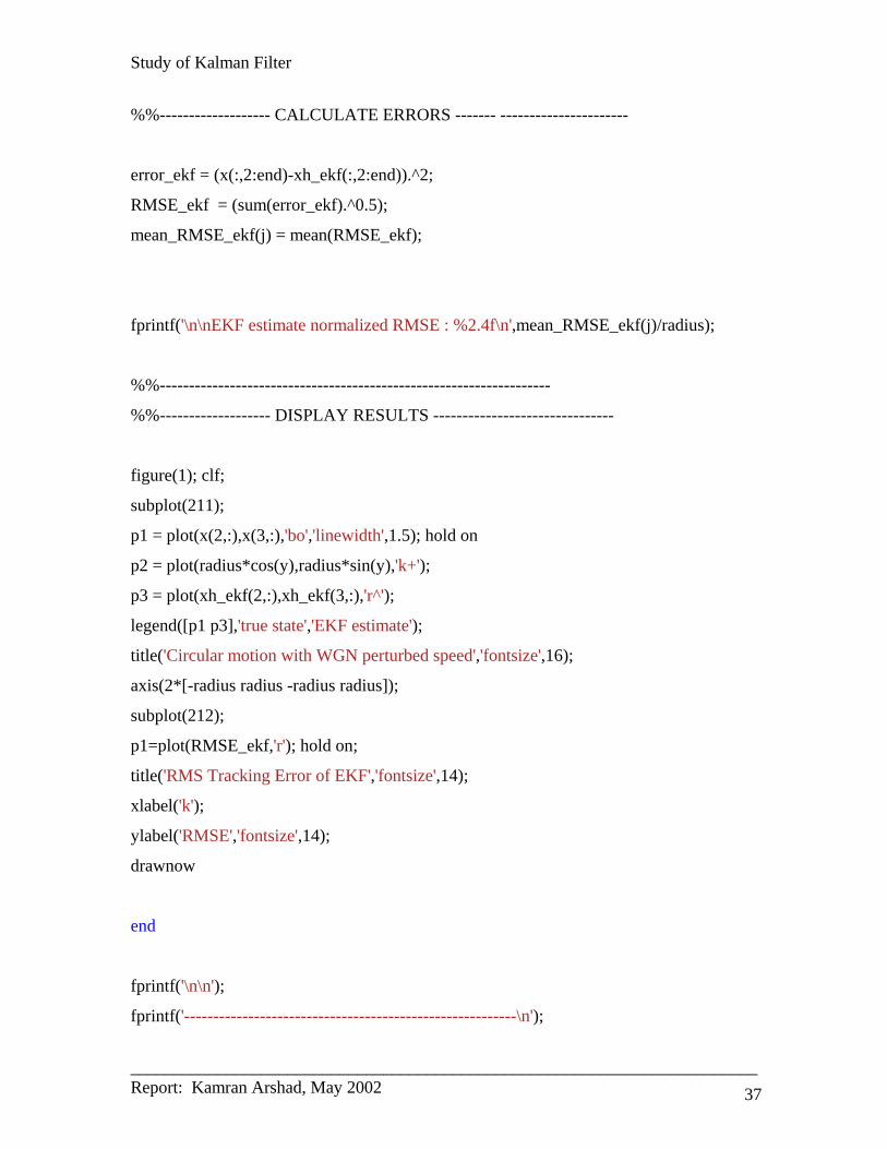
%%------------------- CALCULATE ERRORS ------- ----------------------

error_ekf = (x(:,2:end)-xh_ekf(:,2:end)).^2;

RMSE_ekf = (sum(error_ekf).^0.5);

mean_RMSE_ekf(j) = mean(RMSE_ekf);

fprintf('\n\nEKF estimate normalized RMSE : %2.4f\n',mean_RMSE_ekf(j)/radius);

%%-------------------------------------------------------------------

%%------------------- DISPLAY RESULTS -------------------------------

figure(1); clf;

subplot(211);

p1 = plot(x(2,:),x(3,:),'bo','linewidth',1.5); hold on

p2 = plot(radius*cos(y),radius*sin(y),'k+');

p3 = plot(xh_ekf(2,:),xh_ekf(3,:),'r^');

legend([p1 p3],'true state','EKF estimate');

title('Circular motion with WGN perturbed speed','fontsize',16);

axis(2*[-radius radius -radius radius]);

subplot(212);

p1=plot(RMSE_ekf,'r'); hold on;

title('RMS Tracking Error of EKF','fontsize',14);

xlabel('k');

ylabel('RMSE','fontsize',14);

drawnow

end

fprintf('\n\n');

fprintf('---------------------------------------------------------\n');



fprintf('Mean & Variance of normalized RMSE over %d runs\n\n',number_of_runs);

fprintf('EKF : %2.4f

(%2.4f)\n',mean(mean_RMSE_ekf/radius),var(mean_RMSE_ekf/radius));

fprintf('---------------------------------------------------------\n');

5.3 Simulation Results Now when we run the above program, only once, and try to estimate the speed of the car

which is moving on a circular arc of radius 10, we have following results, how the EKF

track the actual state, as well as I also plot here the mean square error for the reference,

because it shows clrealy how much the EKF succeded in estimating the state.

-20 -15 -10 -5 0 5 10 15 20-20

-10

0

10

20Circular motion with WGN perturbed speed

true stateEKF estimate

0 10 20 30 40 50 60 70 80 90 1000

5

10

15

20RMS Tracking Error of EKF

k

RM

SE

Similarly, for many runs, the screen will show you the trajectory traced by the EKF in

each run. The filter, basically calculate the bearing angle in each case, and than based on

that angle, they will estimate the current states, by using relations already described

earlier.



So for many runs,

-20 0 20-20

-10

0

10

20cular motion with AWGN perturbed speed

true stateEKF estimate

-20 0 20-20

-10

0

10

20

-20 0 20-20

-10

0

10

20

-20 0 20-20

-10

0

10

20

-20 0 20-20

-10

0

10

20

-20 0 20-20

-10

0

10

20

Similarlay, we can plot the RMS tracking error, in each case, as we already know, lower

the tracking error better will be the performance. So, the RMS tracking error is given as,



0 50 1000

10

20

30RMS Tracking Error of EKF

k

RM

SE

0 50 1000

5

10

15

20

25

k

RM

SE

0 50 1000

10

20

30

k

RM

SE

0 50 1000

1

2

3

k

RM

SE

0 50 1000

5

10

15

20

25

k

RM

SE

0 50 1000

5

10

15

20

kR

MS

E

So, its quite clear from the above curves of mean square error, that sometimes the mean

square error is high and sometimes its settles to a moderate level.

5.2 Conclusion Here in this term project, I review the basic concepts of estimation in the light of Kalman

Filter. Kalman Filter is basically a set of mathematical equations which are used for the

estimation of states. For nonlinear state estimation problems, we use extended kalman

filter, which is a very powerful mathematical tool. After studing the basics of kalman

filters, I than apply kalman filter on a nonlinear state estimation problem. Form the above

simulation results, its quite clear that extended kalman filter can be successfully used for

the nonlinear state estimation problem, since the process is random, so in each itteration

we have different mean square error, but in general, the level of mean square error, is

within permissible limits, so EKF can be used without any doubt to nonlinea estimation

problem. Anyone can also extend my work, so there is also a suggestion for those who

have interest in this area, and wants to extend my work. There is another modification of



EKF so called UKF (Uncented Kalman Filter) whose performance is better than EKF, so

anybody can extend this work by applying UKF on the same problem, and than compare

the results of the two filters.



REFRENCES

[1] S. J. Julier and J. K. Uhlmann.

A New Extension of the Kalman Filter to Nonlinear Systems. In Proc. of AeroSense: The 11th Int. Symp. on Aerospace/Defence Sensing, Simulation and Controls., 1997.

[2] Simon Haykin. Adaptive Filter Theory. Prentice-Hall, Inc, 3 edition, 1996.

[3] S. Singhal and L. Wu. Training multilayer perceptrons with the extended Kalman filter. In Advances in Neural Information Processing Systems 1, pages 133-140, San Mateo, CA, 1989. Morgan Kauffman.

[4] G.V. Puskorius and L.A. Feldkamp. Decoupled Extended Kalman Filter Training of Feedforward Layered Networks. In IJCNN, volume 1, pages 771-777, 1991.

[5] Frank L. Lewis. Optimal Estimation. John Wiley & Sons, Inc., New York, 1986.

[6] Simon J. Julier. The Scaled Unscented Transformation. To appear in Automatica, February 2000

king fahd university of petroleum & mineralsfaculty.kfupm.edu.sa/ee/akamran/ee550.pdf · king...

Documents