1

Kinetics of Reaction Systems

Sheryl Hemkin Department of Chemistry

Kenyon College Gambier, Ohio 43050

hemkins@kenyon.edu

~ Aims of Module ~

The module was designed to give students an understanding of the kinetics associated with reaction systems (small groups of reactions that are chemically tied together). To that end, the module will also introduce the students to a low cost molecular visualization program, Berkeley Madonna. (You are also able to download a demo copy.) By learning how to translate rate equations into the coding structure of Berkeley Madonna the students will be able to independently simulate how the reactions’ chemical concentrations will change with time.

~ Minimum Student Background ~

Chemistry/biochemistry: general chemistry with a brief into kinetics (details below) Molecular Visualization: no experience required The background sections of this module will refresh the students’ memory about how to construct rate equations, particularly with respect to systems of chemical reactions, as well as introduce the ideas behind numerical simulations of rate laws (which are ordinary differential equations, ODEs). With respect to the kinetics, it is most ideal that the students have had a basic lecture or two on rate laws before attempting this module. Some familiarity with basic biology and differential equations and integration is helpful, but not required. As this module was created to enhance the understanding of kinetics via simulation and how simulation can be used in advancing kinetic/mechanistic research, the problem sets at the end of each section reflect a range of difficulties. Thus the instructor should examine the questions ahead of time to determine which suit the purpose of the target audience.

~ Keywords ~

simulation, rate laws, steady state, oscillation, enzyme kinetics

2

Kinetics of Reaction Systems

To look closely at the world around you is to see that the environment is composed of many intricately entwined chemical reactions, such as the degradation of ozone in the atmosphere, the production of melatonin in the body, and the decomposition of leaves in the forest. While extremely important to the maintenance of life and the environment, these reaction systems are rarely thought of in terms of the underlying chemical reactions that drive them and govern their behavior. Historically, the lack of investigation was due to the complexities that characterize these reactions. However, due to technological improvements researchers are now able to push these boundaries both in the areas of experiment and simulation. In general, the simulations are carried out using a representative set of rate equations developed using information gained from experiment and theory. However these investigations become especially useful when there is a dearth of knowledge, as simulation allows for the testing and examination of hypotheses that are not easily substantiated by experiment. This module was developed for two purposes, to give students a basic understanding of this type of numerical simulation and to further their understanding of kinetics (in particular how rate constants and initial concentrations affect outcome) using both equilibrium and far from equilibrium chemical examples. Most of the kinetics learned and examined in chemistry lecture and lab consist of examining chemical reactions that naturally goes to a constant concentration, at which point the forward rate is equal to the reverse rate. These examples generally involve a single elementary reaction where the reactants go to a lower concentration and the products go to a higher concentration, for example in the dimerization of NO2.

3

As you will see, the behavior (how concentrations change over time) of these single-step elementary reactions is relatively easy to predict and understand after formulating the rate law, and rate laws are relatively easy to construct for such reactions. Unfortunately most chemical reactions are not so easy to characterize. As can be imagined, not all chemistry of interest results from one individual elementary chemical reaction working alone. Often a scientific question or concern involves a reaction system, a multitude of elementary reactions working in concert, such as in the production of melatonin in the human body. While these reaction systems are certainly very interesting, in the majority of cases they are not well characterized in terms of the constituent elementary reactions; therefore, the rate equations must be created from a combination of experiment, theory and occasionally, chemical intuition. In this exercise, you will not only have the opportunity to create rate equations for reaction systems with known or postulated mechanisms, but you will also be given a brief introduction to the creation and development of rate equations for a reaction with an unknown mechanism. In all cases, you will be able to use simulation to help understand how rate constants and initial conditions can affect the behavior of the system. Finally, in the last section you will work with a model that has the ability to generate a range of outcomes from steady state to periodic and chaotic oscillations. To accomplish all this, a basic working knowledge of the field of kinetics is required. In the broad sense, kinetics is the study of the speed or rate at which a process (like driving or a chemical reaction) proceeds. Typically when thinking about rate, it takes on the description of the past or the present, for example, “they were eating 10 hotdogs per minute until they got sick” or “the reactant concentration is decreasing at a rate of 0.1 moles per liter per minute.” Nevertheless, one of the most powerful and enlightening ways to use kinetics is to envision and predict the future. Consequently, an understanding of the rate equations that underlie a process will allow us to make general forecasts and/or more specific predictions, i.e. to generally speculate if a chemical’s concentration will increase or decrease during reaction, or to more specifically predict if a product’s concentration will increase steadily over the course of an hour or if it will rise quickly in the first minute then gently increase. But before this is possible, it is imperative to have an understanding of rate equations and how they are constructed.

4

CONTENTS

Building Rate Laws.

Rate Laws, ODEs and Integration.

Numerical Methods and Simulation.

Steady State and Oscillatory Behavior.

Important notes for the use of Berkeley Madonna.

Section 1 Equilibrium

Section 2 Enzyme Kinetics

Section 3 Simulations and Mechanisms

Section 4 Oscillations

5

Building Rate Laws (Rate Laws also known as Rate Equations)

To quickly review the concepts, it should first be known that the rate at which a reaction proceeds is proportional to the reactant concentration(s) raised to a power called the order. Since a proportionality is not so straightforward to work with, the rate constant is introduced to create an equality between the rate and concentrations. For example,

!

example 1. a A + b B " d D

rate # [A]X

[B]Y

(proportionality) rate = k [A]X

[B]Y

(equality)

where k is the rate constant, X is the order with respect to A, and Y is the order with respect to B.

The value of the order can be found a variety of ways depending on the circumstances. If the reaction equation is elementary, i.e. a reaction that cannot be broken down into a smaller step, the value of the order is equal to the reactant’s stoichiometric coefficient. (If the example above illustrated an elementary reaction, rate = k [A]a [B]b.) Often though, knowledge of the reaction is not detailed enough to write elementary reactions; in these cases, the values for the orders must be determined experimentally. Similarly the value of the rate constant is found by experiment. (An introductory chemistry book should outline some potential experimental scenarios that would yield the values of the orders and rate constants.) Finally, to complete the rate law, “rate” must be described mathematically. To utilize these rate laws properly, a clarification of the word “rate” is needed. As this word is often used in multiple senses, such as to refer to the rate of reaction, or the rate of change in the concentration of a chemical, it is important to recognize what form of “rate” is being used. In general, for reaction kinetics, the rate is defined as the change in the concentration of chemical X within a specific amount of time, Δ[chemical X]/Δt. For most purposes however, the specified time period will be an instant, which allows this rate to be defined with the following notation from calculus, d[chemical X]/dt. The rate of reaction is an extension of this general idea, with modifications made to account for the global aspects of the reaction. Using example 1,

!

rate of reaction (ex. 1) = k [A]X

[B]Y

with the definition :

rate of reaction (ex. 1) = " 1

a

d[A]

dt = "

1

b

d[B]

dt = +

1

d

d[D]

dt (eq. 1)

As can be seen in equation 1, the rate of reaction can be characterized in multiple ways, with the root of each corresponding to a reactant or product of the reaction. Also, as indicated by the equal signs, each of these definitions must have the same numerical value, the value that indicates the rate of the reaction’s progress at a given moment. In order to achieve this equality, a positive sign is added to the rate of concentration change if the chemical involved is a product, as the product concentration increases during the reaction. In contrast, the rate definition will have a negative

6

sign if the chemical is a reactant, as this concentration will decrease over time. Furthermore, the rate of concentration change will be multiplied by the inverse of the respective stoichiometric coefficient (ex. 1/a). These modifications allow the unification of the definitions; thus, despite example 1 having three different ways to characterize the rate of reaction, each of those definitions will have the same numerical value. This value relays information about the progress of the reaction as a whole and is more formally referred to as the ‘rate of change of the extent of the reaction.’ For the reaction simulations done in this exercise, the input required will be the rate of concentration change; that is, knowledge of d[chemical X]/dt is required. This means the positive/negative signs and the inverted stoichiometric constants discussed in the previous paragraph will be algebraically moved to the rate constant side of the reaction. For example 1, a one step reaction, the needed rate expressions for simulation would be as follows,

!

d[ A]

dt O = " a k[ A]

X[ B]

Y

d [ B]

dt = " b k[ A]

X[ B]

Y

d [ D]

dt = + d k[ A]

X[ B]

Y (eq. 2)

Of course few reactions of interest contain only one step; however, with an extension of these ideas, more complex reactions can be handled. When the reaction mechanism has two or more steps, the rate expressions are a summation over all steps. The following example illustrates this idea using the degradation of ozone (O3) initiated by solar radiation.

!

2 O3 (g) " 3 O2 (g) (overall reaction)

Two elementary steps, including a reversible first step, were thought to compose the overall reaction. (FYI: Solar radiation prompts the destruction of O3 in step 1 forward):

!

O3 O + O2 (step 1)

O + O3 2 O2 (step 2)

200 Expressions can then be found that indicate how the concentration of each reactant and product changes over an instant in time based on the influence of a specific reaction step.

k1f

k1r

k2

7

(eq. 3)

!

(step 1 forward)

d[O3 ]

dt= " k1 f [O3 ]

d[O]

dt= + k1 f [O3 ]

d[O2 ]

dt= + k1 f [O3 ]

(step 1 reverse)

d[O3 ]

dt= + k1r[O][O2 ]

d[O]

dt= " k1r[O][O2 ]

d[O2 ]

dt= " k1r[O][O2 ]

(step 2)

d[O3 ]

dt= " k2[O][O3 ]

d[O]

dt= " k2[O][O3 ]

d[O2 ]

dt= + 2 k2[O][O3 ]

The resulting rate of change in each concentration is found by summing over the corresponding rate terms above. The resulting expressions are what would be needed for simulation.

!

d[O3 ]

dt = " k1 f [O3 ] + k1r[O][O2 ] " k2[O][O3 ]

d[O]

dt = + k1 f [O3 ] " k1r[O][O2 ] " k2[O][O3 ]

d[O2 ]

dt = + k1 f [O3 ] " k1r[O][O2 ] + 2 k2[O][O3 ]

Test yourself: If the second step of the mechanism was also reversible (like the first step), determine the resulting rate of change in concentration for each species.

This discussion on building rate laws hinges on having a good understanding of the reaction mechanism and having well-defined values for the rate constants. With this information and knowledge of the initial concentration of each of the reactants, simulation results should closely mimic the concentration changes that are observed experimentally. Unfortunately, in many cases, detailed knowledge of the mechanism is not known and/or the rate constants are not well characterized. In these cases, scientists may work in reverse and use simulation to help elucidate the reaction mechanism. Under this methodology, the mechanism is hypothesized and the associated rate laws are integrated. At this point, the simulated concentration changes are compared to observation. If the simulated behavior replicates experimental observation, the reactions underlying the rate laws then can be considered a potential reaction mechanism. Note: It is possible to have different mechanisms, i.e. different reaction sequences, produce comparable simulation results. Hence, to confirm the mechanism, experimental work must be done. Additionally, even if the integrated rate law only approximates observation, which is common in large reaction systems, the hypothesized mechanism may help narrow down what reaction pathways are particularly important and therefore help generate and guide additional experimental ideas. (Sections 3 and 4 address these topics briefly.)

8

Rate Laws, ODEs and Integration As noted above, knowledge of a reaction’s rate law is a powerful tool, and it is so powerful because it predicts the future behavior of the reaction. As noted above, in simulating reaction behavior the rate laws will have to be in a format that directly indicates how each concentration will change (see equation 2 above). Furthermore, it must be appreciated that these are mathematical representations which describe the instantaneous rate of change in a chemical’s concentration. (ex. d[A]/dt) That is, the value associated with the rate law indicates how quickly a concentration is changing at that defined instant in time. For example, the following reaction requires two rate equations to be formed, one for each reactant and product.

!

Rk

" # " P d R[ ]

dt= $k[R]

d P[ ]dt

= +k[R] (eq. 4)

The two rate equations in equation 4 mathematically express the instantaneous change in the concentration of R and P respectively. Notice that the form d[R]/dt can be envisioned as a slope, where dt is the “run” on the x-axis and d[R] is the associated “rise” in the y direction. Furthermore, the value of this slope is the value of the concentration change over dt, the instant in time. A cartoon representation of this concept is seen as the dotted lines in Figure 1. While these rate expressions directly tell about concentration changes taking place at a given point in time, after being integrated they also tell about the changes that take place throughout time (solid lines in Figure 1). In mathematical terms, these equations are known as ordinary differential equations (ODEs), and when they are integrated (ex. ∫ d[A]/dt) the results forecast how each concentration should change as time progresses. It is this predictive feature that makes rate equations and the study of kinetics so valuable.

Figure 1. Time series plots (or reaction progress plots) of the reaction represented in equation 4. (a) (solid line) As time progresses the reactant R is depleted; its depletion can be simulated by integrating the d[R]/dt expression in eq. 4. The solid line indicates the predicted concentration value at any given time. (dotted line) The slope of the dotted tangent line is the value associated with the instantaneous rate of change of the concentration of R at time tx. (b) (solid line) The production of product P can be simulated by integrating the d[P]/dt expression in eq. 4. The solid line indicates the predicted concentration value at any given time. (dotted line) At time ty, the slope of the dotted line graphically indicates the instantaneous rate of change of the concentration of P.

tx ty

9

Numerical Methods and Simulation

For reactions with well-defined mechanisms, the integration of the associated rate expressions provides a means to predict the experimental outcome of a reaction. Unfortunately a great majority of reactions are without detailed mechanistic data. But here too, simulations can be of use, as they have the potential to help clarify what mechanistic steps may or may not be possible or important. The following section will introduce the basics ideas behind simulating behaviors that can be describe by ODEs. Since the prediction of the future of a reaction is dependent on the integration of its associated rate laws, the best scenario arises when the rate equations are well-defined and can be solved analytically, i.e. integration can be done such that each concentration will be defined only in terms of known quantities. However, for those reactions that do not have analytic or easily determined solutions, other methods will need to be employed to obtain an approximate solution to these systems. (Ideally, the approximate solution is a virtual replication of the true solution.) The most common approach used to overcome this difficulty is to use numerical techniques for solving ODEs. Although basic numerical methods have been known for centuries, those that give the best approximations usually require such a large number of calculations and are effectively impossible to do by hand. With the advent of computers however, these calculations can now be done with speed – and as a bonus, graphing software can use these solutions to produce a graphical representation of the results. POINT OF CAUTION: An obvious strength of numerical methods is that they allow solutions to be found for problems that would otherwise be intractable. However there are also weaknesses to using these techniques, the foremost being the difficulty in validating the solutions. (Answers found by doing the integration directly are much easier to check and verify.) Although this module does not introduce verification strategies, do be aware that novel numerical results must be verified before they are accepted.

In general, the simulation of a reaction involves the integration of a set of rate equations (ODE’s) that are either known or thought to mimic reality. Consequently there are two main parts to this type of work, the creation of realistic rate laws and the integration of these laws. For the first part, the development of the rate laws (discussed in the previous sections) is guided by experimental evidence, theory, and if needed, chemical intuition. In most cases, each reactant, intermediate and product will have its own characteristic ODE, although this will be dependent on the nature of the problem. Additionally, other rate information is needed, including values for the rate constants and the initial concentration of all the chemicals for which an ODE was written. Again, these values often come from experiment or theory. Once the equations are created, they must be integrated (the second part of the process) so they can be assessed as to how well they mimic reality and if any novel information can be extracted from them. The second part of the simulation process, the integration of the rate law, can be accomplished in a variety of ways, although the most preferable is to solve the equations analytically. While single-step reaction mechanisms frequently have analytical solutions, more complex mechanisms are often intractable and must be approximated using numerical methods or simplifying assumptions.

10

(Section 2 addresses these issues briefly.) Specifically, the exercises included in this module will use numerical methods to approximate the solutions to a variety of chemical problems.

Problem Set 1 A variety of numerical methods are available for use in packaged software and it is important to have an idea of what these algorithms do before using them. The methods named in the following questions are available in Berkeley Madonna. (FYI: Using common computer languages, even those with little programming experience can code and use the algorithms listed in question 1.)

1. Explain in detail how the following numerical methods enable the approximation of an ODE’s solution. Which is the least and most reliable of the three methods. Euler’s Method, Improved Euler’s Method, Runge-Kutta 4 (RK4)

2. Give a basic explanation of how Rosenbrock’s method (or another method for “stiff” systems) enables the approximation of an ODE’s solution.

11

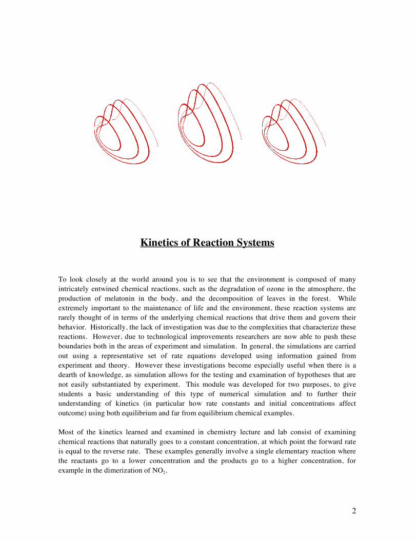
Steady State and Oscillatory Behavior

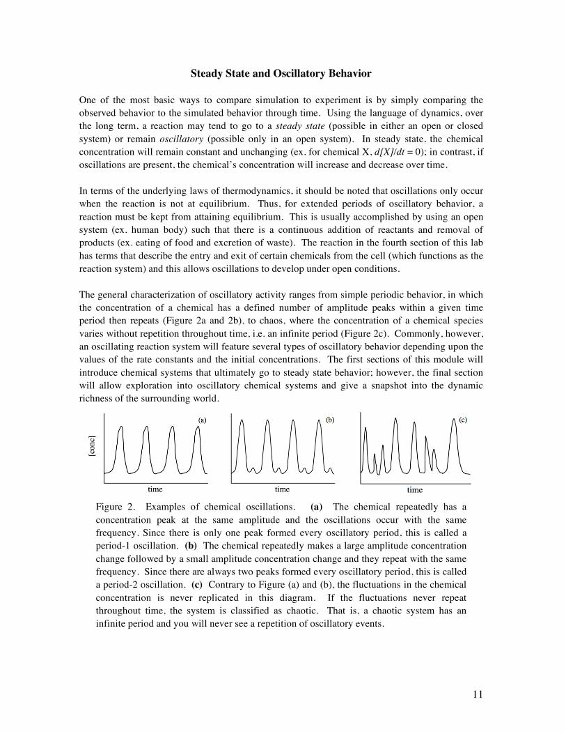
One of the most basic ways to compare simulation to experiment is by simply comparing the observed behavior to the simulated behavior through time. Using the language of dynamics, over the long term, a reaction may tend to go to a steady state (possible in either an open or closed system) or remain oscillatory (possible only in an open system). In steady state, the chemical concentration will remain constant and unchanging (ex. for chemical X, d[X]/dt = 0); in contrast, if oscillations are present, the chemical’s concentration will increase and decrease over time. In terms of the underlying laws of thermodynamics, it should be noted that oscillations only occur when the reaction is not at equilibrium. Thus, for extended periods of oscillatory behavior, a reaction must be kept from attaining equilibrium. This is usually accomplished by using an open system (ex. human body) such that there is a continuous addition of reactants and removal of products (ex. eating of food and excretion of waste). The reaction in the fourth section of this lab has terms that describe the entry and exit of certain chemicals from the cell (which functions as the reaction system) and this allows oscillations to develop under open conditions. The general characterization of oscillatory activity ranges from simple periodic behavior, in which the concentration of a chemical has a defined number of amplitude peaks within a given time period then repeats (Figure 2a and 2b), to chaos, where the concentration of a chemical species varies without repetition throughout time, i.e. an infinite period (Figure 2c). Commonly, however, an oscillating reaction system will feature several types of oscillatory behavior depending upon the values of the rate constants and the initial concentrations. The first sections of this module will introduce chemical systems that ultimately go to steady state behavior; however, the final section will allow exploration into oscillatory chemical systems and give a snapshot into the dynamic richness of the surrounding world.

Figure 2. Examples of chemical oscillations. (a) The chemical repeatedly has a concentration peak at the same amplitude and the oscillations occur with the same frequency. Since there is only one peak formed every oscillatory period, this is called a period-1 oscillation. (b) The chemical repeatedly makes a large amplitude concentration change followed by a small amplitude concentration change and they repeat with the same frequency. Since there are always two peaks formed every oscillatory period, this is called a period-2 oscillation. (c) Contrary to Figure (a) and (b), the fluctuations in the chemical concentration is never replicated in this diagram. If the fluctuations never repeat throughout time, the system is classified as chaotic. That is, a chaotic system has an infinite period and you will never see a repetition of oscillatory events.

12

Important Notes for the Use of Berkeley Madonna To simulate reaction dynamics a variety of programs may be used, examples include Berkeley Madonna, Stella and Mathematica; in this particular exercise however, guidance will be given as if you were using Berkeley Madonna. (Both a demo version and the full version can be downloaded at www.berkeleymadonna.com.) Berkeley Madonna is a suite of integration algorithms and is powerful enough to work with most reaction systems without problem. The program allows for rate equations to be input with relative ease, integrated quickly (generally seconds to minutes), and displays the output in a variety of easy to access formats (including time series, phase plane attractors, Fourier series, etc.) This program specializes in integrating rate equations and graphically presenting the simulated behavior. Your interaction with this program will be through two different interfaces, one for equation editing and for graphing. (There is also a flowchart editor, but that will not be utilized in this exercise.) In this instructional handout, the commands for the menus will be given with underlined words.

Figure 3.

A brief introduction to the programming structure of Berkeley Madonna can be found on the next page of this handout. Once the demo or full program is downloaded from the Berkeley Madonna web site (www.berkeleymadonna.com), detailed examples can be accessed through the Help menu (Help > Examples > 5 Minute Tutorial, etc.).

equation editor if not present Model > Equations

graphing interface- appears after clicking run button on equation editor

13

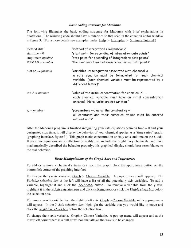
Basic coding structure for Madonna

The following illustrates the basic coding structure for Madonna with brief explanations in quotations. The resulting code should have similarities to that seen in the equation editor window in figure 3. (For a more details see examples under Help > Examples > 5 minute Tutorial.) method stiff “method of integration = Rosenbrock” starttime = 0 “start point for recording of integration data points” stoptime = number “stop point for recording of integrations data points” DTMAX = number “the maximum time between recording of data points” d/dt (A) = formula “variables -rate equation associated with chemical A --

a rate equation must be formulated for each chemical variable (each chemical variable must be represented by a different letter)”

init A = number “value of the initial concentration for chemical A --

each chemical variable must have an initial concentration entered. Note: units are not written.”

v0 = number “parameters -value of the constant v0 --

all constants and their numerical values must be entered without units”

After the Madonna program is finished integrating your rate equations between time = 0 and your designated stop time, it will display the behavior of your chemical species as a “time series” graph. (graphing interface, figure 3.) This graph marks concentration on its y-axis and time on the x-axis. If your rate equations are a reflection of reality, i.e. include the “right” key chemicals, and have mathematically described the behavior properly, this graphical display should bear resemblance to the real behavior.

Basic Manipulations of the Graph Axes and Trajectories

To add or remove a chemical’s trajectory from the graph, click the appropriate button on the bottom left corner of the graphing interface.

To change the y-axis variable, Graph > Choose Variable. A pop-up menu will appear. The Variable selection box at the left will have a list of all the potential y-axis variables. To add a variable, highlight it and click the >>Add>> button. To remove a variable from the y-axis, highlight it in the Y-Axis selection box and click <<Remove<< or click the Visible check box below the selection box.

To move a y-axis variable from the right to left axis, Graph > Choose Variable and a pop-up menu will appear. In the Y-Axis selection box, highlight the variable that you would like to move and click the Right Axis check box below the selection box.

To change the x-axis variable, Graph > Choose Variable. A pop-up menu will appear and at the lower left corner there is a pull down box that allows the x-axis to be changed.

14

Section 1 - Equilibrium

!

H2O( l ) H( aq )+

+ OH( aq )" (eq.5)

Water is one of the most amazing chemicals we encounter everyday, yet because of its abundance we often overlook its important and very unique properties. For example, it has a high specific heat that keeps the temperatures of the oceans and other large bodies of water from varying quickly, an ability to interact with microwaves in the microwave oven, etc. In this particular case however, the focus will be on water’s rare ability to act as both an acid and a base. This quality results can be seen in its capacity to autoionize (as noted in the equilibrium reaction represented by equation 5). The following questions should not only help in the understanding of rates and rate laws but should help you visualize just how fast this process is and how much of the water is converted.

Problem Set 2

1. Based on your knowledge of the world around you, do you believe that the equilibrium lies to the product or reactant side. Explain.

2. The autoionization of water is an equilibrium process and the elementary reactions are represented in equation 5. Write the associated rate laws for H2O, H+ and OH–

in the format to be used in simulations.

3. Use Berkeley Madonna to create a time series plot of the reaction (concentration versus time). Do any of the concentrations change significantly from their initial value? Does this simulation result help support or deny your assertion in question 1? Your instructor will provide a list of parameters and initial conditions to use.

4. The graph created in question 2 should show that the reaction eventually reaches and maintains steady state behavior. Circle the region on the graph that represents steady state. Explain “steady state behavior” in terms of concentration changes.

5. Explain equilibrium (that is, dynamic equilibrium) on both the macroscopic and microscopic level. How does steady state behavior relate to equilibrium?

6. Formulate a hypothesis as to how changes in the value of rate constants, kf and kr, affect such quantities as the time lapse between the initial conditions and steady state, the steady state concentrations, etc. (Assume the initial concentrations will remain the same in each trial and only the rate constants will change.)

7. Test your hypothesis with a logical set of simulations. Describe how an increase or decrease in each parameter controls such things as, time to equilibrium, steepness of concentration slope, etc. (To examine how the behavior of H2O, H+ and OH– depends on the rate constants, kf and kr , run simulations where you keep the initial concentrations the same in each trial, but allow each parameter to change individually. Examine how the simulations vary depending on whether a rate constant becomes larger or smaller.)

kf kr

15

Section 2 - Enzyme Kinetics

!

E + S ES

(eq. 6)

ES E + P

where

E = enzyme S = substrate ES = enzyme-substrate complex P = product

In this part of the module, the general reaction that represents basic enzyme-substrate interactions will be explored by simulation; these results will be compared to the initial assumptions made to understand the reaction kinetics. This model was developed in the early 1900’s to explain enzyme-catalyzed reactions such as the hydrolysis of sucrose by yeast in fermentation experiments. Since explicit integration of the rate equations is not possible, simplifying assumptions were often made that would allow a solution to be found. The two most famous simplifications were that of Michaelis and Menten (1913) and of Briggs and Haldane (1925). The supposition made by Michaelis and Menten was that the first step of the reaction reaches equilibrium and allowed determination of a solution; with further experimentation, it was later found that this idea is not often valid. Briggs and Haldane made the more generally acceptable steady state assumption; they postulated that the change in the enzyme-substrate concentration was approximately zero (d[ES]/dt = 0) for vast majority of the reaction’s lifetime. (Consult a biochemistry textbook for further details on both simplifications.) Using algorithms such as those contained within an integration suite such as Berkeley Madonna, these assumptions no longer need to be made to integrate the rate equations. Within the program, the rate equations are defined as written and the integration algorithm numerically determines a solution that is represented in the time series (or reaction progress) plots produced. The simulation results can then be used to examine which, if either, of these historical assumptions are valid in terms of your work. (1)

Problem Set 3

1. Write rate equations for the general form of enzyme substrate interaction, equation 6. You will need to form four rate equations (four ODE’s), one each for the [E], the [S], the [ES] and the [P].

2. Run a simulation and compare it to a Michaelis-Menten time series (reaction progress diagram) found in a biochemistry textbook; your simulation should look similar. Note the point at which the reaction is effectively complete and how the various concentrations change before and after that point. Your instructor will provide a list of parameters and initial conditions to use. NOTE: As it stands, this reaction is not explicitly connected to a real biochemical reaction, thus the parameters values given are not rooted in experiment or theory, the values only serve to give an illustration of enzyme-substrate behavior. If you choose to have this generalized mechanism relate to a real reaction you should use associated parameter values.

k1f k1r

k2

16

3. Explain how each rate constant, k1f , k1r , k2 affects quantities like the following: - Time to go to completion, - Amount of time where [ES] can be considered in steady state, ( d[ES]/dt ≈ 0 ) - Percentage of time spent in steady state - Steepness of concentration slopes, etc.

4. Examine how the initial concentrations of reactants (E and S) affect the quantities listed in question 2. Explain how these values, as well as the ratio of the initial concentrations, altered the simulated reaction behavior.

5. Explain the Briggs-Haldane assumption. Take a copy of a time series plot from question 4 and mark where this assumption is valid. Explain why you marked this area. What conditions (ex. large forward rate constants, certain ratios between rate constants, large initial enzyme concentration, etc.) are required for the assumption to hold true. Explain why this assumption does (or does not) give a reasonable approach to looking at a reaction that takes place in a living body, i.e. an open system.

6. Explain the Michaelis-Menten assumption. Using the same initial conditions as used in question 5, mark where this equilibrium assumption (rate forward = rate reverse) is valid. Explain why you marked this area. What conditions (ex. large forward rate constants, certain ratios between rate constants, large initial enzyme concentration, etc.) are required for the assumption to hold true. Explain why this assumption does (or does not) give a reasonable approach to looking at a reaction that takes place in a living body, i.e. an open system.

7. Enzyme substrate reactions such as the dopamine synthesis from tyrosine are found in the human body, an open reaction system. Since open systems allow for inflow and outflow of chemicals, which of the chemicals flow in, flow out or don’t flow in this type of reaction? (Use the general species designations of S, E, ES and P.) Explain how the inflow and outflow of these chemicals will affect the behavior of the system. You may support your answer with additional simulations results.

17

Section 3 - Simulations and Mechanism General chemistry books often use the nitric oxide (NO) and hydrogen (H2) reaction and its potential mechanisms to help students understand mechanisms and rate equations. In this case, you will examine if and/or how simulations can help you identify the most likely mechanistic candidate for this reaction.

!

2H2 ( g) + 2NO( g) " N2 ( g) + 2H2O( g)

Mechanism 1

H2 + NO k1# " # H2O + N (slow)

N + NO k2# " # N2 + O (fast)

O + H2 k3# " # H2O (fast)

Mechanism 2

H2 + 2NO k1# " # H2O + N2O (slow)

N2O + H2 k2# " # N2 + H2O (fast)

Mechanism 3

2NO k1f

# " # # N2O2 (fast equilibrium)

H2 + N2O2 k2# " # H2O + N2O (slow)

H2 + N2O k3# " # H2O + N2 (fast)

Problem Set 4

1. Determine rate laws for each of the three different mechanisms shown above. Run simulations of each mechanism. To facilitate the comparison between mechanisms, the values used for the initial reactant concentrations (H2 and NO)and rate constants should be identical for each simulation. (Initial concentrations for non-reactant species are zero.) Compare the resulting time series plots and describe the similarities and differences. For the differences, try to identify the differences in the reaction mechanism responsible. Your instructor will provide a list of parameters and initial conditions to use.

2. Based on this time series information, can you make a judgment as to which mechanism is most valid, i.e. most likely to represent the real mechanism? Explain your answer.

3. The simulations can give clues as to how to monitor the actual reaction to determine the real mechanism. Using simulation results how would you design experiments to distinguish between the three different mechanisms. For example, if mechanism X was valid the concentration of NO must decrease before the concentration of H2 can rise, thus by monitoring ... it should be possible to determine if this mechanism could be valid.

4. Given that the observed rate of reaction is kobs[H2][NO]2, using assumptions such as pre-equilibrium, steady state assumption, etc. which mechanism(s) is in agreement with the observed rate? (No simulations are required here.) Looking back on your answers to question 3, should it be possible to experimentally distinguish between agreeing mechanisms?

k1r

18

Section 4 - Oscillations In this section you will examine a model proposed to explain the basic mechanism behind Ca2+ oscillations in a part of the CNS. In contrast to the previous sections, you will not be asked to develop the rate equations for this reaction as the basic step-by-step mechanism is still unknown. (2-4) You will however, be given an overview as to how some researchers try to mix kinetics, biochemistry, math and simulation to help elucidate these unknown steps. To give illustration to this idea, this part of the exercise examines one of the first models proposed to explain the fundamental mechanism behind Ca2+ oscillations in astrocytes. Astrocytes are cells within the central nervous system, and it is thought that the cytosolic Ca2+ oscillations work as a signal-processing unit that allows them interact with their environment (ex. the surrounding neurons, astrocyte, etc). (3) Unfortunately, like all cells, astrocytes have many chemical reactions occurring simultaneously, and it has not been possible to experimentally determine the mechanism by which these Ca2+ oscillations are generated. To endeavor to understand the underlying mechanism, scientists are combining experimental evidence with numerical simulation. Experimentally, it has been found that Ca2+ ions within the astrocyte’s cytosol oscillate with different frequencies and patterns depending on the amount of stimulation that the cell receives from chemical neurotransmitters like glutamate. (5) The model mechanism used in this section to mimic the Ca2+ behavior was developed by Houart, et al. in 1999 (6) and, although it has been superseded by more detailed models, it was one of the earlier attempts to replicate this phenomenon in a basic way. In this model, the stimulation of the astrocyte is represented by the parameter beta, β, and it is postulated that just three interacting chemical pools are at the core of this oscillatory behavior, the Ca2+ concentration in the cytosol, the Ca2+ concentration in a storage organelle (ex. ER), and the inositol (1,4,5)-trisphosphate (IP3) concentration in the cytosol. (IP3 is a molecule produced due to the external stimulation of the cell by a neurotransmitter.) Although it is governed by only three rate equations involving [Ca2+]cyt, [Ca2+]store and [IP3], you will see that this model can exhibit a diversity of behaviors seen in observation. The general rate questions are as follows:

(eq. 7)

!

d Ca2+[ ]

cyt

dt = Ca

2+ influx from extracellular( ) " Ca

2+ efflux to extracellular( )

+ Ca2+

release from store (ex. ER)( ) " Ca2+

sequester into store (ex. ER)( )

d Ca2+[ ]

store

dt = Ca

2+ sequester into store (ex. ER)( ) " Ca

2+ release from store (ex. ER)( )

d IP3[ ]cyt

dt = production of IP3( ) " degradation of IP3( )

19

In order to be able to numerically simulate the behavior of these chemicals, the words on the right hand side of equations 7 must be replaced with physically derived values. If experimental evidence is available, this can be accomplished empirically, by fitting a mathematical formula to the experimental data. In this case, some empirical evidence was available and some intuition was used. For details regarding the development of this mechanism, see Houart et al. (6)

!

d[Ca2+]cyt

dt = v0 + v1" # v2 + v3 + k f [Ca

2+]store # k[Ca

2+]cyt

d[Ca2+]store

dt = v2 # v3 # k f [Ca

2+]store (eq. 8)

d[IP3 ]cyt

dt = "v4 # v5 # $ [IP3 ]cyt

where

v0 = constant influx of Ca2+ into the cell from the extracellular matrix β = neurotransmitter stimulation factor - values from 0 –1.0 v1 β = neurotransmitter mediated Ca2+ influx to cell from the extracellular matrix v2 = pumping rate of Ca2+ from the cytosol into the store (ex. ER)

=

!

VM 2[Ca

2+]cyt2

k22

+ [Ca2+]cyt2

"

#

$ $

%

&

' '

v3 = Ca2+ release rate from the store (ex. ER) into the cytosol

=

!

VM 3[Ca

2+]cytm

KZm

+ [Ca2+]cytm

"

#

$ $

%

&

' '

[Ca2+]store2

KY2

+ [Ca2+]store2

"

#

$ $

%

&

' '

[IP3 ]cyt4

KA4

+ [IP3 ]cyt4

"

#

$ $

%

&

' '

k [Ca2+]cyt = linear leak of Ca2+ out of the cell into the extracellular matrix kf [Ca2+]store = passive linear transport of Ca2+ out of the store (ex. ER) into the cytosol v4 = maximum rate of stimulus-induced synthesis of IP3 v5 = IP3 degradation by phosphorylation by 3-kinase

=

!

VM 5

[ IP3 ]cytp

K5p

+ [ IP3 ]cytp

"

#

$ $

%

&

' '

[Ca2+]cytn

Kdn

+ [Ca2+]cytn

"

#

$ $

%

&

' '

ε [IP3]cyt = IP3 degradation by 5-phosphatase

A full list of parameter and variable definitions, values, references, etc. can be found in Houart, et al. (6)

IP3 production IP3 degradation

to store from store

from extracellular to extracellular to store from store

20

Problem Set 5

Experimentally, Ca2+ is found to exhibit behaviors ranging from simple period-1 behavior to chaos depending upon the amount of neurotransmitter stimulation, β. Examine how varying the value of β affects the behavior of this reaction system. (When β = 0, none of the neurotransmitter receptor sites are filled, when 100% of the neurotransmitter receptor sites are filled β = 1.0.)

1. With the proper initial conditions, this model system can exhibit oscillations indefinitely. To have a chemical system where the oscillations do not cease, the system must be classified as an open system. Explain what is “the system” and what is “the surroundings” in this case. (You may find it helpful to think in terms of the biology not the chemistry and math.)

2. Explain what makes this system open and how this “openness” is demonstrated in the equations.

3. Using the parameter and initial concentration values given by your instructor, at what value of β does the oscillatory behavior start and stop.

4. Describe the oscillations that occur at the start value of β given above. (Ex. All have the same peak height, width, etc.)

5. As you move through the values of β that correspond to oscillatory behavior, do you encounter any behavior that looks chaotic? What makes you believe that this behavior is chaos?

To further support your assertion of chaos, it may help to examine the “attractor” associated with the behavior.

One way to create an attractor you is to make a plot of [Ca2+]cyt versus [Ca2+]ER. With Berkeley Madonna, do this by going to the Graph menu and click on Choose Variables… A pop-up menu will appear and at the lower left corner there is a pull down box that allows the x-axis to be changed. Change the X-axis from time to [Ca2+]ER, then click OK on the pop-up. You may have to re-run the simulation or change the zoom in order to see the attractor, which often looks like a loop of some sort.

Compare the attractor formed for what you believe is chaos and that of a more simple behavior, ex. period-1 or period-2, how are they similar/different? Do some background work to understand how attractors help to understand the type of oscillation present.

6. A commonly seen route to chaos is via a period doubling route. Explain what this route is and if it is found in this model.

7. Each of the rate equations is composed of several terms. Look at each term separately and graph their behavior as the concentrations change using a program such as Mathematica or Excel. By visualizing how the behaviors change with concentration, it should become clearer as to why certain mathematical “definitions” were used to describe a particular biological process. The following examples may be of help.

Example 1: One of the three terms in the d[IP3]/dt equation is –ε[IP3]. Since –ε[IP3] represents the degradation of IP3 by 5-phosphatase (see equation 8 for explanations) and the magnitude of the degradation is dependent on IP3 itself, it should be expected that as

21

the concentration of IP3 becomes larger it will feedback on itself and cause the [IP3] to decrease in a linear manner. (NOTE: Remember there are other factors that affect the rate of change of the [IP3], this only examines how one particular term affects d[IP3]/dt, to understand d[IP3]/dt as a whole, all three terms must be included.) Treating everything but the concentration of IP3 as a constant, graphically it will be seen that,

If experimental results show that this degradation is not a linear process, the mathematical definition would have to be changed.

Example 2: The d[Ca2+]ER/dt equation includes v2, which has the form

!

[Ca2+]cyt2

k22

+[Ca2+]cyt2

"

#

$ $

%

&

' ' .

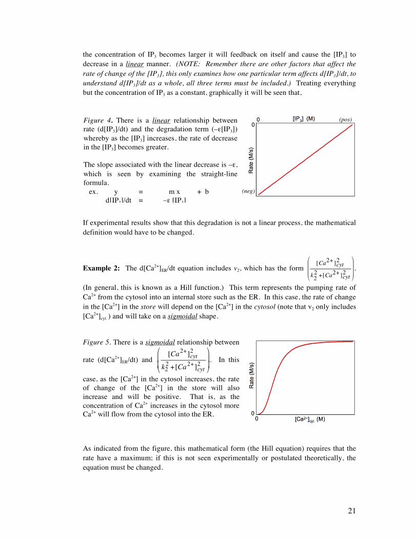
(In general, this is known as a Hill function.) This term represents the pumping rate of Ca2+ from the cytosol into an internal store such as the ER. In this case, the rate of change in the [Ca2+] in the store will depend on the [Ca2+] in the cytosol (note that v2 only includes [Ca2+]cyt ) and will take on a sigmoidal shape.

As indicated from the figure, this mathematical form (the Hill equation) requires that the rate have a maximum; if this is not seen experimentally or postulated theoretically, the equation must be changed.

Figure 4. There is a linear relationship between rate (d[IP3]/dt) and the degradation term (–ε[IP3]) whereby as the [IP3] increases, the rate of decrease in the [IP3] becomes greater. The slope associated with the linear decrease is –ε, which is seen by examining the straight-line formula. ex. y = m x + b d[IP3]/dt = –ε [IP3]

Figure 5. There is a sigmoidal relationship between

rate (d[Ca2+]ER/dt) and

!

[Ca2+]cyt2

k22

+[Ca2+]cyt2

"

#

$ $

%

&

' ' . In this

case, as the [Ca2+] in the cytosol increases, the rate of change of the [Ca2+] in the store will also increase and will be positive. That is, as the concentration of Ca2+ increases in the cytosol more Ca2+ will flow from the cytosol into the ER.

(neg)

(pos)

22

8. The Hill equation and the resulting sigmoidal form are frequently used to model biological processes such as the flow of ions through a membrane bound receptors. Why does the sigmoidal shape (as seen in figure 5) lend itself to describing process like that of ions moving through a receptor. (Think about what part of the biological process could cause an increase in rate, the maximization in rate, etc.)

9. (a) Using the Hill equation, change the values of the exponent (higher or lower) and create a figure that shows how the rate will change with respect to concentration change and change in exponent. This type of change can been seen in biological processes such as the example given in question 8. Using that example or one of your own, explain how changes in exponent could help the model more accurately reflect the process that it models. (ex. By increasing the exponent, the graphical change could indicate a given process happens at a slower rate.) (b) Using the Hill equation, change the values of the rate constant (higher or lower) and create a figure that shows how the rate will change with respect to concentration change and change in exponent. This type of change can been seen in biological processes such as the example given in question 8. Using that example or one of your own, explain how changes in exponent could help the model more accurately reflect the process it models.

Literature Cited

1. Halkides, C. J.; Herman, R., Journal of Chemical Education 2007, 84, 434-437. 2. Schuster, S.; Marhl, M.; Hofer, T., European Journal of Biochemistry 2002, 269, 1333-1355. 3. Volterra, A.; Meldolesi, J., Nature Reviews Neuroscience 2005, 6, 626-640. 4. Falcke, M., Advances in Physics 2004, 53, 255-440. 5. Cornell-Bell, A. H.; Finkbeiner, S. M.; M.S., C.; Smith, S. J., Science 1990, 247, 470-473. 6. Houart, G.; Dupont, G.; Goldbeter, A., Bulletin of Mathematical Biology. 1999, 61, 507-530. 7. Whitaker, M.; Swann, K., Development 1993, 117, 1-12.