Kinetics of a twinning step

Lifeng Liu Anna Vainchtein ∗ YangYang WangDepartment of MathematicsUniversity of PittsburghPittsburgh, PA 15260

March 13, 2013

Abstract

We study kinetics of a step propagating along a twin boundary in a cubic latticeundergoing an antiplane shear deformation. To model twinning, we consider a piece-wise quadratic double-well interaction potential with respect to one component ofthe shear strain and harmonic interaction with respect to another. We constructsemi-analytical traveling wave solutions that correspond to a steady step propaga-tion and obtain the kinetic relation between the applied stress and the velocity ofthe step. We show that this relation strongly depends on the width of the spinodalregion where the double-well potential is nonconvex and on the material anisotropyparameter. In the limiting case when the spinodal region degenerates to a point,we construct new solutions that extend the kinetic relation obtained in the earlierwork of Celli, Flytzanis and Ishioka into the low-velocity regime. Numerical sim-ulations suggest stability of some of the obtained solutions, including low-velocitystep motion when the spinodal region is sufficiently wide. When the applied stressis above a certain threshold, nucleation and steady propagation of multiple stepsare observed.

1 Introduction

Deformation twinning is a phenomenon observed in many metals and alloys. A twinboundary separates two adjacent regions of a crystal lattice that are related to one an-other by simple shear. Martensites, in particular, are known to form twinning microstruc-tures under mechanical deformation [1]. Formation and motion of twin boundaries are

∗Corresponding author, aav4@pitt.edu

1

responsible for the ability of these materials to accommodate very large deformations (upto 8-10% strain). A twin boundary propagates forward via the motion of steps, or ledges,along it [2–5]. Lattice dynamics of steps thus largely determines the macroscopic kineticsof a twin boundary [6, 7].

In this work we study the kinetics of a single step propagating along the twin bound-ary. To model this phenomenon in the simplest setting, we consider antiplane sheardeformation of a cubic lattice, with piecewise quadratic double-well interaction potentialwith respect to one component of the shear strain and harmonic interaction with respectto another. The two wells represent two different twin variants and are separated bya spinodal region where the potential is nonconvex. This is an extension of the modelwith bilinear interactions that was used in [8,9] to study high-velocity dynamics of stepsalong a phase boundary and in [10], where their quasistatic evolution was considered.Piecewise linear interactions were assumed by many authors to describe propagation ofphase boundaries, fracture and dislocations in a crystal lattice (see [11–24] and referencestherein). The advantage of such models is that they allow a semi-analytical treatmentthrough the application of Fourier transform, Wiener-Hopf technique and related meth-ods.

To find the kinetic relation between the applied stress and the velocity of the step, weneed to construct traveling wave solutions representing the steady motion of a twinningstep. The problem trivially reduces to the uniform motion of a screw dislocation studiedin [15] (see also [25,26]), where it is shown that semi-analytical solutions can be obtainedby solving a linear integral equation. The kernel of the integral equation is determinedby the solution of the problem where spinodal region degenerates into a point, which wasstudied in [13, 16]; see also [11] for a closely related one-dimensional Frenkel-Kontorova(FK) model. Despite the long history of this problem, some important questions remainedopen. One of these questions is the existence and stability of the low-velocity motion.In fact, the work in [15, 25, 26] focused primarily on solutions at some fixed velocitiesin the medium to high range and their dependence on the width of the spinodal region,while the slow propagation was not investigated. Here we use the approach in [15] toconstruct solutions for a wide range of velocities, including slow motion, and obtain theassociated kinetic relation. We show that this relation strongly depends on the width ofthe spinodal region and the material anisotropy parameter given by the relative strength ofthe harmonic bonds. We then conduct numerical simulations to independently verify someof these results and test stability of the obtained solutions. We provide semi-analyticaland numerical evidence that not only steady slow dislocation (step) motion exists, itmay become stable when the spinodal region is sufficiently wide. Unlike the high-velocitymotion, a slowly moving step requires very small stress and emits lattice waves that maypropagate both behind and ahead of the moving front. Our work thus complements andextends the results in [15,25,26]. It also extends to the higher-dimensional case the work

2

in [23], where a similar investigation was recently undertaken for the FK model.We also revisit the limiting case when the spinodal region between the two wells degen-

erates into a single point (spinodal value). In this case the earlier work [13,16] consideredtraveling wave solutions in which a transforming bond goes through the spinodal valueat a single transition point, which means that it instantaneously switches from one wellto another and remains there. While this assumption seems reasonable, it generates so-lutions only at relatively high velocities above a certain threshold value V0 (and belowanother critical velocity where the solutions break down). Below V0, the formally con-structed solutions violate the assumption used to obtain them because the transformingbond crosses the spinodal value more than once. This implies that no traveling wavesolutions of the form assumed in [13, 16] exist below the threshold value. The same non-existence result has been observed for the Frenkel-Kontorova model [11, 17]. Meanwhile,the results obtained for the models with a non-degenerate spinodal region, both the onestudied here and its FK counterpart in [23], suggest that at velocities below V0 the timeinterval during which a transforming bond remains in the spinodal region approaches anonzero value as the spinodal region shrinks to a point. This motivated the work [27] forthe FK model, where a new type of solutions below the threshold velocity was recentlyconstructed by extending the approach developed in [15] to this limiting case and allowingthe transforming bonds to stay at the spinodal value for a finite time before switchinginto another well. Here we apply this idea to the present model and show that the sameresult holds. The new solutions fill in the low-velocity gap in the kinetic relation left bythe analysis in [13,16], although, as in [27], they are likely unstable.

Finally, we investigate the solution breakdown at sufficiently high velocities when theamplitude of the lattice waves emitted by a moving step becomes sufficiently large andleads to cascade nucleation, growth and coalescence of islands on top of the existing step.The boundaries of the new islands and the initial step eventually propagate with thesame velocity. These results extend the analysis in [9] to the case with a non-degeneratespinodal region, where the island nucleation is no longer instantaneous, and support thedynamic twin nucleation and growth mechanism that was predicted in [28] and studiednumerically in [29,30].

The paper is organized as follows. Section 2 introduces the model, and the solutionprocedure is summarized in Section 3. In Section 4 we discuss the admissibility of solu-tions, obtain the kinetic relation and analyze its dependence on the width of the spinodalregion and the material anisotropy parameter. The new solutions for the case of thedegenerate spinodal region are obtained and discussed in Section 5. In Section 6 wenumerically investigate stability of the obtained solutions, and some concluding remarkscan be found in Section 7. Some additional technical results are contained in the twoAppendices.

3

2 The model

Consider a three-dimensional cubic lattice undergoing an antiplane shear deformation,which means that the atomic rows parallel to the z-direction are rigid and can onlymove along their length. Let um,n(t) denote the displacement of (m,n)th row at timet. We assume that each row interacts with its four nearest neighbors. The interactionpotentials between the neighboring rows in the horizontal and vertical directions are givenby Ψ(e) and Φ(v), where e and v denote the strains in the horizontal (m) and vertical (n)directions, respectively. The equations of motion are then given by the infinite system ofordinary differential equations:

d2

dt2um,n(t) = Ψ′(um+1,n(t)− um,n(t))−Ψ′(um,n(t)− um−1,n(t))

+ Φ′(um,n+1(t)− um,n(t))− Φ′(um,n(t)− um,n−1(t)).(1)

Here all variables are dimensionless after an appropriate rescaling [8].To model twinning, we assume that the bonds in the vertical direction are governed

by a double-well potential, with a continuous trilinear derivative:

Φ′(v) =

v + 1, v < −δ/2 (variant I)

(1− 2/δ)v, |v| ≤ δ/2 (spinodal region)

v − 1, v > δ/2 (variant II)

(2)

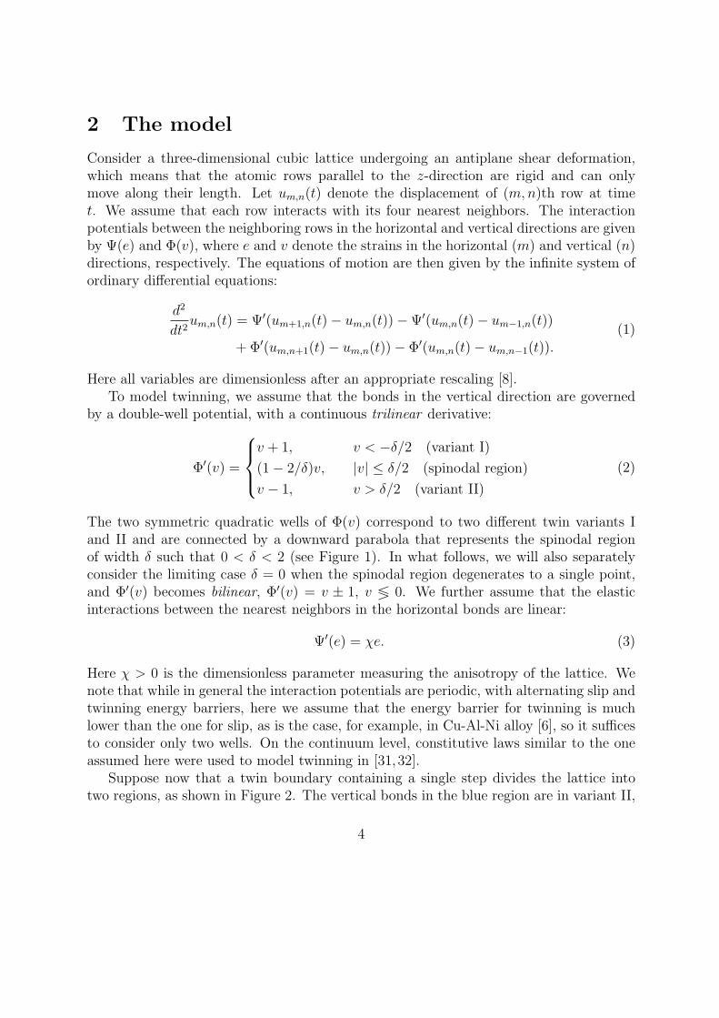
The two symmetric quadratic wells of Φ(v) correspond to two different twin variants Iand II and are connected by a downward parabola that represents the spinodal regionof width δ such that 0 < δ < 2 (see Figure 1). In what follows, we will also separatelyconsider the limiting case δ = 0 when the spinodal region degenerates to a single point,and Φ′(v) becomes bilinear, Φ′(v) = v ± 1, v ≶ 0. We further assume that the elasticinteractions between the nearest neighbors in the horizontal bonds are linear:

Ψ′(e) = χe. (3)

Here χ > 0 is the dimensionless parameter measuring the anisotropy of the lattice. Wenote that while in general the interaction potentials are periodic, with alternating slip andtwinning energy barriers, here we assume that the energy barrier for twinning is muchlower than the one for slip, as is the case, for example, in Cu-Al-Ni alloy [6], so it sufficesto consider only two wells. On the continuum level, constitutive laws similar to the oneassumed here were used to model twinning in [31,32].

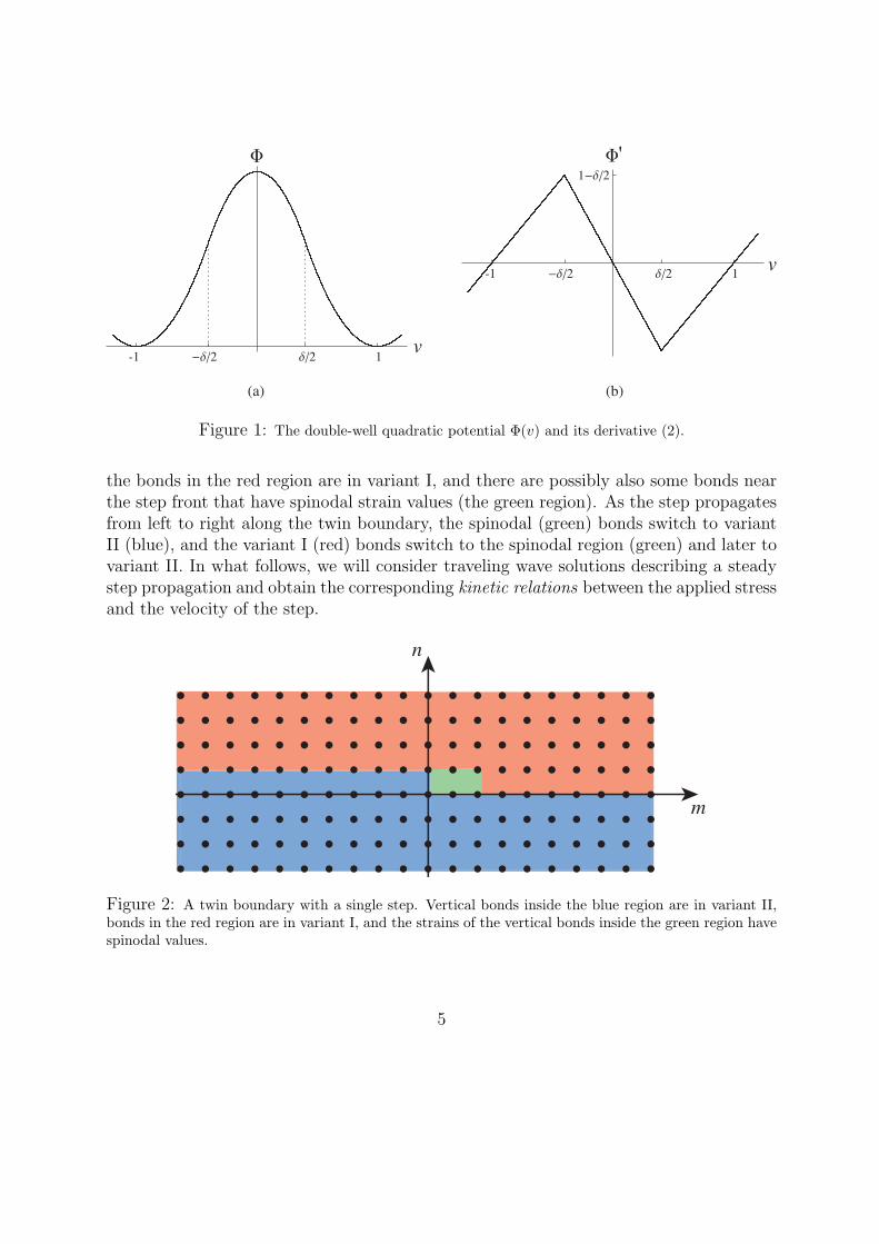
Suppose now that a twin boundary containing a single step divides the lattice intotwo regions, as shown in Figure 2. The vertical bonds in the blue region are in variant II,

4

1v

-1

1v

'

-1

(a) (b)

Figure 1: The double-well quadratic potential Φ(v) and its derivative (2).

the bonds in the red region are in variant I, and there are possibly also some bonds nearthe step front that have spinodal strain values (the green region). As the step propagatesfrom left to right along the twin boundary, the spinodal (green) bonds switch to variantII (blue), and the variant I (red) bonds switch to the spinodal region (green) and later tovariant II. In what follows, we will consider traveling wave solutions describing a steadystep propagation and obtain the corresponding kinetic relations between the applied stressand the velocity of the step.

m

n

Figure 2: A twin boundary with a single step. Vertical bonds inside the blue region are in variant II,bonds in the red region are in variant I, and the strains of the vertical bonds inside the green region havespinodal values.

5

3 Traveling wave solution

To model a steadily moving step front along the twin boundary, we seek solutions of (1)in the form of a traveling wave with (constant) velocity V > 0:

um,n(t) = u(ξ, n), ξ = m− V t. (4)

The vertical strains vm,n(t) = um,n(t)− um,n−1(t) are then given by

vm,n(t) = v(ξ, n) = u(ξ, n)− u(ξ, n− 1).

We assume that at infinity the vertical strain tends to constant values v+ < 0 and v− > 0in variant I and variant II, respectively:

v(ξ, n) → v±, as n → ±∞

v(ξ, n) →

v+, n ≥ 2

v±, n = 1

v−, n ≤ 0,

, as ξ → ±∞(5)

Furthermore, we assume the horizontal strains vanish at infinity

em,n(t) = um,n(t)− um−1,n(t) → 0, as m2 + n2 → ∞.

Note that under these assumptions and in view of (2), the applied stress is σ = v+ + 1 =v− − 1, so that

v± = σ ∓ 1. (6)

Observe also that the displacement um,n(t) is determined up to an additive constant whichcan be fixed by specifying displacement of a lattice point. As illustrated in Figure 2, weassume that the vertical bonds at n ≥ 2 and n ≤ 0 remain in their respective variants:

v(ξ, n) < −δ/2, n ≥ 2 (variant I), v(ξ, n) > δ/2, n ≤ 0 (variant II). (7)

Meanwhile, the vertical bonds at n = 1 can switch from the first to second variant as thestep propagates to the right by going through the spinodal region. Following the approachused in [15], we assume that v(ξ, 1) takes values inside the spinodal region when |ξ| < z,for some z > 0 to be determined, and is in the corresponding variant outside this interval:

v(ξ, 1) < −δ

2, ξ > z (variant I)

|v(ξ, 1)| < δ

2, |ξ| < z (spinodal region)

v(ξ, 1) >δ

2, ξ < −z (variant II),

(8)

6

and the switch between variant I (II) and the spinodal region takes place at ξ = ±z:

v(z, 1) = −δ

2, v(−z, 1) =

δ

2. (9)

Under the above assumptions we can write

Φ′(v(ξ, 1)) = v(ξ, 1) + 1− 2

∫ z

−z

θ(s− ξ)h(s)ds, (10)

where θ(s) is a unit step function: θ(s) = 1 for s > 0, θ(s) = 0 for s < 0. Here we haveintroduced an unknown shape function h(s), which is zero outside the interval [−z, z] andis normalized so that ∫ z

−z

h(s)ds = 1 (11)

Using (4), (10) and the assumed inequalities (7) and (8), we rewrite the equations ofmotion (1) as

V 2 ∂2

∂ξ2u(ξ, n) =χ (u(ξ + 1, n) + u(ξ − 1, n)− 2u(ξ, n)) + u(ξ, n+ 1) + u(ξ, n− 1)

−2u(ξ, n) + 2

[δn,0 + (δn,1 − δn,0)

∫ z

−z

h(s)θ(s− ξ)ds

] (12)

The solution of (12) can be represented as the sum of the solution of the static problemwith a flat twin boundary along n = 0 at zero stress and a solution of the dynamic problemfor a screw dislocation located at the step front and moving steadily under the appliedstress. More precisely, we write

u(ξ, n) = uFn + w(ξ, n), (13)

where

uFn =

0, n ≥ 0

2n, n ≤ −1(14)

satisfies the static flat-boundary problem

uFn+1 + uF

n−1 − 2uFn + 2δn,0 = 0, (15)

and the screw dislocation solution is given, up to an additive constant, by [15]

w(ξ, n) = n(σ − 1) +1

2π2

∫ ∞

−∞

e−ikξξH(kξ)J (kξ, n)

i(kξ − i0)dkξ. (16)

7

Here kξ − i0 = limε→0+(kξ − iε), H(kξ) is the Fourier transform of h(x) and

J (kξ, n) =

∫ π

−π

(1− eiky)e−inky

V 2k2ξ − 4(χ sin2 kξ

2+ sin2 ky

2)dky (17)

is defined for integer n. The integral in (17) can be explicitly calculated using the residuetheorem, yielding (41) in the Appendix A. Using (13), (14), (16) and the convolutionproperties of the Fourier transform, we obtain the vertical strains in the lattice as

v(ξ, n) =

∫ z

−z

g|n−1|(ξ − s)h(s)ds+

σ − 1, n ≥ 1

σ + 1, n ≤ 0.(18)

Here we defined

gj(ξ) =1

π

∫ ∞

−∞

e−ikξξ

i(kξ − i0)S(kξ, j)dkξ, j = 0, 1, 2, . . . , (19)

where

S(kξ, j) =

(λ−

√λ2 − 1)−|j|(δj,0 −

√λ−1λ+1

), λ < −1

(λ∓ i√1− λ2)−|j|(δj,0 ± i

√1−λ1+λ

), |λ| < 1, kξ ≶ 0

(λ+√λ2 − 1)−|j|(δj,0 −

√λ−1λ+1

), λ > 1

(20)

and

λ(kξ) = 1 + 2χ sin2 kξ2

− 1

2V 2k2

ξ . (21)

Observe now that on one hand, we have

∂

∂ξv(ξ, 1) = −

∫ z

−z

q(ξ − s)h(s)ds, (22)

where, by (18) and (19),

q(ξ) = −g′0(ξ) =1

π

∫ ∞

−∞e−ikξξS(kξ, 0)dkξ. (23)

On the other hand, (2) and (10) imply that for |ξ| < z

v(ξ, 1) = δ

(∫ z

ξ

h(s)ds− 1

2

),

and thus∂

∂ξv(ξ, 1) = −δh(ξ). (24)

8

Together, (22) and (24) yield a Fredholm integral equation of the second kind [15]:∫ z

−z

q(ξ − s)h(s)ds = δh(ξ), |ξ| < z, (25)

where the shape function h(ξ) is an eigenfunction of the integral operator in the left handside of (25) with kernel (23) associated with the eigenvalue δ. The problem thus reducesto solving the integral equation (25) for z and h(ξ).

Once h(ξ) and z are known, the vertical strains for the traveling wave solution canbe computed from (18). Substituting (18) into the switch conditions (9) and subtractingthe first condition from the second, we obtain

∫ z

−z(g0(−z − s) − g0(z − s))h(s)ds = δ,

which is automatically satisfied, as can be verified by integrating (25) and recalling (11)and the first equality in (23). Meanwhile, adding the two conditions yields the followingexpression for the applied stress:

σ = 1− 1

2

∫ z

−z

h(s)[g0(z − s) + g0(−z − s)]ds. (26)

Since g0 depends on V , this defined the kinetic relation σ = Σ(V ) between the appliedstress σ and the step moving velocity V . The relation also depends on δ and χ.

We remark that the real wave numbers kξ such that |λ(kξ)| ≤ 1, with λ given by(21), correspond to the lattice waves emitted by the moving step because this inequalityimplies the existence of real wave numbers ky such that the velocity of the moving stepequals the horizontal component of the phase velocity of some plane waves: V = ω/kξ,where ω2 = 4(χ sin2(kξ/2) + sin2(ky/2)) is the dispersion relation [13]. One can show [15]that only these waves, which carry energy away from the step, contribute to the stressin (26). The transfer of energy from long (continuum level) to short (lattice-scale) wavesassociated with this nonlinearity-induced radiation is known in the physics literature asthe radiative damping phenomenon (e.g. [17]).

It should be emphasized that the solutions of (12) satisfy the original nonlinear equa-tion (1) if and only if the admissibility conditions (7) and (8) hold. Solutions of (12) thatviolate any of the admissibility conditions will be called inadmissible.

4 Admissible solutions and kinetic relations

We first review the limiting case z = 0 that reduces to the screw dislocation problemstudied in [15, 16]. One can see that in this limit we must have δ = 0, i.e. spinodalregion degenerates to a single point and Φ′(v) becomes bilinear, while the shape functionbecomes a Dirac delta function: h(s) = δD(s). Thus, (18) reduces to

v0(ξ, n) = u0(ξ, n)− u0(ξ, n− 1) = g|n−1|(ξ) +

σ − 1, n ≥ 1

σ + 1, n ≤ 0, (27)

9

where u0(ξ, n) satisfies

V 2 ∂2

∂ξ2u0(ξ, n) = χ(u0(ξ + 1, n) + u0(ξ − 1, n)− 2u0(ξ, n)) + u0(ξ, n+ 1) + u0(ξ, n− 1)

−2u0(ξ, n) + 2 [δn,0 + (δn,1 − δn,0)θ(−ξ)] .

(28)

We observe that the first equality in (23) and (27) imply that

q(ξ) = −∂v0(ξ, 1)

∂ξ. (29)

Note that the vertical strain v0(ξ, n) should also satisfy the corresponding admissibilityconditions (7) and (8) at z = 0 and δ = 0, which reduce to (with v = v0)

v(ξ, n) < 0, n ≥ 2 (variant I), v(ξ, n) > 0, n ≤ 0 (variant II). (30)

andv(ξ, 1) < 0, ξ > 0 (variant I), v(ξ, 1) > 0, ξ < 0 (variant II), (31)

respectively. The kinetic relation (26) can be shown in this case to yield σ = Σ0(V )defined by

σ = 1− g0(0) =2

π

∫ ∞

0

1

kξ

√1− λ(kξ)

1 + λ(kξ)θ(1− |λ(kξ)|)dkξ, (32)

where we recall that λ(kξ) is given by (21). The reader is referred to [8, 13, 16] for moredetails.

The resulting kinetic relation, shown in Figure 3a, consists of disjoint segments sep-arated by resonance velocities, i.e. values of V such that λ(kξ) = −1 and λ′(kξ) = 0 forsome real kξ (see Figure 3b). At these velocities the kinetic relation has either a loga-rithmic singularity (at the resonance velocities that correspond to the local minima ofV (kξ) such that λ = −1) or a jump discontinuity (at the local maxima) [16]. A typicaladmissible solution (V = 0.5) above the first resonance V1 ≈ 0.3158 is shown in Fig-ure 4a. One can see that the moving step generates lattice waves behind it. As velocitydecreases below the first resonance, solution develops oscillations at ξ > 0 as well; see, forexample, the vertical strain profile at V = 0.17 in Figure 4b, where two modes of emittedlattice waves propagate behind and one mode ahead of the step. However, a closer in-spection reveals that this solution is in fact inadmissible and should be removed becauseit violates the first inequality in both (30) and (31). At χ = 1, our calculations showthat the large-velocity segment contains admissible solutions above a certain threshold,V ≥ V0 ≈ 0.4649, while in several segments of the kinetic relation below the threshold,

10

we only found inadmissible traveling waves that violate (31) and sometimes also (30), andthus need to be removed. This suggests non-existence of traveling wave solutions with ve-locity lower than the threshold value in the z = 0 case, in agreement with the conjecturesmade in [13, 16]. Meanwhile, solutions at sufficiently high velocities (V ≥ Vh ≈ 0.9908 atχ = 1) are also inadmissible, because the large amplitude of waves propagating behindthe step front causes the n = 2 bonds directly above the step to switch from variant I tovariant II, which violates the first inequality in (30) (see also [8]).

10 20 30 40

0.1

0.2

0.3

0.4

0.5

0.6

0.2 0.4 0.6 0.8 1.0

0.5

1.0

1.5

s

V kx

V

(a) (b)

Figure 3: (a) Kinetic relation σ = Σ0(V ) at z = 0, δ = 0. Only the first twenty segments areshown. Admissible solutions correspond to the dark portion of the first segment. (b) Velocities V suchthat λ = −1 for positive real kξ. The dashed lines indicate the first five resonance velocities at whichλ(kξ) = −1 and λ′(kξ) = 0. Here χ = 1.

Consider now the trilinear problem with δ > 0. To find h(s) and z for given non-resonant V > 0 and δ > 0, we approximate the integral equation (25) by a trapezoidalrule with an uniform mesh, obtaining a homogeneous linear system (Q(z) − δI)h = 0,where Q(z) is the matrix approximating the integral operator, I is the identity matrix,and h is the vector approximating the unknown shape function. To find z, we solve thenonlinear algebraic equation det(Q(z) − δI) = 0, which ensures that δ is an eigenvalueof Q(z), and then find the corresponding eigenvector h, normalized by (11). In general,there may be more than one value of z but our calculations suggest that at most onevalue yields admissible solutions. Once z and h are found, the trapezoidal approximationof the integrals in (18) and (26) is used to compute the solution v(ξ, n) and the appliedstress σ.

The resulting vertical strains of n = 1 and n = 2 bonds at V = 0.17 are shown byFigure 5 for δ = 0.8 (which yields z = 0.424 and σ = 0.0409) and δ = 1.2 (z = 0.875and σ = 0.0039). As in [15], we observe that the main effect of increasing δ, which leadsto larger z, is the decreased amplitude of the oscillations due to wave modulation that

11

-6 -4 -2 2 4

-1.0

-0.5

0.5

1.0n=1

n=2

n=1

n=2

v0

x x

(a) V=0.5 (b) V=0.17

-6 -4 -2 2 4

-1.0

-0.5

0.5

1.0

1.5

v0

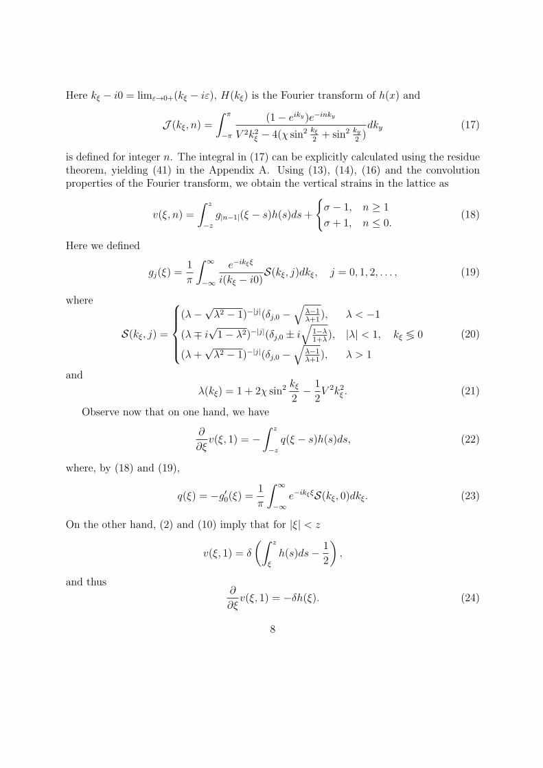
Figure 4: Vertical strain v0(ξ, n) profiles at n = 1, 2 formally computed from (27) and (32) at z = 0,δ = 0, χ = 1 and velocities (a) V = 0.5 (σ = 0.2096) and (b) V = 0.17 (σ = 0.5736). Solution in(a) satisfies the constraints (30) and (31) but the one in (b) violates both constraints at ξ > 0. Hereand in the pictures below n = 0 strains are not shown because by the symmetry of g|n−1|(ξ) and (18),v(ξ, 0) = v(ξ, 2) + 2.

takes place over the larger time interval. As a result, the solutions at V = 0.17 becomeadmissible at δ = 0.8 and δ = 1.2, while the corresponding solution of the bilinear problemat z = 0 is not. Note also that the stress decreases as δ is increased due to the smallercontribution of the lattice waves, although it may oscillate at larger values of δ [25, 26].

Figure 6 shows the half-width z of the transition region as a function of V for differentδ at χ = 1, and the corresponding kinetic relations are shown in Figure 7. Due the pile-upof resonance velocities as V approaches zero, which makes the computation progressivelymore difficult, only V ≥ 0.1 were considered. A detailed inspection suggests that allsolutions shown except the ones along the grey portions of the curves are admissible. Thisincludes solutions in the immediate vicinity of the resonance velocities, which correspondto the cusps in Figure 6 and Figure 7. Note that the kinetic relations are highly non-monotone, with larger stress variations at lower δ. Observe also that at δ = 1.2 thelow-velocity motion requires very little applied stress, due to the small amplitude of theemitted waves and thus small amount of radiative damping. This “solitonlike” dislocationbehavior is discussed in [25,26].

Interestingly, as in [23], our numerical calculations reveal that as δ approaches zeroat velocities below the threshold value V0 ≈ 0.4649, the value of z approaches a positivevalue rather than zero, contrary to the assumption of z = 0 in [13,16] for the bilinear case.This motivates us to construct a new type of traveling wave solutions for the limiting caseδ = 0 that has z > 0 below the threshold value. We postpone the discussion of these

12

-6 -4 -2 2 4

-1.0

-0.5

0.5

1.0

-6 -4 -2 2

-1.0

-0.5

0.5

1.0

n=1

n=2

n=1

n=2

(a) d=0.8 (b) d=1.2

v

x

v

x

v=d/2

v=-d/2

v=d/2

v=-d/2

4

Figure 5: Vertical strain v(ξ, n) (n = 1, 2) profiles at V = 0.17, with (a) δ = 0.8 (z = 0.424, σ = 0.0409)and (b) δ = 1.2 (z = 0.875, σ = 0.0039). Both solutions are admissible. Here χ = 1.

0.2 0.4 0.6 0.8 1.0

0.5

1.0

1.5

2.0

2.5

0.1 0.2 0.3 0.40.0

0.1

0.2

0.3

0.4

z z

V V

d=1.2

d=0.8

d=0.4

d=0

d=0

d=0.4

d=0.8

(a) (b)

Figure 6: (a) The half-width z(V ) of the transition region for different δ calculated for V ≥ 0.1. (b)Zoom-in of the small-velocity region inside the rectangle. Here χ = 1. The thicker black segments containadmissible solutions, while the gray segments correspond to inadmissible solutions.

13

0.2 0.4 0.6 0.8 1.0

0.2

0.4

0.6

0.10 0.15 0.20 0.25 0.30

0.01

0.02

0.03

0.04

0.05

s

V

s

V

(a) (b)

d=1.2

d=0.8

d=0.4

d=0

d=0.8

d=1.2

Figure 7: (a) Kinetic relations σ = Σ(V ) for different δ and V ≥ 0.1. (b) Zoom-in of the small-velocityregion inside the rectangle. Here χ = 1. The thicker black segments contain admissible solutions, whilethe gray segments correspond to inadmissible solutions.

new solutions until Section 5, while here we simply show the corresponding curves forcomparison.

We now consider the dependence of the kinetic relation σ = Σ(V ) on χ, the dimension-less anisotropy parameter measuring the shear strength of the linearly elastic horizontalbonds relative to the vertical ones. Let c =

√χ be the sound speed of elastic shear waves

in the horizontal direction of the step motion. At δ = 0.8, typical kinetic relations atdifferent χ are shown in Figure 8b, and the corresponding z(V ) graphs in Figure 8a. Notethat the resonance velocities take different values for different χ, so the locations of thecusps in the kinetic relation changes. One can see that a higher χ results in a lowerapplied stress at the same normalized velocity V/c because it means a stronger couplingof the vertical bonds.

At sufficiently large velocities above a threshold Vh (for example, V > Vh ≈ 0.9389at δ = 0.8 and χ = 1), the amplitude of the waves propagating behind the step frontbecomes so large that strain in some n ≥ 2 bonds above the step enters the spinodal regionfrom variant I, violating the first constraint in (7) and thus rendering the correspondingsolutions inadmissible (see the gray large-velocity segments in Figures 6a, 7a and 8). Onecan observe that at χ = 1 the upper threshold Vh increases as δ decreases. Meanwhile,at the same δ = 0.8, the normalized upper threshold Vh/c increases as χ is increased. Aswe will see in Section 6, this solution failure at σ > σh = Σ(Vh) corresponds to a cascadenucleation of new steps.

In addition to the traveling wave solutions, there are equilibrium states (V = 0) thatexist when the applied stress is in the trapping region |σ| ≤ σP , where σP is the Peierlsstress (51). One can show [33] that at 0 < δ < 2 there are two equilibrium states with theassumed single-step configuration for |σ| < σP , a stable state with ms spinodal vertical

14

0.2 0.4 0.6 0.8 1.0

0.5

1.0

0.2 0.4 0.6 0.8 1.0

0.1

0.2

0.3

0.4

0.5

c=0.5

c=1

c=2

c=2

c=1

c=0.5

z s

V/c V/c

(a) (b)

Figure 8: (a) The half-width z(V ) of the transition region and (b) kinetic relations σ = Σ(V ) at differentχ. The thicker black segments contain admissible solutions, while the gray segments corresponding toinadmissible solutions. Here δ = 0.8, and the velocities are normalized by c =

√χ.

bonds near the step front and an unstable state with ms + 1 spinodal bonds, where ms

and σP determined by δ and χ (see Appendix B for more details). These solutions aregiven by (46) for ms = 0 and (49), (50) for ms ≥ 1.

5 New traveling wave solutions

We now revisit the bilinear problem (δ = 0) with degenerate spinodal region, where, aswe recall, no admissible solutions were found for V < V0 at z = 0. However, as we alreadymentioned above, our results for small δ in this velocity region suggest that z tends to anonzero value as δ approaches zero. This suggests that following the approach recentlypursued for the one-dimensional problem [27], we should seek solutions with z > 0 andreplace the admissibility conditions (31) by the more general conditions

v(ξ, 1) < 0, ξ > z (variant I),

v(ξ, 1) = 0, |ξ| ≤ z (degenerate spinodal region),

v(ξ, 1) > 0, ξ < −z (variant II),

(33)

while leaving (30) (or, equivalently, (7) at δ = 0) the same. Note that (9) at δ = 0 isincluded in (33), so we seek solutions of (12) subject to (30) and (33).

Observe now that (22) still holds. At the same time, our assumption that v(ξ, 1) ≡ 0at |ξ| ≤ z implies ∂

∂ξv(ξ, 1) ≡ 0 in the interval (−z, z). Together with (22), this yields a

Fredholm integral equation of the first kind:∫ z

−z

h(s)q(ξ − s)ds = 0 |ξ| < z. (34)

15

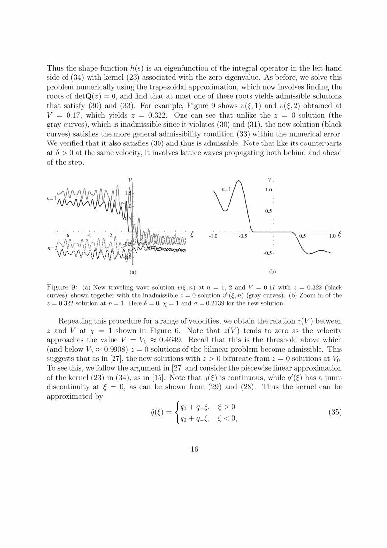
Thus the shape function h(s) is an eigenfunction of the integral operator in the left handside of (34) with kernel (23) associated with the zero eigenvalue. As before, we solve thisproblem numerically using the trapezoidal approximation, which now involves finding theroots of detQ(z) = 0, and find that at most one of these roots yields admissible solutionsthat satisfy (30) and (33). For example, Figure 9 shows v(ξ, 1) and v(ξ, 2) obtained atV = 0.17, which yields z = 0.322. One can see that unlike the z = 0 solution (thegray curves), which is inadmissible since it violates (30) and (31), the new solution (blackcurves) satisfies the more general admissibility condition (33) within the numerical error.We verified that it also satisfies (30) and thus is admissible. Note that like its counterpartsat δ > 0 at the same velocity, it involves lattice waves propagating both behind and aheadof the step.

-6 -4 -2 2 4

-1.0

-0.5

0.5

1.0

1.5

-1.0 -0.5 0.5 1.0

-0.5

0.5

1.0

(a) (b)

v

x

v

x

n=1

n=2

n=1

Figure 9: (a) New traveling wave solution v(ξ, n) at n = 1, 2 and V = 0.17 with z = 0.322 (blackcurves), shown together with the inadmissible z = 0 solution v0(ξ, n) (gray curves). (b) Zoom-in of thez = 0.322 solution at n = 1. Here δ = 0, χ = 1 and σ = 0.2139 for the new solution.

Repeating this procedure for a range of velocities, we obtain the relation z(V ) betweenz and V at χ = 1 shown in Figure 6. Note that z(V ) tends to zero as the velocityapproaches the value V = V0 ≈ 0.4649. Recall that this is the threshold above which(and below Vh ≈ 0.9908) z = 0 solutions of the bilinear problem become admissible. Thissuggests that as in [27], the new solutions with z > 0 bifurcate from z = 0 solutions at V0.To see this, we follow the argument in [27] and consider the piecewise linear approximationof the kernel (23) in (34), as in [15]. Note that q(ξ) is continuous, while q′(ξ) has a jumpdiscontinuity at ξ = 0, as can be shown from (29) and (28). Thus the kernel can beapproximated by

q(ξ) =

q0 + q+ξ, ξ > 0

q0 + q−ξ, ξ < 0,(35)

16

whereq0 = q(0), q± = q′(0±), q+ − q− = 4/V 2, (36)

with the last relation is implied by (28) and (29). Solving the approximate version of(34), i.e.

∫ z

−zh(s)q(ξ − s)ds = 0, |ξ| < z, one obtains [27]

z =q0(q+ − q−)

2q+q−(37)

andh(ξ) =

q−q− − q+

δD(ξ + z)− q+q− − q+

δD(ξ − z), (38)

in the sense of distributions. Numerical evaluation of (23) and the last of (36) show that(q+ − q−)/(2q+q−) < 0 when V is near the threshold V0. Thus the positive solution zgiven by (37) exists provided that −q0 = ∂

∂ξv0(0, 1) > 0. Meanwhile, the admissibility

conditions (31) imply that ∂∂ξv0(0, 1) ≤ 0. This indicates that bifurcation of the new

type of traveling wave with z > 0 occurs precisely at the threshold velocity V0, at whichq0(V0) = 0, and below which the z = 0 solution are inadmissible because (31) is violated.As shown in Figure 10, the values of z(V ) obtained from the numerical solution of (34)with the original kernel (23) near the threshold velocity V0 approach the values (37)resulting from the linear approximation near the threshold velocity.

0.450 0.452 0.454 0.456 0.458 0.460 0.462 0.464

0.002

0.004

0.006

0.008

0.010

0.012

0.014

0.450 0.452 0.454 0.456 0.458 0.460 0.462 0.464

0.00005

0.00010

0.00015

0.00020

0.00025

V V

zL

zN

zN-zL

(a) (b)

Figure 10: Comparison of the function zN (V ) computed numerically using the kernel (23) (solid line)and zL(V ) obtained from (37) using the linear approximation (35) of the kernel (dashed line) near thebifurcation point V0 ≈ 0.4649.

The corresponding kinetic relation σ = Σ(V ) is shown in Figure 7. It coincides withthe z = 0 relation Σ0(V ) above the velocity V0, while below this threshold, where z > 0,it provides lower values of the applied stress and replaces the singularities in Σ0(V ) at

17

0.1 0.2 0.3 0.40.0

0.2

0.4

0.6

0.8

1.0

1.2

s

V

Figure 11: Comparision of the kinetic relation σ = Σ(V ) generated by the new solutions with z > 0with the relation Σ0(V ) obtained from the formal z = 0 solutions of the bilinear (δ = 0) problem. Thetwo curves coincide above the threshold velocity V0 ≈ 0.4649. The gray curves correspond to inadmissiblez = 0 solutions below V0.

the resonance velocities by cusps; see Figure 11 for comparison. This result thus extendsthe kinetic relation obtained in [13,16] for δ = 0 case into the region of velocities V < V0,where the new solutions with z > 0 “fill the gap” left by the non-existence of admissiblesolutions with z = 0.

6 Stability of the traveling waves: numerical simula-

tions

To investigate stability of the obtained traveling waves solutions and obtain an indepen-dent verification of our results, we solve the equations (1) numerically without assumingany particular motion pattern and then compare the numerical results with the travelingwave solutions. We use the velocity Verlet algorithm in the computational domain Ωgiven by a truncated 400 × 8 lattice. The initial configuration has a flat twin boundarywith a single step in the center of the domain, as in Figure 2. To avoid reflection of latticewaves from the boundary of Ω, we use the non-reflective boundary conditions (NRBC)developed in [9]. Assuming that the initial condition outside the computational domainsatisfies the equilibrium equations with zero initial velocity and that the problem thereremains linear (i.e. the vertical bonds remain in their respective variants), the NRBCconditions prescribe the displacement on ∂Ω+, a set of lattice points outside the compu-tational domain Ω that have at least one nearest neighbor belonging to ∂Ω, the boundaryof Ω.

18

To construct the initial condition for given δ and applied stress below the Peierlsthreshold, 0 < σ < σP , we start with an equilibrium state (stable or unstable), given by(46) if there are no spinodal bonds and (49), (50) if there is at least one such bond. Totrigger step propagation, we perturb this state by changing the vertical strain in front ofthe step. Above the Peierls threshold, no equilibrium state exists but we use the sameformulas to ensure that the initial state satisfies the equilibrium equations outside Ω, asrequired by the NRBC conditions we use. Inside the computational domain, this yields anon-equilibrium displacement. If it does not satisfy the assumed initial phase distribution,we modify the initial displacement in Ω by prescribing strains in some vertical bonds andsolving a constrained equilibrium problem that ensures the assumed inequalities hold.Initial velocities are set to zero.

We find that for sufficiently small σ below the Peierls threshold the numerical solutiongets trapped in a stable equilibrium state. For higher applied stress, the step propagates,and after some transient time its motion becomes steady, which means that the timeperiod during which the front moved from one vertical bond in the lattice to the nextapproaches a constant value T . The velocity is then obtained by computing V = 1/T asthe average over the last ten periods.

Figures 12 and 13 compare (V , σ) obtained from the numerical results (circles) forδ = 1.2 and δ = 0.8 (at χ = 1) with the corresponding semi-analytical kinetic relationcurves. One can see that the numerical results are in very good agreement with someincreasing portions of the kinetic curves, which suggests stability of the traveling wavesolutions with the corresponding velocities. The fact that the numerical results only fall

0.2 0.4 0.6 0.8 1.0

0.1

0.2

0.3

0.1 0.2 0.3 0.4 0.50.000

0.005

0.010

0.015

s

V

s

V

(a) (b)

sP

Figure 12: (a) Results of the numerical simulations for δ = 1.2 (circles), shown together with the kineticcurve. (b) Zoom-in of the small-velocity region inside the rectangle in (a).

on the increasing portions of the curves supports the conjecture in [23] that Σ′(V ) > 0is necessary but not sufficient for stability. Note, in particular, that the results indicate

19

0.2 0.4 0.6 0.8 1.0

0.1

0.2

0.3

0.4

0.5

0.05 0.10 0.15 0.20 0.25 0.30 0.350.035

0.040

0.045

0.050

0.055

0.060

0.065

s

V

s

V

(a) (b)

sP

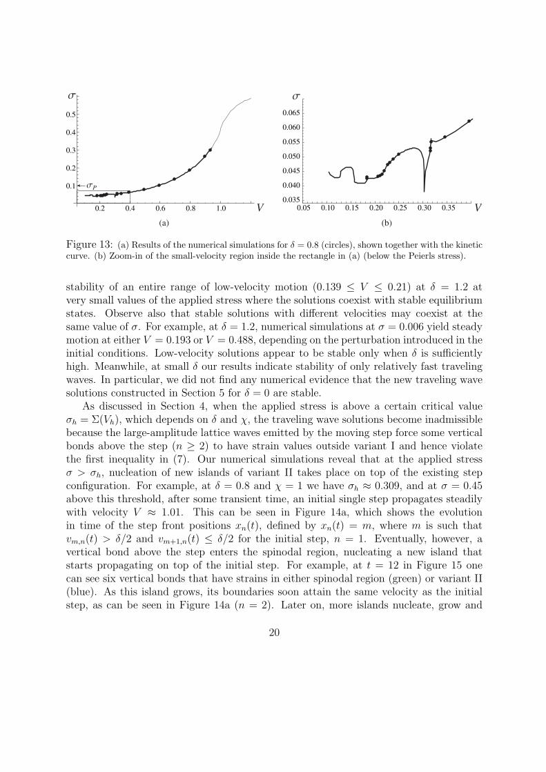
Figure 13: (a) Results of the numerical simulations for δ = 0.8 (circles), shown together with the kineticcurve. (b) Zoom-in of the small-velocity region inside the rectangle in (a) (below the Peierls stress).

stability of an entire range of low-velocity motion (0.139 ≤ V ≤ 0.21) at δ = 1.2 atvery small values of the applied stress where the solutions coexist with stable equilibriumstates. Observe also that stable solutions with different velocities may coexist at thesame value of σ. For example, at δ = 1.2, numerical simulations at σ = 0.006 yield steadymotion at either V = 0.193 or V = 0.488, depending on the perturbation introduced in theinitial conditions. Low-velocity solutions appear to be stable only when δ is sufficientlyhigh. Meanwhile, at small δ our results indicate stability of only relatively fast travelingwaves. In particular, we did not find any numerical evidence that the new traveling wavesolutions constructed in Section 5 for δ = 0 are stable.

As discussed in Section 4, when the applied stress is above a certain critical valueσh = Σ(Vh), which depends on δ and χ, the traveling wave solutions become inadmissiblebecause the large-amplitude lattice waves emitted by the moving step force some verticalbonds above the step (n ≥ 2) to have strain values outside variant I and hence violatethe first inequality in (7). Our numerical simulations reveal that at the applied stressσ > σh, nucleation of new islands of variant II takes place on top of the existing stepconfiguration. For example, at δ = 0.8 and χ = 1 we have σh ≈ 0.309, and at σ = 0.45above this threshold, after some transient time, an initial single step propagates steadilywith velocity V ≈ 1.01. This can be seen in Figure 14a, which shows the evolutionin time of the step front positions xn(t), defined by xn(t) = m, where m is such thatvm,n(t) > δ/2 and vm+1,n(t) ≤ δ/2 for the initial step, n = 1. Eventually, however, avertical bond above the step enters the spinodal region, nucleating a new island thatstarts propagating on top of the initial step. For example, at t = 12 in Figure 15 onecan see six vertical bonds that have strains in either spinodal region (green) or variant II(blue). As this island grows, its boundaries soon attain the same velocity as the initialstep, as can be seen in Figure 14a (n = 2). Later on, more islands nucleate, grow and

20

0 10 20 30 40 500

20

40

60

80

100

t 0 5 10 15 20 25 30 35 400

20

40

60

80

100

t

(a) s=0.45 (b) s=0.55

n=1

n=2

xn xn

n=3

n=3

n=4

Figure 14: Evolution of step front positions xn(t) during island nucleation, propagation and coalescenceat different values of the applied stress above the threshold value σh. Here δ = 0.8 and χ = 1.

coalesce, and all the fronts eventually propagate with the same velocity; see Figure 14aand Figure 15. At higher applied stress, σ = 0.55, island nucleation occurs sooner, andnew islands nucleate and merge more frequently. While these observations are similarto the results obtained in [9] for a potential with a degenerate spinodal region, the newfeature here is that island nucleation no longer occurs instanteneously but requires sometime to develop. For example, the right island at n = 3 in Figure 15 starts forming alreadyaround t = 29, where one can see a bond inside the spinodal region, but it does not fullydevelop and start growing until a much later time, as can be seen from t = 42 snapshot,where the island has only grown by a few bonds (see also Figure 14). The cascade islandnucleation observed here is in agreement with the dynamic twin nucleation and growthdue to lattice waves emitted by a sufficiently fast motion of a screw dislocation that waspredicted in [28] and studied numerically in [29] and [30].

7 Concluding Remarks

In this work, we used a simple antiplane shear lattice model with piecewise linear inter-actions to study the motion of a step propagating along a twin boundary. Following theapproach developed in [15], we constructed semi-analytical traveling wave solutions fora wide range of the velocities and showed that the width of the spinodal region and thematerial anisotropy have a significant effect on the resulting kinetic relation between theapplied stress and the velocity of the step. Our results extend and complement the work

21

t = 0

t = 12

t = 29

t = 42

t = 50

t = 54

Figure 15: Time snapshots of island nucleation and growth at σ = 0.45, δ = 0.8 and χ = 1. Thecorresponding evolution of step fronts is shown in Figure 14a. Here the blue points represent verticalbonds that have strain in variant II, the red ones are in variant I, and the green ones are in the spinodalregion.

22

in [15, 25, 26] by considering slow step propagation that was not previously investigated.Our semi-analytical results and numerical simulations strongly suggest that such motiondoes not only exist but may become stable if the spinodal region is sufficiently wide.The slow step motion requires very small applied stress and involves emitted lattice wavethat may propagate both behind and ahead of the moving step. This is in contrast tothe previously studied high-velocity motion that feature waves only behind the step andrequires a larger stress. We also numerically investigated the solution breakdown whenthe applied stress is above a certain critical value. In this case the lattice waves emittedby the moving step and propagating behind it enter the spinodal region and lead to acascade nucleation, growth and coalescence of multiple islands on top of the moving step.Compared to the similar results in [9], where the spinodal region was degenerate, in ourcase the island nucleation does not happen instantaneously.

The solution procedure was also used to find new admissible traveling wave solutions atlow velocities in the case when the spinodal region degenerates to a single point. Applyingthe method in [27], we showed that these new solutions, in which the transforming bondsstay at the spinodal value before switching to the new twin variant, bifurcate from thesolutions where the transition is instantaneous precisely at the threshold velocity wherethe latter become inadmissible. This allowed us to extend the kinetic relation in [13, 16]to lower velocities, where no admissible solutions were previously found.

We remark that the kinetic relations obtained here are in general quantitatively dif-ferent from the ones obtained in [23, 27] for the closely related one-dimensional Frenkel-Kontorova model due to the different kernel (23) in the integral equation (25). In par-ticular, the amplitude of the oscillations in our kernel decays at infinity [8], while in theone-dimensional case it remains constant. Note also that the one-dimensional problemhas stronger singularities at the resonance velocities in the z = 0 case [16]. Nevertheless,qualitatively many of the results are similar, suggesting that the one-dimensional model,which is technically much less involved, captures the basic features of the kinetics of asingle step. One important exception is the solution breakdown at high velocities in thepresent model, which is an essentially higher-dimensional phenomenon, since it involvesstep nucleation at n ≥ 2.

This work can be extended to the case of multiple steps as in [8,9] and to other latticegeometries. The ultimate challenge is the multiscale problem of obtaining the kineticrelation for a twin boundary from the step kinetics that takes into account the interactionbetween the steps.

Acknowledgements. We thank Yubao Zhen for many useful discussions and all thetechnical support he provided along with his computer code that was modified for thisproject. This work was supported by the NSF grant DMS-1007908 (A.V.).

23

References

[1] K. Bhattacharya. Microstructure of martensite. Oxford University Press, Oxford,2003.

[2] D. Bray and J. Howe. High-resolution transmission electron microscopy investigationof the face-centered cubic/hexagonal close-packed martensite transformation in Co-31.8 WtPctNi alloy: part I. plate interfaces and growth ledges. Metll. Mater. Trans.A, 27A:3362–3370, 1996.

[3] J. P. Hirth and J. Lothe. Theory of dislocations. Wiley, New York, 1982.

[4] J. P. Hirth. Ledges and dislocations in phase transformations. Metll. Mater. Trans.A, 25A:1885–1894, 1994.

[5] P. Mullner, V. A. Chernenko, and G. Kostorz. Stress-induced twin rearrangementresulting in change of magnetization in a Ni-Mn-Ga ferromagnetic martensite. ScriptaMater., 49:129–133, 2003.

[6] R. Abeyaratne and S. Vedantam. A lattice-based model of the kinetics of twinboundary motion. J. Mech. Phys. Solids, 51:1675–1700, 2003.

[7] H. Tsai and P. Rosakis. Quasi-steady growth of twins under stress. J. Mech. Phys.Solids, 49:289–312, 2001.

[8] Y. Zhen and A. Vainchtein. Dynamics of steps along a martensitic phase boundaryI: Semi-analytical solution. J. Mech. Phys. Solids, 56:496–520, 2008.

[9] Y. Zhen and A. Vainchtein. Dynamics of steps along a martensitic phase boundaryII: Numerical simulations. J. Mech. Phys. Solids, 56:521–541, 2008.

[10] B. L. Sharma and A. Vainchtein. Quasistatic propagation of steps along a phaseboundary. Cont. Mech. Thermodyn., 19(6):347–377, 2007.

[11] W. Atkinson and N. Cabrera. Motion of a Frenkel-Kontorova dislocation in a one-dimensional crystal. Phys. Rev. A, 138(3):763–766, 1965.

[12] A. Carpio and L. L. Bonilla. Oscillatory wave fronts in chains of coupled nonlinearoscillators. Phys. Rev. E, 67:056621, 2003.

[13] V. Celli and N. Flytzanis. Motion of a screw dislocation in a crystal. J. Appl. Phys.,41(11):4443–4447, 1970.

24

[14] Y. Y. Earmme and J. H. Weiner. Dislocation dynamics in the the modified Frenkel-Kontorova model. J. Appl. Phys., 48(8):3317–3341, 1977.

[15] N. Flytzanis, S. Crowley, and V. Celli. High velocity dislocation motion and inter-atomic force law. J. Mech. Phys. Solids, 38:539–552, 1977.

[16] S. Ishioka. Uniform motion of a screw dislocation in a lattice. J. Phys. Soc. Japan,30(2):323–327, 1971.

[17] O. Kresse and L. Truskinovsky. Mobility of lattice defects: discrete and continuumapproaches. J. Mech. Phys. Solids, 51:1305–1332, 2003.

[18] M. Marder and S. Gross. Origin of crack tip instabilities. J. Mech. Phys. Solids,43:1–48, 1995.

[19] L. I. Slepyan. Models and phenomena in Fracture Mechanics. Springer-Verlag, NewYork, 2002.

[20] L. I. Slepyan and M. V. Ayzenberg-Stepanenko. Localized transition waves inbistable-bond lattices. J. Mech. Phys. Solids, 52:1447–1479, 2004.

[21] L. I. Slepyan, A. Cherkaev, and E. Cherkaev. Transition waves in bistable structures.II. Analytical solution: wave speed and energy dissipation. J. Mech. Phys. Solids,53:407–436, 2005.

[22] L. Truskinovsky and A. Vainchtein. Kinetics of martensitic phase transitions: Latticemodel. SIAM J. Appl. Math., 66:533–553, 2005.

[23] A. Vainchtein. Effect of nonlinearity on the steady motion of a twinning dislocation.Physica D, 239:1170–1179, 2010.

[24] A. Vainchtein. The role of spinodal region in the kinetics of lattice phase transitions.J. Mech. Phys. Solids, 58(2):227–240, 2010.

[25] S. Crowley, N. Flytzanis, and V. Celli. Dynamic Peierls stress in a crystal modelwith slip anisotropy. J. Phys. Chem. Solids, 39(10):1083–1087, 1978.

[26] N. Flytzanis, S. Crowley, and V. Celli. Solitonlike motion of a dislocation in a lattice.Phys. Rev. Letters, 39(14):891–894, 1977.

[27] P. Rosakis and A. Vainchtein. New solution for slow moving kinks in a forced Frenkel-Kontorova chain. J. Nonlin. Sci., 2013. In revision, earlier version available as arXivpreprint arXiv:1205.3006.

25

[28] S. Ishioka. Stress field around a high speed screw dislocation. J. Phys. Chem. Solids,36:427–430, 1975.

[29] S. Ishioka. Dynamic formation of a twin in a bcc crystal. J. Appl. Phys, 46:4271–4274,1975.

[30] H. Koizumi, H. O. K. Kirchner, and T. Suzuki. Lattice wave emission from a movingdislocation. Phys. Rev. B, 65:214104, 2002.

[31] T. J. Healey and U. Miller. Two-phase equilibria in the anti-plane shear fo an elasticsolid with interfacial effect via global bifurcation. Proc. R. Soc. A, 463:1117–1134,2007.

[32] P. J. Swart and P. J. Holmes. Energy minimization and the formation of microstruc-ture in dynamic anti-plane shear. Arch. Ration. Mech. Anal., 121:37–85, 1992.

[33] S. Ishioka. A theory of the Peierls stress of a screw dislocation. I. J. Phys. Soc.Japan, 36(1):187–195, 1974.

[34] J. Cserti. Application of the lattice Green’s function for calculating the resistance ofinfinite networks of resistors. Am. J. Phys., 85(15):896–960, 2000.

[35] J. Kratovchil and V. L. Indenbom. The mobility of a dislocation in the frenkel-kontorova model. Czech. J. Phys. B, 13:891–894, 1963.

[36] J. H. Weiner and W. T. Sanders. Peierls stress and creep in a linear chain. Phys.Rev., 134(4A):1007–1015, 1964.

A Appendix: analytical expression for JRecall that the integral form of J (kξ, n) is given by (17). Note that J (kξ, n) has thesymmetry property that for any integer n

J (kξ,−n) + J (kξ, n+ 1) = 0, (39)

and hence only the case n ≥ 1 needs to be considered. Following [13], we rewrite (17) asan integral over the unit circle in the complex plane:

J (kξ, n) =

∮|ζ|=1

(1− ζ)ζ−n

i(ζ2 − 2λζ + 1)dζ, (40)

26

where ζ = eiky and λ(kξ) is given by (21). Applying residue theorem to the integration in(40), we obtain an analytic expression:

J (kξ, n) =

π(1 +

√λ−1λ+1

)(λ−√λ2 − 1)−n, λ < −1,

π(1∓ i√

1−λ1+λ

)(λ∓ i√1− λ2)−n, |λ| < 1, kξ ≶ 0.

π(1 +√

λ−1λ+1

)(λ+√λ2 − 1)−n, λ > 1

(41)

We remark that the derivation of (41) for |λ| < 1 involves the poles ζ = λ ± i√1− λ2

located on the unit circle |ζ| = 1 (the path of integration in (40)), which correspond tothe lattice waves emitted by the moving step. To resolve these singularities in a way thatselects physically relevant solutions, we follow the approach in [13] and introduce a smalldamping contribution, which corresponds to replacing λ in (21) by λ = λ0 + iγV kξ/2,where λ0 is given by the right hand side of (21), γ > 0 is a small damping coefficient,and we recall that V > 0. Then for |λ0| < 1 one of the poles shifts slightly outside theunit circle, while the other one shifts slightly inside the circle, depending on the sign ofkξ. In the limit when γ → 0 and thus λ → λ0, this means that the unit circle shouldbe indented inward around ζ = λ − i

√1− λ2 and outward around ζ = λ + i

√1− λ2

when kξ < 0. Meanwhile, for kξ > 0 the opposite is true: the path of integration isindented inward around ζ = λ + i

√1− λ2 and outward around ζ = λ − i

√1− λ2. This

ensures the selection of the relevant pole in the residue theorem calculation and resultsin a physically meaningful distribution of lattice waves in the final solution, in the sensethat it is not destroyed in the presence of small damping. We observe that in [8], theexpression corresponding to (41) has λ′(kξ) ≷ 0 instead of kξ ≶ 0, which is equivalent inthe region V > V1 above the first resonance velocity that is studied in [8]. However, aformal extension of the formula in [8] to V < V1 does not satisfy the above zero-dampinglimit criterion.

Using

S(kξ, n) =J (kξ, n+ 1)− J (kξ, n)

2π, (42)

(39) and (41), we then obtain an analytic expression (20) for S(kξ, j).

B Equilibrium states and the Peierls stress

In this Appendix, we consider the equilibrium states (V = 0), which are governed by thesystem of difference equations

χ(um+1,n − 2um,n + um−1,n) + Φ′(um,n+1 − um,n)− Φ′(um,n − um,n−1) = 0 (43)

27

and correspond to the configuration like the one shown in Figure 2, i.e. satisfy

vm,n < −δ/2, n ≥ 2, vm,n > δ/2, n ≤ 0,

vm,1 ≥ δ/2, m ≤ 0, vm,1 ≤ −δ/2, m ≥ ms + 1, (44)

and|vm,1| ≤ δ/2, m = 1, . . . ,ms, if ms ≥ 1,

where ms is the number of n = 1 vertical bonds in the spinodal region. Under theseassumptions, (43) become

χ(um+1,n + um−1,n − 2um,n) + um,n+1 + um,n−1 − 2um,n

= −2δn,0 + (δn,0 − δn,1)

2θ(−m) +

(1 +

2

δ(um,1 − um,0)

)[θ(ms −m)− θ(−m)]

,

(45)

where the unit function satisfies θ(0) = 1.If ms = 0, the displacement field can be obtained using the lattice Green’s function

as in [9, 34], yielding

um,n =1

πχ

∫ π

0

J(m)cos (n− 1)ky − cosnky

sinh sdky,+

n(σ − 1), n ≥ 0

n(σ + 1), n ≤ −1.(46)

where s ≥ 0 satisfies cosh s = (χ+ 1− cos ky)/χ and

J(m) =

es+1−ems

es−1, m < 0

e(1−m)s

es−1, m ≥ 0.

(47)

One can show that the solution (46) exists if and only if the applied stress is within thetrapping region |σ| ≤ σP , where

σP = 1− δ

2− 2

π

∫ π

0

J(1)cosh s− 1

sinh sdky.

is the Peierls stress at which v1,1 ≡ u1,1 − u1,0 = −δ/2. For example, at χ = 1 we obtainσP = (1− δ)/2.

Since the Peierls stress must be non-negative, the equilibrium solutions with no spin-odal bonds exist only for sufficiently narrow spinodal regions, e.g. 0 ≤ δ ≤ 1 for χ = 1.In particular, at δ = 0 (46) yields the single stable equilibrium state with the assumedconfiguration for σ inside the trapping region. For 0 < δ < 2 there are solutions withat least one spinodal bond. In general, this problem can be reduced to the one analyzed

28

in [33] for a screw dislocation. Here we simply summarize the results. Let α(N) be thelargest eigenvalue of the N ×N matrix A with the entries ai,j = A(i− j), where

A(k) =1

π

∫ π

0

e−|k|s cosh s− 1

sinh sdky

and we set α(0) = 0. Then for 0 < δ < 2 and |σ| < σP , there are two equilibrium states,a stable state with ms spinodal bonds and an unstable state with ms +1 spinodal bonds,where ms is uniquely determined from the inequality

α(ms) <δ

2< α(ms + 1). (48)

The two equilibria merge into a saddle point at σ = σP . For ms ≥ 1 the displacementfield is then given by

um,n =ms∑j=1

(1 +

2

δyj

)1

πχ

∫ π

0

e−|m−j|s cos (n− 1)ky − cosnky2 sinh s

dky

+1

πχ

∫ π

0

J(m)cos (n− 1)ky − cosnky

sinh sdky +

n(σ − 1), n ≥ 0

n(σ + 1), n ≤ −1.

(49)

where yj ≡ vj,1, j = 1, ...,ms are the strains in the spinodal bonds found by solving thelinear system

yi =2

δ

ms∑j=1

A(i−j)yj+2

π

∫ π

0

[J(i) +

1

2

ms∑j=1

e−|i−j|s

]cosh s− 1

sinh sdky+σ−1, i = 1, . . . ,ms.

(50)To determine the Peierls stress, which corresponds to vms+1,1 = −δ/2 in a stable equilib-rium, define

NS =

N/2 if mod (N, 2) = 0

(N + 1)/2 if mod (N, 2) = 1,

NA = N −NS,

β(N, j) =

1/2 if mod (N, 2) = 0 and j = NS

1 otherwise,

and let BS(N) be the NS ×NS matrix with the entries

(bS)i,j =δ

2δi,j − [A(i− j) +A(N + 1− i− j)]β(N, j),

29

while BA(N) is the NA ×NA matrix with the entries

(bA)i,j =δ

2δi,j − [A(i− j)−A(N + 1− i− j)].

We then obtain [33]

σP = −detBS(ms)

detBA(ms)· detBS(ms + 1)

detBA(ms + 1), (51)

where for ms = 1 and ms = 0 the zero-size determinants equal 1. Figure 16 shows thedependence of Peierls stress on the width δ of the spinodal region at different χ. Notethat the dependence on δ is no longer linear when spinodal bonds exist (ms ≥ 1). Atδ = 2α(ms), ms = 1, 2, . . . , there is no trapping region, i.e. σP = 0. This is an artifactof the trilinear model and is not generic. Similar results were obtained for the Frenkel-

0.2 0.4 0.6 0.8 1.0 1.2

0.1

0.2

0.3

0.4

0.5

0.9 1.0 1.1 1.2 1.3 1.4 1.5 1.6

0.005

0.010

0.015

0.020

0.2 0.4 0.6 0.8 1.0 1.2 1.4

0.1

0.2

0.3

0.4

0.5

0.6

0.005

0.010

0.015

0.020

0.025

ms=0ms=1

ms=2ms=3

ms=4

ms=0

ms=5

ms=1

sP sP

d d

c=0.5c=1c=2

(a) (b)

0.6 0.8 1.0 1.2 1.4

Figure 16: (a) Dependence of the Peierls σP stress on the width δ of the spinodal region at χ = 1.Here ms is the number of spinodal n = 1 vertical bonds in a stable equilibrium configuration, while anunstable equilibrium has ms + 1 such bonds. (b) σP (δ) at χ = 2 (dashed curve), χ = 1 (solid curve) andχ = 0.5 (dotted curve). Insets show the Peierls stress at smaller δ.

Kontorova model in [35,36].

30