Kinetics model of anaerobic digestion Ing. Ondřej Cundr

Ústav Energetické stroje a zařízení, Fakulta strojní, České vysoké učení technické v Praze, Technická 4, Praha 6

email: Ondrej.Cundr@fs.cvut.cz

Abstract : S rostoucím významem zpracovaní zemědělských odpadu pomocí anaerobní fermentace je potřebné vyrobit matematický model, který lze použít k základnímu návrhu anaerobního fermentoru a jeho regulaci. Modifikovaný Michaelis-Mentonův matematicky model anaerobní fermentace se zdá být vyhovující pro modelovaní anaerobního fermentačního procesu odpadních vod vznikajících při výrobě palmového oleje. Uvedený matematický model je možné při změně konstant použit i pro modelovaní anaerobní fermentace jiných typů biomasy v CSTR fermentoru.

1. INTRODUCTION

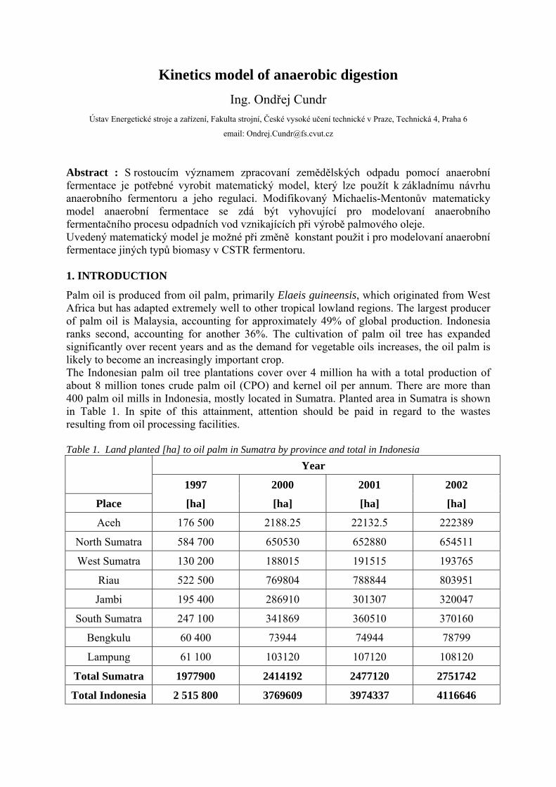
Palm oil is produced from oil palm, primarily Elaeis guineensis, which originated from West Africa but has adapted extremely well to other tropical lowland regions. The largest producer of palm oil is Malaysia, accounting for approximately 49% of global production. Indonesia ranks second, accounting for another 36%. The cultivation of palm oil tree has expanded significantly over recent years and as the demand for vegetable oils increases, the oil palm is likely to become an increasingly important crop. The Indonesian palm oil tree plantations cover over 4 million ha with a total production of about 8 million tones crude palm oil (CPO) and kernel oil per annum. There are more than 400 palm oil mills in Indonesia, mostly located in Sumatra. Planted area in Sumatra is shown in Table 1. In spite of this attainment, attention should be paid in regard to the wastes resulting from oil processing facilities. Table 1. Land planted [ha] to oil palm in Sumatra by province and total in Indonesia

Year

1997 2000 2001 2002

Place [ha] [ha] [ha] [ha]

Aceh 176 500 2188.25 22132.5 222389

North Sumatra 584 700 650530 652880 654511

West Sumatra 130 200 188015 191515 193765

Riau 522 500 769804 788844 803951

Jambi 195 400 286910 301307 320047

South Sumatra 247 100 341869 360510 370160

Bengkulu 60 400 73944 74944 78799

Lampung 61 100 103120 107120 108120

Total Sumatra 1977900 2414192 2477120 2751742

Total Indonesia 2 515 800 3769609 3974337 4116646

2

1.1 THE PROCESS IN PALM OIL MILL

Typical process in a palm oil mill can be briefly described as follows. The fresh fruit bunches, after being harvested from the plantations, are transported to the mill. Each fresh fruit bunch (FFB) consist of hundreds of fruitlets each containing a nut surrounded by a bright orange pericarp which contains the palm oil. The FFB are unloaded on a ramp and put into containers of 3.5 tons each. Sterilization of FFB is done batchwise in an autoclave of 42 tons of FFB capacity (12 containers) with steam at temperature 140°C for 1-1.5 hour in order to avoid fatty acids production by natural enzymes in the mesocarp. The steam condensate coming out from the sterilizer is one of three sources of liquid effluent. The quantity of this effluent varies from one mill to another, with a minimum of just over 0.12 ton for each ton of FFB. The containers with the sterilized bunches are emptied into a rotary drum thresher where the fruits are separated from the bunch stalk. This processing step generates the empty fruit bunches (EFB) at 230-250 kg per ton of FFB. The separated fruits are carried into digesters and mechanically treated into mash. No residue occurs in this step. The oily mash is fed into a continuous screw press system. The extracted oil phase is collected and discharged to the purification section. The remained press cake is transported to a separation system consisting of air classifiers and cyclones for drying and separation of nuts and fibres. Kernels recovered from nuts in crackers are usually transported to kernel oil mill where a screw press extracts kernel oil. Fibres and shells are solid residues obtained during the oil extraction, with the amount of 145 and 60 kg per ton of FFB, respectively. To improve oil clarification, hot water is added to the raw oil and the mixture is passed through a vibrating screen to separate large size solids. The oil, after sieving, still contains small size solids and water. The conventional procedure to separate oil from water and suspended solids is the settling tank method, where the system is heated by steam. The oil that floating on the top is collected by a funnel then sent to a crude oil tank. The settling tank underflow is collected in the sludge tank and subsequently treated to recover the oil. In order to protect the equipment in the subsequent process steps against clogging, the bottom sludge is pre-cleaned by means of microstainer/hydrocyclone of desander. The desanders are cleaned by discharging the accumulated solids to the drain, followed by the injection of fresh water. . The amount of wastewater from this process reaches approximately 0.5 tons per tonne of FFB processed. Total amount of palm oil mill effluent (POME) produced by a single palm oil mill in Indonesia is around 50 tons per hour. See Table 1.1 Table 1.1 Amount of wastewater from typical palm oil mill in Indonesia

Process Quantity [ton] per ton of oil Quantity [ton] per ton of FFB

Sterilizer condensate 0.9 0.12

Clarification sludge 1.5 0.5

Hydrocyclone washing 0.1 0.05

Total 2.5 0.67

3

2. TREATMENT OF PALM OIL MILL EFFLUENT (POME)

The increasingly stringent water quality regulations being introduced in many countries have forced factories to investigate a wide range of approaches for the treatment of palm oil mill effluent (POME) and related wastewaters. These include: simple skimming devices [1, 2]; land disposal [3]; use as animal fodder [4, 5]; ultrafiltration [6, 7]; chemical coagulation and flotation [8, 9, 10, 11]; and various aerobic [12] and anaerobic microbiological processes [14 - 25]. Anaerobic biological digestion systems offer greater potential for the treatment of POME as they do not have such high energy demand of aeration as required by aerobic biological systems [13, 14] and the final product of anaerobic digestion is methane, that can be used to cover energy demands of anaerobic digestion process and palm oil mill process itself. Current method used to solve this problem is anaerobic digestion of POME in open lagoon systems for approximately 120 days in order to reduce biological oxygen demand (BOD) and chemical oxygen demand (COD). Table 1.2 Physical properties of POME [14]

Parameter Range Average Effluent standard *)

pH 3.3 – 4.6 4.1 6 - 9

BOD 8 200 – 35 400 [mg/l] 21 300 [mg/l] 250 [mg/l]

COD 15 100 – 65 000 [mg/l] 35 000 [mg/l] 500 [mg/l]

Total solid 16 600 – 94 100 [mg/l] 46 200 [mg/l] -

Total suspended solid 1 300 – 50 700 [mg/l] 21 200 [mg/l] 300 [mg/l] *) Indonesian National Standard (No. 03/MENKLH/11/1991) 2.1 ANAEROBIC DIGESTION OF POME

The use of conventional anaerobic tank digesters under mesophilic range of temperatures (30-40°C) to treat POME is characterized by long residence times, often it is more than 20 days to achieved chemical oxygen demand (COD) reduction at least 70%. Much better results are reported when two-stage anaerobic digester is used. The first stage is used for acid formation and the second stage is used for methane fermentation. Experiments with conventional anaerobic tank digesters under thermophilic range of temperatures (50-60°C) result in higher than 90% of COD reduction with hydraulic retention time (HRT) above 10 days. Higher biogas yield in thermophilic digestion system compared to mesophilic can be achieved in much shorter time and the concentration of methane in biogas is higher as well. The sulphate reducing bacteria are responsible for the production of H2S in biogas. Their importance in breakdown of organic polymers in anaerobic digestion is not fully understood but they have been shown to be present in anaerobic processing POME. For digesters treating POME at mesophilic temperatures about 105 bacteria can be detected in a ml of anaerobic liquid. In digesters working at thermophilic temperatures only 101 - 102 bacteria were detectable. That represents a reduction of approximately 1000 times in number of these bacteria in the digester. This finding has important implications in the utilization of biogas for

4

generating electricity by the gas engine system or microturbine system where low concentration of the highly corrosive H2S in biogas is desirable. Bearing in mind that the temperature of POME at discharge is between 45 and 60°C, current anaerobic treatment practice using the mesophilic systems requires a lagoon and cooling tower for cooling the wastes. The need of cooling may be eliminated by opting for the thermophilic process. In addition to this, the relatively low heating requirement under tropical conditions makes thermophilic digestion an attractive alternative. In study [25] is shown that in Malaysia with similar temperatures as in Indonesia, the heat requirement is 11% of total heat possible generated by the anaerobic system. The application of modern high rate anaerobic digester technologies such as up-flow or down-flow filters, fluidized beds, up-flow anaerobic sludge blanket (UASB) systems or up-flow floe digesters for the disposal of POME is rare. Some bench-scale experiments have reported COD removal efficiency over 90% in very short hydraulic retention time and high loading rates, but these systems required perfect control system in order to achieve stable conditions in reactor. 3. MATHEMATICAL MODEL FOR ANAEROBIC DIGESTION OF POME

The study of the microbial ecology of the anaerobic digestion process revealed the conversion to be achieved in six different stages after tripping of biogas. They are listed as hydrolysis of biopolymers (proteins, carbohydrates, lipids) into the monomers (aminoacid, sugars and long chain fatty acids), fermentation of amino acids and sugars, anaerobic oxidation of long chain fatty acids and alcohols, anaerobic oxidation of intermediary products such as volatile fatty acids, conversion of acetate to methane and conversion of hydrogen to methane. Several mathematical models to characterize the anaerobic digestion process have been developed. Mathematical models have been proposed simulating paths of conversions. The six steps mentioned above have been further expanded to fourteen steps identifying the decay of five distinct microbial groups, and incorporating protolysis of biocarbonate and deprotolysis of carbone dioxide [27]. In recent years more and more complex mathematical models of anaerobic digestion have been introduced involving many biochemical processes. Yet, due to scarcity of measured data, it is almost impossible to obtain reliable estimates of unknown dynamical parameters. Therefore either simpler, manageable models are needed or data acquisition has to be improved which is difficult especially for microorganisms. In this work the Michaelis-Menten model is adopted for the kinetic studies of the anaerobic digestion. The model can be represented as dS Xdt

µ= ⋅

The limitations of applying this model are:

1. The substrate should be soluble 2. The concentration of metabolic end products should be dilute enough to prevent toxic

or retarding effects on metabolic activity 3. The required nutrients must be maintained in excess so that the organic substrate will

be growth limiting

In anaerobic digestion of POME, limitations 1 and 2 are broadly satisfied. The substrate for methane formation, usually rate determining in anaerobic digestion, is organic acids, which are soluble in water. Limitation 2 is also satisfied because the metabolic end products of

5

anaerobic digestion are mainly methane, carbon dioxide and other gases which are all evolved to atmosphere or gas storage tank. As for limitation 3, the experimental data used for evaluating the kinetics parameters were taken at lower retention time when an abundant supply of substrate is available. Mass balance equations for microorganism in continuous flow system without recycle (continuously stirred tank reactor) can be estimated by equating accumulation against the increases and decreases occurring in an infinitely short time intervals as follows: Rate of accumulation Rate of flow of Rate of flow of Net growth of of microorganism within = microorganism - microorganism + microorganism the system boundary into the system out of the system within the system

boundary boundary boundary This can be written as: accumulation = inflow – outflow + net growth

0dX V q X q X X Vdt

µ⎛ ⎞ ⋅ = ⋅ − ⋅ + ⋅ ⋅⎜ ⎟⎝ ⎠

[1]

Similarly mass balance for substrate (POME) can be expressed as:

0dS V q S q S X Y V m X Vdt

µ⎛ ⎞ ⋅ = ⋅ − ⋅ + ⋅ ⋅ ⋅ + ⋅ ⋅⎜ ⎟⎝ ⎠

[2]

The biomass growth rate µ with Monod kinetic equations may be expressed as in equation [3] and this equation can be further refined by the introduction of decay coefficient Kd due to endogenous respiration as shown in equation [4]

max

s

SK Sµµ ⋅

=+

[3]

max

s

S Kd XK Sµµ ⋅

= − ⋅+

[4]

At steady state condition, there is no accumulation (dX/dt = 0) and concentration of microorganism in the influent can be neglecting, the equation [1] combined with equation [4] reduces to

max Y Sq KdV Ks S

µ ⋅ ⋅= −

+ [5]

The corresponding substrate balance equation, at steady state conditions

max0( ) X SS S Y m x

Ks Sµ ⋅ ⋅

− ⋅Θ = ⋅ − ⋅+

[6]

From the above equations, amount of microorganism and substrate concentration in digester under steady state conditions can be expressed as

6

0S SX

Y m HRT−

=+ ⋅

[7]

max

KsSµ

⋅Θ=

−Θ [8]

The minimum critical hydraulic retention time (HRTc) can be estimated from equation [5]. At minimum critical HRT, S So. Thus, rewriting equation [5] gives

max 0

0

1

s

SY KdHRTc K S

µ ⋅= ⋅ −

+ [9]

The COD reduction efficiency is given by

0

0

100%S SES−

= ⋅ [10]

4. RESULTS AND DISCUSION

Parameters used for simulation were determined from laboratory bench scale experiments of anaerobic treatment of POME under mesophilic conditions at 30°C. All the values of the kinetic constants, Ks, µmax, Y and Kd shown in table 3 are reasonable in view of the high concentration of feed sludge used. Comparable values were also reported by [28], Ks reported values are 5 560 – 13 000 mg/l of COD, for µmax 0.37 – 1.07 mg COD/mg X/day, for Y 0.1 – 0.2 mg X/mg COD and Kd 0.02 1/day. . Comparison of simulated data with experimental data show that Michaelis-Menten kinetic model can be used for anaerobic digestion of palm oil mill effluent in completely stirred tank reactor (CSTR) with continuous feeding. This model could be used for simulation of anaerobic digestion with different types of biomass, when kinetics constants Ks, Y, µmax and Kd are evaluated from experiments. Kinetics parameters in this work were determined only for anaerobic digestion of POME under mesophilic conditions, kinetic parameters for anaerobic digestion of POME under thermophilic conditions will be determined in future work when more relevant data from bench scale digesters will be achievable Table 3. Value of evaluated parameters Ks [mg /l of COD] µmax [mg COD/mg X/day] Y [mg X/mg COD] Kd [1/day] 14 500 0.717 0.193 0.0531

7

Figure 3.1. Comparison of simulated and measured data for substrate concentration in digester

0

1000

2000

3000

4000

5000

6000

7000

8000

9000

0 5 10 15 20 25 30 35

HRT [day]

S [m

g/l]

Figure 3.2. Removal efficiency of COD

0

20

40

60

80

100

120

0 10 20 30 40 50 60

HRT [day]

E[%

]

8

Figure 3.3. Performance of anaerobic digestion of POME at 30°C

0

10000

20000

30000

40000

50000

60000

70000

0 5 10 15 20 25 30 35 40 45 50

HRT[day]

S[m

g C

OD

/l]

NOMENCLATURE

So [mg/l] - substrate concentration in digester feed S [mg/l] - substrate concentration in digester discharge Xo [mg/l] - concentration of microorganism in digester feed X - [mg/l] concentration of microorganism in digester µ [mg COD/mg X/day] - specific growth rate µmax [mg COD/mg X/day] - maximum specific growth rate Ks [mg /l of COD] - half velocity constant Y [mg X/mg COD] - yield coefficient Kd [1/day] - endogenous decay rate constant HRT [day] - hydraulic retention time (HRT=q/V) Θ [1/day] - dilute velocity (Θ=1/HRT) E [%] - COD reduction efficiency m [mg COD/mg X/day] – inhibition coefficient

9

REFERENCES

1. W. Roge and A. Velayuthan, (1981). “Preliminary trials with Westfalia-3-phase decanters for palm oil separation.” In: Push-parajah, E. and Rajadurai, M. (Eds.), Palm Oil Prod. Technol. Eighties, Rep. Proc. Int. Conf., Inc. Sot. Plant. Kuala Lumpur, Malaysia. 327-334. 2. W.J. Ng, A.C.C. Goh and J.H. Tay, (1988). “Palm oil mill effluent treatment - liquid-solid separation with dissolved air flotation.” Biol. Wastes 25, 257-268. 3. A. N. Ma and A.S.H. Ong (1986). “Palm oil processing – new development in effluent treatment.” Water Sci. Technol. 18, 35-40 4. J. Sutanto, (1983). “Solvent extraction process to achieve zero-effluent and to produce quality animal feed from mill sludge.” Planter 59, 17-35 5. M. Turisin, M. Nor and M. S. Suwandi (1981). “Membrane process in by-product recovery.” Sains Malays. 10, 161-174 6. M.A. Badri, (1984).“Identification of heavy metal toxicity levels in solid wastes by chemical specification.” Conserv. Recycl. 7, 257-269. 7. C.C. Ho and C.Y. Chan, (1986). “The application of lead dioxidecoated titanium anode in the electroflotation of palm oil mill effluent.” Water Res. 20, 1523- 1527. 8. K.K. Chin, W.J. Ng, A.N. Ma and K.K. Wong, (1987). “Treatabihty studies of palm oil refinery wastewaters.” Water Sci. Technol. 19, 23-29. 9. M.I.A. Karim, and L.L. Hie, (1987). “The use of coagulating and polymeric flocculating agents in the treatment of palm oil mill effluent (POME).” Biol. Wastes 22, 209-218. 10. K.Abdul, 1. Mohamed and A.Q.A. Kamil, (1989). “Biological treatment of palm oil mill effluent using Trichodermu uiridr.” Biol. Wastes 27, 143-152. 11. J.O. Edewor. (1986). “A comparison of treatment methods for palm oil mill effluent (POME) wastes.” J. Chem. Technol. Biotechnol. 36, 212-218. 12. W.J. Ng, K.K. Chin and K.K. Wong, (1987). “Energy yields from anaerobic digestion of palm oil mill effluent.” Biol. Wastes 19, 257-266. 13. M.S. Suwandi (1981). “Retention characteristic of polyamide and polysulfone membranes in relation to palm oil mill efflunet.” Sains Malays. 10, 147-160 14. T. Setiadi, H. and A. Djajadiningrat (1996). “Palm oil mill effluent treatment by anaerobic baffled reactors: recycle effects and biokinetic parameters.” Wat. Sci Tech. 11, 59-66 15. R. Borja, Ch. J. Banks (1994). “Treatment of palm oil mill effluent by Upflow anaerobic fitration.” J. Chem. Biotechnology, 11, 103-109 16. J. O. Edewor (1996). “A comparison of treatment methods for palm oil mill effluent (POME) wastes.” J. Chem. Biotechnology, 36, 212-218

10

17. A. Ibrahim, B. G. Yeoh, S. C. Cheah, A. N. Ma, S. Ahmad, T. Y. Chew, R. Raj, M. J. A. Wahid (1984). “Thermophilic anaerobic digestion of palm oil mill effluent.” Wat. Sci Tech. 17, 155-166 18. S. Mustapha, B. Ashhuby, M. Rashid, I. Azni (2003). ”Star-up strategy of a thermophilic upflow anaerobic filter for treating palm oil mill effluent.” Trans IchemE 81 part B 19. W. J. Ng, K. K. Chin& K. K. Wong (1987). “Energy Yields from Anaerobic Digestion of Palm Oil Mill Effluent.” Biological Wastes 19 ,257-266 20. R. Borja, Charles J. Banks, B. Khalfaoui, A. Martin (1996). “Performance evaluation of an anaerobic hybrid digester treating palm oil mill effluent.” J. Environ. Sci. Healt A31, 1379-1393 21. R. Borja, Ch. J. Banks, E. Sinchez (I 996). “Anaerobic treatment of palm oil mill effluent in a two-stage up-flow anaerobic sludge blanket (UASB) system.” Journal of Biotechnology 45, I25- 135 22. K. K. Chin, K. K. Wong (1983). “Thermophilic anaerobic digestion of palm oil mill effluent.” Water Res. 17. 993-995 23. R. G. Cail, J. P. Barford (1985). “Thermophilic semi-continuous anaerobic digestion of palm oil mill effluent.” Agricultural wastes 13, 295-304 24. C. C. Ho, Y. K. Tan (1985). “Anaerobic treatment of palm oil mill effluent by tank digesters.” J. Chem. Tech. Biotechnology 35B, 155-164 25. T. O. Peyton, I. W. Cooper (1979). “Mesophilic and thermophilic anaerobic tank treatment of palm oil mill wastewaters.” Proceedings of the industrial waste conference 34th. 26. K.O. LIM (1998). “Oil Palm plantations – A plausible renewable source of energy.” International Energy Journal 20 27. H. Siegrit, D. Renggli, W. Gager (1993). “Mathematical modelling of anaerobic mesophilic sewage sludge treatment.“ Wat. Sci. Tech. 27(2), 25-36

MEASURING OF FLOW FIELDS INSIDE CYLINDER OF

ONE-CYLINDER SPINNING ENGINE MODEL USING PIV

Ing. Miloslav Emrich1

SHRNUTÍ

Příspěvek popisuje zařízení určené k měření proudových polí ve válci protáčeného modelu spalovacího motoru užitím rovinné laserové anemometrie (PIV). Zařízení je složeno z jednoválce poháněného elektromotorem, měřícího válce s optickým přístupem pro laserový list a kamery, hlavy z motoru Škoda 1,2 HTP a PIV aparatury firmy Dantec. Optický přístup pro kamery do válce je řešen užitím endoskopů. Ukázka výsledků z prvního měření je také součástí příspěvku.

Klíčová slova: PIV, proudové pole, válec, motor, endoskop, částice

ABSTRACT

This article describes experimental test bed for measuring of flow fields inside the cylinder using particle image velocimetry (PIV). The setup consists of single-cylinder engine drived by electric motor, engine cylinder with optical access for laser light, camera equipment, cylinder head (Skoda 1.2 HTP) and PIV system from Dantec. The optical access for digital camera is accomplished through the endoscope optics. Some results from first measurements are presented here. Key words: PIV, flow field, cylinder, engine, endoscope, particles

1. INTRODUCTION

Main aim of every engine engineer dealing with inside cylinder aerodynamics is to ensure the fuel evaporation and proper mixing of fuel with air in order to achieve homogenous mixture. Flow fields and turbulence influence this task considerably. Moreover, the stability of flow field, especially of its vortex formation during the compression stroke provides fast combustion resulting in improved engine power, fuel consumption and some emissions.

An idea of measuring of incylinder flow fields within one-cylinder spinning engine model (Figure 1.1) using particle image velocimetry (PIV) was performed on the basis of the experiences with measuring flow fields in aerodynamic air track using PIV - see [1] and [2].

This new set-up called „AEROMODEL“ presented in this paper should provide more detailed sight into the combustion chamber and be compared to previous model arrangement 1 Ing. Miloslav Emrich; Czech Technical University in Prague; Faculty of Mechanical Engineering; Department of Automotive, Railway and Aerospace Engineering; Technická 4, 166 07 Praha 6; tel. +420 22435 2496; e-mail : miloslav.emrich@fs.cvut.cz

without piston and moving valves. Therefore measuring of flow fields inside cylinder during intake and compression stroke is now possible and gives results which are close to real engine operation.

Figure 1.1 Test bed with particles box in the front

2. TEST BED DESCRIPTION

The Aeromodel test bed (Figure 2.1) - was made by reconstructing of old arrangement, which had had similar utilization. The Aeromodel is one-cylinder spinning model engine with adjustable compression ratio and stroke. This is done by adjustable length of connecting rod (from 180 to 280mm) and connecting rod pin radius (from 32 to 75mm). The crank-shaft is powered by electromotor with peak power of 3 kW at 2860 rpm and regulated by a frequency converter. The electromotor drives a rotating fly-wheel (mass of 105kg, moment of inertia of 4,22 kg.m2). Whole crank mechanism is connected through the electromagnetic switch clutch with the fly-wheel equipped with band-break. The maximum fly-wheel speed is 1000 rpm. Overhead camshaft is moved by chain that is strained by a stretcher.

Skoda 1.2 HTP engine cylinder head is used. This head has two valves for each cylinder. Special piston and measuring cylinder with optical access for digital camera inside the cylinder through the endoscope is used (Figure 2.2 and Figure 2.3).

Figure 2.1 State of art Aeromodel Figure 2.2 Engine cylinder, endoscope and engine head with timing chain

A special construction of piston is used because of the impossibility of lubricating

cylinder wall. The piston consists of two iron desks holding carbonaceous-silon sealing ring (Figure 2.3), that is self lubricating.

The usage of PIV method requires optical access for laser sheet and camera into the cylinder. Optical access for laser sheet is made by milling two vanes in opposite side of cylinder. These vanes go into the cylinder through glass sheets made from BK7 which are fixed on the cylinder by metal desks. Sealing tape is used for sealing.

Optical access for camera is made through endoscope Karl Storz (diameter 8mm) with top angle 67° (Figure 2.2). Five holes with threads were made in the cylinder. The endoscope goes inside the cylinder through these holes. The position of these holes was designed to see whole area of cylinder about 50mm below cylinder head (Figure 2.4).

The measuring of flow fields in various planes going through the axis of cylinder are possible. The change of measuring plane could be done by angular rotation of cylinder.

The revolutions of fly-wheel and crank mechanism are shown on a sectional counter. A signal level (TTL) for the sectional counter is also used for synchronization of laser sheet. TTL impulses are initialized by a circular desk with one slot and optical gate. When the light from emitter goes through the circular desk, TTL signal is started up. The right moment for laser sheet to switch on is set by the angular position of circular desk slot to TDC.

The marking particles inside the cylinder are necessary for visualization of the flow fields. They are stored in a container (750x750x270mm). A fan inside, mixes particles with

air (Figure 1.1). The mixture of particles and air is sucked into the cylinder and returned back to the container through flexible pipes.

Figure 2.3 Model of test cylinder and piston (Catia V5)

Figure 2.4 Cylinder section: Model with laser sheet (green) and position of endoscope with visible area (yellow circles) (Catia V5)

3. RESULTS

The first measurement was performed to check functionality of the Aeromodel at 400 RPM. The Expancel particles (diameter 100μm) were used for this measurement. These particles were not suitable because they were agglomerated to larger pieces. Therefore the Dantec particles (diameter 5μm) were further used. They are made of polyamide and they are designed for use in water.

The flow fields were measured in position of 110° after TDC during intake stroke. It was tested in four possible endoscope positions.

About 100 double-frames were always made in each position of the endoscope. Endoscope optics deforms pictures – fish eye effect. Before evaluating the pictures, it is necessary to transform deformed pictures into the plane. The scale of picture is set by the calibrating target. This target is also used to transform pictures into the plane. A calibrating target and pictures of open valve before and after transformation, are shown in Figure 3.1 and Figure 3.2. There are also some undesirable reflections of laser sheet on valve and bellow the valve. White dots are the laser illuminated marking particles.

250 300 350 400 450 500 550 600 650 700 750 800 850 900 950 1000 1050 1100 1150 1200 1250 1

250

300

350

400

450

500

550

600

650

700

750

800

850

900

950

1000

pix

Image size: 992×900 (260,124), 12-bitsBurst#; rec#: 9; 1 (9), Date: 22.6.2005, Time: 18:57:20:746Analog inputs: 1 763; 1 758; 1 758; 1 768

250 300 350 400 450 500 550 600 650 700 750 800 850 900 950 1000 1050 1100 1150 1200 1250

250

300

350

400

450

500

550

600

650

700

750

800

850

900

950

1000

pix

Image size: 992×900 (260,124), 12-bits (frame 1)

Burst#; rec#: 1; 1 (1), Date: 23.6.2005, Time: 21:05:50:750

Figure 3.1 A picture before transformation: The calibrating target and a valve view through the top left endoscope into the cylinder

-15 -10 -5 0 5 10 15 20 25 30mm-25

-20

-15

-10

-5

0

5

10

15

mm

Image size: 120.0×97.5 mm (-50.0,-47.5), in pixels: 2111×1715, 12-bitsBurst#; rec#: 9; 1 (9), Date: 22.6.2005, Time: 18:57:20:746Analog inputs: 1 763; 1 758; 1 758; 1 768

-15 -10 -5 0 5 10 15 20 25 30 35mm25

-20

-15

-10

-5

0

5

10

15

mm

Image size: 120.0×97.5 mm (-50.0,-47.5), in pixels: 2111×1715, 12-bits (frame 2)Burst#; rec#: 1; 1 (1), Date: 23.6.2005, Time: 21:05:50:750Analog inputs: 1 763; 1 763; 1 777; 1 768

Figure 3.2 A picture after transformation

A description of evaluation procedure using software FlowManager ver.4.5: • Cross-correlation analyze, the evaluation area 32x32 pixels, overlap 25% • Peak Validation – 1,2 • Moving Average – area 5x5 pixels, acceptable factor 0,1 • Filtering - area 3x3 pixels

This process of evaluation was applied to all measured double-frames. It was calculated to obtain statistically average picture of flow field for each position of endoscope in the cylinder. An example of measured flow field is presented in Figure 3.3. The vortexes are highlighted by blue dashed line. The areas where it was impossible to calculate the flow field are marked by red crosshatch areas. Already mentioned light reflection were situated in these areas .

-15 -10 -5 0 5 10 15 20 25mm-25

-20

-15

-10

-5

0

5

10

mm

Statistics vector map: Vector Statistics, 33×30 vectors (990)Size: 454×413 (-133,-230)

Top-left – opened intake valve

25 -20 -15 -10 -5 0 5 10 15 20 mm20

-15

-10

-5

0

5

10

15

20

25

mm

Vector map: Filtered, 29×29 vectors (841), 841 substitutedBurst#; rec#: 1; 1 (1), Date: 23.6.2005, Time: 21:58:54:077Analog inputs: 1.763; 1.759; 1.763; 1.768

Top right – exhaust valve

-25 -20 -15 -10 -5 0 5 10 15 20mm-20

-15

-10

-5

0

5

10

15

mm

Statistics vector map: Vector Statistics, 17×14 vectors (238)Size: 456×377 (-247,-187)

Bottom-left - piston

5 -20 -15 -10 -5 0 5 10mm

-20

-15

-10

-5

0

5

10

15

20

mm

Statistics vector map: Vector Statistics, 20×24 vectors (480)Size: 348×417 (-213,-216)

Bottom-right - piston

Figure 3.3 Velocity vectors obtained from the measurement

There is a picture of opened intake valve in the Figure 3.3 (top-left). A global flow field in this part is orientated to the cylinder head. There is a significant vortex formation below intake valve. This vortex is formed along intake flow nearby cylinder wall.

Figure 3.3 (top-right) presents closed exhaust valve. Evident continuous inflow and nook swirl is situated under the exhaust valve.

Figure 3.3 (bottom-left) presents flow field influenced by the piston in the top direction. Figure 3.3 (bottom-right) shows continues inflow. When the flow comes into the piston it starts to return to the cylinder head. This flow forms vortex.

4. CONCLUSION

This paper has presented unique test bed for measuring of flow fields inside the cylinder.

It is necessary to notify that flow fields measured using PIV method show only velocity component within the laser sheet plane. This plane goes through axis of the cylinder. It is common that vortex (swirl) with the same axis as cylinder, appears when using two-valve cylinder head. However, this vortex inside the cylinder may have a great tangential velocity component, which is impossible to measure in only one plane. There are some possible solutions to cope with this problem: to measure the flow fields in many planes, that go through the axis of the cylinder and to calculate velocity component using equation of continuity in cylindrical coordinates; using Stereo-PIV measurement; to measure in plane perpendicular to the cylinder axis using glass cylinder. In the next step these solutions will be evaluated and one of these selected for future measurement.

Another disadvantage of our first measurement is the impossibility of joining flow fields from various endoscope positions. This fault will be solved using collective calibrating target see Figure 3.1.

For next measurement the old particles, originally intended for water measurements, will be replaced with new type of particles that are acceptable for our air measurements - EXPANCEL® MICROSPHERES 461 DET 40 d25 with diameter range from 35 to 55 μm and density 25±3 kg.m-3.

From this first measurement using above described unique Aeromodel test bed follows: This PIV method with the usage of endoscope optics seems to be a fairly good and precise for measurement of flow fields inside the cylinder of the engine. The testing of various types of cylinder heads will continue and the results will be compared with simulation and presented in author’s doctoral thesis.

5. LITERATURE

[1] Hatschbach, P.: Measurement in Model of Internal Combustion Cylinder at Steady Flow Condition using PIV, In: 18th Symposium on Anemometry, Prague, Institute of Hydrodynamics, 2003, Part 1, Page 33-36. ISBN 80-239-0644-5

[2] Hatschbach, P. - Novotný, J.: Endoscopic PIV Measurements in Cylinder of IC Engines, In: Colloquium Fluid Dynamics 2003. Prague: Institute of Thermomechanics, Academy of Sciences of the CR, 2003, Part 1, Page 25-26. ISBN 80-85918-83-8.

[3] Emrich, M.: Description of set-up for measurement flow fields inside cylinder of combustion engine model using PIV. In: 19th Symposium on Anemometry. Prague: Institute of Hydrodynamics ASCR, 2005, Part 1, Page. 35-36. ISBN 80-239-4871-7.

ACKNOWLEDGMENT

Improvement of Aeromodel was made thanks to internal grant Czech technical university, Faculty of Mechanical Engineering, 2004.

Workplace and additional improvements were done thanks to grant FRVŠ NO.131/2005.

PIV device is supported by Josef Božek research center of Engine and Automotive Engineering - 1M0568, MŠMT Czech republic

České vysoké učení technické v Praze

Fakulta strojní

Ústav procesní a zpracovatelské techniky

Stochastic approach to describe population dynamics of yeast

Candida utilis during fermentation process.

Ing. Jakub Horák

2

Abstrakt Tato práce se zabývá simulací vývoje distribuční funkce kvasinkových buněčných kultur stochastickým přístupem. Měnící se populační bilance mikrobiálních kultur je popsána systémem parciálních integro-diferenciálních rovnic (deterministický přístup), jejichž řešení je proveditelné jen pro jednoduché případy. Kvasinky nevyhovují podmínce binárního dělení (mateřská buňka se rozdělí na dvě stejné dceřinné buňky), ale dělí se pučením (malý pupen, velká mateřská buňka). Byl vyvinut stochastický model zahrnující růst, úmrtí a dělení buněk pučením. K získání evoluce distribuční křivky kvasinek podle jejich velikosti je užito Markovových řetězců. Výstupy jsou fitovány na naměřený vývoj distribuční křivky kvasinky Candida utilis a zhodnoceny. Abstract This paper is concerned with the simulation of evolution of distribution function of yeasts microbial culture with stochastic approach. Population balance of microbial cultures is formulated as deterministic process by system of partial-integro-diferencial equations whose solution is still performable for the simplest cases. Yeast culture does not satisfy a condition of binar fission (mother cell splits into two equal doughter cells), but new offsprings originate from spring up process (mother cell splits into two inequal doughter cells). Stochastic numerical model captured growth, death and split of cells is developed. To get evolution of distribution of yeasts according its size is used continuos-time finite-state Markovian chains. Outcomes are fitted to measured evolution of distribution of yeasts Candida utilis with laser particle counter and discussed. 1. Introduction Population dynamics are concerned with the evolution of some properties of a population with time, and its dependence on the initial and environmental conditions. In this paper is illustrated how Markov chains can be used as the basis for modeling and simulating population dynamics of yeasts. Markov chain is well-known subject introduced by Markov in 1906. Stochastic models and Markovian terms can be applied for any real-world systems under some uncertainty. Once Markovian model is established, it can be used to describe the behavior of the system, or more significantly to deeply explore its dynamics. It follows the solution of the so-called forward equations which provides the evolution of the probability distribution. This distribution of probability is obtained from Markov chains, which are based on the specification of the generator and the initial conditions.

3

2. Markovian chains and Chapman-Kolmogorov equation Stochastic process is a collection of random variables ( ) tα defined on a common probability space and indexed by the time parameter t. For a fixed t α is a random variable. The state space of ( )tα is the collection of all values it may take. Markov chain is stochastic process which satisfies the so-called Markov property – for which given the current state, the probability of chain’s future states is not affected by any knowledge about its states in past. When transition probabilities (probability of moving between possible states) does not change in time the Markov chain is called time-homogeneous or stationary:

( ) ( ) ( ) 0 ≥==+= sallforisjstPtPij αα (1.) and relevant transition matrix is in finite-state space i=<1,m>:

( )

( ) ( ) ( ) ( )( ) ( ) ( ) ( )

( ) ( ) ( ) ( )

=

−

−

−

tPtPtPtP

tPtPtPtPtPtPtPtP

tP

mmmmmm

mm

mm

,1,2,1,

,21,22,21,2

,11,12,11,1

L

MMOMM

L

L

(2.)

For each Markov chain ( ) ∑=

=≥m

jijij PtP

1

1,0 holds Chapman – Kolmogorov equation:

( ) ( ) ( )∑=

=+m

kkjikij hPtPhtP

0 (3.)

It means, to move from state i to state j in time interval (t+h), Markov chain moves to some state k between states i and j. And in the remaining time Markov chain moves from state k to state j. Moreover:

( ) ( )ijtqQ

tItP

==−

+→0lim (4.)

I - identity matrix Q - infinitesimal generator (represents rates of change of the transitions) It satisfies the differencial equation:

( ) ( ) ( ) IPQtPdt

tdP== 0 (5.)

4

And probability distribution of the Markov chain during time is:

( ) ( ) ( ) 00 ppQtpdt

tdp== (6.)

p0 - initial distribution It has a solution:

( ) ( )Qtptp exp0= (7.) And mean moment can be computed by:

( ) ( )∑=

=m

ii tiptE

1α (8.)

( )tEα - total number of particles

pi(t) - i-th component of p(t) To describe such system is necessary to define infinitesimal generator Q. 3. Formulation yeasts population dynamics during fermentation process To assemble a stochastic model for growth, split and death process of yeast fermentation it is necessary to make some assumptions:

(1) The population is well mixed – each yeast acts independently (2) The yeasts of a population differ in size and individual yeasts of different sizes heve

different growth, split and death rates. (3) There are sufficient nutrition supplies, i.e. influence of substrate concentration can be

neglected. (4) Growth, split and death rates do not vary in time.

To determine amount of possible states in which yaests can occur is advantageously used outcome from laser particle counter which carried out measures of distribution function. It is division the entire population into k section according to the size of individual yeasts. In addition there is another special state – absorbing state a. The yeasts in division ki ≤<1 may die and enter the a division. All yeasts in division a are dead and can’t grow and split. This is depicted in Fig. 3.1. On Fig. 3.2 is showed how yeasts can move between states in each time interval. Splitting of yeasts by spring up process is simulated as follows: yeast in division

ki ≤≤3 can splits into divisions i-1 and 1. Note that yeasts occur in the same division have the same growth, split and death rates.

5

1 2 3 4 k

a

growth split death

Fig. 3.2. Possible states transition

k-1

1 2 3 k a …..

N

Fig. 3.1. Possible states overview

6

4. Infinitesimal generator Based on assumptions mentioned above is assembled infinitesimal generator:

( )( ) ( )

( ) ( )

( ) ( )( ) ( )

+−−++−−

++−−++−−

+−−

=

−−−−−−−−−

00000000100

100

010001000

0000

111111111

444444444

333333333

2222

11

kkkkkkk

kkkkkkkkk

Q

µγµγξγξµλγµλγξγξ

µλγµλγξγξµλγµλγξγξµλµλ

λλ

LL

L

MMMMMMMM

L

L

LL

LL

λ - growth rate µ - death rate γ - split rate ξ - portionning rate Note that parameters λ, µ, γ and ξ ∈ >< 1,0 and ( ) ( )∑

≠

−=ij

ijii tqtq .

Portionning rate ξ describes amounts of doughter yeasts from splitting mother yeast. 5. Simulation and results Simulation consists of solution of family of ordinary differential equations and making graphic outcomes to compare with measured out data. Determining appropriate λ, µ, γ and ξ is key to understand behavior of fermentation process. It is used Matlab to make all mentioned steps. On figure 5.3 is depicted evolution of distribution function of Candida utilis measured out in Institute of Microbiology the Academy of Sciences of Czech Republic and on figure 5.4 is depicted simulated evolution of this yeast. It is showed that curves are practically identic.

7

Evolution of distribution of yeast Candida utilis

0

5

10

15

20

25

30

1 10 100

[µm]

[%]

1h

2h

3h

Fig. 5.3. Measured distribution function

Fig. 5.4. Computed distribution function

8

6. Conclusions In this paper is showed that stochastic approach using Markov chains can be used for modeling evolution of distribution function during fermentation process. Numerical values of rates λ, µ, γ and ξ must be now resolved to deeply understand when and why there is a change of splitting, dying, etc. By the time rates λ, µ, γ and ξ will be interpreted correctly we gain comprehensive knowledge about fermentation process and interactions in fermentor. Also this is tool with we can get missing information necessary for solving partial integro-differencial equations to describe population dynamics by deterministic approach.

9

References [1] Berovic, M. Bioprocess engineering course. National Institute of Chemistry 1998.

[2] Feller, W. An introduction to probability theory and its applications. Wiley 1957.

[3] Gerstlauer, A., Gahn, C., Zhou, H., Rauls, M.,Schreiber, M. Application of population balances in the

chemical industry - curent status and future needs. Chem. Eng. Sci. 2005. [4] Godin, F.B., Cooper, D.G., Rey, A.D. Development and solution of a cell population balance model

applied to the SCF process. Chem. Eng. Sci. 1999. [5] Godin, F.B., Cooper, D.G., Rey, A.D. Numerical methods for a population-balance model of a

periodic fermentation proces. AIChE Journal 1999. [6] Hounslow, M.J. A discretized population balance for continuous systems at steady state. AIChE

Journal 1990. [7] Marchisio, D.L., Fox, R.O. Solution of population balance equations using the direct quadrature

method of moments. Journal of Aerosol Science 2004. [8] Mitchell, D.A., von Meien, O.F., Krieger, N. A review of recent developments in Modeling of

microbial growth kinetics and intraparticle phenomena in solid-state fermentation. Biochem. Eng. Journ. 2003.

[9] Nielsen, L.K., Reid, S., Greenfield, P.F. Cell size model to describe animal cell size variation and lag

between cell number and biomass dynamics. John Wiley & Sons, Inc. 1997. [10] Nicmanis, M., Hounslow, M.J. Finite-element methods for steady-state population balance

equations. AIChE Journal 1998. [11] Ramakrishna, R., Ramkrishna, D., Konopka, A.E. Microbial growth on substitable substrates:

characterizing the consumer-resource relationship. John Wiley & Sons, Inc. 1997. [12] Ramkrishna, D. Population balances - theory and applications to particulate systems in engineering.

Academic Press 2000. [13] Randolph, A.D., Larson, M.A. Theory of particulate processes. Academic Press 1988.

[14] Rigopoulos, S., Jones, A.G. Finite-element scheme for solution of the dynamic population balance

equation. AIChE Journal 2003. [15] Shi, D., El-Farra, N.H., Li, M., Mhaskar, P., Christofides, P.D. Predictive control of particle size

distribution in particulate processes. Chem. Eng. Sci. 2005. [16] Yin, K. K., Yang, H., Daoutidis, P., Yin, G. G. Simulation of population dynamics using continuous-

time finite-state Markov chains. Computers & Chemical Engineering 2003. [17] Wulkow, M., Gerstlauer, A., Nieken, U. Modeling and simulation of crystallization process using

parsival. Chem. Eng. Sci. 2001.

Description of Lambda-Control Behavior and Exhaust Gas After-

Treatment Ing. Ľubomír Miklánek

Shrnutí

Náplní příspěvku je popis chování jednoprahové lambda regulace a změny v technické účinnosti třícestného katalyzátoru zážehového motoru, provozovaného na zemní plyn. Autor se v článku zaměřil na shrnutí postupů a výsledků experimentálního výzkumu pro vyšetření změn technické účinnosti katalyzátoru vlivem změn parametrů lambda regulace.

Abstract

Description of lambda-control behavior is a content of the article together with a description of changes in technical efficiency of three-way catalyst. Lambda-control loop and exhaust gas after-treatment using three-way catalyst are accessories of natural gas-fuelled spark-ignition engine. Focus is laid on the results from experimental investigation of changes of three-way catalyst technical efficiency, which are depended on changes of lambda-control loop parameters.

1. Introduction

As part of research and development (R&D) activities on internal combustion engines (ICE) at the ICE laboratory of the Faculty of Mechanical Engineering CTU in Prague, research on various types of natural gas-fuelled spark-ignition engines is performed. These engines are used in co-generation units, usually driving an alternator and also a source of heat. Emission limits for CO (carbon monoxide) and NOx (nitrogen oxides) are very strict for stationary engines, as set out, for example in the TA-Luft regulation. In order to achieve low emissions level, exhaust gas after-treatment is important to reduce all of three monitored pollutants CO, NOx, and HC (hydrocarbons). There are a variety of options for decreasing of these particular pollutants. One of them is application of a so-called three-way catalyst (TWC) as used in conventional gasoline-fuelled engines. In order to achieve good conditions for conversion all of three monitored pollutants in three-way catalyst, it is necessary to keep the mixture strength very close to the so-called stoichiometric value (λ=1). Usually a closed-loop mixture strength control system is used to perform this task. [1], [2]. The molar fraction of CO and NOx in exhaust gas (downstream of the catalyst) is very low as long as the catalyst and the closed-loop mixture strength control system works properly. Usually an emission level is obtainable that is lower than that for a lean-burn engine. During various experiments on ICE equipped with λ-control system, there was observed that conversion efficiency of particular pollutants is changed by change of parameters of λ-control. Just this phenomenon – dependence of efficiency of conversion in three-way catalyst on the setting of λ-control parameters has been investigated. Progress of investigation and obtained results are presented below.

λλ--sseennssoorr

Intake manifold

EExxhhaauusstt mmaanniiffoolldd

λλ--EECCUU

IICC inneennggi ee

Air MMiixxttuurreeEExxhhaauusstt

ggaass

FFuueell--mmeetteerriinngg

GGaass

NNGG ddiissttrriibbuuttiioonn,,

pp==22..11 kkPPaa

ZZeerroo--pprreessssuurree ccoonnttrrooll vvaallvvee

AAccttuuaattoorr

3-way catalyst

TThhrroottttllee

BBaassiicc AAddjjuussttmmeenntt

TD

Dynamometer

Figure 2.1: Layout of the λ-control loop used on the examined engine.

2. Description of the λ-Control System

The conventional layout of a closed-loop λ-control system is illustrated in Figure 2.1. A λ-sensor is installed in the engine exhaust manifold upstream of the catalyst. The sensor generates a voltage, which depends on the exhaust gas oxygen content. Its response is very steep when mixture strength lies within the narrow range of air-excess value near λ=1.

The moveable part of the fuel-metering orifice is usually driven by a step motor (actuator). A so-called one-threshold λ-control system is used for investigation. This type of λ-control system is not the best for transient engine regimes but it is suitable for mentioned research due its simplicity. In case of this type of λ-control system, the actuator moves with constant velocity independently of value of λ-sensor voltage output.

The λ-electronic control unit (λ-ECU) transmits (with constant frequency) pulses for the step motor to increase/decrease the cross section area of the fuel-metering orifice as the actual λ-sensor voltage output becomes lower/higher than the preset threshold voltage.

During operation of the engine there is a transportation delay between the mixer and the λ-sensor. That’s why a change of fuel flow at the inlet port of the mixer is detected using λ-sensor in exhaust manifold with time delay. This delay is represented in Figure 2.1 by the parameter TD. This delay decreases as the flow of working fluid through the engine increases and vice versa.

The threshold voltage (Uset) and basic step frequencies (by parameter Sfrq) are electrically adjustable. Moreover, the intensity of mixture strength response to actuator movement is influenced by the position of a manually adjusted screw, which is usually

installed in the fuel pipeline upstream of the fuel inlet port of the mixer. This screw is marked in Figure 2.1 as Basic Adjustment. Therefore, there are total of three adjustable elements available for optimization of system behavior.

3. Description of Way of Work of λ-Control System

Way of work of one-threshold λ-control loop is illustrated in Figure 3.1. Course of λ-sensor voltage output is represented by a dashed line, course of steps of actuator is represented by a solid line. The areas of rich (λ<1) and lean (λ>1) mixture are defined by parameter threshold voltage (Uset). In this example a standard so-called jump-characteristic of used λ-sensor is assumed. In Figure 3.1 the rich mixture is assumed at the beginning. Thus, λ-ECU is closing fuel-metering orifice by actuator till λ-sensor voltage output crosses the value of threshold voltage. This means, mixture become lean. A phase, in which the λ-sensor voltage output is higher than threshold voltage, is so-called Rich phase, marked as RP. Because the mixture is lean, λ-ECU is opening the fuel-metering orifice by actuator till λ-sensor voltage output crosses the threshold voltage. This means, mixture become rich. A phase, in which the λ-sensor voltage output is lower than threshold voltage, is so-called Lean phase, marked as LP. As it has been already mentioned, there is the transportation delay between mixer and λ-sensor. That’s why the change of mixture does not occur immediately, as we can see in Figure 3.1. Sfrq (time delay) is next parameter, see Figure 3.1. This parameter means time delay between consecutive steps of step motor (actuator).

TTiimmee [[ss]]

UU [[VV]]

UUsseett

RRPP LLPP

Fuel-metering orifice

SSffrrqq

SStteeppss [[--]]

LLPP

RRPP λλ >> 11

λλ << 11

SSffrrqq –– TTiimmee ddeellaayy [[ss]]

UUsseett –– TThhrreesshhoolldd vvoollttaaggee [[VV]]

RRPP –– RRiicchh PPhhaassee LLPP –– LLeeaann PPhhaassee

Figure 3.1: Way of work of the one-threshold λ-control loop. Both of parameters Uset [V] and Sfrq [s] are so-called parameters of λ-control. Parameter Sfrq is adjustable only by appropriate software via serial port RS 232 of computer. Parameter Uset is adjustable by potentiometer that is a part of the λ-ECU.

During experimental investigation on ICE equipped with one-threshold λ-control loop there was observed that:

parameter Uset influences a steady-state value of λ, parameter Sfrq influences amplitudes of λ in rich and lean phases and slightly a steady-

state value of λ as well.

4. Mathematical model of λ-control loop

To ensure the high effectiveness of the development procedure, a mathematical model of λ-control system behavior [3] has been created in author’s laboratory using TestPoint [4] development environment. This mathematical model is still further improved. To obtain better results in simulation of work of λ-control loop in transient regimes of engine, the modification of this model was created. Results from this modified mathematical model were experimental verified and they were published in [5]. The interactive panel of modified mathematical model of λ-control loop is shown in Figure 4.1. To make this paper more complete, mathematical model of λ-control behavior is mentioned here, although it is not a content of the article. Detailed description of this model is presented in [5].

Figure 4.1: The interactive panel of the modified mathematical model of λ-control loop.

5. Observed Phenomenon in Conversion – Ground for This Topic

During experimental investigation on λ-control loop a dependence between conversion rate of particular pollutants in catalyst and setting of parameters of λ-control has been observed. Mentioned phenomenon is presented in Figures 5.1 and 5.2. In these figures measured molar fractions of CO, NOx and HC are shown. These data were measured in steady-state engine operation: 3000 RPM, at W.O.T., Uset = 0.77 V. Values of Sfrq were chosen: 252, 200, 152, 100, 52 and 32 ms. Values of Sfrq are depicted in Figures 5.1 and 5.2.

In Figure 5.1 the molar fractions measured upstream of catalyst are shown, whereas in Figure 5.2 the molar fractions measured downstream of catalyst. Molar fractions of pollutants were measured using laboratory set of analyzers, in dry exhaust gas.

252 200 152 100 52 32

HC [ppm]NOx [ppm]

CO [ppm]0

1000

2000

3000

4000

5000

6000

Sfrq [ms]

HC [ppm]

NOx [ppm]

CO [ppm]

Figure 5.1: Molar fractions of pollutants measured upstream of catalyst.

In Figure 5.1 it is clearly visible, that setting of parameter Sfrq influences pollutants levels upstream of catalyst only slightly.

Another situation is downstream of catalyst. In Figure 5.2 it is visible, that setting of Sfrq influences pollutants levels considerably. And just description of circumstances that activate this phenomenon is ground for this topic.

252 200 152 100 52 32

NOx [ppm]CO [ppm]

HC [ppm]0

50

100

150

200

250

300

350

400

450

500

Sfrq [ms]

NOx [ppm]

CO [ppm]

HC [ppm]

Figure 5.2: Molar fractions of pollutants measured downstream of catalyst.

6. Investigation of Phenomenon by Experimental Way

Research has been carried out by combination of experimental way and mathematical simulation on the base of measured dependences. In order to gain better understanding of the behavior of exhaust gas after-treatment in dependence on setting of parameters of λ-control, it is necessary to perform experiments.

6.1. Equipment for investigation

Equipment for experiments are placed in laboratories of Josef Bozek Research Centre at CTU in Prague. Main equipment for research are:

test bench equipped with a natural gas-fueled engine with one-threshold λ-control loop and three way catalyst (Pt : Rh = 5 : 1),

DAQ system, laboratory set of analyzers,

6.2. Limitation range of investigation

In order to find a range of threshold voltage values in which conversion of each particular pollutant is changed by change of parameter Sfrq, number of experiments has been performed with various value of Uset. Regime of tested engine was: 3000 RPM = const., at W.O.T. Values for Uset were chosen: 0.79, 0.77, 0.75, 0.71, 0.67 and 0.55 V and values of Sfrq were chosen: 252, 200, 152, 100, 52 and 32 ms. Molar fractions of particullar pollutants were measured downstream of catalyst.

As it is visible in Figure 6.1, mixture is too rich in regime at Uset = 0.79 V and conversion rate of CO and HC is low.

252 200 152 100 52 32

NOx [ppm]HC [ppm]

CO [ppm]0

200

400

600

800

1000

1200

1400

1600

1800

2000

Sfrq [ms]

NOx [ppm]

HC [ppm]

CO [ppm]

Figure 6.1: Measured molar fractions of pollutants in regime at Uset = 0.79 V.

On the opposite side, mixture is too lean in regimes with settings of Uset = 0.71 V and less. Conversion rate of NOx is very low, as it is visible in Figure 6.2.

So, range for further investigation was defined by this way (Uset = 0.77 and 0.75 V). Please note, that hydrocarbons (HC) are represented by Methane (CH4) in this article.

Methane has a lower reactivity than other hydrocarbons [2]. That’s why the conversion of HC in catalyst is very difficult, as it is visible in Figures 6.1 and 6.2.

252 200 152 100 52 32

CO [ppm]HC [ppm]

NOx [ppm]0

200

400

600

800

1000

1200

1400

1600

1800

2000

Sfrq [ms]

CO [ppm]

HC [ppm]

NOx [ppm]

Figure 6.2: Measured molar fractions of pollutants in regime at preset Uset = 0.71 V. 7. Evaluation of Measured Data

In limited range as given above, courses of data listed below have been especially investigated:

courses of λ-sensor voltage output (Ulam), courses of steps of actuator, measured steady-state values of particular pollutants downstream of catalyst in

each point of measurements

0

0.1

0.2

0.3

0.4

0.5

0.6

0.7

0.8

0.9

0 10 20 30 40 50Time [s]

Ula

m [V

]

Sfrq= 252 ms Sfrq= 200 ms Sfrq= 152 ms Sfrq= 100 ms Sfrq= 52 ms Sfrq= 32 ms

Figure 7.1: Measured courses of λ-sensor voltage output at preset Uset = 0.75 V.

Measured courses of λ-sensor voltage output are presented in Figure 7.1. These courses were measured at preset parameter Uset = 0.75 V = const. and at various values of parameter Sfrq. It is visible in Figure 7.1, that the shorter is motion period (represented by parameter Sfrq) the higher are amplitudes of λ-sensor voltage output. It means the mixture is richer in Rich phases and leaner in Lean phases in regimes with short motion period than in regimes with long motion period of step motor (actuator).

0

50

100

150

200

250

300

350

400

450

500

252 200 152 100 52 32Sfrq [ms]

CO

, NO

x, H

C [p

pm]

CO75 [ppm]

CO77 [ppm]

NOx75 [ppm]

NOx77 [ppm]

HC75 [ppm]

HC77 [ppm]

HC

NOx

CO

Figure 7.2: Measured molar fractions of pollutants at preset Uset = 0.77 V and 0.75 V.

Measured values of molar fraction of particular pollutants (CO, NOx and HC) measured in regimes at both of values of Uset are presented in Figure 7.2. In this Figure measured values in regime at preset Uset = 0.77 V are represented by dark colors and in regime at Uset = 0.75 V by light colors.

0.70

0.72

0.74

0.76

0.78

0.80

0.82

0.84

0.86

252 200 152 100 52 32Sfrq [ms]

Ula

mM

AXa

ve [V

]

0.10

0.20

0.30

0.40

0.50

0.60

0.70

0.80

0.90

1.00

Ula

mM

INav

e [V

] UlamMAXave77[V]

UlamMAXave75[V]

UlamMINave77[V]

UlamMINave75[V]

UlamMAX ave

UlamMIN ave

Figure 7.3: Calculated average max. and min. values of Ulam at Uset = 0.77 and 0.75 V.

Courses of evaluated max. and min. values of Ulam in each setting of parameter Sfrq for both values of Uset are presented in Figure 7.3. Courses at preset Uset = 0.77 V are represented by a solid line, courses at preset Uset = 0.75 V are represented by a dashed line.

In this preliminary investigation the last investigated parameter was Average frequency of changes of Rich and Lean phases. Courses of evaluated average frequencies of changes are presented in Figure 7.4.

1.2

1.3

1.4

1.5

1.6

1.7

1.8

252 200 152 100 52 32Sfrq [ms]

Ave

freq

Cha

nge

[Hz] AvefrekChange77 [Hz]

AvefrekChange75 [Hz]

Figure 7.4: Calculated values of average frequencies of changes at Uset = 0.77 and 0.75 V. As it is visible, situation is very interesting in regime at preset value of parameter Sfrq = 100 ms. In this regime the average max. values of Ulam are almost the same, whereas the average min. values of Ulam are slightly different. But the values of molar fractions of CO and HC are changed considerably. Decrease of molar fractions of CO (from the regime at Uset = 0.77 to the regime at Uset = 0.75 V) is about 81 %, decrease of molar fractions of HC is about 38 %, as it is visible in Figure 7.2. In Figure 7.4 it is visible, that average frequency is lower in regime at Uset = 0.75 V in interesting regime at preset Sfrq = 100 ms.

Results from mentioned is: change of content of oxygen in exhaust gas upstream of catalyst and change of value of average frequency of changes of rich and lean phases are probably parameters that have considerable influence on conversion rate of all of three monitored pollutants in catalyst. Please, note the x-axes in Figures 7.2, 7.3, and 7.4 are the same for all of shown graphs.

8. Conclusion

In order to gain better understanding of the dependence of pollutants conversion rate in catalyst on the setting of parameters of λ-control, experiments have been performed. The measured data from experiments have been investigated. First, the limitation of range of investigation was determined on the base of measured dependences of conversion in catalyst with change of parameter threshold voltage (Uset). Detailed investigations of measured

dependences have been performed in this range. On the base of this preliminary investigation the parameters, which have a considerable influence on conversion rate of pollutants, are:

content of O2 upstream of catalyst, frequency of changes of rich and lean phases, sizes of amplitudes of λ in rich and lean phases.

It is clear, from investigation, which data (parameters) have to be investigated for

sufficient description of mentioned phenomenon. In order to obtain more acceptable data for further research it is necessary to improve acquisition of parameters, which have considerable influence on conversion rate of pollutants. It is author’s target for the nearest season.

Definitions, Acronyms, Abbreviations

λ Air-excess coefficient [kg/kg], [-]; Pt Platinum;

λ-ECU Electronic Control Unit of λ-control loop;

Rh Rhodium

CH4 Methane; RPM Revolutions Per Minute [min-1]; CO Carbon monoxide; Sfrq Motion period [s]; DAQ Data AcQuisition system; Steps Position of step motor [-]; HC Hydrocarbons; TD Transportation Delay between mixer

and λ-sensor [s]; ICE Internal Combustion Engine; TWC Three-way catalyst max. maximum; Ulam λ-sensor voltage output [V]; min. minimum; Uset Threshold voltage [V]; NOx Nitrogen oxides; W.O.T. Widely Opened Throttle References

[1] Takáts, M.: Natural Gas-fuelled, Spark Ignited λ = 1 / TWC Engine, KOMUNIKÁCIE – Vedecké Listy Žilinskej univerzity. 2001, Vol. 4, No. 1, pp. 5-10. ISBN 1335 - 4205

[2] Andersson, B., Cruise, N., Lunden, M., Hansson, M.: Methane and Nitric Oxide Conversion Over a Catalyst Dedicated for Natural Gas Vehicles. SAE Paper 2000-01-2928. 2000

[3] Takáts, M.: LAMBEH2, Josef Bozek Research Center Code Library, CTU Prague. 2000

[4] Capital Equipment Corp.: TestPoint Version 5.0. Professional Development System. 2003

[5] Miklánek, Ľ.: Lambda-Control Behaviour in Transient Mode of Gas Engine, In: MECCA, part: Proceedings from conference TRANSIENTS 2005, Vol. 3, No. 2+3, pp. 42 – 48. ISSN 1214-0821

Pressure Wave Supercharger Ing. Luděk Pohořelský

Shrnutí Příspěvek se zabývá jednorozměrnou simulací přeplňování jak naftového tak benzínového motoru. Přeplňování je realizováno netradičním způsobem tlakovými vlnami výfukových plynů v tlakovém výměníku, který je komerčně známý pod názvem COMPREX. Výsledky přeplňování tlakovým výměníkem při stacionárních i nestacionárních režimech jsou konfrontovány s výsledky dosaženými při přeplňování turbodmychadlem. Krátce je zmíněn i právě probíhající experiment zabývající se touto problematikou. Klíčová slova: přeplňování spalovacích motorů, tlakový výměník,1-D simulace Abstract This paper deals with the 1-D simulation of a unconventional supercharging technique both for SI and diesel engines using pressure wave supercharger (PWS). The PWS, commercially known as COMPREX, uses exhaust energy direct for compressing of the fresh air. Simulation results of the engine with the PWS, computed at steady state and transient operation, are compared to the result of turbocharged engine. The just running experimental measurement of the PWS is shortly presented, as well. Keywords: turbocharging of combustion engines, pressure wave supercharger,1-D simulation

1. Introduction

The pressure wave supercharger (PWS) takes advantages of pressure energy exchange between the exhaust gas and the fresh air in a narrow channel using nearly 1-D unsteady flow with a distinctive contact surface between the both gases. The idea of the energy exchange between two mediums without any separation goes down to the beginning of the 20th century. Namely in its second decade, along the longitudinal axis perforated drum, a channeled rotor, has been patented by the German engineer Burghard - [8] - a machine delivering an uninterrupted mass flow of the pressurized air. As the unsteady flow theory, a necessity for the development of an usable machine, has not been developed until the 1920’s and 1930’s, the Burghard’s invention did not produce an available device. In the 1940’s, the Brown Boveri (BBC, today ABB) turbocharger engineer Seippel designed a pressure exchanger as an air compressor of a gas turbine used as the propulsion of an experimental locomotive - [10]. He started to call this exchanger COMPREX according to the processes in the rotor –“compression-expansion”. In the 1950’s took place first experimental attempts in using COMPREX for supercharging of truck diesel engines - [4], [9], in framework of partnership among the ETH Zürich, the I-T-E Circuit Breaker Company, the BBC and the Saurer Company. In the 1970‘s, first experiments of COMPREX supercharged car diesel engines followed (partnership between BBC and Mercedes-Benz) – [12]. In 1979 BBC developed a race version of PWS for supercharging of F1 engine [3], which has been used only for the practice runs. In 1995, the Swissauto Wenko Company designed for the environmental organization Greenpeace a so-called SmiLE car with SI engine with displacement of 360cm3 and PWS supercharging - [11]. Although in 1980’s many companies tested the COMPREX -supercharged diesel engines, only two started the serial production. The Opel Company sold in a special Opel Senator set of about 700 units with 2.3l diesel engine and pressure wave supercharging – [13]. The Mazda sold about 150 000 COMPREX diesel passenger cars – [11].

2. Working Principle of the Pressure Wave Supercharger (PWS)

The pressure energy of exhaust gas is directly usable for fresh air compression in the PWS. Slide-valve gear, created by a channeled rotor between flanges with appropriate inlet/outlet orifices for exhaust gas and fresh air, provides flow control.

Atmospheric freshair at a rotor inlet

High-pressure exhaust gasdelivered from an engine to arotor inlet

Expansion of exhaust gasprovides suction of fresh air

Expanded exhaustgas at a rotor outlet

Pressurized fresh air ata rotor outlet

Pressurized chargeair delivered to anengine

Air flange withinlet andoutlet orifices

Exhaust flangewith inlet andoutlet orifices

Rotor driving gear

Figure 1: Working principle of pressure wave supercharger

Exhaust gas impacts fresh air in the channel (Figure 1).The compression pressure wave created in this way compresses air and after the air outlet is opened it expels air to an engine inlet manifold. Before the exhaust gas reaches the air outlet, the fresh charge air outlet is closed. Simultaneously, exhaust pressure is decreased by the expansion wave. It is caused by means of in-time exhaust outlet opening. The over-expanded exhaust provides a suction of fresh air through the opened air inlet. The pressure wave process takes place in a channeled rotor, which has in the original BBC design 34 channels and two or even three flow layers. The rotor can be driven by a V-belt from an engine crankshaft or by electrical motor.

3. 1-D Model of PWS

For the development of the PWS 1-D model a commercial CFD code GT-Power for the engine pressure wave simulation was chosen. The basic gas-dynamics model of channel is connected at both ends by pipe split elements to four gas pipings (see Figure 2)

Figure 2 The Basic layout of gas dynamic part of a channel model The rotor was divided to 34 channels and the pressure wave supercharger was attached to the combustion engine using variable transmission ratio between the PWS rotor and the engine crankshaft. The function of pressure wave supercharger strongly depends on proper opening and closing of inlet/outlet control orifices. Control geometry used for computation in chapter 4 was previously optimized by method of characteristics based on the linear gas dynamics [14], in chapter 4.1 a patented geometry [6] has been used and in chapter 5 with the real PWS geometry has been computed.

Exhaust gas inlet

Outlet of exhaust gas and scavenging air

Charge air outlet

Fresh air inlet AI orifice

AO orifice

EO orifice

EI orifice

4. Achieved Results and Model Validation

At the start of the project no experimental data have been available. Therefore, the simulation results have been compared to a simple model based on the propagation of a local unsteady shock wave which propagates in a pipe initially filled by steady fresh air.

Exhaustgas

Compressed air Fresh air

p3 u3p3 p0;u=0;T0

AEI

w

Figure 3 Simplified model of pressure exchanger channel with propagating shock wave caused by exhaust gas impact to fresh air The combination of well-known gas dynamics equation for 1-D flow that is combination of continuity equation, equation of momentum and energy conservation yields for dependence of the exhaust gas flow rate on the pressure ratio:

( )( ) 11

12

3

30

3

33

−++⋅

−⋅⋅⋅⋅⋅

⋅⋅=

κκππ

κκ Tr

Trp

Am EI& (1)

This equation assumes no friction losses and the boost pressure equals to the exhaust gas pressure.

The relation for flow rate can by easily transformed to the reduced flow rate 3

33

pTm&

used as a

standard form for turbines. The comparison of predicted flow rate curves from both models is presented in Figure 4 for different engine speeds. Note the difference in flow rate. The PWS speed was optimized, using the variable transmission ratio in the model, to achieve the highest possible boost pressure at every simulated operation point. The reasonable agreement between the simplified shock wave model and GT-Power model is clearly visible. Furthermore, the involved throttling and channel friction in GT-Power model causes correct qualitative improvement of the predicted flow characteristics.

Comparison of simplified and GT-Power model

1.00

1.50

2.00

2.50

3.00

3.50

0 0.5 1 1.5 2Reduced exhaust mass f low rate

[kg.s-1.K^0.5/bar]

Exha

ust p

ress

ure

ratio

[1]

s implified modelGT-Power

Figure 4 Comparison of flow characteristics (plotted similar to a turbine map) predicted by a simplified model and GT-Power model simulation

4.1 1-D Simulation of SI engine with PWS

This chapter presents a comparison of a PWS supercharged 1.6l SI engine at steady state and transient operations with turbocharged one.

4.1.1 Steady State Simulation at the Full Load

Two pressure wave supercharges are investigated in this paper, namely PWS 115 of quadratic design (i.e. rotor diameter equals to rotor length of 115 mm) and PWS 155 of nonquadratic design with rotor length larger than rotor diameter. Similar to the previous chapter, the PWS speed has been optimized to reach the maximum engine torque at each operation point. In opposite to the turbocharger which was equipped with the boost pressure control using waste gate the boost pressure of PWS has not been controlled. Boost pressure behavior is presented in Figure 5. Unlike the turbocharger, the PWS has rather linear trend of boost pressure with increasing of engine speed than quadratic. The smaller the PWS the higher boost pressure can be achieved. In comparison to boost pressure, the engine torque (Figure 6) of PWS falls down at highest engine speeds. Moreover, the smaller PWS 115 does not reach the same nominal power as the bigger one. This is caused by internal exhaust gas recirculation (Figure 7) over the channeled rotor of PWS (due to the direct contact of exhaust gas and fresh air, the exhaust gas can be delivered direct to the engine cylinder together with the compressed air) which deteriorates the engine torque.

Boost pressure of PWS

1

1.2

1.4

1.6

1.8

2

2.2

2.4

2.6

500 1500 2500 3500 4500 5500 6500Engine speed [1/min]

Boo

st p

ress

ure

[bar

]

PWS115PWS155_nonquadraticTurbo

Figure 5 Boost pressure of PWS in comparison with turbocharger

Full load behavior of PWS

100120140160180200220240260280300320

500 1000 1500 2000 2500 3000 3500 4000 4500 5000 5500 6000Engine speed [1/min]

Torq

ue [N

.m]

TurboPWS115PWS155_nonquadratic

Figure 6 Engine torque of PWS supercharged 1.6l SI engines in comparison with turbocharged one

Internal recirculation of PWS

02468

1012141618202224262830

500 1000 1500 2000 2500 3000 3500 4000 4500 5000 5500 6000Engine speed [1/min]

EGR

[%]

PWS115PWS155_nonquadratic

Figure 7 Internal exhaust gas recirculation (egr) of PWS

4.1.2 Simulation of Transient Response

In this section the dynamic behavior of the PWS supercharged SI engine is examined for the constant engine and PWS rotor speed. The engine torque was changed from the low load to the full load at a constant engine speed of 2000 1/min by opening the throttle in 0.5 second. The load of engine was defined to be equal to the instantaneous engine torque which prevents speed changes. Since the engine torque rises during the load step faster than the engine speed, this test of dynamic behavior corresponds to the first instant of vehicle acceleration. To compare the dynamic behavior of PWS supercharged SI engine to the dynamic behavior of turbocharged one, the same SI engine was matched by the turbocharger intended for this engine size.

Improvement of transient response

0

50

100

150

200

250

300

350

0.5 1.5 2.5 3.5 4.5Time [sec]

Torq

ue [N

.m]

variable transmisson ratio

Turbo

constant transmisson ratio

Figure 8 Transient response of PWS at engine speed of 2000 1/min and its improvement

The PWS reaches the steady engine torque within two seconds after the throttle is fully actuated (Figure 8). However, if the PWS speed is hold constant during the whole load step, the torque of PWS supercharged engine drops bellow the torque of turbocharged one. In order to prevent this deterioration of drive ability caused by so called transient exhaust gas recirculation (egr), the PWS speed should be step wise changed during the load step (Figure 8, right). From the 1-D simulation appears that the PWS supercharged diesel engine has similar behavior in steady and transient operations as the PWS supercharged SI engine [15].

Change of PWS speed during load step to improve the engine torque

6000

7000

8000

9000

10000

11000

12000

13000

14000

0.5 1 1.5 2

Time [s]

PWS

spee

d [1

/min

]

Start of the load step

5. Experimental Measurement of the PWS and Comparison of First Results to the 1-D

Simulation

To check the simulated boost pressure, the exhaust gas recirculation and the mass flow, the experimental measurement of real PWS is being performed at the test bench provided with the combustion chamber in place of combustion engine. Figure 9 Scheme of the test bench The diagrams on Figure 10 and Figure 11 show the comparison between the 1-D model and the experiment. Following condition has been used both for the simulation and the experiment to investigate the PWS behavior at different PWS speed: The air mass flow 2m& (Figure 9) kept equal to the exhaust mass flow 3m& of 300kg/h using the throttling in air outlet and exhaust inlet; the exhaust gas temperature T3 at exhaust inlet to PWS was hold constant and equal to 900K.

Comparison of pressures

1.001.201.401.601.802.002.202.402.60

0 5000 10000 15000 20000 25000 30000 35000

PWS speed [1/min]

Pres

sure

[bar

]

p2-300kg/h-measured p3-300kg/h-measuredp2-300kg/h model p3-300kg/h model

Figure 10 Comparison of experiment and simulation - pressures

Exhaust inlet

Exhaust Outlet Air Inlet

Air Outlet

222 ,, Tpm&333 ,, Tpm&

Electrical motor

111 ,, Tpm& 44 , Tp

PWS Combustion chamber

From the comparison arises that the simulation gives the optimum of boost pressure at higher PWS speed than the reality (Figure 10). The highest simulated boost pressure comes close to the measured one. The simulated internal exhaust gas recirculation is higher than the measured one (Figure 11).

EGR comparison

0.00

0.10

0.20

0.30

0.40

0.50

0.60

0.70

0.80

0.90

1.00

0.00 5000.00 10000.00 15000.00 20000.00 25000.00 30000.00 35000.00

PWS speed [1/min]

EGR

[1]

egr-300kg/h-measured egr-300kg/h model

Figure 11 Comparison of experiment and simulation - exhaust gas recirculation This paragraph discusses the difference between the simulation and experiment concerning the location of boost pressure optimums at different PWS speeds. The pressure wave process inside of PWS can be easily displayed in the pressure wave diagram (see Figure 12). The length of the channel is depicted horizontally. The time flows in vertical direction and in the picture it is transformed to the evolved perimeter of the channeled rotor and cylindrical cross section of the flanges. The solid lines represent the pressure waves. Their slopes are computed from the velocity of pressure wave propagation. Dotted lines stand for paths of exhaust gas and fresh air in the channel. Different sonic velocities in both cold fresh air and hot exhaust gas are on the pressure waves clearly visible. Figure 12 Pressure wave diagram of PWS Exhaust gas flows through the EI orifice to the rotor and impact the fresh air in the channel. The compression pressure wave ‘a’ created in this way compresses the air and after the AO orifice is opened it expels air to an engine inlet manifold. Before the exhaust gas reaches the

Exhaust gas from engine

Fresh air from air filter

Expanded exhaust gas to exhaust silencer

1 c ycle

Low-pressure part

High-pressure part

Exhaust inlet

Air Outlet orifice

Air inlet orifice

a

b

c'

d

e´

f

g

h

i

j

1 2

3 4

5 6

7

8

9

0

0

b'

c

e

f'

g'

d'

Channel

Exhaust outlet orifice

Compressed air to engine

Angle shift between exhaust and air flanges

air flange it expands through the EO orifice to the lower part of exhaust system. The expansion wave ‘e’ sucks then the fresh air at the air flange through the opened AI orifice. In Figure 12 so called tuned pressure wave diagram is presented, i.e. the pressure waves reach individual orifices just at their opening or closing. To achieve the optimum point for given control geometry, the PWS speed has to be adjust with respect to exhaust temperature and exhaust mass flow.

Influence of angle between the flanges

1.00

1.20

1.40

1.60

1.80

2.00

2.20

0 5000 10000 15000 20000 25000 30000 35000PWS speed [1/min]

Pres

sure

[bar

]

p2-300-measuredp2-300 AO angle of 30deg modelp2-300 AO angle of 20deg modelp2-300 AO angle of 10deg model

Figure 13 Influence of control geometry on boost pressure traces The simulation at the test bed has been performed for PWS geometry with the angle shift between the exhaust and air flanges of 30° (Figure 12).Using the 1-D simulation the influence of this angle has been investigated. The optimum of boost pressure moves to the lower PWS speeds with decreasing of the angle shift (Figure 13) and comes closer to the measured trace of the boost pressure. Although the arrangement of the control orifices at the perimeter of the air and exhaust flanges of the PWS corresponds to the reality, the PWS will be after the completion of the measurement dismounted and the angle shift between the air and exhaust side checked. 6. Conclusions

The pressure wave supercharger (PWS) can be modeled in detail in a commercially available 1-D cycle simulation code. Even though the work has been done in GT-Power the method is applicable to any commercial code which has comparable gas-flow and control possibilities. It enables the pressure exchanger to be integrated with all other models which are only available in commercial programs. Thus, PWS supercharged downsized engine can be simulated and preliminary optimized. The simulation results are in good agreement with simple models based on the theory of adiabatic shock waves (Figure 4) and on the linear gas dynamics principles and at least the qualitative reaction to changes in design are in good agreement with published sources [1], [2], [3],[5],[7] On the basis of the 1-D simulation following statements can be written:

• at lower engine speed the PWS supercharged engine achieves higher torque than the turbocharged one (Figure 6)

• the PWS supercharged engine can achieve same nominal power as the turbocharged one (Figure 6)

• the internal exhaust gas recirculation over the PWS rotor deteriorates the engine torque and so apparently influences the behavior of PWS supercharged engine (Figure 7).

• transient response of the PWS can be improved by changing of the PWS speed during the load step (Figure 8).

From the first results of just realizing experiment arises:

• good agreement of values of maximal simulated boost pressure and maximal measured boost pressure in optimum points

• optimum point from simulation is placed at higher PWS speed than from measurement • measured internal exhaust gas recirculation is lower than the simulated one.

Acknowledgement

This research has been subsidized by the project #LN 00B073 Josef Bozek Research Center of the Ministry of Education, the Czech Republic. The support is gratefully acknowledged.

References

[1] Weber, F., Guzzella, L., Onder, C.: Modeling of Pressure Wave Supercharger Including External Exhaust Gas Recirculation. Journal of Automobile Engineering, Institution of Mechanical Engineers, 2002, pp. 217-235 [2] Weber, F., Guzzella, L.: Control Oriented Modeling of a Pressure Wave Supercharger. SAE Paper 2000-01-0567, 2000, pp. 91-100 [3] Oguri, Y., Suzuki, T., Yoshida, M., Cho, M.: Research on Adaptation of Pressure Wave Supercharger (PWS) to Gasoline Engine. SAE Paper 2001-01-0368, 2001, pp. 101-107 [4] Berchtold, M.: Druckwellenaufladung für kleine Fahrzeug-Dieselmotoren. Schweizerische Bauzeitung 79, No. 46, Switzerland, 1961, pp. 801-808 [5] Piechna, J.: Numerical Simulation of the Pressure Wave Supercharger – Effect of Pockets on the Comprex Supercharger Characteristics. The Archive of Mechanical Engineering, Vol. XLV, No. 4, 1998, pp. 305-323 [6] Swissauto Engineering S.A.: Gas-Dynamic Pressure Wave Machine. International Patent, International Publication Nr.: WO 99/11913 [7] Mayer, A., Nashar, I. El., Perewusnyk, J.: Comprex with Gas Pocket Control. Institution of Mechanical Engineers, C405/032, 1990, pp. 289-294 [8] Mayer, A.: COMPREX-Aufladung von PKW-Dieselmotoren. Beitrag für die Tagung‚ Moderne PKW-Dieselmotoren’ im Haus der Technik, Essen am 17./18. März 1988 [9] Berchtold, M., Gull, H.P.: Road Performance of a Comprex Supercharged Diesel Truck. SAE Paper 00118U, SAE National Diesel Engine Meeting, La Salle Hotel, Chicago, Illinois, 1959 [10] Jenny, E., Bulaty, T.: Die Druckwellen-Maschine Comprex als Oberstufe einer Gasturbine. Teil 1 and 2, MTZ 34 (1973) 10 and 12, pp. 329-335, 421-425 [11] Guzzella, L., Martin, R.: Das SAVE-Motorkonzept. MTZ 10, 1998, pp. 644-650 [12] BBC Brown Boveri: Comprex bulletin 3. Ausgabe: Januar 1978, Gedruckt in der Schweiz (7912-1250-1) [13] Gygax, J., Schneider G.: Betriebserfahrungen mit dem Druckwellenlader Comprex im Opel Senator. MTZ 49,1988, pp. 335-339 [14] Pohořelský, L., Macek,J., Polašek M., Vítek, O.: Simulation of a COMPREX© Pressure Exchanger in a 1-D Code.SAE Paper 2004-01-1000, SAE International Warrendale 2004, 13 pp.

[15] Pohořelský, L.: Simulation of a COMPREX Supercharger in Transient Operations. MECCA, September 2005, Volume III., ISSN 1214-0821, Extended issue 3/2005 “Transient Processes in International Combustion Engines and Automotive Powertrains” Contact Luděk Pohořelský, Czech Technical University, ČVUT-FS, Technická 4, CZ-166 07 Praha 6, Czechia.

Phone ++420 224 352 507, e-mail ludek.pohorelsky@fs.cvut.cz

Definitions, Acronyms and Abbreviations

Symbols

A: flow area [m2] m& : mass flow rate [kg.s-1] u: flow velocity [m.s-1] p: pressure [Pa] T: temperature [K] κ: isentropic exponent for fresh air [1] π: pressure ratio >1 [1] ρ: density [kg.m-3] Indices

A: air E: exhaust gas I: inlet O: outlet 0: initial state of fresh air 1: averaged state of fresh air at air inlet 2: averaged state of compressed air at air outlet 3: averaged state of exhaust gas at the end of exhaust manifold 4: averaged state of expanded exhaust gas from PWS Acronyms

PWS: pressure wave supercharger SI: spark ignition CFD: computation fluid dynamics 1-D: time and one space coordinate dependent

1

Parameter Identification of Heat Exchangers

Based on Least Square Method in Frequency Domain

Goran Simeunović*, Pavel Zítek*

CTU in Prague, Faculty of Mechanical Engineering,

Department of Instrumentation and Control Engineering Abstract: The paper deals with a novel approach to modelling heat exchanger dynamics as

a system with input and output delays. As a plant with distributed parameters the heat exchanger is primarily described by partial differential equations and this model has been used as a basis for frequency-domain identification of a time delay model. The proposed second-order model has proved as well-fitting within an enough wide frequency band in this application. Unlike the classical description the time-delay model is easy to implement as a simple structure of integrators and delay blocks applicable, e.g. in the Matlab-Simulink implementation.

Key words: heat transfer, time-delay model, analytical model

1. Introduction

The double-tube heat exchanger is one of the thermal devices where an analytical model based on partial differential equations is available. The solution of this model in the time domain is a demanding task while the frequency domain solution leads to more easily attainable transcendental functions. The problem of modelling and identification of heat exchangers has received much attention since 1960’s. Successful attempts to identify this kind of models with rational functions were published as early as in Čermák et al., (1968). Identification of tube-heat exchangers using time-delay model has been shown in Thal-Larsen (1960). The approach to describe plants with distributed parameters by time-delay models has been widely worked out by Ray (1981). In Zitek (1998) a second-order time-delay model of heat exchanger was proposed, where a combination of input and state delays fits well the original distributed nature of the heat transfer. In this paper the second-order time delay model is identified with an analytical model derived from partial differential equation description.

To describe a heat exchanger by an analytical model is possible only for quite simple design principles. Particularly it is possible in case the double-tube arrangement. If the design is more complicated, with rather involved components, the analytical description is not as available and it is necessary to look for a possibility of experiment-based identification to provide a reliable model. The paper is organized as follows. In the Section 2 a mathematical model for the tube heat exchanger with distributed parameters is presented. First an analytical description of double tube heat exchange is used as a basic model for further comparisons with a novel time-delay model version presented in Section 3. In Section 4, an identification of unknown parameters of time-delay model in frequency domain, by the least square method is presented. Finally in Sections 5 and 6, the proposed time-delay model is compared with the analytical description from Section 2.

2

2. PDE Model of a Double-Tube Heat Exchanger

Consider a double-tube heat exchanger, sketched in Fig. 2.1, like a process with distributed parameter, where heat is transferred from hot to cold fluid through the separating wall. The usual arrangement is supposed where both the fluids flow in opposite directions along the wall (the counter-flow version).

Fig. 1.1

Theoretical analysis for the considered tube heat exchanger is carried out with the following assumptions, Čermák et al., (1968) Debeljkovic et al (2006):

- All physical properties of the inlet fluid flows are known. - Fluids are viscous and incompressible. - Fluid temperature in any cross-section of a tube is uniform - Heat exchanger is insulated from its surroundings, therefore the heat exchange is supposed to take place between hot and cold fluids only. - Thermal resistance of the heat exchanger wall is negligible with respect to the inverse of convection heat transfer coefficient on the boundary layer. - Potential and kinetic energy changes are negligible. - Fluids are flowing only in one direction inside each of the heat exchanger tubes or channels. - Velocities of both fluids are uniformly distributed along the heat exchanger wall. - Overall heat transfer coefficient changes over the heat transfer surfaces are negligible. - Heat conduction is considered only in the direction perpendicular to the walls.

On these assumptions, the model equations for the heat transfer are as follows. The heat flow balance for the first and second fluid are

( )( ) ( ) ( ) ( )( )

( )( ) ( ) ( ) ( )( )

1 11 1 2 1 1

2 22 1 2 2 2

, ,, ,

, ,, ,

t tT t t T w

tt t

T t t T wt

ϑ ξ ϑ ξϑ ξ ϑ ξ

ξϑ ξ ϑ ξ

ϑ ξ ϑ ξξ

∂ ∆ ∂ ∆= −∆ + ∆ −

∂ ∂∂ ∆ ∂ ∆

= ∆ −∆ −∂ ∂

(1)

respectively. The following notation is used for the boundary temperature values

( ) ( ) ( )( ) ( ) ( )

1 2

1 2

0 , ,0 , ,0 ,, , , , .

H A

V D

t t tL t L t t L

ξ ϑ ϑ ϑ ϑξ ϑ ϑ ϑ ϑ= ∆ = ∆ ∆ = ∆

= ∆ = ∆ ∆ = ∆ (2)

For the temperature ( )H sϑ and ( )A sϑ as input and output respectively the transfer function appropriate to the model (1) has the following transcendental form, (Čermak et al. 1968)

3

( )( ) ( ) ( )

21

11

( )( )( )

sinh ( )

( ) sinh ( ) ( ) cosh ( )

Ap

H

sG ss

k L M s

N s k L M s M s L M s

ϑϑ∆

= =∆

=+ +

(3)

where

2

11 22 11 2212 21

( )( ) , ( ) .4 2

k k k kM s k k N s+ −= − = − (4)

and

111 12

1 1 1

11, ,

sTk k

w w T

+= =

221 22

2 2 2

11 , ,

sTk k

w T w

+= = (5)

1 1 1 2 2 21 1

12 12, ,p eq p

eq eq

c A c AT T

K Kρ ρ

= =

The other symbols denote: 1w , 2w are the first and second fluid velocities respectively, and

12eqK is the overall heat transfer coefficient, L is length of heat exchanger, 1 2,p pc c are the specific heats of fluids at constant pressure, 1 2,ρ ρ are fluid densities, 1eqA is equivalent cross section of the tube 1 and 2A is cross section of the tube 2. In next section the model (3) will now be approximated by a simpler form of the time-delay model.

3. Time-Delay Model Structure Proposal In this section a second order time delay model of the tube heat exchanger is introduced,

according to the scheme in Fig. 2.1. This model is based on the same assumptions as used in Section 2. However the parameters continuously distributed along the spatial coordinate ξ are not considered any more.

The time-delay effect is brought about by transporting the temperature changes along the heat exchange wall. Assume the mass flow 1Q of the fluid 1 and 2Q of the fluid 2.

Due to the assumption that the heat losses to surroundings are negligible the equilibrium heat exchange satisfies the condition

1 1 2 2( ) ( )p H V p A DQ c Q cϑ ϑ ϑ ϑ− = − . (6)

Suppose the same pair of input and output is considered, as in (3), and the following notations are introduced

2 2

1 1

p

p

Q cq

Q c= , (7)

V H A Dq qϑ ϑ ϑ ϑ= − + . (8)

4

Furthermore if

1.7V D

H A

ϑ ϑϑ ϑ

−<

− (9)

the mean logarithmic temperature fall can be simplified the to the linear form

2 2

H V D Aϑ ϑ ϑ ϑϑ + +∆ = − (10)

and substituting (8) for (10) the following form is obtained

( )0.5 (1 ) (1 )H A Dq qϑ ϑ ϑ ϑ∆ = − + + − . (11)

The heat exchanger performance W can be expressed as W K ϑ= ∆ , if a steady state operation is considered. The performance coefficient 12eqK K L= where 12eqK is introduced in Section 2. Then the following steady state condition holds for the temperatures

( ) ( )( )[ ] 2 20.5 1 1 ( )H A D p A DK q q Q cϑ ϑ ϑ ϑ ϑ− + + − = − . (12)

Out of the steady state this equality does not hold any more since all the temperatures , , ,H V A Dϑ ϑ ϑ ϑ are variable in time and their mutual influence is delayed. In the rest of paper

we distinguish the fluid 1 as the heating medium and 2 as the heated one. Consider Mϑ as a representative mean temperature of the fluid 2 inside the heat exchanger volume. Since the thermal capacity of the fluid 2 inside the exchanger is 2 2 2 2pC c Vρ= , the speed of the ( )M tϑ temperature change can be expressed as follows

[ ]

[ ]

2

2 2

( ) ( ) ( ) ( )

( ) ( )

MH H M D D

p D D A

d tC K t t tdt

Q c t t

ϑ ϑ τ αϑ βϑ τ

ϑ τ ϑ

= − − − −

+ − − (13)

where ,H Dτ τ are transport delays arising due to transport of the fluids 1 and 2 through the exchanger and 0.5(1 ), 0.5(1 )q qα β= + = − . The temperature ( )M tϑ is a state variable (unavailable as an output) and the output temperature ( )A tϑ results from ( )M tϑ by the following first order equation:

( ) ( ) ( )Au M A A

d tT t tdtϑ ϑ ϑ τ= − − , (14)

where ,u AT τ are parameters fitting the dynamics between the interior and outlet temperatures. If the following deviations are introduce

( ) ( ) , ( ) ( ) ,( ) ( ) , ( ) ( ) ,

A A AN D D DN

H H HN M M MN

t t t tt t t t

ϑ ϑ ϑ ϑ ϑ ϑϑ ϑ ϑ ϑ ϑ ϑ

∆ = − ∆ = −

∆ = − ∆ = − (15)

and if the coefficients in (13), (14) are constant the model (13), (14) is linear. Considering (13), (14) as state equations the Laplace transform model formulation (in the case of zero initial conditions) for the input vector ( ) [ ( ), ( )]T

H Dt t tϑ ϑ= ∆ ∆u and state vector

( ) [ ( ), ( )]TM At t tϑ ϑ= ∆ ∆x is as follow

( ) ( ) ( ) ( ) ( )s s s s s s= +x A x B u , (16)

5

where the system matrices are:

2 2

2 2( )1 1 A

p

s

u u

Q cKC C

se

T Tτ

α

−

− − =

−

A , (17)

2 2

2 2 2( )0 0

HD

sp sQ cKe K e

s C C C

ττβ−−

− =

B . (18)

Particularly due to the delay term in ( )sA this kind of model has a good ability to fit the higher-order dynamic phenomena in systems with distributed parameters. The transfer function of the time-delay model (16) for which presented effect of temperature ( )H sϑ on temperature ( )A sϑ is given by the transfer function

2

2 22

2 2 2

( )( )( )

H

A A

s

A

ps sH uu

K es CG s Q cs KT KT s e s e

C C C

τ

τ τ

ϑϑ α α

−

− −

∆= =∆

+ + + +

. (19)

The unknown time constant uT and time delays ,A Hτ τ of the temperatures ( ), ( )A Ht tϑ ϑ will be identified in frequency domain by the least square method which will be given in the next section.

4. Identification with a PDE Model Although the time-domain identification techniques Ljung (1987), Sinha (1991) can be

used for periodic excitations and band limited signal assumption, it is strongly recommended in this case to leave the time domain in favour of the frequency domain. Numerous advantages of identifications in frequency domain are presented in Pintelon (1994).

Suppose now that the analytical transfer function ( ) ( )p ps jG s G j

ωω

== , given in (3), is to

be identified with proposed time delay model (19) by means of setting the parameters uT , Aτ and Hτ . The frequency responses of both these models can be split into the real and imaginary parts

( ) ( ) ( )p p pG j R jIω ω ω= + , ( ) ( ) ( )G j R jIω ω ω= + (20)

and the deviations between them should be minimized. The difference between these functions ( )G jω and ( )pG jω represents the error ( ) ( ) ( )pe j G j G jω ω ω= − , (21)

Module of error (21) is

( ) ( )2 2( ) ( ) ( ) ( ) ( )p pe R R I Iω ω ω ω ω= − + − (22)

Parameter identification is to minimize the following square error function

( ) ( )( )2 2

0( ) ( ) ( ) ( )

N

p k k p k kk

E R R I Iω ω ω ω=

= − + −∑ (23)

6

for the selected set of frequencies , 1, 2,k k Nω = … . Minimization of this criterion was carried out in the program package Matlab by the

function fminsearch. The new graphical user interface (GUI) is created with three new M-functions: idparex, grapfics and aproxfun. The obtained results are presented in GUI in the Fig. 4.1.

Fig. 4.1

5. A Simulation Example The proposed method was tested on an example of an analytical description of double-

tube heat exchanger for which the time-delay model (19) is identified. The available physical properties of the heat exchanger such as fluid velocities, fluid densities, fluid specific heat capacities and overall coefficients of heat transfer (see Table A1, Appendix A), were used as given and the rest of them have been found by the identification procedure. Identification procedure should be started by defining the bandwidth since frequencies occurring in double-tube heat exchanger real operating conditions are in range from low frequencies up to cut-off frequency cω and on the other side, the analytical model (3) at higher frequencies does not describe well dynamical behaviour of double-tube heat exchanger due to presence of transcendental functions. Cut-off frequency cω of the bandwidth which has to be identified is defined as frequency at which magnitude of frequency characteristic decreases to the fifth magnitude value at zero frequency. Higher frequencies over the boundary frequency make needlessly the identification results worse.

Identification is carried out on the bandwidth [0, ]cω and three frequency sub-bands

[0, ]bω of bandwidth. The cut-off frequency cω in this example is 10.4 [ ]c sω −= . The identified values of parameters in each of them are given in Table 5.1

Table 5.1 1[ ]b sω − [ ]H sτ [ ]A sτ [ ]uT s

0.25 0 1.6728 8.0478 0.3 0 1.7883 8.3472 0.35 0 1.8713 8.6362 0.4 0 1.8746 8.8583

It can be noted that identified parameter values are insensitive to frequency band in which

identification is carried out.

7

Now, when all values of identified parameters of transfer function (19) are known frequency response can be calculated and compared with the frequency response of analytical model (3).

In the Fig. 5.1 frequency response of the analytical model (3) is represented by a dashed line and frequency response of time-delay model (19) is represented by a solid line. Time-delay model very well fits the frequency response of analytical model (3).

Fig.5.1

6. Verification of achieved Results and Identification Error Quality of achieved results can be verified by observation of step responses of considered

systems, analytical model (3) and time-delay model (19). Step response of analytical model (3) is represented with the dashed line and the step

response of time-delay model (19) is represented by the solid line. According to the Fig. 6.1, it can be concluded that very good fitting of step response of

analytical model (3) and time-delay model (19) is achieved by parameter identification in the frequency domain.

Fig. 6.1

Im

Re

py

y

t

8

For better assessment of identification method accuracy, identifications errors in both time and frequency domains are considered. This is because some identifications methods fit well in time domain, but the frequency response of model sometimes deviates too far away from process frequency response that is approximated. To achieve better control performance, estimation error should be small in both time and frequency domains. The comparison is made with respect to different frequency band where identification is carried out.

The time domain identification error is measured over the transient period by standard deviation:

( ) ( )( )2

1

1 M

pm

e y mT y mTMΣ

=

= −∑ (24)

where ( )py mT is the output of analytical model (3) under a step change, while ( )y mT is response of time-delay model (19) under the same input step change.

Frequency domain identification error is measured by:

( ) ( )

( )0

1 100 [%]N

k p k

k p k

G j G jE

N G jω ω

ωΣ=

−= ×∑ (25)

were ( )pG jω and ( )G jω are frequency responses of analytical model (3) and frequency response of time-delay model (19), respectively. Here, frequency band [ ]0, bω is considered.

Identification error in both domains for four frequency band is given in Table 6.1. Table 6.1

1[ ]b sω − eΣ [%]EΣ

0.25 -32.2 10⋅ 2.0491 0.3 -31.4 10⋅ 3.9324 0.35 -49.645 10⋅ 7.2217 0.4 -47.5634 10⋅ 13.3694

7. Conclusion

The case of the time-delay model of heat exchanger shows a more general good experience with this kind of models in describing the plants with distributed parameters and hereditary nature. The presented identification procedure has proved that the analytical model of transcendental transfer function description of the double-tube heat exchanger can be fitted by second-order time delay model (19). Using the frequency domain for identification is favourable with respect to the possibility to tune the model selection by adjusting the frequency band to real conditions of the model purpose. Nevertheless, changing the frequency interval results in small deviation of obtained parameters. After all, it is necessary to be aware that analytical model is not an exact description of real heat exchanger because the assumptions of the theoretical solution cannot be completely satisfied by a real device.

9

Appendix A Table A1

Length of graph. body L m 0.812 Equiv. flow area 1eqA 2m 34.53 10−⋅ Equiv. diameter of flow area 1eqd m 0.076 Flow area cold water 2A 2m 35.02 10−⋅ Diameter of flow area 2d m 0.192 Inside diameter of case cd m 0.208 Inlet temp. of heating water HNϑ [ ]C° 80 Outlet temp. of heating water VNϑ [ ]C° 70 Inlet temp. of heated water DNϑ [ ]C° 35 Outlet temp. of heated water ANϑ [ ]C° 43 Velocity heating water 1w /m s 0.3 Velocity heated water 2w /m s 0.3 Density heating water 1ρ 3/kg m 973 Density heated water 2ρ 3/kg m 990.2 Specific heat capacity of heating water 1pc /J kgK 4193.4

Specific heat capacity of heating water 2pc /J kgK 4174

Overall coefficient of heat transfer 12eqK /W mK 2621

Reference

Čermák, J., V. Peterka, J. Zavorká, “Dynamics of Control Plant”, 1968, Prague

Debeljković, Lj. D., G. V. Simeunović, V. S. Mulić,” Process Dynamics - Part I, Faculty of mechanical engineering in Belgrade, 2006, Belgrade.

Ljung, L., "System Identification: Theory for the User", Englewood Cliffs, NJ: Prentice-Hall. 1987.

Pintelon, R., P. Guillaume, Y. Rolain, J. Schoukens, H. Van Hamme; "Parametric Identification of Transfer Functions in the Frequency Domain - A Survey", IEEE Trans. Automat. Contr., vol. 39, pp. 2245 - 2260, November (1994).

Ray H. W., “Advanced Process Control”, McGraw-Hill, 1981.

Sinha, N. K., G. P. Rao, "Identification of Continuous-Time Systems: Methodology and Computer Implementation", Dordrecht, The Netherlands: Kluwer, 1991.

Thal-Larsen H., “Dynamics of Heat Exchanger and Their Models”, J. of Basic Engineering, (1960), pp 489-504.

Zitek P., ”An Another Approach to Delay Based Model Formulation”, (1998), CTU reports, Prague.

Combined Thermal pressure forming of starch suspensions

Ing. Jan Skočilas

1. Abstract

Integral enthalpy balance model was applied for the description of the thermal forming process of starch based suspensions in a closed mould. The model parameters were identified from experiments with the apparatus ensuring combined surface heating and direct volumetric ohmic heating (alternating current 50 Hz and electrodes attached at the mould wall). Temperatures inside a thin plate of the heated material were measured by a string-form thermocouple and pressures at the wall were recorded by a pressure transducer. Results confirm previously reported conclusion that the temperature of material is determined by the steam pressure during the second and the third stage of water evaporation. Preliminary experiments indicate, that the direct ohmic heating affects mostly the first stage of heating, because electrical conductivity of starch suspension decreases during the phases of water evaporation. While the simple integral model is useful for prediction of temperatures and the mean pressure, a 2D finite element model is aimed to the description of sample expansion in more complicated geometries of moulds (an approximately triple increase of volume was recorded in experiments with potato starch suspensions). 2. Introduction

Thermally processed materials based on starch can be used for various packaging products, for example trays, dishes or cups. Experiments with manufacturing of thin potato starch plates in a simple planar mould having a constant temperature of walls (approximately 200 0C) were presented by Tsiapouris et al. (2001). The most interesting phenomenon was a non-monotonous temperature variation of heated samples (sometimes even a temporary temperature decrease was observed at about 140 0C). This anomaly can be explained by the variable flow of evaporated steam, manifested by a peek in the time behaviour of pressure inside the mould, which determines the temperature of sample at temperatures above 100 0C. The idea of pressure determined mean temperatures of heated material was used in the two integral models, Žitný et al. (2002a,b), rather complicated CCC (crust-crumb-core) model and a simple model of homogeneous sample which will be also used in this study for mathematical modelling of process with the combined heating.

While the integral models are useful for scale up, as well as for prediction of temperatures and mean pressures, they are not suitable for description of the sample expansion in more complicated geometries of moulds. The more detailed view can be obtained by a 2D FEM Lagrangian model operating with an expanding mesh of triangular elements; this approach will be discussed in the following paragraphs. Wu and Irudayaraj (1996) modelled drying of a hydrated starch using 2D FEM by solving a system of three partial differential equations for temperature, moisture potential and pressure, not taking into account porous structure or volumetric expansion. A probably more relevant problem is the bread baking, numerically modelled first by Zanoni et al.(1994), (1995) by using finite differences. This 2D model is focused upon identification of moving crust/crumb front by solving partial differential equations of heat and moisture transfer, however expansion of material is described quite empirically assuming expansion of sample not related to the temperature history and expressed as a linear function of time. Deeper insight into the problem of expansion stems from the idea of expanding foam, formed by a starch matrix and liquid film encapsulating gaseous cells, Gan et al. (1995). According to this, the dough expansion during the early stages of baking or the expansion of starch in extrusion can be

related to the expansion rate of a spherical hollow starch particle filled by steam. Numerical models are based upon rheological properties of starch+water+proteins forming the wall of spherical bubble. The power law model is used below the gelatinisation temperature of starch, while the Williams-Landel-Ferry model for description of apparent viscosity of gelatinised structure, Fan et al. (1999). Even if there are some similarities between the bread baking and the thermal pressure forming, first of all gelatinisation of starch and expansion of crumb, the bread baking process takes place at atmospheric pressure and is completed when the whole crumb reaches 1000C, in contrast to the thermal pressure forming characterized by the elevated pressure up to 7 bars (0.7 MPa) and much higher temperatures, typically 180 0C. This is a qualitative difference, because at temperatures below and above 100 0C the process is controlled by different mechanisms.

Anyway, either the expansion of sample or the volumetric heating need to be evaluated first of all experimentally, because this is the only way how to asses the influence of the variable porosity, electrical resistance of material and the contact resistance at the wall.

3. Integral model

The model of integral enthalpy balance assumes uniform temperature T(t) and water content Mf(t), Mb(t) in the whole sample and is independent of the previously discussed hypothesis. The model, developed by Zitny (2002b), distinguishes the three stages of process, the first is heating a sample without phase changes (T<1000C), the second is free water evaporation (Mf>0) and the last bound water evaporation (Mf=0). The model has three important features: (a) During heating the heat transfer coefficient decreases due to increasing thickness of porous layer and at the same time the heat transfer area increases due to sample expansion – it is assumed that two effects are mutually compensated, i.e. the product of heat transfer coefficient h1 and the contact surface A is approximately constant. (b) Mean temperature T is controlled by pressure p in the second stage of free water evaporation (pressure is a function of temperature, e.g. according to Antoine’s equation) and the mass flow-rate of steam is proportional to pressure p. (c) Rate of evaporation is a continuous function of time, even during transition from the second to the third stage of process. This model can be easily modified for the case of combined heating – by conduction from hot wall (Tw>T) and by direct ohmic heating for a given transversal intensity of electrical field E.

The first stage (mass of sample M0 is constant, model parameter *1A is almost

independent of the thickness of sample)

*1

20

0

*1

0 )( KEMTTM

A

dt

dTM w +−= ,

c

AhMA 10*1 = ,

cK

ρκ1*

1 = , (1)

the second stage (free water evaporation, pressure of saturated steam p [bar] is approximated by (T/100)4 , which is a simplified form of Antoine’s equation for water)

*2

20

4*

0

*2 ]1)

100[()( KEM

TrTT

M

A

dt

dTM w +−Ψ−−= ,

c

AhMA 20*2 = ,

cK

ρκ2*

2 = , c

rr =* (2)

]1)100

[( 4 −Ψ−=T

dt

dM, (3)

and the third stage (Mf=0) based upon assumption that the mass flowrate of steam is proportional to the amount of bound water

*3

20

*

0

*2 )( KEMMrTT

M

A

dt

dTM bw +−−= ϕ ,

cK

ρκ3*

3 = , 24 ]]1)

100[([ −

Ψ=

T

M b

ϕ , (4,5)

bMdt

dMϕ−= . (6)

This model represented by ordinary differential equations was implemented in the program FEMINA, Zitny (2004) and integrated using Runge-Kutta method with variable time step (wall temperature Tw(t) was calculated from heating plates enthalpy balances). The operational parameters are M0, Mf0, Mb0 [kg] (initial mass of sample, free and bound water), heat capacity of steel plates, heating power and electrical intensity E [V/m]. The other parameters must be identified from experiments, time behaviour of temperature: the parameters *

1A , *2A [kg2/s] characterize heat transfer into liquid and porous material

respectively, Ψ [kg.bar-1.s-1] permeability of porous structure and r* [0C] represents latent heat. The model has in fact only four parameters *

1A , *2A , Ψ, r* because the parameter ϕ

follows from the requirement that the rate of evaporation is a continuous function and can be evaluated from the rate of evaporation at the end of the second stage of processing, see equation (5). These parameters are almost independent of the processed sample thickness H and therefore can be used for equipment scale-up and also for rough pressure estimates. The parameters *

1A , *2A , Ψ, r* are easy to identify, because they are directly related to the

characteristic slopes and plateaus of time behavior of temperature at the first and the second stage of process. The additional parameters *

1K , *2K , *

3K [S.m2.K.J-1] are proportional to the

effective electrical conductivity in respective stages and must be determined from recorded electric power. 3. Finite element models

Preliminary experiments showed that the marking particles placed initially into the sample centre ended their paths near the mould perimeter. This observation supports the idea of a flowing core, displaced from the wall by a gradually formed crumb, see figure 3.1.

The suggested model is oriented towards description of mean velocities ux, uy induced by decreasing thickness h (squeezing flow). Assuming incompressible core and neglecting transversal velocity component uz, the continuity equation reads,

t

h

y

hu

x

hu yx

∂∂

−=∂

∂+

∂∂

. (7)

Figure 3.1. Geometry of the liquid core (expanding mesh), and porous crumb (fixed grid).

Due to high viscosity of gelatinised core the inertial terms in the momentum balances

can be neglected and substantial simplification can be achieved by considering only the viscous stresses corresponding to the transversal velocity profile. In this case the Navier Stokes equations reduce to

2

12h

u

x

p xµ−=∂∂

, 2

12h

u

y

p yµ−=∂∂

, (8)

where the factor 12 corresponds to a parabolic velocity profile, i.e. to the flow of a Newtonian liquid with a viscosity µ [Pa.s]. Combining equations (7),(8) we arrive to the Poisson’s equation for pressure distribution,

t

h

y

ph

yx

ph

x ∂∂

=∂∂

∂∂

+∂∂

∂∂

)12()

12(

33

µµ. (9)

Strong boundary conditions are obviously atmospheric pressure at the perimeter of expanding sample. This boundary condition is to be modified only in the vicinity of the mould boundary, where the expansion is blocked, and a simple linear penalty function of pressure proved to be sufficient, see figure 3.2.

Figure3.2. Initial and expanded mesh of triangular finite elements

The right hand side of equation (9), the rate of a layer narrowing, can be, in principle,

determined from another Poisson’s equation for distribution of pressure of evaporated steam, which can be derived in a similar way like equation (9). Assuming that the steam pressure is the same as the pressure in the liquid core in a place x,y, and comparing right hand sides of these equations, a relationship between ∂h/∂t and the mass flux of evaporated steam vm& can be

derived, giving the final form of pressure equation

vmy

ph

yx

ph

x&β

µµ−=

∂∂

∂∂

+∂∂

∂∂

)12()

12(

33

, and vmt

h&β−=

∂∂

, (10)

where the parameter β describes crumb expansion (the model assumes, that a liquid layer dh is replaced by a thicker dried layer of the thickness βρwdh if the free water is removed). β depends upon the flow resistance of the porous crumb, first of all upon the thickness, size of pores and porosity of crumb. In our preliminary numerical experiments a constant β was supposed. The mass flux vm& is related to the heat flux q and the enthalpy of evaporation r in a

given place, and can be estimated in the simplest way as

rhH

pTk

r

TTh

r

qm wcwc

v )(

)100(2)( 4

−−

≅−

==&

& , (11)

where hc is the overall heat transfer coefficient, kc is thermal conductivity of crumb and temperature of liquid core T is derived from the pressure of saturated steam.

Numerical solution of Poisson’s equation (10) is based upon Galerkin FEM, using linear shape functions Ni(x,y) for approximation of pressure in triangular elements, resulting in the system of algebraic equations which is to be solved in each time step

ij

j

ij bpK =∑ , (12)

where pj are nodal pressures. Permeability matrix K and the right hand side vector b (b is a function of unknown pressure, making the problem non-linear) are calculated as integrals over the region Ω occupied by the heated material at a time t

∫Ω

Ω∂

∂

∂∂

+∂

∂

∂∂

= dy

N

y

N

x

N

x

NhK

jijiij )(

12

3

µ (13)

∫Ω

Ω= dNmb ivi&β . (14)

The whole procedure is implemented into the FEMINA program: Each time step comprises of the steam mass flux calculation and the crumb thickness update, followed by a repeated solution of Poisson’s equations (12) using the frontal method (pressure penalty is applied at boundary nodes moving towards the mould perimeter). Knowing pressures, the velocities at nodes are calculated according to equations (8) and nodal coordinates are updated by increments tuxi∆ , tuyi∆ . The equations (10-11) concern only the second stage of the

process, when free water is evaporated. It is assumed that no flow exists during the first and third stage of heating and temperatures of elements in these stages are calculated from enthalpy balances in a similar way like in the integral model. This finite element model predicts pressure profiles, which do not agree with reality. The reason can be seen from the equation (10) – the thickness of liquid layer h goes to zero in the end of the second stage of process, and therefore the pressure p increases to infinity as soon as the parameter β is constant (to proceed into the last stage of the bound water evaporation, it was necessary to set an upper limit of pressure in the program). Without an artificial modification of β or an artificial pressure constriction, the model can be used only for description of the sample expansion during initial stages of process.

The enthalpy and mass balances described by equations (1-6) were applied at each finite element together with the previously described procedure for the pressure driven mesh expansion (now assuming constant thickness of foam H). The concept of two overlapping meshes was used for description of sample (expanding mesh) and the wall temperature (fixed mesh). It was demonstrated that the uniform wall temperature assumption cannot be accepted – even if the heat capacity of plates is rather high, the temporary cooling of wall can be as high as 100 C in the centre. 4. Experimental setup

A simplified scheme of the experimental apparatus used for the thermal forming of rectangular plates is shown in figure 4.1. The apparatus consists of two parallel steel plates enclosing a vented cavity 270x200xH mm, where the thickness H can be adjusted to 2,4 and 8 mm. Electrical resistors installed in these plates secure maximum power of 8 kW, while the stainless steel electrodes are fed by a separated laboratory source delivering maximum of only 1 kW (purpose of these preliminary experiments is first of all to identify electrical properties of processed materials at higher temperatures and pressures). Wall temperatures are recorded by several thermocouples not shown in the figure 4.1, which demonstrates only the way, in which the temperature profiles inside the sample are measured. The problem of accurate thermocouple junction adjustment in the mid-plane of expanding material was resolved by arrangement of the thermocouple as a stretched filament of constantan (left) and copper (right) – the wire is stretched by a spiral spring mounted outside the heater. The rate of sample expansion is estimated from the time records of similar thermocouples having a junction inside the mould but outside the sample at the beginning of experiment, see figure 3. Pressure of steam at wall is measured by a pressure transducer ISI 0272, Industrial Sensors Inc. All data are concentrated to the data acquisition unit Agilent 34970A with a multiplexer 34901A and processed by a PC. The relative motion of particles near the wall and near the central plane is evaluated by marking particles (poppy-seed) – in this way it is possible to identify only the final positions of markers. Application of CARPT (Computer Automated Radioactive Particle Tracking) with radioactive labeled particles monitored by an array of

collimated γ-radiation detectors is envisaged.

Figure 4.1 Schematic sketch of the apparatus (not in scale-thickness H is typically only 2% of

width)

5. Potato starch suspension properties

Potato starch suspension used in experiments with thermal pressure forming was prepared from two commercially available starch powders. Solamyl (produced by Natura, Czech) and Kartoffelmehl (produced by RUF, Germany) mixed with tap water at a mass fraction of starch 0.4 (the same concentration was used by Tsiapouris et al. (2001)) and 0.52 respectively. Basic thermodynamic properties of pure starch were reported by Zanoni et al. (1991), Wang and Hayakawa (1993), Maroulis et al (1990) as a function of temperature T [0C] 1648,56.31136,00167.00976.0 =+=+= sss TcTk ρ

and the properties of water mixture can be estimated by a simple additive rule. Only density of the starch mixture was evaluated from our experiments at 200C with different mass fraction of Solamyl starch ω , giving ωρ 404996 += and this correlation is used for calculation of initial volume of processed samples (densities of processed samples were 1160 kg.m-3). Some part of water in the suspension is free, and some part is bonded. The relative mass fraction of the bound water was evaluated by using sorption isotherms published by Lind and Rask (1991), giving Mb/Mf=0.44 at mass fraction of potato starch 4.0=ω . Electrical conductivity of the potato starch water suspension was measured by Wang and Sastry (1997) using a small direct ohmic heater (60 Hz, 100V), however only for rather dilute solution ω=0.2 and with electrical conductivity artificially increased by addition of NaCl (1%). Therefore the conductivity was very high, rising from 1.5 to 3 S/m in the temperature range 30 - 900C. Interesting result of this research is a temporary decrease of conductivity during gelatinisation at about 700C. Electrical conductivity of suspension without salt is much lower, slightly greater than the conductivity of tap water. Measurements with the native potato starch Solamyl at temperatures below the gelatinization temperature by using standard laboratory instrument WTW with the four-electrode conductivity probe Tetracon 625 can be summarized in the following correlation

−+

−+

=22

0.4122

0.07831

63.84

92.841

0.0870),(

ωωκ

TT , (15)

valid within the temperature range T∈(20,60) 0C and the mass fraction of potato starch ω∈(0,0.4).

6. Experiments and results

There were three series of experiments carried out: The first series repeated experiments presented by Tsiapouris et al (2001) using identical apparatus, the only difference was in the processed material (potato starch Solamyl without additives). Measured temperature and pressure time behaviour in the sample centre are presented in figure 6.1 for thickness of sample H=2 and 4 mm together with the integral model predictions of sample temperatures. Results are qualitatively the same as that reported previously by Tsiapouris, and the three stages of processing can be distinguished: suspension heating up to 1000C, free water evaporation at an elevated pressure and the final stage of the bound water evaporation (this last stage begins at about 250 s for H=4 mm and is not seen in the figure 6.1).

0,00

20,00

40,00

60,00

80,00

100,00

120,00

140,00

160,00

180,00

200,00

0 20 40 60 80 100 120 140 160 180 200 220 240 260 280

time [s]

temperature [C]

0,0

1,0

2,0

3,0

4,0

5,0

6,0

7,0

pressure [bar]

temperature H = 2 mm

temperature H = 4 mm

temp. H = 2 mm model

temp. H = 4 mm model

pressure H = 2 mm

pressure H = 4 mm

Figure 6.1. Temperature and pressure at centre, H=2 and 4mm. Mass fraction of Solamyl 0.4.

Quantitative differences can be ascribed to the different properties of starch, first of all to a lower initial viscosity of the Solamyl suspension. The low viscosity complicates the sample filling into the opened mould – the suspensions is quickly spreading onto the surface of the bottom plate and this is the reason why the experiments with H=8 mm were not reproducible and are not presented. During some experiments marking particles (tiny coloured glass balls and poppy-seeds) were inserted into the sample immediately after filling suspension onto the heating plate. Pairs of marking particles were inserted in the same place (x,y), one on the surface and the second approximately in the middle of sample. Final position was identified by inspection of marking particles in the processed samples, see table 6.1. The results support the idea of a thin compact crust sticking to the wall or at least an existence of a wall layer moving much slower than the material in the core.

The second series of experiments was focused to the assessment of electric properties of processed sample. The apparatus was modified as described in paragraph 4, i.e. equipped with the Teflon insulated stainless steel electrodes and spring thermocouples (0.125 mm outer diameter). Typical results, time behaviour of temperature at the sample centre and effective

electric conductivity 1/R [S] together with the integral model prediction, are shown in figure 6.2. Table 6.1 Initial and final position of markers (x,y see figure 2, z - distance from central

plane), H=4mm.

Index of measurement

x0 [mm]

y0 [mm]

x [mm]

y [mm]

z [mm]

Displacement [mm]

1 92 95 64 97 2 28 144 140 99 200 0 75 2 124 89 128 102 2 13 142 104 231 176 0 114 3 129 98 107 128 2 37 144 62 230 0 0 106

Applied voltage was so low (5 V) that the effect of the direct ohmic heating was quite

negligible. The most important result concerns the recorded electric conductivity [Siemens] evaluated from voltage and electric current at 50 Hz: It is obvious that the conductivity decreases rapidly even during the free water evaporation stage, probably due to an insulating effect of a steam layer at wall. It seems that this contradicts to the idea of a wall sticking crust that was supported by experiments with the marking particles. Possible explanation is the wall roughness – while the previous design was characterised by a very rough grooved surface of mould, the stainless steel electrodes were polished and slightly oiled. The effect of surface could possibly explain why the temperature during the second stage was only about 1100C

0

20

40

60

80

100

120

140

160

180

200

0 20 40 60 80 100 120 140 160 180 200 220 240 260 280

time[s]

temperature [C]

0

0,002

0,004

0,006

0,008

0,01

0,012

0,014

0,016

0,018

0,02

conductivity [S]

T1 - sample

T2 - upper plate

T3 - lower plate

T1 - model

T2 - model

conductivity

Figure 6.2. Temperatures recorded by thermocouples T1,T2,… and effective electrical

conductivity for sample H = 4 mm. Mass friction of potato starch Solamyl 4.0=ω . Sample

mass 100 g. Heating is switched off. The third series of experiments was aimed to the identification of spatial temperature

distribution inside the sample and heating plates (stainless steel electrodes were removed,

restoring the original design). More T-thermocouples were installed near the surfaces of heating plates and in the sample (a robust design with the diameter of wires 0.25 mm was used). Position of thermocouples is presented in table 6.2. Table 6.2 Location of thermocouples (positioning x,y, see figure 2).

Thermocouple x [m] y [m] R [mm] Transversal position T1 135 100 0 upper plate, 3 mm from surface T2 135 100 0 sample T3 130 60 40 sample T4 168 125 41 lower plate, 3 mm from surface T5 135 50 50 upper plate, 3 mm from surface T6 135 25 75 lower plate, 3 mm from surface T7 140 25 75 Sample T8 236 100 101 upper plate, 3 mm from surface T9 34 50 113 lower plate, 3 mm from surface T10 262 160 140 sample

Potato starch Kartoffelmehl RUF with the mass fraction increased to 0.52, and higher

initial mass 110g was used instead of Solamyl. Higher initial viscosity improves and shortens the filling procedure. Recorded temperature profiles are in figure 6.3, together with the prediction of integral model (1-6). Not all records of temperature in heating plates are presented for clarity – the T1 and T4 thermocouples represent the upper and the lower range of wall temperatures.

Kartoffelmehl RUF

0,00

20,00

40,00

60,00

80,00

100,00

120,00

140,00

160,00

180,00

200,00

220,00

0 20 40 60 80 100 120 140 160 180 200 220 240 260 280

time [s]

temperature [C]

T1 - upper plate R=0 mm

T2 - sample R=0 mm

T3 - sample R=40 mm

T4 - lower plate R=41 mm

T7 - sample R=75 mm

T10 - sample R=140 mm

T1 - model

T2 - model

Figure 6.3. Temperatures recorded by thermocouples T1,T2,… for sample H = 4 mm. Mass

fraction of potato starch Kartoffelmehl RUF 52.0=ω . Sample mass 110 g. Heating is

switched on.

The most important result is that the radial temperature profile is almost uniform during the second stage of free water evaporation and this observation corresponds rather to

the idea of an expanding foam. The temperature drop in the end of the second stage recorded by T7 is surprising and seems to be real because it was confirmed in 4 repeated experiments (and most of thermocouples had to be replaced after each experiment). This time delay (34 second) was used for the expansion rate estimation and for identification of FEM model β parameter in equation (14). Parameters of integral and FEM models were identified by the least squares optimisation implemented in FEMINA and applied to all measured temperature profiles. Results are summarised in tables 3 and 4. Table 6.3 Identified parameters of the integral model (1-6), and characteristic linear velocity

of expansion. Tw = 190 °C

starch H [m]

M0 [kg]

*1A

[kg2.s-1]

*2A

[kg2.s-1]

Ψ [kg.bar-1.s-

1]

r*

[0C] ub

[m/s] V/V0

[-]

Solamyl Fig.4

0.002 0.05 3.40 10-4 1.35 10-

4 7.30 10-5

2.00 102

- -

Solamyl Fig.4

0.004 0.1 3.40 10-4 1.35 10-

4 7.30 10-5

2.00 102

- -

Solamyl Fig.5

0.004 0.1 3.67 10-4 1.35 10-

4 2.76 10-4

1.80 102

- -

RUF Fig.6

0.004 0.11 3.95 10-4 2.47 10-

4 1.47 10-4 4.68 102

1.62 10-3 2,37

Table 6.4 Identified parameters of finite element model for RUF starch experiment, see figure

6.3.

Parameters of plate Side X [m]

Side Y [m]

Thickness [m]

k [W.m-1.K-1]

ρ [kg.m-3]

cp [J.kg-1.K-1]

0.27 0.2 0.03 40 7700 470 Q power [W]

Tmin

[C] Tmax

[C] hside

[W.m-2.K-1] htop

[W.m-2.K-1] -

860 195 215 5 2.7 - Parameters of sample

H [m]

µ ν [Pa.s]

k [W.m-1.K-

1]

cp [J.kg-1.K-1]

β [m3.kg-1]

r [J.kg-1]

Ψ [kg.s-1.bar-1]

0.004 0.007 2 4200 0.0068 0.27 107 0.007 7. Conclusions

Thermal pressure forming experiments with a thin planar sample of potato starches (mass fractions of starch 0.4 and 0.52) indicate, that the temperature profiles in the plane of sample are almost uniform. It means that even simple integral models can be used for description of process, and can form a suitable base for more complicated FEM models aimed first of all for description of material expansion inside a mould. On the other hand the application of direct ohmic heating for the process acceleration is questionable – further experiments are necessary for assessment of wall roughness effects. Dielectric heating should be also considered as an alternative to the direct ohmic heating. 8. References:

1. Fan J., Mitchell J.R., Blanshard J.M.V. (1994): A computer simulation of the dynamics of bubble growth and shrinkage during extrudate expansion. Jour. of Food Eng., 23, 337-356 2. Gan Z., Ellis P.R., Schofield J.D. (1995): Mini rewiev gas cell stabilization and gas retention in wheat bread dough. Journal of Cereal Science, 21, 215-230 3. Lind I., Rask C. (1991): Sorption isotherms of mixed meat, dough and bread crust. Journal of Food Engineering, 14, 303-315 4. Maroulis Z.B., Drouzas A.E., Saravacos G.D. (1990): Modeling of thermal conductivity of granular starches. Journal of Food Engineering, 11, 255-271 5. Wang W.Ch., Sastry S.K. (1997): Starch gelatinisation in ohmic heating. Journal of Food Engineering, 34, 225-242 6. Wang J.,Hayakawa K. (1993): Thermal conductivities of starch gels at high temperatures influenced by moisture. Journal of Dood Science, 58(2) 7. Wu Y., Irudayaraj J. (1996): Analysis of heat, mass and pressure transfer in starch based food systems. Journal of Food Engineering, 29, 399-414 8. Zanoni B., Smaldone D., Schiraldi A. (1991): Starch gelatinization in chemically leavened bread baking. Journal of Food Science, 56(6), pp.1702 9. Zanoni B., Pierucci S., Peri D. (1994): Study of the bread baking process-II. Mathematical modeling. Journal of Food Engineering 23, 321-336 10. Zanoni B., Peri C., Bruno D. (1995): Modelling of starch gelatinisation kinetics of bread crumb during baking. Lebensmittel- Wissenschaft und Technologie, 28(3), 314-318 11. Žitný R., Šesták J., Tsiapouris A., Linke L. (2002a): Modelling of thermal pressure forming of starch-based materials. Journal of Food Engineering, 52, 375-385 12. Žitný R., Šesták J., Tsiapouris A., Linke L. (2002b): Thermal pressure forming: A simplified Thermodynamical Model, Proceedings of the Twelfth International Heat Transfer Conference, Grenoble, August 18-23, 2002 13. Žitný R. (2005): FEMINA User manual. http://www.fsid.cvut.cz/~zitny/feminstal.exe 9. Nomenclature

A heat transfer surface [m2] r* (=r/c) [0C]

*iA heat transfer

parameter [kg2.s-1]

t time [s]

c specific heat [J.kg-1.K-1] T sample temperature [0C] E intensity of electric

field [V.m-1] Tw wall temperature [0C]

H thickness of sample [m] ux,uy mean velocities [m.s-1] h thickness of liquid

layer [m]

hi heat transfer coefficient

[W.m-2.K-1]

β coeff.of expansion [m3.kg-1]

hc overall heat transfer coef.

[W.m-2.K-1] ϕ coeff.of evaporation [s-1]

*iK ohmic heating

parameter [S.m2.K.J-1] κ specific elect.conductivity [S.m-1]

M,Mf,Mb mass of sample, mass of free and bound water

[kg] µ dynamic viscosity [Pa.s]

vm& mass flux of steam [kg.m-2.s-1] ρ density [kg.m-3]

p pressure [bar] ω mass fraction of starch [-] r latent heat [J.kg-1] Ψ permeability [kg.s-1.bar-1]

Experimental Investigation and Numerical Analyses of Flow

on Airfoils with High Lift Device and Spoilers Ing. Natálie Součková

Abstrakt

Tato práce se zabývá problematikou leteckých profilů s použitím zařízení pro zvýšení vztlaku či odporu jednak experimentálně, metodami vizualizace a pomocí numerického řešení. Měření probíhalo na třech různých profilech v kombinaci se vztlakovou klapkou a dvěma druhy spoilerů metodami Particle Image Velocimetry (PIV), vizualizace kouřem. Prvotní zájem zaměřený na oblast v okolí klapek se uskutečnil metodou PIV při nulovém úhlu náběhu a Reynoldsově čísle 3.3.105 v cirkulačním aerodynamickém tunelu Odboru mechaniky tekutin a termodynamiky Fakulty strojní. Metoda vizualizace kouřem byla využita pro doplnění informací o proudění v oblastech náběžné a odtokové hrany a to pouze pro profil NACA 23012 s odklápěcím spoilerem a měření probíhalo ve stejném aerodynamickém tunelu. Numerický výpočet byl proveden pro dva profily se spoilery a porovnán s experimentem. Pro řešení byl použit program Gambit a Fluent. Celá práce je zaměřená na sportovní letadla, kde je použití těchto zařízení velice důležité. 1. Introduction

The reason of choice this problems was design method of airfoils. The airfoils are designed for travel condition, but it is not designed for landing and taking off. It must be used high lift devices and airbrakes (spoilers) for good behaviour of airplane in those flight regimes. This time is still actual sailplane airfoils problems with fulfilment of required stalling speed and gliding angle required by existent regulations. Likewise the problem with designing sailplane airbrakes with sufficient effectivity exists [1]. We can see it on two sailplanes ASW 15B and VSO 10 that have almost the same performance and airbrakes but effectivity of airbrakes is dramatically different. 2. Experiment

2.1 PIV - Particle Image Velocimetry

The applied non-contact laser optic method provides to measure velocity vectors in flow field via measuring of seeding particles in flow. It was used PIV devices of Division of fluid dynamics and thermodynamics [2]. The measurement was carried out in closed circuit wind tunnel with open test section of laboratory the same division [3]. The experiment proceeded at Reynolds number , angle of attack α = 0°, 6° and

turbulence intensity Tu = 3,8%. You can see areas of interest on Fig. 2.1.1, 2.1.2, 2.1.3. The models with chord 300 mm and span 400 mm are airfoils MS (1) - 0313 with split flap, NACA 23012 with tilting spoiler and FX66 -17AII - 182 with extending spoiler. The location of models in test section was implemented by preparation equipped annular plates making from transparent plexiglass. Spoilers and split

510312,3Re ⋅=

Fig. 2.1.1 MS(1)-0313 with split flap

Fig. 2.1.2 NACA 23012 with tilting spoiler

Fig. 2.1.3

FX 66-17AII-182 with extending spoiler

2

flap was fixed between the plates. Results of experiment are showed on Fig. 2.1.4, 2.1.5, 2.1.6.

Fig.2.1.4

Distribution of velocity on airfoil FX 66-17AII-182 with extending spoiler the velocities range 0 – 18 m/s

Fig.2.1.5

Distribution of velocity on airfoil MS 03-313 with split flap (right –real time image of flow) the velocities range 0 - 19,3 m/s

Fig.2.1.6

Distribution of velocity on airfoil NACA 23012 with tilting spoiler

the velocities range 0 – 25 m/s

3

2.2 Smoke-wire visualization

This method was used for supplementation of information about flow in sections of leading and trailing edge on airfoil NACA 23012 with tilting spoiler. Main reason of this experiment was verification of numerical results especially position of stagnation point on leading edge and existence of vortex structures for trailing edge. Measurement proceeds at zero angle of attack and with regard to its character at very small velocity approximately 2 m/s. The smoke for visualization was generated by two coiled wires, which was heated with electrical current and spread by glycerin. The location of wires in input part of test section allows configuration of model to the same position as for PIV visualization. It was used camera linked with computer for record of character of flow.

Fig. 2.2.1 Leading edge of airfoil NACA 23012

Results of experiment are showed on Fig. 2.2.1, 2.2.2.

3. Numerical Analyses

In this case it was tried to find a solution to pre-processor GAMBIT 2.1 and solver FLUENT 6.1, which involves also post-processor, so the solution is limited by accuracy second order. This solver do not allow computing transition laminar to turbulent flow, thus it was used turbulent free stream flow. Because the numerical analyses are drawing a comparison with experiment, where is a free stream flow with relatively high turbulence intensity, the turbulent free stream flow never minds in this case.

Fig. 2.2.2 Trailing edge of airfoil NACA 23012

The geometry of profiles procured from web site [4] with flap, whose dimensions was measured from models used in experiment, was created in pre-processor. Computational area is composed from two areas in shape “C”, where one of them is a near the profile and the second area has borders in distance enabling set a boundary conditions for free stream flow. It was applied unstructured computational mesh with triangle elements for airfoil NACA 23012 with tilting spoiler and combination of structured mesh near the airfoil and unstructured with triangle elements in the vicinity for FX66-17AII-182 with extending spoiler. In the first case the all area contain 95 182 cells and in the second case it is 138 123 cells. For computation was used k-ε model of turbulence, that supposes fully turbulent free stream flow and insignificant molecular viscosity. This function is suitable especially for computational modesty, robustness and relatively good accuracy. In respect of using mesh was selected discretization Upwind second order. Setting of solution responded visualization by PIV method and was in progress at angle of attack α = 0°. Results of computation are showed on Fig. 3.1, 3.2, 3.3.

4

Fig. 3.1

Wortmann FX66-17AII-182 with extending spoiler Velocity distribution in the vicinity (m/s)

Fig. 3.2 NACA 23012 with tilting spoiler

Velocity distribution in the vicinity (m/s)

Fig. 3.3 Wortmann FX66-17AII-182 with extending spoiler

Velocity distribution around all airfoil (m/s)

Fig. 3.4 NACA 23012 with tilting spoiler

Velocity distribution around all airfoils (m/s)

Fig. 3.5

Detail of velocity vector distribution on trailing edge (m/s)

5

4. Conclusion

From results of PIV experiment in Fig. 2.1.4, 2.1.6 is obvious separation of flow on both spoilers, which is evoking considerable drag increase moreover there is back flow and vortices in area behind the flap. It is known from theory that split flap causes lift increasing by influence of camber change of airfoil [5]. From measurement in Fig. 2.1.5 (left) is indicated wider wake, which causes drag increasing in additional from real velocity distribution behind the flap is evident vortices separation. The numerical analyses provide image of flow in larger area than experiment, so it is possible to determine size of flow section influenced by spoiler Fig. 3.1, 3.2. The detail of flow around the airfoil (Fig. 3.3, 3.4) shows stagnation point on leading edge, decrease of velocity in upper side and increase at the bottom, back flow and vortices behind the spoiler. The last figure presents vortex separation on trailing edge and back flow of airfoil NACA 23012 with tilting spoiler. In both cases was generated negative lift force, whose value was not steady in first case and oscillates in the second, so it wasn‘t determined. It is caused unsteady process in flow. The negative value corresponds with measurement in Stuttgart [6]. Velocity distribution for airfoil FX66-17AII-182 agrees with experiment, but for airfoil NACA 23012 are values slightly lower, which can be cause by choice of computational mesh. Position of stagnation point and vortex separation on trailing edge from numerical analyses was confirmed by smoke-wire visualization method (Fig. 2.2.1, 2.2.2). For other research is important to target the measurement of pressure distribution, lift forces and drag forces, which can provide more detailed comparison experiment with numerical analyses and more information about flow behaviour. Literature

[1] Předpis JAR 22. 2001. Dostupný z WWW: <http://www.lba.de/englisch/lba/org/t/t4/m3jar221.htm>

[2] Nožička, J.; Adamec,J.; Novotný,J. Aerodynamický výzkum proudových polí metodou PIV. In VXIII. Medzinárodná vedecká konferencia: Aplikácia experimentálnych a numerických metód v mechanike tekutín, Žilina: Žilinská univerzita, 2002, s. 114-119. ISBN 80-7100-955-5.

[3] Antoš, P.; Sulitka, M. Úpravy aerodynamického cirkulačního tunelu odboru mechaniky tekutin a termodynamiky ČVUT v Praze. VXIII. Medzinárodná vedecká konferencia: Aplikácia experimentálnych a numerických metód v mechanike tekutín, Žilina: Žilinská univerzita, 2002, s. 126-131 , ISBN 80-7100-955-5

[4] UIUC Airfoil Coordinates Database - Version 2.0. Dostupná z WWW: <http://www.ae.uiuc.edu/m-selig/ads/coord_database.html> [5] Schlichting, H.; Truckenbrodt, E.; Ramm, H.J. Aerodynamics of the Airplane,

USA: Osborne-McGraw-Hill, 1979, s. 541 [6] Althaus, D.; Wortmann, F. X. Stuttgarter Profilkatalog 1, Braunschweig/Wiesbaden:

Friedr. Vieweg & Sohn

6

EFFECT OF ULTRASOUND PULSATIONS ON SUSPENSION

SEDIMENTATION

Ing.Andrea Suchánková

Abstrakt

Příspěvek obsahuje porovnání výsledků gravitačního usazování modelové suspenze. Experimenty byly provedeny jednak při prostém gravitačním usazování, jednak při současném působení ultrazvukových oscilací emitovaných vloženou sondou přes stěnu usazovacího válce. Modelovou suspenzi tvořil kaolin o objemové koncentraci 3,8; 7,6; 11,4%. Na základě provedených měření nebyl zjištěn výrazný efekt ultrazvukových oscilací na usazování suspenze. Z praktického hlediska se ukazuje, že při daných podmínkách nelze využit ultrazvuk ani k urychlení sedimentace, ale ani k výraznému prodloužení doby vznosu pevných částic. Summary

The paper presents results of a gravity settling of a model suspension. Experiments have been carried out for two configurations. The first experiment involved natural gravity settling; in the second case the ultrasound pulsations were introduced. Ultrasound field was provided by 20 kHz horn acting through a wall of settling vessel. Three kaolin suspensions of volume concentrations 3.8; 7.6; 11.4 % were used. It has been found that there is no significant influence of ultrasound pulsations on suspension settling. It can be stated that the ultrasound is not convenient neither for an application where acceleration of settling time is desired nor for extending off bottom suspension time. 1. Introduction

Ultrasound of frequency above 20 kHz is inaudible to the human ear. Irradiation with ultrasound is used in medical imaging, sonochemical processing, ultrasonic cleaning surface, as the basis for underwater sonar ranging and is potentially useful in many food-processing applications. The sound ranges employed can be divided basically into high frequency, low energy, diagnostic ultrasound in the MHz range and low frequency, high energy, power ultrasound in kHz range. It is known that sonic or ultrasonic energy is a form of mechanical vibratory energy, propagates as waves through all material media including solids, liquids and gases at characteristic velocity. The wave velocity is a function of the elastic and inertial properties of medium. It is known that most important phenomenon in sonochemistry is cavitation: the formation, growth and implosive collapse of bubbles in a liquid. The formation and collapse of cavitation bubbles, generating extremely high pressures and temperatures in the center of cavitation bubbles, is considered the main mechanism through which chemical activities in sonochemistry occur. Ultrasound energy is also partially absorbed by the medium and is converted to heat resulting in decrease of viscosity and surface tension. Therefore inertial heating due to the partial absorption of ultrasonic energy had added benefits to accelerate fluid removal as in aqueous systems. Decreasing viscosity will also result in an increasing in settling velocity.

2. Experimental

Experiments have been carried out for two configurations. The first experiment involved natural gravity settling in a 1l settling cylinder; in the second case the ultrasound pulsations were introduced through the settling vessel. The settling cylinder was placed into the vessel with water. This vessel was used as a penetration bath where the ultrasonic horn was placed. Ultrasound power generator was used GM 3200 with booster SH 200G which was extended by VS 70 closed with horn tip TT 13. The horn diameter was 13 mm. The operating ultrasound frequency is 20 kHz ± 0.5 kHz. The variable high frequency power is 25÷150 W for this equipment configuration. The power input was changed by amplitude size. Three kaolin suspensions of volume concentrations 3.8; 7.6; 11.4 % were used. The cumulative finer mass percent vs. diameter of particles is depicted in Fig. 1.

0

20

40

60

80

100

0,1 1 10 100dp [µm]

%

Fig.1. Cumulative finer mass percent vs. diameter of sediment particles.

The ultrasound source was operating during whole experiment. The experimental results were comparing with gravity settling in a reference vessel. The experimental results for three kaolin suspension of volume concentrations 3.8; 7.6; 11.4 % are depicted in Fig. 2, 3, 4.

Fig.2. The influence of ultrasound on suspension of volume concentration 3,8%.

0,4

0,6

0,8

1

0 50 100t[min]

h[1]

US without US

Fig.3. The influence of ultrasound on suspension of volume concentration 7,6%.

Fig.4. The influence of ultrasound on suspension of volume concentration 11,4%.

3. Conclusion • When the results of gravity and ultrasonic settling are compared, it is very obvious that

ultrasonic treatment enhance the sedimentation at some part of settling cylinder. • The process of settling can be describe:

Period of settling: 1.The first period (where the suspension interface is moving slowly) is longer when the ultrasonic treatment is used. 2.The second period (where the suspension is moving constantly) is faster for ultrasonic treatment than for gravity settling. 3.The third period (where the suspension interface is slowing down) is longer for ultrasonic settling then for gravity settling.

0,8

0,85

0,9

0,95

1

0 100 200t[min]

h[1]

US without US

0,6

0,7

0,8

0,9

1

0 100 200t[min]

h[1]

US without US

• The effect of ultrasonic wave on settling sludge has been found. The ultrasonic measurement of suspension showed that suspended particles achieved higher level than for gravity settling.

• It has been found that there is no significant influence of ultrasound pulsations on

suspension settling. It can be stated that the ultrasound is not convenient neither for an application where acceleration of settling time is desired nor for extending off bottom suspension time.

Acknowledgement

This research has been supported by the IAA 200600601 GA AV ČR č. AV0 Z206005510 AV ČR. 4. Reference [1] G.Onal, M. Ozer, F. Arslan (2003) Sedimentation of clay in ultrasonic medium,

Minerals Engineering 16. [2] E.Riera-Franco de Sarabia, J.A. Gallego-Juárez, G. Rodríguez-Corral, L.Elvira-

Segura,I.González-Gómez (2000) Application of high-power ultrasound to enhance fluid-solid particle separation processes, Ultrasonics 38

[3] E.Riera-Franco de Sarabia, L.Elvira-Segura, I.González-Gómez, J.J.Rodríguez-Moroto, R. Munoz-Bueno, H.L.Dorronsoro-Areal (2003) Investigation of the influence of humidity on the ultrasonic agglomeration of submicron particles in diesel exhausts, Ultrasonics 41.

[4] M. Brdička, L. Samek, O. Taraba (1981) Kavitace, Diagnostika a technické využití, Sntl Praha.

[5] Y.Lu, N. Riyanto, L.K.Weavers (2002) Sonolysis of synthetic sediment particles: particle characteristics affecting particle dissolution and size reduction, Ultrasonics Sonochemistry 9.

Design of the capillary tube for the cooling industry use

Ing. Václav Vinš

CTU in Prague, Faculty of Mechanical Engineering, Department of Physics (U 12102)

Thanks also go to my supervisor Doc. Ing. Václav Vacek, CSc. and my colleagues Michal Doubrava and Michal Galuška

Abstract:

Capillary tube is commonly used as a pressure reduction element both in smaller vapor

refrigerant systems and in special cooling circuits where it is not recommended to use the

thermostatic valve. Pressure drop along the capillary tube is mostly connected with two-phase

flow generation of a liquid-vapor mixture. Even a small difference of the capillary inner

diameter from the nominal value stated by the manufacturer can lead to a significant change

of the capillary flow character. Consequently the overall cooling efficiency of the circuit

could become different from the designed one. Main aim of this study was to prepare practical

capillary flow model, which would improve procedure of the capillary tube prediction.

Generated model uses numerical approach of the finite volume method and provides solution

in both regimes of homogeneous and separated two-phase flow. The accuracy of the model

was verified both through experimental data for conventional refrigerants available from open

literature and through our measured data for R218. Generated model allows us to reduce the

amount of necessary experimental measurements needed for the proper design of the capillary

tube.

Abstrakt:

V menších parních chladících okruzích a specifických chladících okruzích, kde není

vhodné použití termostatického ventilu, se využívá kapilára jako škrtící element. Při redukci

tlaku (škrcení) uvnitř kapiláry dochází obvykle ke vzniku dvoufázového toku proudícího

chladiva. Malá odchylka vnitřního průměru kapiláry od jmenovité hodnoty udávané

výrobcem může vést k výrazným změnám charakteru proudění kapilárou, její délky a ovlivnit

tak režim celého chladícího okruhu. V rámci této práce byl pro teoretické řešení kapilárního

toku realizován numerický model poskytující řešení homogenního i nehomogenního

dvoufázového toku. Správnost navrženého modelu byla pro klasická chladiva ověřena na

několika experimentálních měřeních dvoufázového toku. Takto ověřený teoretický model

umožňuje snížení počtu experimentálních měření nezbytných pro správný návrh kapiláry v

chladícím okruhu.

CTU in Prague, Faculty of Mechanical Engineering STČ 2006

Department of Physics Václav Vinš

- 2 -

1 Introduction

Conventional vapor cooling systems use as an expansion device either capillary tube or

the thermostatic valve. The capillary tube is for its low cost and its simple design commonly

installed especially in smaller vapor refrigerating systems (fridges, freezers) or in special

cooling circuits where the use of thermostatic valve would be problematic.

The capillary length, its inner diameter and inner wall roughness affect mainly the

maximum mass flow delivered through the capillary tube. Requested pressure drop, over the

capillary tube of a given inner diameter, can be reached by the proper choice of the capillary

tube length. Main problem in designing the capillary parameters lies in fact, that each coil of

the capillary tube can have slightly different inner diameter from the nominal one stated by

the manufacturer. Hence every capillary tube is usually experimentally tested before its

practical use. Experimental measurement helps us to cut the capillary length at the value

where the delivered mass flow is equal to the required one.

distance from the capillary inlet

pre

ssu

re

saturation pressure

p1

subcooled liquid

region(one-phase flow)

vapor-liquid

mixture(two-phase flow)

metastable phenomena

p2

p3

p4

Figure 1.1 Pressure profile along the capillary tube

Figure 1.1 shows pressure profile over the adiabatic capillary tube. High pressure of sub-

cooled liquid p1 is reduced inside the capillary tube by means of frictional losses to the low

pressure of evaporation p4. The capillary inner pressure drops linearly until it reaches the

saturation pressure p2. Under this condition two-phase vapor-liquid mixture starts to develop.

The pressure profile along the capillary gets non-linear and decreases quite sharply due to

increasing amount of vapor inside the two-phase mixture. The outlet pressure p3 is mostly

equal to the critical pressure; in other words the velocity of flowing refrigerant reaches the

local speed of sound at the capillary end. The capillary outlet pressure p3 and the requested

evaporation pressure p4 are equal in case of properly designed capillary tube.

The exact physical model of this process cannot be solved via straight analytical

calculation; more complex numerical model is required.

2 Previous capillary flow studies

The worldwide requirement put on the usage of more environmentally friendly

refrigerants leads to the redesigning of existing vapor cooling circuits. New alternative

refrigerants are going to be used. This tendency is connected with the need of new more

effective design of the capillary tubes. Many of theoretical and experimental studies of the

capillary flow were published during recent past.

Mikol presented one of the first detailed studies of the refrigerant flow inside the

capillary tube already in 1963 [1]. A proper correlation for friction factor estimation inside the

liquid and two-phase flow regions was the main studied matter. His work also shows quite

CTU in Prague, Faculty of Mechanical Engineering STČ 2006

Department of Physics Václav Vinš

- 3 -

accurate experimental results of the pressure and temperature development of R12 and R22

refrigerants along the adiabatic capillary tube. During 90’s other authors, Li and Lin

investigated the metastable region of the flowing refrigerant R12 inside simplified adiabatic

capillary tube [2]. Mathematical model considered non-equilibrium phenomenon inside the

capillary flow and it was published afterwards [3]. Melo with his colleagues studied the

capillary flow experimentally [4]. Set of the capillary tubes with different lengths and inner

diameters were measured under the adiabatic conditions. Quite accurate dimensional analysis

was applied on large amount of data for refrigerants R12, R134a and HC-600a. Three years

later Melo presented other experimental study of non-adiabatic capillary flow with HC-600a

[5].

Most of the published theoretical models use numerical methods to solve relatively

complex physical model of the capillary flow. Bansal [6] and Kritsadathikarn [7] presented

the numerical model solving the main flow characteristics inside the adiabatic capillary tube.

Only two thermodynamic equilibrium regions of the capillary flow were assumed by both

authors. Pressure drop inside the one-phase region can be expressed directly analytically by

simplifying the case as fully adiabatic. Two differential equations for pressure and vapor

quality are numerically solved inside the homogeneous two-phase region, where both states

are assumed to have the same velocity.

Wongwises and Chan [8] studied the effects of various correlations of frictional pressure

gradient, slip ratio and two-phase multiplier on the prediction computed with separated model

of adiabatic capillary flow. Escanes [9] and García-Valladares [10] presented numerical

model based on the finite volume method. This approach allows to solve both adiabatic and

non-adiabatic capillary tube. The model of García-Valladares is designed for both pure

refrigerants and refrigerant mixtures. All four capillary flow regions (thermodynamic

equilibrium regions of the sub-cooled liquid and the two-phase mixture and two metastable

regions in between) are considered in García-Valladares paper.

3 Capillary tube inside the vapor cooling circuit

The capillary tubes are used especially in smaller vapor cooling systems in freezer, air-

conditioning systems etc., as it was already mentioned. Such cooling circuits usually consist

of four main elements (compressor, condenser, expansion device and evaporator); see Figure

3.1.

CondenserCompressor

EvaporatorCapillary

tube

High

CondensingPressure

Pressure of

Evaporation

Figure 3.1 Conventional one stage vapor cooling circuit

Low-pressure vapor coming from the evaporator is compressed inside the compressor to

the high condensing pressure. The vapor, under the superheated conditions, enters then the

condenser, where vapors start to condensate. Temperature of liquid phase inside the

condenser is usually little lower than the temperature corresponding to the condensing

pressure; it results in slight sub-cooling of the liquid refrigerant. The sub-cooled liquid flows

then from the condenser directly into the capillary tube in the most cases. Two typical circuits

in log p-h coordinates can be seen on Figure 3.2.

CTU in Prague, Faculty of Mechanical Engineering STČ 2006

Department of Physics Václav Vinš

- 4 -

a. b.

Figure 3.2 p-h diagram of the conventional (a) and special (b) vapor cooling circuit

Capillary tubes can be also used as expansion devices inside the special vapor cooling

circuits. These systems compared to conventional ones have to comply with many other

demands; for instance many manifolds and evaporators, radiation or magnetic field

environment, etc. The compressor-condenser unit can be placed relatively far away from the

evaporator. Direct installation of the capillary tube between the condenser and evaporator is

nearly impossible in such cases. Main task for the capillary tube is to initiate evaporation just

at the evaporator inlet. An example of such modified vapor cooling circuit can be seen in

Figure 3.3.

CondenserCompressor

Evaporator

Capillary

TubeHeater

Pump

Heat

Exchanger

High SubcooledLiquid Pressure

Pressure ofEvaporation

Control of theSubcooled Liquid

Temperature

~ 100 m

AC

~ 100 m

Figure 3.3 Specified vapor cooling circuit with some secondary devices

The cooling circuit can consist of other implemented devices besides four basic elements.

For instance, pump increases sub-cooled liquid pressure, heat exchanger serves for further

refrigerant sub-cooling and temperature control. Heater can be installed after the evaporator to

assure that all remaining liquid refrigerant is evaporated before entering the compressor and

that the surface temperature of connecting tubes is above the dew point, hence no tube

insulation is necessary. The modified cooling circuit is usually equipped with a set of

temperature and pressure sensors for controlling the actual system conditions. Simplified

log p-h diagram of the modified circuit is in the Figure 3.2 b.

4 Theoretical model of the capillary flow

Our attention was focused on experimental study of the capillary tubes as well as on

generation of theoretical capillary flow model during last few years. The proper model of the

capillary flow can be a strong tool for the capillary tube prediction, because each capillary

tube is to be experimentally verified before its installation into the cooling circuit. Theoretical

model with correctly tuned parameters (such as capillary inner diameter, wall roughness and

CTU in Prague, Faculty of Mechanical Engineering STČ 2006

Department of Physics Václav Vinš

- 5 -

empirical correlations suitable for considered type of refrigerant) can rapidly reduce number

of experimental measurements needed for the capillary size prediction.

Our current study uses similar approach as complex studies presented in [9] and [10].

Finite volume method is used for both sub-cooled liquid region and two-phase flow region. It

allows us to solve both adiabatic and non-adiabatic capillary tube. Capillary flow can be

investigated for both homogeneous and separated two-phase flow. Generated model provides

solution of all main flow characteristics (pressure, temperature, vapor quality, entropy, void

fraction, velocity, etc.). Main part of the model algorithm solves four balance equations

(continuity, momentum, energy and entropy) in one-dimensional steady state form.

Continuity equation:

( )0

.=

∂

∂

z

vρ . (4.1)

Momentum equation:

( )zz

p

z

vv zz

∂

∂+

∂

∂−=

∂

∂ τρ .. . (4.2)

Energy equation in a modified form for specific energy, defined as e = h + v2/2 :

( )z

q

z

ev

∂

∂−=

∂

∂ ..ρ , (4.3)

Entropy equation:

( )z

q

Tz

sv

∂

∂−≥

∂

∂ 1..ρ (4.4)

All governing equations integrated over the control volume were solved using a step-by-

step numerical method.

4.1 Sub-cooled liquid region (one-phase flow)

Two primary parameters, pressure and temperature describe one-phase region of the

capillary flow. The absolute pressure inside control volume i+1 can be obtained from the

momentum equation (4.2) as follows:

+∆

−∆−=

••

++

•

+ PA

mf

z

vmvm

A

zpp iiii

ii ...24

..2

2

11

1ρ

. (4.5)

Temperature as the second main characteristics can be determined on the base of

modified energy equation (4.3). Enthalpy variations can be evaluated by means of neglecting

their dependence on pressure variations, that is: dTcdh p .≅ .

p

ii

piw

i

cm

vvmcmTzPq

T

.

2.....

22

1

1•

+•••

+

−−+∆

= . (4.6)

This term gives constant temperature profile over the whole one-phase flow region in

case of heat flux equal to zero, which is in an agreement with the condition of adiabatic

capillary tube.

4.2 Vapor-liquid mixture (two-phase flow)

Governing equations for the two-phase flow are in principal the same as those for one-

phase flow (4.1) to (4.4). Absolute pressure inside control volume i+1 can be determined

again from the momentum equation:

CTU in Prague, Faculty of Mechanical Engineering STČ 2006

Department of Physics Václav Vinš

- 6 -

( ) ( )

∆

−+−−++

∆−=

•

++++

•

+

•

+z

vxvxmvxvxmP

A

mf

A

zpp

l

ii

g

iii

l

ii

g

iii

ii

.1..1..

..24

11111

2

2

1ρ

. (4.7)

Taking into account Reynolds number defined on the base of two-phase viscosity, the

friction factor f inside the homogeneous flow (vg = v

l) can be simply estimated from one of

the standard friction factor correlations (Colebrook, Churchill or Haaland). Frictional losses

inside the separated two-phase flow are defined differently. They can be evaluated from the

two-phase multiplier given by Friedel or Lin correlation. Slip ratio defining vapor velocity

and liquid velocity ratio vg/v

l can be evaluated from Premoli, Zivi or Chisholm correlation.

Second primary solved characteristics inside the two-phase flow is vapor quality x. It can

be derived from the modified energy equation as follows:

( ) zPqvv

TTcm

vvhhmx

vvhhmx

w

l

i

l

iii

l

P

l

i

g

il

i

g

iii

l

i

g

ig

i

g

iii

∆+

−+−−

−

−+−=

−+−

•+

+

•

•++

++

•

+

..2

2.

2.

22

11

222

1

2

1111

. (4.8)

Neglecting metastable flow phenomena, the temperature can be evaluated from saturation

condition Ti+1 = Tsat(pi+1).

Entropy creation inside the two-phase phenomena is monitored at each control volume

with help of following relation:

( ) ( ) ( ) 0..~.1

1111 ≥∆−−−−+−•

+++

•

+

•

zPqT

ssmssmssm w

w

l

i

g

i

g

il

i

g

i

g

il

i

l

i . (4.9)

Input data: refrigerant, ID [m], L [m], Pin [Pa], T

in [C], δ [m]

Mass flow cycle

Flash point definition

(interface of one-phase and two-phase region)

Final results processing

i = i + 1

NO

YES

Grid cycle

Control volume cycle

abs(Tnewi+1 - T

oldi+1) < eeee abs(vg new

i+1 - vg old

i+1) < eeeeNO NO

YES YESsi+1

> 0000

mcalculated

= mcritical

p(i) <= psaturation

p(i) > psaturation

YES

NO

One-phase region

temperatureTi+1

, pressure pi+1

velocity vi+1

Two-phase region

temperature Ti+1

, pressure pi+1

,vapor quality xi+1

,

entropy si+1

,void fraction αi+1

, velocities vli+1

, vgi+1

Figure 4.1 Simplified flow chart of the numerical model for critical mass flow prediction

CTU in Prague, Faculty of Mechanical Engineering STČ 2006

Department of Physics Václav Vinš

- 7 -

Numerical model presented at [12] and [13] is now being further modified. The model

solves not only critical length of the capillary tube with defined inner diameter and other inlet

parameters (pressure, temperature, mass flow), but also allows us finding critical mass flow

through the capillary tube of a given geometry. The algorithm uses interval-halving method.

Simplified flow chart of the model algorithm is presented in Figure 4.1.

5 Verification of the model

Various empirical correlations and their influence on the capillary flow pattern were

investigated. Theoretically computed critical mass flow was compared both with experimental

data available for conventional refrigerants in literature and also with our data measured on

refrigerant R218. The best results for considered refrigerants (R12, R134a and R218) were

obtained for the combination of Premoli slip factor correlation and Friedel two-phase

multiplier correlation. These correlations give the average absolute deviation of calculated

mass flow of about 4.2 % for refrigerant R12; see Figure 5.1. Average absolute deviation is

defined as:

%1001

⋅−

= ∑n measured

calculatedmeasured

m

mm

ndeviation . (5.1)

Numerical model versus MELO experimental data for R12

-10

-7,5

-5

-2,5

0

2,5

5

1 1,5 2 2,5 3 3,5 4 4,5

experimentally measured mass flow [g/s]

Devia

tio

n o

f th

e c

alc

ula

ted

mass f

low

[%

]

Premoli slip ratio & Friedel two-phase multiplier

Capillaries:

ID = 0.77 ~ 1.05 mm

L = 1.9 ~ 3.0 m

Figure 5.1 Deviation of the modeled and experimentally measured critical mass flow

(Modeled data versus experimental data from the literature [4] for refrigerant R12)

Numerical model versus MELO experimental data for R134a

-10

-5

0

5

10

1 1,5 2 2,5 3 3,5 4 4,5

experimentally measured mass flow [g/s]

De

via

tio

n o

f th

e c

alc

ula

ted

ma

ss

flo

w [

%]

Premoli slip ratio & Lin two-phase multiplier

Capillaries:

ID = 0.77 ~ 1.05 mm

L = 1.9 ~ 3.0 m

Figure 5.2 Deviation of the modeled and experimentally measured critical mass flow

(Modeled data versus experimental data from the literature [4] for refrigerant R134a)

CTU in Prague, Faculty of Mechanical Engineering STČ 2006

Department of Physics Václav Vinš

- 8 -

Figure 5.2 shows the deviation of calculated mass flow for refrigerant R134a. Lin two-

phase multiplier correlation was considered. The average absolute deviation of calculated

mass flow is slightly higher for Lin correlation and it has the value around 5.5 %.

Numerical model versus our experimental data for R218

-7,5

-5

-2,5

0

2,5

5

1 1,5 2 2,5 3 3,5 4 4,5

experimentally measured mass flow [g/s]

Devia

tio

n o

f th

e c

alc

ula

ted

mass f

low

[%

]

Premoli slip ratio & Friedel two-phase multiplier

Capillaries:

ID = 0.53 ~ 0.8 mm

L = 0.44~ 2.30 m

Figure 5.3 Deviation of the modeled and experimentally measured critical mass flow

(Modeled data versus our experimental measurements for refrigerant R218)

Figure 5.3 compares calculated critical mass flow of refrigerant R218 with our own

measurements performed at laboratory at CERN during autumn and winter 2005. Main goal

of these experimental tests was to find an optimal capillary size for the evaporator supporting

and carrying pixel structures of the Inner detector of ATLAS experiment [14], [15]. Selected

capillary tubes had inner diameter between 0.53 mm and 0.80 mm and the length in the range

of 0.44 m and 2.3 m. Computed data are again in a good agreement with experiment. The

average absolute deviation is for combination of Premoli and Friedel correlations less than

3.7 %.

Pressure developmet over the adiabatic capillary (R12)

2,E+05

3,E+05

4,E+05

5,E+05

6,E+05

7,E+05

8,E+05

9,E+05

0 0,2 0,4 0,6 0,8 1 1,2 1,4 1,6

distance from the capillary inlet [m]

pre

ssu

re [

Pa]

Experimental data

Saturation pressure calculated from measured temperature

Premoli slip ratio & Lin two-phase multiplier

Premoli slip ratio & Friedel two-phase multiplier

Sub-cooled liquid

Thermodynamic

two-phase

equilibrium

R12

ID = 1.17 mm

L = 1.5 m

Pin = 8.85 bar-a

Tin = 30.0 C

m(experiment) = 4.35 g/s

m(Friedel) = 4.28 g/s

m(Lin) = 4.43 g/s

Figure 5.4 Pressure drop of refrigerant R12 along the adiabatic capillary tube

(Modeled data for Friedel and Lin two-phase multiplier correlations

versus experimental data from literature [3])

The model was also verified using data from literature showing the pressure and

temperature development over the whole capillary tube. Available data are for conventional

refrigerants R12, R22 and R134a. An example of model comparison with the data presented

CTU in Prague, Faculty of Mechanical Engineering STČ 2006

Department of Physics Václav Vinš

- 9 -

in [3] can be seen on Figure 5.4. Best results were again obtained for combination of Premoli

and Friedel correlations. Calculated critical mass flow is 1.6 % lower than the measured one.

6 Conclusion

Numerical model of the capillary flow was improved and it can be used for capillary size

prediction. The model solves critical mass flow through the capillary tube of given length as

primary parameter. Theoretical results were verified both through the data from literature and

our own experimental data for refrigerant R218. Two different strategies were considered.

Deviation of calculated and measured mass flow was investigated for set of different capillary

tubes. Calculated pressure and temperature profiles along the capillary were compared with

experimentally obtained data for several capillary tubes.

Effect of various empirical two-phase correlations was examined. The most accurate

results were obtained for separated two-phase flow regime defined by the combination of

Premoli slip factor correlation and Friedel two-phase multiplier correlation. The absolute

average deviation of the calculated and measured critical mass flow for both data from

literature and our experimentally measured data is in the range of 3.5 % and 7.0 %.

Generated model can be successfully used for the capillary size prediction.

Nomenclature:

•

m [kg. s-1

] mass flow rate

p [Pa] pressure

τ [Pa] shear stress

t [s] time

v [m.s-1

] velocity

Kz [m.s-2

] body forces (gravity)

T [K] temperature

h [J.kg-1

] enthalpy

e [J.kg-1

] specific energy

( 22vhe += )

s [J.kg-1

.K-1

] entropy

x [-] vapor quality

cp [J.kg-1

.K-1

] specific heat

ρ [kg.m-3

] density

q [W.m-2

] heat flux

z [m] axial coordinate

A [m2] capillary inner cross section

P [m] capillary inner perimeter

∆z [m] control volume length

f [-] friction factor

Subscripts

i point i of the computational grid

i+1 point i+1 of the computational grid

w condition at the capillary inner wall

sat saturation properties

Superscripts

g vapor phase

l liquid phase

– arithmetical average over CV

~ integral average over CV

CTU in Prague, Faculty of Mechanical Engineering STČ 2006

Department of Physics Václav Vinš

- 10 -

References / Literature:

[1] E. P. Mikol: Adiabatic single and two-phase flow in small bore tubes, ASHRAE Journal,

(1963), pp. 75-86

[2] R. Y. Li, S. Lin, Z.Y. Chen, Z. H. Chen: Metastable flow of R12 through capillary tubes,

International Journal of Refrigeration 13, (1990), pp. 181-186

[3] R. Y. Li, S. Lin, Z.H. Chen: Numerical modeling of thermodynamic non-equilibrium flow

of refrigerant through capillary tubes, ASHRAE Transactions 96 (1), (1990), pp. 542-549

[4] C. Melo, R.T.S. Ferreira, C. Boabaid Neto, J. M. Concalves: An experimental analysis of

adiabatic capillary tubes, Pergamon, Applied Thermal Engineering 19, (1999), pp. 669-684

[5] C. Melo, L. A. Vieira, R. H. Pereira: Non-adiabatic capillary tube flow with isobutane,

Pergamon, Applied Thermal Engineering 22 (2002), pp. 1661-1672

[6] P. K. Bansal, A.S. Rupasinghe: A homogeneous model for adiabatic capillary tubes,

Applied Thermal Engineering 18, (1998), pp. 207-219

[7] P. Kritsadathikarn, T. Songnetichaovalit, N. Lokathada: Pressure Distribution of

Refrigerant Flow in an Adiabatic Capillary Tube, Research Article, Science Asia 28, (2002),

pp. 71-76

[8] S. Wongwises, P. Chan: Two-phase separated flow model of refrigerants flowing through

capillary tubes, International Comm. Heat Transfer 27 (3), (2000), pp. 343-356

[9] F. Escanes, CD. Perez-Segarra, A. Oliva: Numerical simulation of capillary-tube

expansion devices, International Journal of Refrigeration 18, (1995), pp. 113-122

[10] O. García-Valladares, C.D. Pérez-Segarra, A. Oliva: Numerical simulation of capillary

tube expansion devices behavior with pure and mixed refrigerants considering meta-stable

region, Pergamon, Applied Thermal Engineering 22, (2002), pp. 173-182

[11] V. Vinš, V. Vacek: Study of the flow through capillary-tube, Proceedings of Workshop

2005, CTU Reports, Special issue, Part A - Vol. 9, (2005), Prague, ISBN 80-01-03201-9,

pp. 154-155

[12] V. Vacek, V. Vinš: A study of the flow through capillary-tube tunned up for the cooling

circuit, The Seventeenth European Conference on Thermophysical Properties, September 5-8,

(2005), Bratislava, ID 158

[13] V. Vinš, V. Vacek: Capillary flow models and their experimental verification within the

cooling circuit working with fluoroinert refrigerant; Proceedings of Workshop 2006, CTU

Reports, Special issue, Part B - Vol. 10, (2006), Prague, ISBN 80-01-03439-9, pp. 442-443

[14] V. Vacek, M. Doubrava, M. Galuška, J. Thadome, N. Hartman, T. Johnson, O.

Hinsinger: Stave insertion Fix and results of the cooling test, Integration meeting, ID Short

week, (December 2005), CERN

[15] V. Vacek, M. Doubrava, M. Galuška, N. Hartman: Results from the cooling test (related

to Pixel stave repair), Pixel - services and integration, (February 2006), CERN

Modifikace Shack-Hartmannovy metody k určování geometrických

vad optických ploch

Ing. David Snopek Testování optických prvků je nezbytné při jejich výrobě, konstrukci souvisejících zařízení,

návrhu korekčních členů a zpracování výsledků jimi získaných. Geometrická vada optické plochy je odchylka této plochy od ideální, dané optickým výpočtem. Tato odchylka se dá velmi efektivně určit analýzou tvaru vlnoplochy, vytvořené testovaným prvkem. U této metody nezáleží na tom, jedná-li se o optiku tvořenou čočkami, zrcadly, korekčními členy, či kombinace a sestavy více prvků. Vlnoplocha se buď analyzuje spojitě – interferencí, nebo se rozdělí na více částí, z nichž každá reprezentuje část plochy nahrazené rovinou. Při rozdělení na více částí se poprvé uplatnila Hartmannova zkouška v roce 1900 a později její inovace - Shack – Hartmannova zkouška.

1. Hartmannova zkouška

Základní myšlenkou Hartmannovy zkoušky je realizace úzkých paprsků

procházejících optickou soustavou. Paprsky se realizují tak, že před vstupní pupilu je položena clona (Hartmannova) s mnoha malými otvory (průměr v rozmezí 10-2 – 10-3 ohniskové vzdálenosti). Svazek rovnoběžných paprsků se po zpracování objektivem změní na svazek paprsků konvergentních.

Na dvou fotografických deskách umístěných před a za očekávanou polohou ohniska se naexponují zmenšené obrazy clony vzájemně výškově a stranově převrácené. Obraz je vytvořen množinou stop – bodů, ve kterých paprsky interragují s fotografickou deskou. Z tohoto důvodu má clona vždy jeden bod nesymetrický vůči ostatním, aby bylo možno jednoznačně přiřadit ke každému paprsku dvě stopy, které definují polohu paprsku v prostoru (v okolí ohniska).

Z geometrického hlediska (po zmenšení souřadnic v rovinách kolmých k optické ose) se jedná o prostorovou soustavu přímek, kterou lze matematicky simulovat a hledat např. místo na optické ose, kde přímky procházejí nejmenším kruhem. Toto místo pak koresponduje s polohou ohniska. Tato podmínka je jednou z kritérií, které jsou dány při posuzování použitelnosti optiky pro daný účel (Durchstossdiagram).

2. Shack – Hartmannova metoda

Tato metoda v principu kopíruje metodu předcházející, ale je v několika

aspektech inovující vzhledem k pokroku technických a technologických možností obr.2.1. Místo fotografických desek je použit CCD detektor a Hartmannova clona je

nahrazena čočkovým rastrem (hmyzí oko), který není umístěn v rovině vstupní pupily testované optiky, ale v jejím obrazu (obr.1). Vlnoplocha zvlněná účinkem vad testované optiky je z rovnoběžného svazku touto optikou fokusována do ohniska (6). Čočka (3) zobrazuje testovaný objektiv do svého obrazového prostoru a do roviny takto vzniklého obrazu je umístěn čočkový rastr (4). Optickým účinkem tohoto rastru vznikne z rovnoběžného svazku paprsků velkého průměru množství elementárních konvergentních svazků, které v rovině tvořené ohnisky čoček rastru (5) vytvoří matici obrazů bodového zdroje. Objektiv (7) vytváří na detektoru (8) obraz roviny (5). Čočka za touto rovinou (kolektiv) soustřeďuje světlo z roviny (5) do objektivu (7). V bodě (1) je bodový zdroj (např. fokusovaný svazek laseru), který slouží jako zdroj referenčního signálu. Pak se na detektoru objeví nejen soustava bodů vytvořených testovanou optikou a testovací optikou, ale i soustava bodů referenčních vytvořená pouze testovací optikou. V rámci vyhodnocení se pak odečítají

-1-

diferenciální souřadnice, čímž se kompenzují vady optiky za dělící kostkou (2). Jako vyšetřovaný prvek je zde naznačen čočkový objektiv (9), který leží v rovnoběžném toku paprsků, ale analogicky lze takto vyšetřovat třeba sférické zrcadlo osvětlené bodovým zdrojem, který leží ve středu křivosti a bod (6) bude ležet v jeho obrazu, v blízkosti bodového zdroje.

Obr. 2.1

3. Vazba mezi technologií a testováním optických prvků

Výše uvedená metoda je velmi rozšířená z důvodu její spolehlivosti, ale také

částečně proto, že v optické technologii je velký problém vzájemné kompatibility výsledků testování vyráběných prvků.

Toto je způsobeno hlavně tím, že optické prvky se velmi často vyrábějí kusově nebo v malých seriích a každý výrobek má specifické kvalitativní požadavky, které jsou často protichůdné. Například hmotnost je velmi často snižována na úkor tuhosti, což zpětně způsobí větší geometrické vady při výrobě, protože méně tuhý prvek se deformuje při broušení a leštění. Navíc je takový prvek potřeba opatřit protokolem, který obsahuje nejen rozměry včetně naměřených odchylek při výstupní kontrole, ale také přesnou definicí pracovních teplot, způsobem uložení atd. Odběratel často ani nemá jasnou představu o požadavcích, protože se jedná o prototyp, který bude do konstrukčního celku zařazen bez předchozích zkušeností a v optice více než kde jinde vstupují do informačního řetězce faktory, jejichž vliv na výsledné zkreslení hledané informace je dán pouze empiricky. Když je tedy dodán prototypový optický prvek, který má v protokolu o výstupní kontrole údaje získané obecně známou metodou, odběratel si na základě zkušeností a těchto údajů udělá představu o použitelnosti výrobku pro daný účel. Například, při testování jakoukoli interferometrickou metodou je dodán interferogram obr.3.1, na který jsou schopní reagovat i pracovníci v technologii, kteří nemusejí mít přesnou představu o optickém principu metody. Tím se dostáváme k problému vazby mezi výsledky měření geometrické kvality povrchu a mezi následnou reakcí v technologii. Tato vazba je spíše empirická, protože v optické výrobě se uplatňují principielně jiné metody, než při klasické strojní výrobě.

-2-

Obr. 3.1

Důvod kompatibility je tedy poměrně zřejmý, ale přesto by neměl stát v cestě

uplatnění nových přístupů a inovací. Shack – Hartmannova metoda je rozšířená, vyzkoušená a spolehlivá, nicméně v mnoha aplikacích optické výroby je neúměrně komplikovaná a nákladná, vzhledem ke skutečným požadavkům. Jedná se o optiku, která není zobrazovací ale detekční, určená pro kvantitativní měření toku elementárních částic. Zde se jako detektor v obrazové rovině nepoužívají CCD, ale velkoplošné fotonásobiče, z nichž každý detekuje počet částic, které projdou určitou částí vyšetřované plochy. Tento princip je používán ve všech experimentech, zabývajících se Čerenkovovým zářením, jakožto interakcí gama záření se zemskou atmosférou. Při tomto použití optických prvků je požadovaná kvalita optické plochy o dva až tři řády nižší než při použití v astronomii. Tyto prvky také nemusejí splňovat v optice běžný poměr 1:6 mezi příčným rozměrem a tloušťkou apod. V této oblasti je tedy ještě prostor pro zefektivnění zbytečně komplikovaných a nákladných metod, mezi které Shack – Hartmannova metoda patří.

4. Modifikace Shack-Hartmannovy metody

Následující metoda byla testována na sférických zrcadlech, které byly použity při

experimentech RICH1, RICH2, LHCB v CERNu, při projektu HESS v Namibii (obr.4.1) realizovaném Max-Planck institutem v Heidelbergu a v experimentech CAT a CELESTE ve Francii.

Obr. 4.1

-3-

V této metodě se zjednodušuje optika, neuplatňuje se referenční zdroj a testuje se levnější technologie při výrobě členu, který se v předcházející metodě označuje jako hmyzí oko. Na obr.4.2 je naznačeno schéma metody, kde jako testovaný prvek je výše uvedené sférické zrcadlo osvětlené bodovým zdrojem v blízkosti středu křivosti zrcadla (Obr. 4.3).

Obr. 4.2

Obr. 4.3

Obraz bodového zdroje (2) je v uzlovém bodě objektivu (3), který v tomto

případě plní funkci tzv. Fabriho čočky. Paprsky, které nejsou odchýleny vadami testovaného prvku (1), procházejí středem objektivu a po průchodu prvkem (4) vytvoří na CCD (5) matici bodů, které jsou podle tangenty pravidelně rozmístěny kolem středu obrazu. Odchýlené paprsky (čerchované) procházejí pod nenulovou dopadovou výškou objektivem, zobrazují se do stejného místa jako paprsky řádné, ale pod jiným úhlem, což způsobí příčnou diferenci v rovině CCD. Při použití aperturní clony objektivu se dají mimořádné paprsky podle nastavené hodnoty dovolené odchylky odfiltrovat.

Jako referenční zdroj lze použít astronomické zrcadlo (obr.4.4), které má stejně jako použitý fotografický objektiv (3) o dva až tři řády vyšší přesnost a pomocí kterého lze kalibrovat prvek (4), který zde plní funkci hmyzího oka.

-4-

Obr. 4.4

Obr. 4.5

5. Závěr

Tento příklad dokazuje, že při správném zhodnocení požadavků na technologii,

je možné přizpůsobit i požadavky na testování, bez kterého se žádná technologie neobejde. Touto metodou by například nebylo možno testovat astronomickou a fotografickou optiku, naopak, tato je využita jako referenční. Ale objem výroby detekční optiky a například i objem výroby brýlové optiky, zhodnocuje investice vložené do vývoje méně nákladných a přitom použitelných metod, určených pro užší okruh produktů.

[1.] J.ZICHA, Š. NĚMCOVÁ: Vydavatelství ČVUT Praha 1998