kinetic schemes for assessing stability of traveling

KINETIC SCHEMES FOR ASSESSING STABILITY OF

TRAVELING FRONTS FOR THE ALLEN-CAHN EQUATION

WITH RELAXATION

CORRADO LATTANZIO, CORRADO MASCIA, RAMON G. PLAZA,

AND CHIARA SIMEONI

Abstract. This paper deals with the numerical (finite volume) approxima-

tion of reaction-diffusion systems with relaxation, among which the hyper-bolic extension of the Allen–Cahn equation represents a notable prototype.

Appropriate discretizations are constructed starting from the kinetic interpre-

tation of the model as a particular case of reactive jump process. Numericalexperiments∗ are provided for exemplifying the theoretical analysis (previously

developed by the same authors) concerning the stability of traveling waves, and

important evidence of the validity of those results beyond the formal hypothe-ses is numerically established.

1. Physical motivations and problem statement

The standard approach to heat conduction in a medium is based on the continuityrelation linking for the heat density u with the heat flux v, by means of the identity

∂tu+ ∂xv = 0. (1.1)

Such equation can be considered as a localized version of the global balance

d

dt

∫C

u(t, x) dx+ v(b)− v(a) = 0,

where C = (a, b) is an arbitrarily chosen control interval and dx describes the lengthelement. Equation (1.1) has to be coupled with a second equation relating againdensity u and flux v.

1.1. Parabolic diffusion modeling and traveling waves. Among others, themost common choice is the Fourier’s law, which is considered a good description ofheat conduction,

v = −µ∂xu (1.2)

for some non-negative proportionality parameter µ. The same equation is also calledFick’s law when considered in biomathematical settings, Ohm’s law in electromag-netism, Darcy’s law in porous media. In general, the coefficient µ may depend onspace and time (in case of heterogeneous media) and also on the density variableitself u (and/or on its derivatives). Here, we concentrate on the easiest case whereµ is a strictly positive constant.

2010 Mathematics Subject Classification. 65M08, 35L60, 35A18.Key words and phrases. Reaction-diffusion models, relaxation approximation, propagating

fronts, finite volume method, kinetic schemes.∗the code for reproducing the numerical tests is available upon request to the authors.

1

2 C. LATTANZIO, C. MASCIA, R.G. PLAZA, AND C. SIMEONI

The coupling of (1.1) with (1.2) gives raise to the standard parabolic diffusionequation

∂tu = µ∂xxu (1.3)

which can be considered as a reliable description of many diffusive behaviors, suchas heat conduction. The same equation can be obtained as an appropriate limit ofa brownian random walk.

Adding a reactive term f , which may, at first instance, depends only on the statevariable u, consists in modifying the continuity equation (1.1) into a balance lawwith the form

∂tu+ ∂xv = f(u). (1.4)

Then, coupling with the Fourier’s law (1.2), we end up with the standard scalarparabolic reaction–diffusion equation

∂tu = µ∂xxu+ f(u). (1.5)

Two basic example of nonlinear smooth functions f are usually considered

i. monostable type: the function f is strictly positive in some fixed interval,say (U0, U1) for some U0 < U1, negative in (−∞, U0)∪ (U1,+∞), and withsimple zeros, i.e. f ′(U1) < 0 < f ′(U0);

ii. bistable type. the function f is strictly positive in some fixed interval(−∞, U0) ∪ (Uα, U1) for some U0 < Uα < U1, negative in (U0, Uα) ∪(U1,+∞), and with simple zeros, i.e. f ′(U0), f ′(U1) strictly negative andf ′(Uα) strictly positive.

The former case, whose prototype is f(u) ∝ u(1− u), corresponds to a logistic-type reaction term and it is usually referred to as Fisher–KPP equation (using theinitials of the names Kolmogorov, Petrovskii and Piscounov); the latter, roughlygiven by the third order polynomial f(u) ∝ u(u − α)(1 − u) with α ∈ (0, 1), isreferred to the presence of an Allee-type effect (see [4]), and it is called Allen–Cahnequation (sometimes, also named Nagumo and/or Ginzburg–Landau equation).

In both cases, the equations support existence of traveling wave solutions, namelyfunctions with the form u(t, x) := φ(ξ) with ξ := x − ct. Hence, the profile of thewave φ is such that

µφ′′ + c φ′ + f(φ) = 0,

for some speed c ∈ R. Due to the fact that equation (1.5) is autonomous, the profileis determined up to a space translation.

In addition, traveling waves are calledi. traveling pulses, if they are homoclinic orbits connecting one equilibrium withitself, that is

φ0 := limξ→+∞

φ(ξ),

for some non-constant wave profile φ;ii. traveling fronts (or propagating fronts), if they are heteroclinic orbits connectingtwo distinct equilibria, that is

φ± := limξ→+∞

φ(ξ).

To fix ideas, let us concentrate on the case φ+ stable.Monotonicity of the front is a necessary condition for stability. In fact, when

dealing with partial differential equations for which a maximum principle holds,such as for the scalar parabolic case (1.5), the first eigenfunction has one sign.

KINETIC SCHEMES FOR ASSESSING STABILITY OF TRAVELING FRONTS 3

Thus the first order derivative with respect to the variable ξ, which can be verifiedis an eigenfunction of the linearized operator at the wave itself relative to theeigenvalue λ = 0, is the first eigenfunction since it has one sign. Therefore, whenthe maximum principle holds, all monotone waves, in case of existence, are (weakly)stable. Analogously, non-monotone waves, again in case of existence, are unstable.

In term of existence of traveling waves, there is a significant difference betweenthe two cases (Fisher–KPP and Allen–Cahn), consequence of the different natureof stability of the critical points of the associated ODE for the traveling waveprofile. Specifically, in the case of the Fisher–KPP equation, the heteroclinic orbitis a saddle/node connection; while, in the case of the Allen–Cahn equation, it is asaddle/saddle connection. This translates into the fact that, for the Fisher–KPPequation, there exists a (strictly negative) maximal speed c0 such that travelingwave solutions exists if and only if c ≤ c0 (remember that we have chosen φ+stable). On the contrary, for the Allen–Cahn equation there exists a unique valueof the speed c∗ which corresponds to a traveling profile φ∗.

For the Allen–Cahn equation, an explicit formula for both the profile φ andthe speed c can be found in the specific case of the third order polynomial casef(u) = κu(u−α)(1−u). In this case, the equation for the traveling wave solutionscan be rewritten as

µφ′′ + c φ′ + κφ(φ− α)(1− φ) = 0, (1.6)

and thus, considering the new variable φ′ = −Aφ(1 − φ) with A > 0 to be deter-mined, since

φ′′ =dφ′

dφφ′ = −A(1− 2φ)φ′

equation (1.6) reduces to

µA2(1− 2φ) + cA+ κ(φ− α) = 0.

Such relation can be further rewritten as a first order polynomial in φ

(κ− 2µA2)φ+ µA2 + cA− κα = 0.

In order to satisfy the identity, we need to impose the conditions

A = −√

κ

2µ, c = c∗ :=

√2µκ

(1

2− α

),

so that the unique traveling front for the Allen–Cahn equation has speed c∗ andprofile φ given by the solution to

φ′ = −√

κ

2µφ(1− φ) = −

√κ

2µφ+

√κ

2µφ2,

which has an explicit solution given by

φ(ξ) =1

1 + e√

κ2µ (ξ−ξ0)

=1

2{1− tanh(Cκ,µξ)} , (1.7)

where Cκ,µ =√κ/8µ.


1.2. Extended models. While both the continuity equation (1.1) and the balancelaw (1.4) can be considered reliable in general contexts, the Fourier law (1.2) shouldbe regarded as a single possible choice among many others. Using the same words ofOnsager (cf. [22]), Fourier’s law is only an approximate description of the process ofconduction, neglecting the time needed for acceleration of the heat flow; for practicalpurposes the time-lag can be neglected in all cases of heat conduction that are likelyto be studied. Nevertheless, in many applications, considering extensions of theFourier’s law is required. The first possible modification is the so-called Maxwell–Cattaneo law (or Maxwell–Cattaneo–Vernotte law)

τ∂tv + v = −µ∂xu, (1.8)

where τ > 0 is a relaxation parameter describing the time needed by the the fluxv to alignate with the (negative) gradient of the density unknown u. Differentalternative to the Fourier’s law could be considered. Among others, let us quotehere the so-called Guyer–Krumhansl’s law. In the one-dimensional setting, thisconsists in adding a further term at the righthand side, namely

τ∂tv + v = −µ∂xu+ ν ∂xxv (1.9)

where ν > 0 is related to the mean free path of (heat) carriers. Both Maxwell–Cattaneo’s and Guyer–Krumhansl’s law can be considered as a way for incorporat-ing into the diffusion modeling some physical terms in the framework of ExtendedIrreversible Thermodynamics [3]. In such a context, appropriate modification ofthe entropy law has to be taken into account for each one of the correspondingmodified flux laws.

Coupling (1.8) with (1.1) give raise to the classical telegraph equation

τ ∂ttu+ ∂tu = µ∂xxu. (1.10)

The principal part of equation (1.10) coincides with the one of the wave equation,and the equation is thus of hyperbolic type. Therefore, for τ sufficiently small, thisnew equation amends a number of drawbacks inherent in (1.3) such as infinite speedof propagation, ill-posedness of boundary value problems and lack of inertia. Here,we take into particular consideration the amendment of the latter drawback.

Similarly, coupling (1.9) with (1.1) furnishes the third order equation

τ∂ttu+ ∂tu = (µ+ ν ∂t)∂xxu, (1.11)

which is usually classified as a pseudo-parabolic regularization of the standard tele-graph equation, that is formally obtained in the singular limit ν → 0+.

The variable v can be eliminated from the coupled system given by the balancelaw (1.4) and the Maxwell–Cattaneo equation (1.8) by using the so-called Kac’strick (see [9, 15]), consisting in differentiating equation (1.4) with respect to timet and the relation (1.8) with respect to space x and merging them together, givingraise to the one-field equation

τ∂ttu+(1− τf ′(u)

)∂tu− µ∂xxu = f(u). (1.12)

Let us stress that the specific form for the hyperbolic reaction-diffusion equa-tion (1.12) depends only on the coupling of the balance law (1.4) with the Maxwell–Cattaneo’s law (1.8) and not on the specific dependency of f with respect to u. Inparticular, the same form holds for both monostable and bistable cases.


A similar, but more complicated, equation can be in principle obtained couplingwith the Guyer–Krumhansl’s law, namely

τ∂ttu+(1− τf ′(u)

)∂tu = ∂xx

(µu− νf(u) + ν ∂tu

)+ f(u). (1.13)

which is an additional alternative pseudo-parabolic variation of (1.5).In all of the three models above presented, it is possible to introduce a convenient

rescaling of the dependent variables. To start with, let us consider the standardreaction-diffusion equation (1.5). Next, let us introduce a rescaled variable u in theform defined by

u =u− U0

U − U0.

for some significant value U . A reasonable choice could be U = U1 so that f(U1) =0. Plugging into (1.5), we obtain an equation for u

∂tu = µ∂xxu+ f(u)

where

f(u) :=f(U0 + (U1 − U0)u

)U1 − U0

,

with the advantage of having f(1) = f(U1)/(U1 − U0) = 0.Similarly, since both Maxwell–Cattaneo (1.8) and Guyer–Krumhansl relations (1.9)

are linear in both u and v, considering the same scaling for u and v

u =u− U0

U − U0, v :=

v

U − U0,

gives an analogous reduction to the corresponding one-field equation. As an exam-ple, in the case of Allen–Cahn equation with relaxation, we obtain

τ∂ttu+(1− τ f ′(u)

)∂tu− µ∂xxu = f(u),

with the same definition of f reported above. In particular, the assumption f(1) = 0is not restrictive.

A comprehensive theory of traveling waves for the Allen-Cahn model with relax-ation is presented in [18], and further extension to the case of the Guyer-Krumhanslvariation is in progress.

1.3. Diagonalization and kinetic representation. From now on, we will focuson the case of Allen–Cahn equation with relaxation, that is the semilinear hyper-bolic system

∂tu+ ∂xv = f(u) , ∂tv +µ

τ∂xu = −1

τv , (1.14)

for t ∈ R+, x ∈ R, relaxation parameter τ > 0 and viscosity µ > 0 , with theassumption that f is of bistable type with U0 = 0, Uα ∈ (0, 1) and U1 = 1 (referto Section 1). Specifically, we are interested in studying numerically the dynamicsof solutions to (1.14) for f(u) = κu(u − α)(1 − u), κ > 0 and α ∈ (0, 1). Thecorresponding Cauchy problem is determined by the initial conditions

u(0, x) = u0(x) , v(0, x) = v0(x) , (1.15)

whereas the initial conditions for (1.12) should be assigned by deducing themfrom (1.15) through system (1.14) as

u(0, x) = u0(x) , ∂tu(0, x) = f(u0(x))− v′0(x) .


Setting W = (u, v), together with A(W ) =(v, µτ u

)and S(W ) =

(f(u),− 1

τ v)

in (1.14), we recognize the following hyperbolic system of balance laws

∂tW + ∂xA(W ) = S(W ) ,

where the Jacobian of the flux A is given by the 2×2 constant coefficients matrix

A′ =

(0 1µ/τ 0

),

thus leading to the nonconservative form

∂tW +A′∂xW = S(W ) .

This system can be directly diagonalized for numerical purposes, with eigenvaluesλ± = ±

√µ/τ and diagonalization matrix D, with its inverse D−1, given by

D =

(1 1

−√µ/τ

√µ/τ

), D−1 =

1

2

(1 −

√τ/µ

1√τ/µ

),

so that D−1A′D = diag (λ−, λ+). Therefore, the diagonal variables Z = D−1W ,corresponding to the Riemann invariants for the homogeneous part of (1.14),namely

∂tu+ ∂xv = 0 , ∂tv +µ

τ∂xu = 0 ,

they have components

z− =1

2

(u−

√τ

µv

), z+ =

1

2

(u+

√τ

µv

),

so that

u = z− + z+ , v =

√µ

τ(z+ − z−) . (1.16)

The source term is transformed into

D−1S(W ) =1

2

(f(u) + 1√

τµ v

f(u)− 1√τµ v

),

that is

D−1S(DZ) =1

2

(f(z− + z+) + 1

τ (z+ − z−)f(z− + z+)− 1

τ (z+ − z−)

).

Finally, for % =√µ/τ , the diagonal system reads∂tz− − % ∂xz− =

1

2f(z− + z+) +

1

2τ(z+ − z−)

∂tz+ + % ∂xz+ =1

2f(z− + z+)− 1

2τ(z+ − z−)

(1.17)

meaning that the diagonal variables satisfy the so-called weakly coupled semilinearGoldstein–Taylor model of diffusion equations. Such system admits an importantphysical interpretation, since it can be interpreted as the reactive version of thehyperbolic Goldstein–Kac model [15] for the (easiest possible) correlated randomwalk. In view of its numerical approximation, this representation is intrinsicallyupwind in the sense that z− represents the contribution to the density u of theparticles moving to the left with negative velocity −% , while z+ corresponds to theparticles moving to the right with positive velocity % , according to the uniformjump process with equally distributed transition probability.


sxi−1

� -dxi−1

xi− 12

sxi

� -dxi sxi+1

� -dxi+1

xi+ 12

wi−1wi

wi+1

Figure 1. piecewise constant reconstruction on nonuniformmesh/grid (2.2)

2. Formulation of the numerical method

We perform finite volume schemes because of the possible implementation formodels with low regularity of the solutions, so that an integral formulation is suit-able. Moreover, nonuniform discretizations of the physical space are specially re-quired, taking into account the typical inhomogeneity of the dynamics over differentregions. This is important as well for computational issues, when nonuniform time-grids are used for improving the CPU performance.

2.1. First order scheme and nonuniform grids. We set up a nonuniform meshon the one-dimensional space (see Figure 1) and we denote by Ci=[xi− 1

2, xi+ 1

2) the

finite volume (cell) centered at point xi = 12 (xi− 1

2+ xi+ 1

2), i∈Z , where xi− 1

2and

xi+ 12

are the cell’s interfaces and dxi=length(Ci), therefore the characteristic space-

step is given by dx = supi∈Z dxi . We build a piecewise constant approximation ofany (sufficiently smooth) function by means of its integral cell-averages, namely

wi =1

dxi

∫Ci

w(x) dx ≈ w(xi) +O(dx2) , (2.1)

because of the symmetric integral∫Ci

(x− xi) dx = 0 due to the cell-centered struc-

ture of the grid, that converges uniformly to w(x) as dx→ 0 . Moreover, a straight-forward computation leads to the approximation

wi+1 − wi = w′(xi)

(dxi+1

2+

dxi2

)+O(dx2) , (2.2)

that is defined over an interfacial interval [xi, xi+1] and, for example, it reproducesthe correct upwind interfacial quadrature for the advection with negative speed ifwe observe that

1

dxi

∫Ci

w′(x) dx =1

dxi

(w(xi+ 1

2)− w(xi− 1

2)). (2.3)

In that framework, a semi-discrete finite volume scheme applied to the sys-tem (1.17) produces a numerical solution in the form of a (discrete valued) vectorwhose in-cell values are interpreted as approximations of the cell-averages, i.e.

ri(t) ≈1

dxi

∫Ci

z−(t, x) dx , si(t) ≈1

dxi

∫Ci

z+(t, x) dx , (2.4)


and which satisfy the upwind three-points scheme

dridt

=%

dxi(ri+1 − ri) +

1

2f(ri + si) +

1

2τ(si − ri)

dsidt

= − %

dxi(si − si−1) +

1

2f(ri + si)−

1

2τ(si − ri)

(2.5)

when considering (2.3) for the diagonal variables in (1.17) which are advected withconstant speed. By setting ui = ri + si and vi = % (si − ri) according to (1.16),

and recalling that % =√µ/τ , we obtain through a straightforward computation a

semi-discrete version of (1.14) that is

duidt

= −vi+1 − vi−12dxi

+ f(ui) +1

2%dxi

ui+1 − 2ui + ui−1

dx2i

dvidt

= −%2 ui+1 − ui−12dxi

− 1

τvi +

1

2%dxi

vi+1 − 2vi + vi−1

dx2i

(2.6)

with initial data corresponding to (1.15) by means of an approximate condition

ui(0) =1

dxi

∫Ci

u0(x) dx , vi(0) =1

dxi

∫Ci

v0(x) dx , i ∈ Z .

It is worthwhile noticing that, in case of uniform grids, i.e. dxi = dx , for anyi ∈ Z , a standard Taylor’s expansion from (2.1)-(2.2) leads to show that (2.6)formally corresponds to

∂tu+ ∂xv = f(u) +1

2%dx ∂xxu , ∂tv + %2∂xu = −1

τv +

1

2%dx ∂xxv ,

so that the scheme is consistent in the usual sense of the modified equation [20],although we expect the appearance of a numerical viscosity with strength measuredthrough the physical and numerical parameters % and dx .

However, the utilization of unstructured spatial grids is required for problemsincorporating composite geometries, also in view of the recent theoretical advanceson adaptive techniques for mesh refinement in the resolution of multi-scale com-plex systems. For the case of a nonuniform mesh, the approximation (2.2) seemsto reveal a lack of consistency of the numerical scheme (2.6) with the underlyingcontinuous equations, as the space-step dxi could be very different from the lengthof an interfacial interval

∣∣xi+1 − xi∣∣ = 1

2dxi + 12dxi+1. Nevertheless, the issue of an

error analysis with optimal rates can be pursued, by virtue of the results concern-ing the supra-convergence phenomenon for numerical approximation of hyperbolicconservation laws. In fact, despite a deterioration of the pointwise consistency isobserved in consequence of the non-uniformity of the mesh, the formal accuracy isactually maintained as the global error behaves better than the (local) truncationerror would indicate. This property of enhancement of the numerical error hasbeen widely explored, and the question of (finite volume) upwind schemes for con-servation laws and balance equations is addressed in [1], [16] and [25], with proofof convergence at optimal rates for smooth solutions.

2.2. Time discretization. We introduce a variable time-step dtn=tn+1−tn, n∈N,and we set dt=supn∈N dtn , therefore we have to consider a CFL-condition [20] on

the ratio dtndxi

for the numerical stability. We discretize the time operator in (2.5)


by means of a mixed explicit-implicit approach, as follows

rn+1i − rni

dtn=

%

dxi

(rn+1i+1 − rn+1

i

)+

1

2f(rni + sni ) +

1

2τ

(sn+1i − rn+1

i

)sn+1i − sni

dtn= − %

dxi

(sn+1i − sn+1

i−1)

+1

2f(rni + sni )− 1

2τ

(sn+1i − rn+1

i

)Fully implicit schemes have also been tested with no significant advantage in thequality of the approximation, but with a significant increase of the computationaltime.

At this point, an important simplification in terms of the actual implementationof the above algorithm arises if considering uniform time and space stepping, i.e.dtn = dt , for any n ∈ N and dxi = dx , for any i ∈ Z . Indeed, by setting

α = %dt

dx, β =

dt

2τ, fni = f(rni + sni ) ,

the above algorithm can be rewritten in compact form as((1 + β)I− αD+ −β I

−β I (1 + β)I + αD−

)(rn+1

sn+1

)=

(rn + dt

2 fn

sn + dt2 fn

)(2.7)

where the matrices I , D− and D+ are given by

I = (δi,j) , D− =(δi,j − δi,j+1

), D+ =

(δi+1,j − δi,j

),

and δi,j is the standard Kronecker symbol . The block-matrix in (2.7) is invertible,since its spectrum is contained in the complex half plane

{λ ∈ C : Rel(λ) ≥ 1

}as

a consequence of the Gersgorin criterion [23].A direct manipulation of (2.7) gives

rn+1 =(S− α2 D−D+

)−1{[(1 + β)I + αD−

]rn + β sn

+dt

2

[(1 + 2β)I + αD−

]fn}

sn+1 =(S− α2 D+D−

)−1{β rn +

[(1 + β)I− αD+

]sn

+dt

2

[(1 + 2β)I− αD+

]fn}

(2.8)

where S is the symmetric matrix

S = (1 + 2β)I + α (1 + β)(D− − D+

).

Nevertheless, one of the most important features of the models described in Sec-tion 1 is that they could produce strikingly nontrivial patterns. Therefore, theuse of nonuniform meshes is somehow mandatory and hence the numerical solutionoften requires very long computational time, for the large amount of data to betraded in order to accurately capture the details of physical phenomena. Moreover,especially for applied scientists involved in setting up realistic experiments, thepossibility of running fast comparative simulations using simple algorithms imple-mented into affordable processors is of a primary interest. In this context, parallelcomputing based on modern graphics processing units (GPUs) enjoys the advan-tages of a high performance system with relatively low cost, allowing for softwaredevelopment on general-purpose microprocessors even in personal computers. Asa matter of fact, GPUs are revolutionizing scientific simulation by providing sev-eral orders of magnitude of increased computing capability inside a mass-market


sxi−1 xi− 1

2

sxi xi+ 1

2

sxi+1

rwi−1 rwi rwi+1��

��

XXXXXXXX

w−i

w+i

w+i−1

w−i+1

Figure 2. piecewise linear reconstruction on nonuniform mesh

product, making these facilities economically attractive across subsets of industrydomains [10, 26, 21, 14]. Simple approximation schemes like (2.6) are often accept-able even for real problems, so that proper numerical modeling becomes accessibleto practitioners from various scientific fields.

2.3. Second order scheme. The basic idea to develop second order schemes is toreplace the piecewise constant reconstruction (2.1) by piecewise linear approxima-tions (see Figure 2), which provide more accurate values at the cell’s interfaces.

On that account, based on the cell-averages, we associate to (2.4) some correctcoefficients, for all i∈Z , x∈Ci , which are given by

ri(t, x) = ri(t) + (x− xi) r′i , si(t, x) = si(t) + (x− xi) s′i , (2.9)

where r′i and s′i indicate the numerical derivatives, which are defined as appropriateinterpolations of the discrete increments between neighboring cells, for example,

r′i = lmtr

{ri+1 − rixi+1 − xi

,ri − ri−1xi − xi−1

}, i ∈ Z . (2.10)

Because also higher-order reconstructions are, in general, discontinuous at the cell’sinterfaces, possible oscillations are suppressed by applying suitable slope-limitertechniques (see [11, 13] for instance).

Therefore, second order interpolations are computed from (2.9) to define theinterfacial values at xi− 1

2and xi+ 1

2as follows

r−i (t) = ri(t)−dxi2

r′i , r+i (t) = ri(t) +dxi2

r′i ,

s−i (t) = si(t)−dxi2

s′i , s+i (t) = vi(t) +dxi2

s′i ,

which are then substituted inside (2.5) to obtain more accurate numerical jumpsat the interfaces, namely

dridt

=%

dxi

(r−i+1 − r+i

)+

1

2f(ri + si) +

1

2τ(si − ri)

dsidt

= − %

dxi

(s−i − s+i−1

)+

1

2f(ri + si)−

1

2τ(si − ri)

(2.11)

We notice that, the equation being linear in the principal hyperbolic part, thesecond order scheme with flux limiter in [2] is precisely of the type above, since theflux is trivially given by the conservation variables.


Table 1. Relative error for the numerical velocity of the Riemannproblem with jump at `/2, ` = 25 (T final time and N number ofgrid points): A. τ = 1, α = 0.9, c∗ = 0.5646, T = 40; B. τ = 2,α = 0.6, c∗ = 0.1737, T = 30; C. τ = 4, α = 0.7, c∗ = 0.3682,T = 35.

dx 20 2−1 2−2 2−3 2−4

A 0.1664 0.0787 0.0325 0.0091 0.0018dt = 10−1 B 0.0383 0.0306 0.0241 0.0198 0.0175

C 0.1527 0.1144 0.0818 0.0581 0.0442A 0.1751 0.0876 0.0417 0.0186 0.0079

dt = 10−2 B 0.0275 0.0196 0.0128 0.0084 0.0061C 0.1420 0.1018 0.0684 0.0457 0.0339A 0.1760 0.0885 0.0427 0.0196 0.0089

dt = 10−3 B 0.0265 0.0184 0.0117 0.0072 0.0049C 0.1411 0.1006 0.0670 0.0441 0.0321

For the sake of simplicity, we have been considering in Section 3 only the firstorder discretization in time, but it is easy recovering higher order accuracy by ap-plying Runge-Kutta methods (refer to [8] for an overall introduction), that appearsto be essential for practical computations.

3. Numerical simulations

We start by briefly revising some basics of the numerical results in [18], in order toassess the reliability of the numerical method presented in Section 2 for determiningthe behavior of the solutions to reaction-diffusion models with relaxation introducedin Section 1.

We use the algorithm (2.8) to analyse the wave speeds c∗ of the traveling frontconnecting the stable states 0 and 1. Following [19], we introduce an average speedof the numerical solution at time tn defined by

cn =1

dt1 · (un − un+1) =

1

dt

∑i

(uni − un+1i ), (3.1)

where 1 = (1, . . . , 1) and recalling that un = rn + sn , n ∈ N . We consider thebistable function f(u) = u(u− α)(1− u) with α ∈ (0, 1), aiming at comparing thevalues for the propagation speed c∗ as obtained by means of the shooting argumentin [18] and the ones given by (3.1).

The solution to the Cauchy problem is selected with an increasing datum con-necting 0 and 1 , and then computing cn at a time t so large that stabilization ofthe propagation speed for the numerical solution is reached. We have been testingthree choices for the couple (τ, α) for different values of dt and dx, where the rangeof variation of τ is chosen so that the condition τ f ′(u) < 1 is satisfied for all valuesof the unstable zero α (see Table 1). Requiring to detect the speed value with anerror always less than 5% of the effective value, we heuristically determine dx = 2−3

and dt = 10−2, that will be used for subsequent numerical experiments. For such achoice, we record in Table 2 the results of the first order scheme for various valuesof α and τ = 1 or τ = 4 (together with the corresponding relative error) and inTable 3 those of a second order scheme.


Table 2. First order in space: final average speed (3.1) and rel-ative error with respect to c∗ given in [18] (N = 400, dx = 0.125,dt = 0.01, ` = 25, T = 40)

α = 0.6 α = 0.7 α = 0.8 α = 0.9τ = 1 0.1580 0.3096 0.4497 0.5751

0.0101 0.0118 0.0145 0.0186

τ = 4 0.2102 0.3533 0.4337 0.48250.0396 0.0404 0.0365 0.0118

Table 3. Second order in space: final average speed (3.1) andrelative error with respect to c∗ given in [18] (N = 400, dx = 0.125,dt = 0.01, ` = 25, T = 40)

α = 0.6 α = 0.7 α = 0.8 α = 0.9τ = 1 0.1560 0.3052 0.4421 0.5630

0.0025 0.0025 0.0026 0.0029

τ = 4 0.2184 0.3672 0.4485 0.48850.0022 0.0025 0.0034 0.0004

3.1. Riemann problem as a large perturbation. For these applications, werestrict to the first order discretization, since we are interested in considering initialdata with sharp transitions. In such cases, higher order approximations of thederivatives typically introduce spurious oscillations that, even being transient andpossibly cured by employing suitable slope limiters , they may however lead tocatastrophic consequences because of the bistable nature of the reaction term.

The main achievement is that we are able to show that the actual domain of at-traction of the front is much larger than guaranteed by the nonlinear stability anal-ysis performed in [18]. Indeed, the analytical results state that small perturbationsto the propagating fronts are dissipated, with an exponential rate. Nevertheless, weexpect that the front possesses a larger domain of attraction (as already known forthe parabolic Allen–Cahn equation [5]) and, specifically, that any bounded initialdata u0 such that

lim supx→−∞

u0(x) < α < lim infx→+∞

u0(x) (3.2)

gives raise to a solution that is asymptotically convergent to some traveling frontconnecting u = 0 with u = 1.

To support such conjecture, we perform numerical experiments with

τ = 4 , ` = 25 , dx = 0.125 , dt = 0.01 .

We consider the case α = 1/2 motivated by the fact that the profile of the travelingfront for the hyperbolic Allen–Cahn equation is stationary and it coincides withthe one of the corresponding original parabolic equation, explicitly given by (1.7)and normalized by the condition U(0) = 1/2. Numerical simulations confirm thedecay of the solution to the equilibrium profile (see Figure 3, left). When comparedwith the standard Allen–Cahn equation, it appears evident that the dissipationmechanism of the hyperbolic equation is weaker with respect to the parabolic case(see Figure 3, right).


Figure 3. Riemann problem with initial datum χ(0,`)

in (−`, `),` = 25. Left: solution profiles zoomed in the interval (−5, 5) attime t = 1 (dash-dot), t = 5 (dash), t = 15 (continuous), for com-parison, solution to the parabolic Allen–Cahn equation at timet = 1 (dot). Right: Decay of the L2 distance to the exact equilib-rium solution for the hyperbolic (continuous) and parabolic (dot)Allen–Cahn equations.

3.2. Randomly perturbed initial data. The genuine novelty of the numericalsimulations illustrated in this section consists in suggesting that stability of thetraveling waves actually goes beyond the regime 1−τf ′(u) positive, that is requiredin the theoretical statements proven in [18].

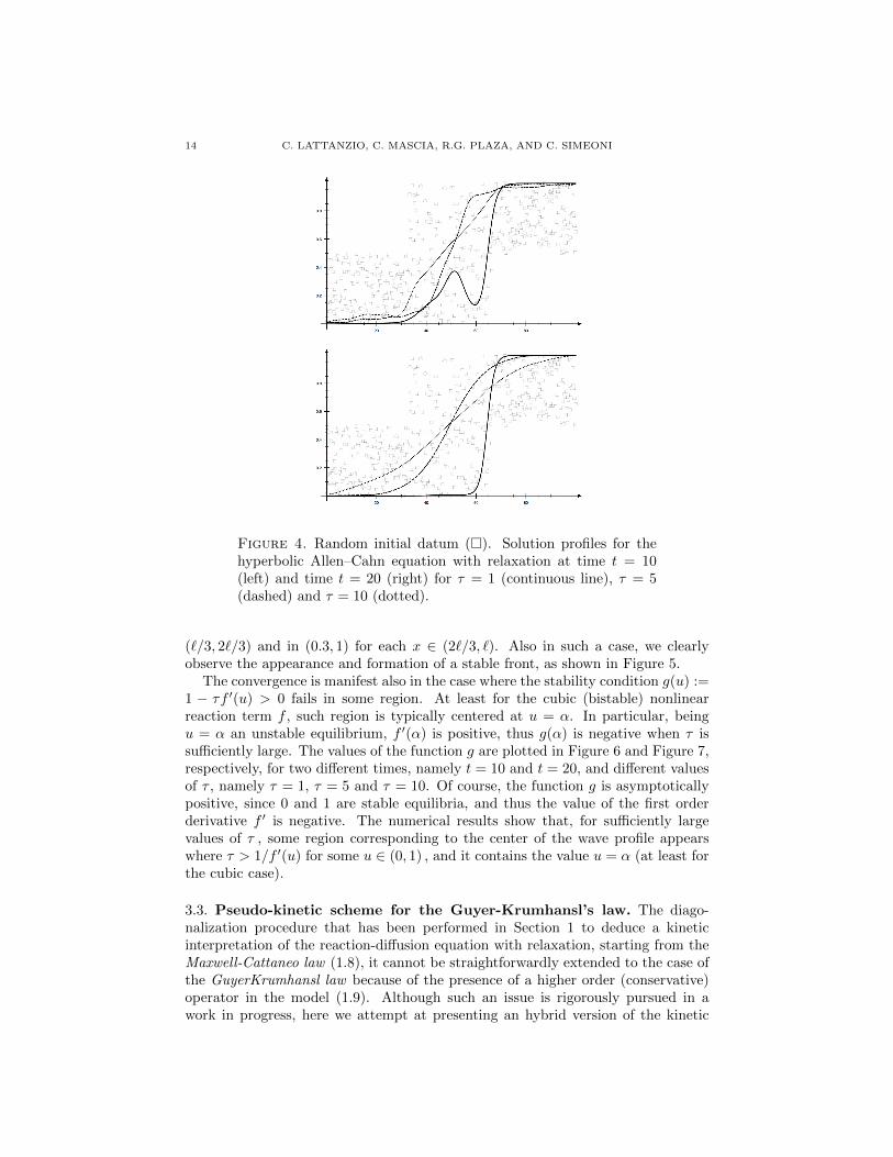
We consider initial data that resemble only very roughly the transition from 0 to1. More precisely, we divide the interval (0, `) into three parts of equal length andwe choose a random value in each of these sub-intervals coherently with the require-ment (3.2). We assign u0(x) to be any different random value in (0, 0.5) for eachx ∈ (0, `/3), in (0, 1) for each x ∈ (`/3, 2`/3) and in (0.5, 1) for each x ∈ (2`/3, `).Such choice can be considered as reasonable concerning the hypothesis (3.2), andthe results of the computation are shown in Figure 4.

The transition is even more robust than what the previous computation shows,since initial data that do not satisfy the requirement (3.2) still exhibits convergence.As an example, let us consider the case of a randomly chosen initial datum u0(x)given by any random value in (0, 0.7) for each x ∈ (0, `/3), in (0, 1) for each x ∈


Figure 4. Random initial datum (�). Solution profiles for thehyperbolic Allen–Cahn equation with relaxation at time t = 10(left) and time t = 20 (right) for τ = 1 (continuous line), τ = 5(dashed) and τ = 10 (dotted).

(`/3, 2`/3) and in (0.3, 1) for each x ∈ (2`/3, `). Also in such a case, we clearlyobserve the appearance and formation of a stable front, as shown in Figure 5.

The convergence is manifest also in the case where the stability condition g(u) :=1 − τf ′(u) > 0 fails in some region. At least for the cubic (bistable) nonlinearreaction term f , such region is typically centered at u = α. In particular, beingu = α an unstable equilibrium, f ′(α) is positive, thus g(α) is negative when τ issufficiently large. The values of the function g are plotted in Figure 6 and Figure 7,respectively, for two different times, namely t = 10 and t = 20, and different valuesof τ , namely τ = 1, τ = 5 and τ = 10. Of course, the function g is asymptoticallypositive, since 0 and 1 are stable equilibria, and thus the value of the first orderderivative f ′ is negative. The numerical results show that, for sufficiently largevalues of τ , some region corresponding to the center of the wave profile appearswhere τ > 1/f ′(u) for some u ∈ (0, 1) , and it contains the value u = α (at least forthe cubic case).

3.3. Pseudo-kinetic scheme for the Guyer-Krumhansl’s law. The diago-nalization procedure that has been performed in Section 1 to deduce a kineticinterpretation of the reaction-diffusion equation with relaxation, starting from theMaxwell-Cattaneo law (1.8), it cannot be straightforwardly extended to the case ofthe GuyerKrumhansl law because of the presence of a higher order (conservative)operator in the model (1.9). Although such an issue is rigorously pursued in awork in progress, here we attempt at presenting an hybrid version of the kinetic


Figure 5. Random initial datum (�) in (0, `). Solution profilesfor the hyperbolic Allen–Cahn equation with relaxation at timest = 10 (left) and t = 20 (right), for τ = 1 (continuous line), τ = 5(dashed) and τ = 10 (dotted).

scheme (2.6) to adapt to the present case, thus providing an easy-to-implementalgorithm for the pseudo-parabolic equation (1.13).

Starting from (2.6), we consider the following variation,

dvidt

= −%2 ui+1 − ui−12dxi

− 1

τvi +

(ν +

1

2%dxi

)vi+1 − 2vi + vi−1

dx2i

, (3.3)

that enjoys the same consistency properties as the original scheme, since the orderof magnitude of the physical parameter ν is clearly bigger than that of the correctionby the numerical viscosity 1

2%dx .Although it deserves to be rigorously justified and further confirmed by extensive

numerical simulations, this approach is clearly more convenient than the usual wayof putting higher order hyperbolic equations like (1.12) and (1.13) in form of lowerorder systems for numerical issues, namely

∂tu = w , τ∂tw +(1− τf ′(u)

)w − µ∂xxu+ ν ∂xxw = f(u) + ν ∂xxf(u) ,

for which a direct semi-discrete approximation provides duidt = wi , together with

τdwidt

= f(ui)−(1− τf ′(ui)

)wi + µ

ui+1 − 2 ui + ui−1

dx2 ,

− ν wi+1 − 2 wi + wi−1

dx2 + νf(u)i+1 − 2 f(u)i + f(u)i−1

dx2 .

(3.4)


Figure 6. Profile of the function g(u) := 1−τf ′(u) for time t = 10(left) and t = 20 (right) corresponding to the initial datum shownin Figure 4. The legend for the lines is the same as in the previousfigures.

Another way of dealing with higher order one-field equations can be the following:we rewrite (1.13) as

∂t(τ∂tu+ u− τf(u)− ν ∂xxu

)− µ∂xxu = f(u)− ν ∂xxf(u) ,

for which an alternative representation as second order system is given by

τ∂tu+ u− τf(u)− ν ∂xxu = w , ∂tw − µ∂xxu = f(u)− ν ∂xxf(u) ,

thus generalizing (1.5), with corresponding semi-discrete approximation

τduidt

= wi − ui + τf(ui) + νui+1 − 2 ui + ui−1

dx2 ,

dwidt

= f(ui) + µui+1 − 2 ui + ui−1

dx2 − νf(u)i+1 − 2 f(u)i + f(u)i−1

dx2 .

(3.5)

Both schemes (3.4) and (3.5) formally converge to the standard discretizationof (1.5) for τ → 0+ and ν → 0 , but they exhibit the well-known criticality of defin-ing the correct reconstruction of the external field f(u) on the (possibly nonuniform)spatial mesh. Therefore, the pseudo-kinetic scheme (3.3) maintains a wider interestin view of its underlying physical interpretation.

We conclude by remarking that such peculiar feature is not shared by other moregeneral forms of relaxation system, for instance

τ∂ttu+ g(t, x, u ; τ) ∂tu− µ∂xxu = f(u) , (3.6)


Figure 7. Profile of the function g(u) := 1−τf ′(u) for time t = 10(left) and t = 20 (right) corresponding to the initial datum shownin Figure 5. The legend for the lines is the same as in the previousfigures.

that is considered in [6], for example. Unless specific expression for the external fieldg are taken into account for physical reasons, the only approach to the numericalapproximation of (3.6) seems to be the transcription into a first order system byputting

∂tu = w , τ∂tw + g(t, x, u ; τ)w − µ∂xxu = f(u) .

On the other hand, under the hypothesis that g does not depend explicitly on theindependent variables, one can consider

g(u ; τ) ∂tu = ∂t(g(u ; τ)u

)− ∂ug(u ; τ)u ∂tu

and then equation (3.6) reads

∂t(τ ∂tu+ g(u ; τ)u

)− ∂ug(u ; τ)u ∂tu− µ∂xxu = f(u) ,

so that we can define

τ∂tu+ g(u ; τ)u = w , ∂tw − ∂ug(u ; τ)u ∂tu− µ∂xxu = f(u) ,

with the second equation rewritten like

∂tw −1

τ∂ug(u ; τ)u (w − g(u ; τ)u)− µ∂xxu = f(u)

that is even different from all the previous versions, thus revealing the great ad-vantage of a physical justification for the models at hands, as already suggested inSection 1.


Acknowledgements

This work has been partially supported by CONACyT (Mexico) and MIUR(Italy), through the MAE Program for Bilateral Research, grant no. 146529. Thework of RGP was partially supported by DGAPA-UNAM, grant IN100318.

References

[1] D. Bouche, J.-M. Ghidaglia, F. Pascal, Error estimate and the geometric corrector for theupwind finite volume method applied to the linear advection equation. SIAM J. Numer. Anal.

43 (2005), no.2, 578–603

[2] E. Bouin, V. Calvez, G. Nadin, Hyperbolic traveling waves driven by growth, Math. ModelsMethods Appl. Sci. 24 (2014), no. 6 (2014) 1165–1195

[3] V.A. Cimmelli, D. Jou, T. Ruggeri, P. Van, Entropy principle and recent results in non-equilibrium theories, Entropy 16 (2014) 1756–1807.

[4] F. Courchamp, L. Berec, J. Gascoigne, Allee effects in ecology and conservation, Oxford

University Press, Great Britain, 2008[5] P. C. Fife, J.B. McLeod, The approach of solutions of nonlinear diffusion equations to trav-

elling front solutions. Arch. Ration. Mech. Anal. 65 (1977) no. 4, 335–361

[6] R. Folino, C. Lattanzio, C. Mascia, Metastable dynamics for hyperbolic variations of Allen–Cahn equation, Commun. Math. Sci. 15 (2017), no.7, 2055–2085

[7] S. Gottlieb, C.W. Shu, Total variation diminishing Runge-Kutta schemes, Math. Comp. 67

(1998), no. 221, 73–85[8] B. Gustafsson, High order difference methods for time dependent PDEs, Springer Series in

Computational Mathematics 38, Springer-Verlag, Berlin, 2008

[9] K.P. Hadeler and J. Muller, Dynamical systems of population dynamics, in B. Fiedler (ed.),Ergodic theory, analysis, and efficient simulation of dynamical systems, Springer-Verlag,

Berlin, 2001[10] T.R. Hagen, M.O. Henriksen, J.M. Hjelmervik, K.-A. Lie, How to solve systems of conser-

vation laws numerically using the graphics processor as a high-performance computational

engine, in: G. Hasle, K.-A. Lie, E. Quak (Eds.), Geometric modelling, numerical simulation,and optimization: applied mathematics at SINTEF, Springer, Berlin, 2007, pp. 211–264

[11] A. Harten, S. Osher, Uniformly high-order accurate nonoscillatory schemes, SIAM J. Numer.

Anal. 24 (1987), no. 2, 279–309[12] T. Hillen, Invariance principles for hyperbolic random walk systems, J. Math. Anal. Appl.

210 (1997), no. 1, 360–374

[13] M.E. Hubbard, Multidimensional slope limiters for MUSCL-type finite volume schemes onunstructured grids, J. Comput. Phys. 155 (1999), no. 1, 54–74

[14] W.W. Hwu, GPU computing gems, Emerald & Jade Editions, Applications of GPU Com-

puting Series, Morgan Kaufmann Publishers, Elsevier, 2011[15] M. Kac, A stochastic model related to the telegrapher’s equation, Rocky Mountain J. Math.

4 (1974), 497–509

[16] Th. Katsaounis, C. Simeoni, Three-points interfacial quadrature for geometrical source termson nonuniform grids: application to finite volume schemes for parameter-dependent differen-

tial equations, Calcolo 49 (2012), no. 3, 149–176[17] D.B. Kirk, W.W. Hwu, Programming massively parallel processors: a hands-on approach,

Morgan Kaufmann Publishers, Elsevier, 2010[18] C. Lattanzio, C. Mascia, R.G. Plaza, C. Simeoni, Analytical and numerical investigation of

traveling waves for the Allen–Cahn model with relaxation, Math. Models Methods Appl. Sci.26 (2016), no.5, 931–985

[19] R.J. LeVeque, H.C. Yee, A study of numerical methods for hyperbolic conservation laws withstiff source terms. J. Comput. Phys. 86 (1990), no. 1, 187–210

[20] R.J. LeVeque, Finite volume methods for hyperbolic problems, Cambridge Texts in AppliedMathematics, Cambridge University Press, 2002

[21] F. Molna Jr., F. Izsak, R. Meszaros, I. Lagzi, Simulation of reaction-diffusion processes inthree dimensions using CUDA, Chemometrics and Intelligent Laboratory Systems 108 (2011)

76–85[22] L. Onsager, Reciprocal relations in irreversible processes I, Phys. Rev. 37 (1931), 405–426.


[23] A. Quarteroni, R. Sacco, F. Saleri, Numerical mathematics (second edition), Texts in Applied

Mathematics 37, Springer-Verlag, Berlin, 2007

[24] A.R. Sanderson, M.D. Meyer, R.M. Kirby, C.R. Johnson, A framework for exploring numeri-cal solutions of advection-reaction-diffusion equations using a GPU-based approach, Comput.

Vis. Sci. 12 (2009) 155–170

[25] C. Simeoni, Remarks on the consistency of upwind source at interface schemes on nonuniformgrids, J. Sci. Comput. 48 (2011), no.1-3, 333–338

[26] S. Tomov, R. Nath, H. Ltaief, J. Dongarra, Dense linear algebra solvers for multicore with

GPU accelerators, in: Proceedings of the 24th IEEE International Symposium on Parallel &Distributed Processing, IEEE Computer Society, Atlanta, 2010, 1–8.

(C. Lattanzio) Dipartimento di Ingegneria e Scienze dell’Informazione e Matematica,

Universita degli Studi dell’Aquila, via Vetoio (snc), Coppito I-67010, L’Aquila (Italy)E-mail address: [email protected]

(C. Mascia) Dipartimento di Matematica ‘G. Castelnuovo’, Universita di Roma ‘La

Sapienza’, Piazzale A. Moro 2, I-00185 Roma (Italy)E-mail address: [email protected]

(R. G. Plaza) Instituto de Investigaciones en Matematicas Aplicadas y en Sistemas,Universidad Nacional Autonoma de Mexico, Circuito Escolar s/n C.P. 04510 Cd. de

Mexico (Mexico)

E-mail address: [email protected]

(C. Simeoni) Laboratoire J.A. Dieudonne UMR CNRS 7351, Universite de Nice Sophia-

Antipolis, Parc Valrose 06108 Nice Cedex 02 (France)E-mail address: [email protected]

kinetic schemes for assessing stability of traveling

Documents