kinetic analysis of macromolecules: a practical approachgfit.sourceforge.net/refs/patel_transient...
TRANSCRIPT

Kinetic Analysis of Macromolecules: A Practical Approach
Editor: Kenneth A Johnson
Chapter Title
Transient-State Kinetics and Computational Analysis of
Transcription Initiation
Contributing Authors
Smita S. Patel1, Rajiv P. Bandwar, and Mikhail K. Levin
Robert Wood Johnson Medical School, Piscataway, New Jersey.
1Author for correspondence, Tel.: 732-235-3372; Fax: 732-235-4783; E-mail: [email protected].
Address: Department of Biochemistry, Robert Wood Johnson Medical School,
675 Hoes Lane, Piscataway, NJ 08854.
This research was supported by NIH grant GM51966 to SSP

1
1. Introduction
Transient-state kinetics is an important area of research to investigate the pathway of enzymatic
reactions (1-6). Specific experiments are designed to follow the formation and decay of reacting
species as a function of time. The concentrations are determined either directly by radiometric
methods or indirectly through optical changes associated with the formation of intermediates and
products. The kinetics is measured as a function of a second variable such as concentration of
enzyme or substrate, based on which a model or a kinetic pathway is constructed. The kinetic
data in most cases are too complex and hence best analyzed by computational methods that make
no assumptions in fitting the data, except for the model chosen by the investigator(7; 8). Several
types of experiments including kinetic and equilibrium types are globally fit using numerical and
least-squares fitting methods to derive a set of intrinsic rate constants that reveals the pathway of
the enzymatic reaction. The derived model is considered a working model that makes
predictions, based on which new experiments are designed. The results of these experiments are
used to refine the model.
In this chapter, we focus on how transient-state kinetic approaches can be used to elucidate the
dynamics of protein-DNA interactions and steps of promoter DNA melting, and RNA synthesis
catalyzed by a DNA-dependent RNA polymerase (RNAP1) during transcription initiation. In
addition we describe how MATLAB can be used to globally fit the kinetic data to obtain intrinsic
rate constants. The methods are described by focussing discussion on T7 RNAP, a single
subunit phage polymerase, that has been characterized extensively both structurally and
mechanistically (9-12). The bacteriophage RNAPs show similarity to mitochondrial and
chloroplast RNAPs(13), hence detailed studies of T7 RNAP can be valuable in understanding the
mechanism and regulation of transcription in higher organisms. The methods described here are
however general and applicable to studies of other enzymes and polymerases.
1Abbreviations: RNAP, RNA polymerase; 2-AP, 2-Aminopurine; nt, nucleotide; bp, base-pair; ss, single-stranded;ds, double-stranded; NT, non-template; T, template; PAGE, polyacrylamide gel electrophoresis; bis, N,N’-methylene-bis-acrylamide; BSA, bovine serum albumin; PMT, photomultiplier tube; NTP, nucleoside triphosphate; 3'-dGTP,3'-deoxyguanosine triphosphate; ODE, ordinary differential equation; JSP, Jacobian sparcity pattern.

2
1.1 RNA polymerase
DNA-dependent RNAPs are key enzymes engaged in transcription during which RNA is made
by condensing individual rNTPs as directed by the sequence of the genomic DNA. Transcription
is a complex process that can be divided into several stages: a) initiation, b) abortive RNA
synthesis, c) promoter clearance, d) elongation, and e) termination (14; 15). During transcription
initiation, the RNAP recognizes and binds to a specific dsDNA promoter sequence, a short
stretch of which is unwound in the vicinity and including the RNA synthesis start site. The
exposed bases of the template strand direct binding of two initiating rNTPs at the polymerase
active site. RNA synthesis begins by the formation of a phosphodiester bond between the
initiating rNTPs resulting in the shortest RNA, pppNpN. RNA synthesis continues with
sequential addition of rNMPs to the 3'-OH of the terminal nucleotide of the RNA. In the early
stages of transcription, when the RNAP is still bound to the promoter, short RNAs (up to 12-
mer) tend to dissociate as abortive products. When the RNAP clears the promoter, transcription
goes into the elongation phase during which RNA synthesis occurs in an efficient and processive
manner.
Transcription is a key process by which RNAs that code for proteins, structural RNAs such as
ribosomal RNA, and tRNAs are synthesized. Regulation of transcription is therefore critical for
controlled cell growth and development. Each stage of transcription is regulated by interactions
of the RNAP with the DNA, by accessory proteins such as transcription factors, and by ligands.
The promoter sequence plays a critical role in regulating the steps of transcription initiation.
Any of the multiple steps of initiation can be modulated to control the efficiency of RNA
synthesis. However, the rate limiting steps and steps with unfavorable equilibrium constants
when regulated are expected to have the greatest effect. To understand transcription regulation,
it is important to first elucidate the kinetic pathway of the process and this can be done by
dissecting the elementary steps, determining their intrinsic rate constants, and then determining
which steps are affected by promoter sequence variation or by accessory factors.

3
1.2. Minimal Pathway
With existing knowledge the investigator can write a minimal pathway of the reaction. For
instance, the minimal pathway of transcription initiation up to the step of first phosphodiester
bond formation reaction is written below:
Reaction 1:
Where E is T7 RNAP, and D is a dsDNA promoter that forms a closed complex, ED, upon
binding to T7 RNAP. The closed complex then isomerizes to an open complex, EDo, in which
–4 to +2 region of the dsDNA is unwound, and one of the strands of the melted DNA serves as a
template for RNA synthesis. Two initiating GTPs bind at the active site of the EDo complex
directed by the sequence of the start site (+1GGG). The phosphodiester bond formation reaction
follows resulting in the synthesis of the first RNA product pppGpG.
2. Experimental Approach
The challenge lies in designing experiments to measure each step in the enzymatic pathway in
order to dissect the intrinsic rate constants (k1 through k6). We describe two types of methods
that were used to obtain the intrinsic rate constants of the transcription initiation pathway. The
initial steps of RNAP binding to the promoter DNA that result in a preinitiation open complex
were measured by stopped-flow fluorescence method. The steps of initiating nucleotide binding
and RNA synthesis were measured by both stopped-flow fluorescence and radiometric rapid
chemical-quench-flow methods. We emphasize that two or more types of kinetic experiments
should be used in conjunction to derive the rate constants and the data should be globally fit to
dissect the complete pathway.
E + D ED EDo EDoG EDoGG EDopppGpGGTP GTPk1
k2
k3
k4 Kd1,GTP Kd2,GTP
k5
k6

4
Both RNAP and the promoter dsDNA undergo conformational changes upon forming a binary
complex and during subsequent steps of transcription. To follow the steps of DNA binding and
conformational changes, one can monitor either the change in the intrinsic fluorescence of
protein residues (tryptophan and tyrosine) upon DNA binding or label the protein or the
promoter DNA with a probe whose fluorescence is sensitive to structural or environmental
changes. The transient fluorescent changes can be measured in real-time starting from msec to
sec after rapidly mixing RNAP with the DNA in a stopped-flow instrument. The observed
kinetics is then analyzed to obtain information about the number of steps in the pathway and
their intrinsic rate constants. To monitor the steps of rNTP binding and RNA synthesis,
experiments can be designed in which the RNAP and DNA are incubated to pre-form the open
complex prior to mixing with rNTPs. By following the synthesis of RNA under presteady-state
conditions, one can measure both the Kd values of rNTPs and the intrinsic rates of RNA
synthesis. Typically this reaction is carried out in a rapid chemical-quench-flow apparatus that
allows rapid mixing of the reacting species and quenching the reaction in as short as 2 msec after
mixing. This is a discontinuous assay and when radiolabeled rNTPs are used, RNA synthesis is
quantified after the products are resolved by sequencing PAGE.
2.1 Fluorimetric methods
T7 RNAP has 19 tryptophans and 24 tyrosines and when it binds the promoter DNA there is a
net decrease in the intrinsic fluorescence of these residues, although the decrease is very
small(16). Sensitive instrumentation and data averaging can be used to follow even small
changes in fluorescence over time to measure the kinetics of DNA binding. The origin of protein
fluorescence change is complex; hence, the fluorescence changes cannot be interpreted in terms
of the structure of the intermediates.
The normal bases in the DNA have very short decay times, typically few picoseconds, which
results in a very weak intrinsic fluorescence of DNA. This hampers the use of normal DNA for
studying DNA-protein interactions by fluorimetric methods and to monitor structural changes in
the DNA within the confines of the protein-DNA complex. Therefore much useful kinetic and

5
Figure 1: (A) Synthetic oligodeoxy-nucleotidescontaining the consensus T7 promoter sequence.The 40-bp dsDNA sequence is the φ10 promotersequence from –21 to +19 relative totranscription start site at +1. The 17/40 p-dsDNA is single stranded in the initiation andcoding regions from –4 to +19. (B) Fluorescentbase analogs 2-AP and pyrrolo-dC. 2-AP formsWatson-Crick base pair with T and has anexcitation and emission maxima of 305 nm and370 nm respectively. Pyrrolo-dC base pairs withG and has an excitation and emission maxima of350 nm and 460 nm, respectively.
structural information pertaining to DNA, viz. melting, twisting, etc., can not be obtained.
Substitution of a normal base by a modified structural analog possessing fluorescent properties
can provide an important handle to study protein-DNA interactions by fluorimetric methods. 2-
Aminopurine and pyrrolo-dC are fluorescent analogs of adenine and cytosine, respectively (17-
20) that can be selectively excited in the presence of tryptophan and tyrosine protein residues.
Both probes form stable Watson-Crick type base pair (Figure 1), and 2-AP:dT bp does not
perturb the B-helical structure of the duplex DNA. Their fluorescence is highly sensitive to
base-stacking interactions and placement of these analogs at chosen positions in the DNA helix
allow measurement of local events such as binding of DNA to proteins, conformational changes
in DNA, melting transitions, etc (21-29). These fluorescent changes have been measured both in
real-time and at steady-state to determine the kinetics and thermodynamics of promoter DNA
binding and promoter strand separation processes of transcription initiation(16; 22; 23; 28; 29).
2.2 DNA
2.2.1 Purification and concentration determination. The oligodeoxynucleotides of predefined
sequences either unmodified or modified with 2-AP are chemically synthesized. The ssDNAs
are purified by PAGE using Protocol 1. The concentration of ssDNA is determined by
absorbance measurement (Protocol 1), and the dsDNA is prepared by annealing complementary
ssDNA strands. Studies with two types of promoter DNAs are described (Figure 1). The p-
dsDNA has a duplex promoter binding region and single stranded melting and coding regions.
+1
N
N
N
N
N
dR H
H
NN
O
O
CH3
H dR
2-AP:T
N
N
N
N
N
O
dR
H
H
H
N N
N
O
dR
H
H3C
G:pyrrolo-dC
A
B
40-bp dsDNA
17/40 p-dsDNA
5'-AAATTAATACGACTCACTATAGGGAGACCACAACGGTTTC-3'3'-TTTAATTATGCTGAGTGATATCCCTCTGGTGTTGCCAAAG-5'
5'-AAATTAATACGACTCAC-3'3'-TTTAATTATGCTGAGTGATATCCCTCTGGTGTTGCCAAAG-5'

6
This DNA is used as a mimic of the open DNA that is generated during open complex formation.
The 40-bp dsDNA is a fully duplex promoter with T7 promoter consensus sequence (30).
Protocol 1. Purification of synthetic oligodeoxynucleotides
Equipment and reagents
• 180 mm x 320 mm glass plates, 3 mm thick spacers and single well combs, and electrophoresisapparatus
• UV lamp (MINERALIGHT lamp, Model UVGL-25, Multiband UV-254/366 nm)
• Kodak Biomax MS screen for gel viewing under UV light
• S&S ELUTRAP Electro-separation system and accessories.
• 16 % (w/v) acrylamide solution (150 ml for each gel) in 1x TBE containing 4M Ureaa
• One µmole desalted single stranded oligodeoxynucleotides modified with single internal 2-AP (thiscan be commercially obtained by custom synthesis from various companies or DNA synthesis labs)
• Sequencing gel loading buffer, and 1x TBE
Method
1. Prepare 16% acrylamide denaturing gelsb using 180 mm x 320 mm plates and 3mm spacers andcombs.
2. Set the temperature of the electrophoresis chamber (filled with 1x TBE) to ~ 60 °C (optional).
3. Load the DNA dissolved in 100 µl de-ionized water and an equal volume of sequencing gel loadingbuffer on the gel.
4. Run the gel at 350-400 V until the dye front reaches the bottom of the gel (this may take 6-7 hdepending on the applied voltage).
5. Visualize the DNA under short UV light using Kodak screen as background, and cut out the mostintense band from the gel.
6. Electroelute the ssDNA from the gel using ELUTRAP Electro-separation system.
7. Ethanol precipitate the electroeluted DNA (Note: we omit the 70 % EtOH treatment for smallerssDNAs (< 40 nt) to avoid loss of DNA).
8. Resuspend the dried DNA pellet in 100-150 µl de-ionized water and measure the concentration usingabsorbance at 260 nm (A260) and calculated extinction coefficient (dA = 15,200, dT = 8,400, dG =12,010, dC = 7,050 and 2-AP = 1,000 M-1cm-1).
a Acrylamide is potentially neurotoxic, see ref. (31) for handling instructions.b For preparation of denaturing PAGE, see ref. (31)
____________________________________________________________________________________

7
C
0
25
50
75
100
-4T -3NT -2T -1NT +4NT
2-AP position
-1-3
-4 -2
+4-21 +19A
B
Wavelength (nm)360340 400380 420
dsDNA
2-AP DNA
ssDNA
ssDNAdsDNA
Fluo
resc
ence
(x 1
0) c
ps5
Fluo
resc
ence
(x 1
0) c
ps4
5’-AAATTAATACGACTCACT T GGG GACCACAACGGTTTC-3’(NT)3'-TTTAATTATGCTGAGTG T TCCCTCTGGTGTTGCCAAAG-5’(T)
A A AA A
2.2.2 Incorporation of 2-AP in the DNA and its fluorescent properties. The preferred position to
incorporate 2-AP in the DNA in order to monitor the events of promoter strand separation is in
the region that gets unwound during initiation. This region in most promoters is A/T rich and
hence individual adenines in this region can be substituted with 2-AP. In T7 promoter, the –4 to
+2 region of the promoter (numbering relative to transcription start site at +1) is unwound during
preinitiation open complex formation (32). Hence, 2-AP was singly incorporated in place of
adenines at positions –1NT, -3 NT, +4 NT, -2 T or -4 T (Figure 2A). The absorption and emission
spectra of these DNAs are measured both in ssDNA and dsDNA forms, and compared to one
another (22). The position of probe in the DNA does not affect the absorption spectra of the 2-
AP modified DNAs that exhibit a strong peak at 260 nm, corresponding to the absorption of
normal bases, and a shoulder in the region 305-315 nm, corresponding to 2-AP absorption.
Upon excitation at 315 nm, the 2-AP modified ssDNA show a broad fluorescence spectrum, with
a peak at 370±1 nm (Figure 2B). The fluorescence of 2-AP in ssDNA is quenched when the
ssDNAs are annealed with their complementary strands. On an average, the fluorescence of free
2-AP base is quenched ~95 % upon incorporation into ssDNA and a further 30-90 % quenching
Figure 2: (A) The 40-bp dsDNA promoter showing the positions of single 2-AP substitutions either in thenon-template (NT) or the template (T) strand. (B) Typical fluorescence emission spectra of singly 2-APsubstituted ssDNA and dsDNA upon excitation at 315 nm. (C) Fluorescence intensities of the five singly2-AP substituted promoter strands both in the ssDNA and dsDNA form (1 µM each) measured at 370 nmafter excitation at 315 nm at 25 °C.
8
Time (min)0 5 10 15 20 25 30
0
1
2
3
4
5 Exonuclease contaminated T7 RNAPPure T7 RNAP
Fluo
resc
ence
(x 1
0) c
ps6
is observed when the ssDNA is converted to dsDNA. Therefore, the 2-AP fluorescence is
sensitive to the structure of the DNA, with the fluorescence of 2-AP being higher in the ssDNA
versus the dsDNA. The 2-AP fluorescence in ssDNA is influenced by the neighboring bases as
shown in Figure 2C (22). When the 2-AP base is flanked by two guanines, the fluorescence of
ssDNA or dsDNA is the least (at position +4 NT). When 2-AP is adjacent to a single guanine, the
fluorescence is intermediate (at -1 NT and -4 T), and when the flanking bases are not guanine, then
the fluorescence is the highest (at -2 T and -3 NT). Thus, guanine residues quench the
fluorescence of 2-AP, especially when the 2-AP is stacked next to the guanine.
2.3. Protein
2.3.1 Concentration determination and purity. T7 RNAP is purified to homogeneity (33) and
protein concentration is determined both by Bradford assay (34) and by light absorbance at 280
nm (35) (extinction coefficient of T7 RNAP, 1.4 x 10⁵ M-1cm-1). The extinction coefficient of
the protein can be calculated from the protein sequence using the ProtParamtool
(http://www.expasy.ch/tools/protparam.html). The choice of protein standard in the Bradford
assay is important and most investigators use BSA as a standard. It is important to verify that
both methods of protein concentration determination (Bradford and light absorption) provide
consistent results.
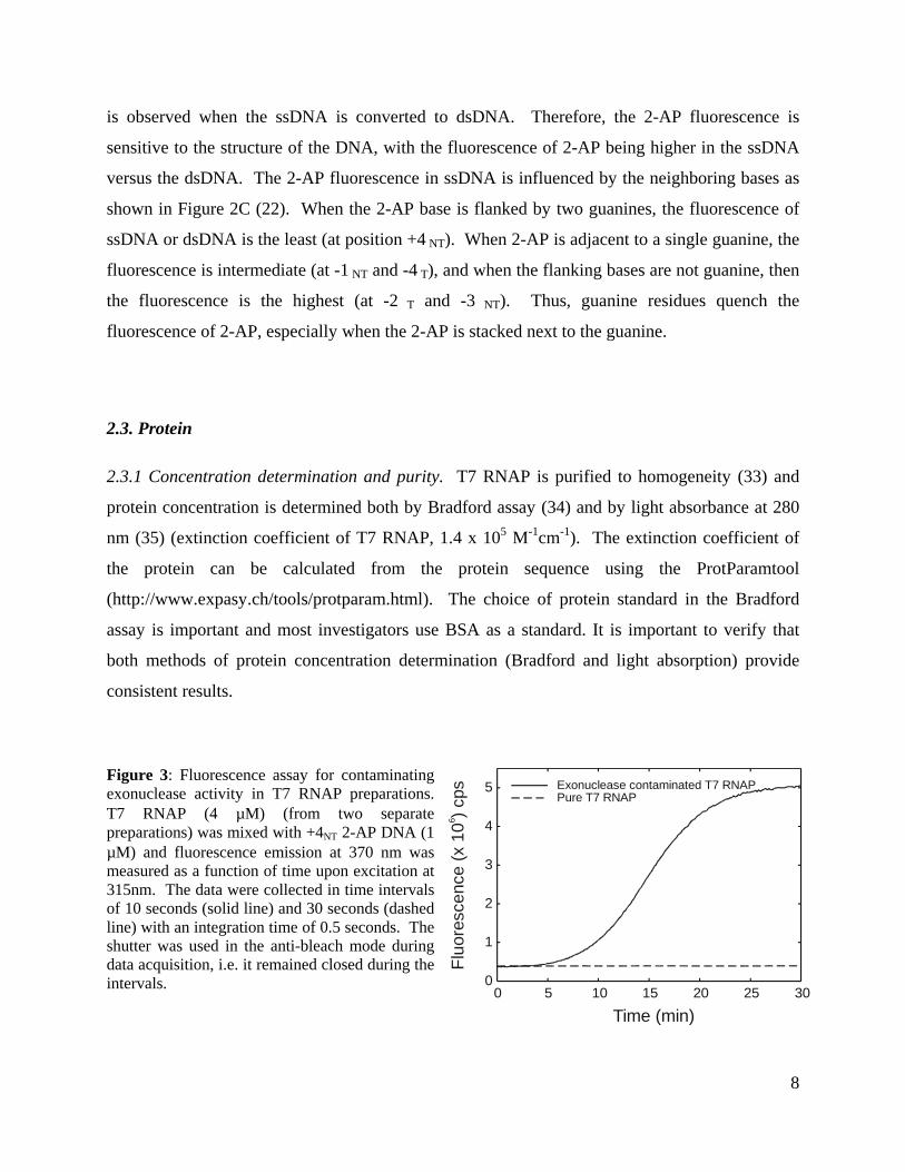
Figure 3: Fluorescence assay for contaminatingexonuclease activity in T7 RNAP preparations.T7 RNAP (4 µM) (from two separatepreparations) was mixed with +4NT 2-AP DNA (1µM) and fluorescence emission at 370 nm wasmeasured as a function of time upon excitation at315nm. The data were collected in time intervalsof 10 seconds (solid line) and 30 seconds (dashedline) with an integration time of 0.5 seconds. Theshutter was used in the anti-bleach mode duringdata acquisition, i.e. it remained closed during theintervals.

9
The protein preparation is checked for purity by SDS PAGE. Even though the protein may
appear pure, there may be contaminating DNA exonuclease amounts undetectable by PAGE.
Contaminating exonuclease presence produce artifacts in the fluorescence measurements because
the fluorescence of 2-AP increases greatly when the base is excised from the DNA. The 2-AP
fluorescence increase due to contaminating exonuclease activity can be mistaken as a
fluorescence change arising from promoter opening or protein-DNA binding. The fluorescence
assay described in Protocol 2 provides a convenient method for checking the presence of any
contaminating exonuclease activity. A time course of fluorescence increase is shown in Figure 3
for preparations of T7 RNAP with and without contaminating exonuclease. If protein
preparations are found to contain exonuclease, they are further purified before use.
Protocol 2. Fluorescence assay for exonuclease activity.
Equipment and reagents
• Fluorescence spectrophotometer (preferably equipped with a stirrer and programmable to measure
fluorescence as a function of time).
• 2-AP containing DNA, and protein sample.
• 5x Reaction buffer (1x concentrations = 50 mM Tris-acetate, pH 7.5, 50 mM Na-acetate, 10 mM Mg-
acetate, 5 mM DTT).
Method
1. Prepare 0.1 to 1 µM 2-AP DNA solution in 1x reaction buffer and measure fluorescence at 370 nm
after exciting at 315 nm.
2. Add an aliquot of the protein solution and measure the fluorescence as a function of time, from min to
few hours. Keep the shutter closed between measurements to minimize photo-bleaching.
3. Plot observed fluorescence as a function of time (see Figure 3).
______________________________________________________________________________

10
3. Equilibrium Fluorescence Measurement
3.1 Fluorescence of T7 RNAP-DNA complex
The fluorescence changes in each of the five dsDNA promoters containing 2-AP at various
positions was measured in the presence of T7 RNAP and corrected as described in Protocol 3B.
Upon complex formation, the fluorescence intensity of 2-AP DNA increases (Figure 4A) (22;
28). The fluorescence change in DNA containing 2-AP at positions –4 to –1 is significantly
higher than the fluorescence change at +4 NT (Figure 4B). The fluorescence of 2-AP incorporated
in the DNA increases when the 2-AP base unstacks from the helix (19). The results indicate that
the +4 bp is not significantly perturbed (unpaired or unstacked) in the preinitiation open complex.
The 2-AP fluorescence at -1 NT, -3 NT, -4 T, and -2 T positions increase to different extents in the
binary complex (Figure 4B). A peculiarly large increase in the fluorescence of 2-AP at -4 T was
observed in the binary complex (about 20-fold from free dsDNA fluorescence compared to 3 to 4
fold increase at the other three positions) (22).
Figure 4: (A) Typical fluorescence emission spectra of the 40-bp dsDNA upon addition of T7 RNAPupon excitation at 315 nm. (B) Fluorescence (excitation, 315 nm and emission, 370 nm) intensity of the40-bp dsDNA promoter (five singly 2-AP substituted dsDNAs at 0.5 µM) upon addition of T7 RNAP (4.0µM). The five 2-AP positions are indicated in Figure 2A. The observed fluorescence intensities werecorrected for inner-filter effect and subtracted from the fluorescence of T7 RNAP-DNA complex formedusing normal dsDNA (non 2-AP DNA) to correct for fluorescence contribution from excess T7 RNAP.
2-AP position
0
5
10
15
20
dsDNA dsDNA + RNAP
-4T -3NT -2T -1NT +4NT
B
Wavelength (nm)340 360 380 400 420
0
5
10
15
20
25
30 dsDNA+ RNAP
dsDNA
A
Fluo
resc
ence
(x 1
0) c
ps4
Fluo
resc
ence
(x 1
0) c
ps4

11
The increase in fluorescence of 2-AP at -4T was observed also in the p-dsDNA (22). Although
the 2-AP at -4T is already unpaired in the p-dsDNA, the base unstacks during open complex
formation (32). The unstacking of –4T 2-AP base from the adjacent guanine at -5T, which
quenches the fluorescence of the stacked 2-AP base, results in fluorescence increase observed in
the p-dsDNA upon binding to T7 RNAP.
3.2 Equilibrium dissociation constant
The fluorescence changes in 2-AP containing dsDNA promoters upon forming a complex with
T7 RNAP can be used to measure the equilibrium dissociation constant or Kd of promoter DNA
(Protocol 3C). In the fluorimetric titration, a constant amount of T7 RNAP is titrated with
increasing concentration of 2-AP modified DNA, and the fluorescence of 2-AP DNA is
measured at equilibrium. The fluorescence is corrected for volume changes and inner filter
effect using Eqn 1.
+
×
×= emAbsexAbs.
ovfv
obsFcF50
10 (Eqn. 1)
Where, Fc is corrected fluorescence, Fobs is the observed fluorescence intensity, vf is the final
volume of the solution, vo is the initial volume, Absex the absorbance of the T7 RNAP-DNA
solution at the 2-AP excitation wavelength of 315 nm, and Absem the absorbance of the same
solution at the 2-AP emission wavelength of 370 nm. The corrected fluorescence is plotted as a
function of total [DNA] and fit to Eqn. 2-3 to obtain the DNA Kd value (Figure 5).
( )DDbDc ffEbDfCF −×+×+= (Eqn. 2)
Where C is a constant, fD is a fluorescence coefficient for free 2-AP DNA, D is total [DNA], fDb
is a fluorescence coefficient for T7 RNAP-DNA complex, and Eb is the concentration of protein-
DNA complex defined by Eqn. 3.
( )2
42 DEtDEtKDEtKEb dd ××−++−++
= (Eqn. 3)
Where D is total [DNA], Et is total [T7 RNAP], and Kd is dissociation constant.
12
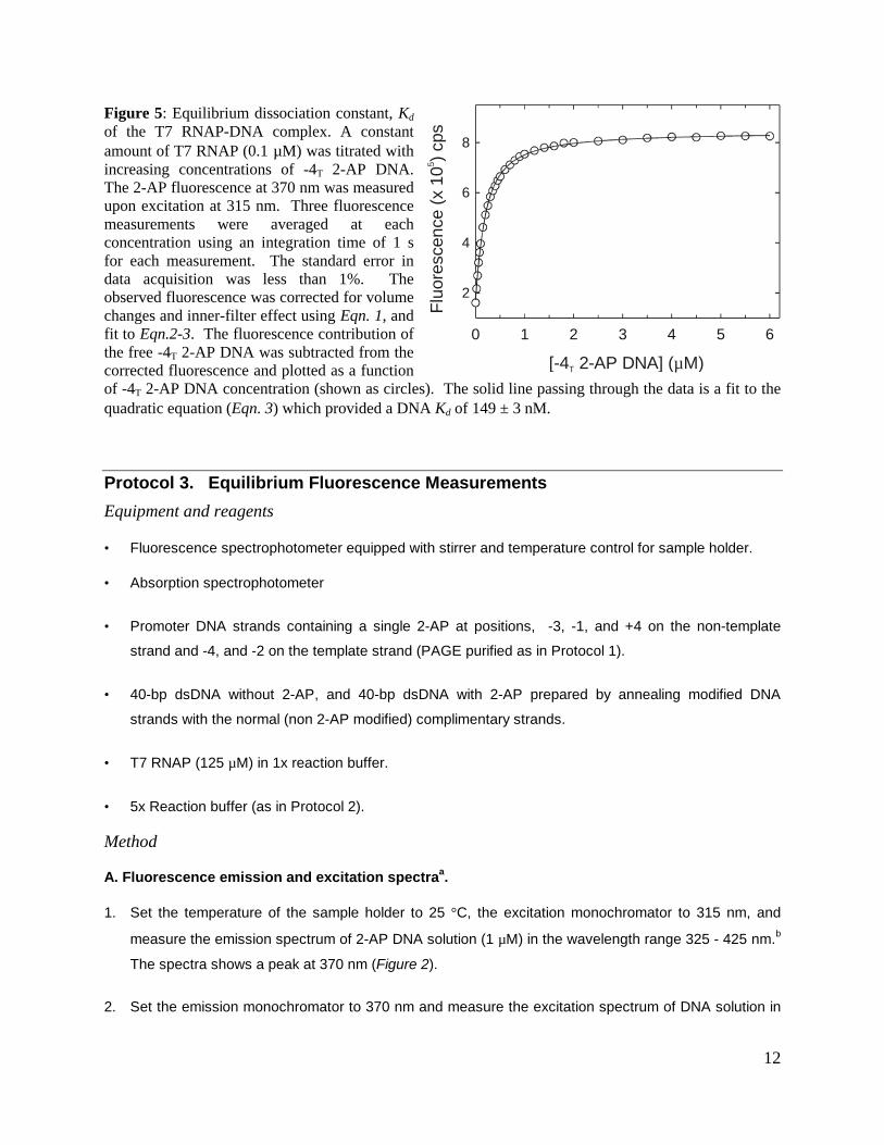
Figure 5: Equilibrium dissociation constant, Kd
of the T7 RNAP-DNA complex. A constantamount of T7 RNAP (0.1 µM) was titrated withincreasing concentrations of -4T 2-AP DNA.The 2-AP fluorescence at 370 nm was measuredupon excitation at 315 nm. Three fluorescencemeasurements were averaged at eachconcentration using an integration time of 1 sfor each measurement. The standard error indata acquisition was less than 1%. Theobserved fluorescence was corrected for volumechanges and inner-filter effect using Eqn. 1, andfit to Eqn.2-3. The fluorescence contribution ofthe free -4T 2-AP DNA was subtracted from thecorrected fluorescence and plotted as a functionof -4T 2-AP DNA concentration (shown as circles). The solid line passing through the data is a fit to thequadratic equation (Eqn. 3) which provided a DNA Kd of 149 ± 3 nM.
Protocol 3. Equilibrium Fluorescence Measurements
Equipment and reagents
• Fluorescence spectrophotometer equipped with stirrer and temperature control for sample holder.
• Absorption spectrophotometer
• Promoter DNA strands containing a single 2-AP at positions, -3, -1, and +4 on the non-template
strand and -4, and -2 on the template strand (PAGE purified as in Protocol 1).
• 40-bp dsDNA without 2-AP, and 40-bp dsDNA with 2-AP prepared by annealing modified DNA
strands with the normal (non 2-AP modified) complimentary strands.
• T7 RNAP (125 µM) in 1x reaction buffer.
• 5x Reaction buffer (as in Protocol 2).
Method
A. Fluorescence emission and excitation spectraa.
1. Set the temperature of the sample holder to 25 °C, the excitation monochromator to 315 nm, and
measure the emission spectrum of 2-AP DNA solution (1 µM) in the wavelength range 325 - 425 nm.b
The spectra shows a peak at 370 nm (Figure 2).
2. Set the emission monochromator to 370 nm and measure the excitation spectrum of DNA solution in
0 1 2 3 4 5 6
2
4
6
8
Fluo
resc
ence
(x 1
0) c
ps5
[-4 2-AP DNA] ( M)T µ

13
the wavelength range 250 - 350 nm. A peak at 305 nm is observed.
3. Measure the fluorescence of T7 RNAP alone, and then the fluorescence of T7 RNAP (1 to 4 µM)
added to the solution of 2-AP dsDNA. (It is advisable to add a sufficiently concentrated solution of T7
RNAP so that the volume change is relatively small, < 5 % of the initial volume).
B. Fluorescence of T7 RNAP- 2-AP DNA complex
1. Use the constant wavelength analysis mode for data acquisition and set excitation and emission
wavelengths of 315 nm and 370 nm, respectively.
2. Measure the fluorescence of 2-AP DNA (1 µM). Add T7 RNAP (4 µM) in a small volume and
measure the fluorescence. Correct for volume and inner filter using Eqn. 1 (Fc(f))
3. Repeat step (2) with the non 2-AP DNA (Fc(nf)).
4. The fluorescence intensity of T7 RNAP-2-AP DNA complex is determined as shown in Figure 4 usingthe following equation: Fluorescence = Fc(f) – Fc(nf).
C. Fluorimetric titration
1. Set up the fluorimeter as in Protocol 3B, step 1.
2. Prepare 2500 µl 1x reaction buffer, transfer to cuvette with a small stir bar, and measure the
fluorescence at 370 nm.
3. Measure the absorbance of buffer as a reference (baseline) at wavelengths 315 and 370 nm in the
same cuvette.
4. Add 2.0 µl of T7 RNAP solution (125 µM) (final T7 RNAP concentration is 0.1 µM) and note the final
volume (i.e. 2502 µl). Stir and after 2 min measure both fluorescence and absorbance values.
5. Add 2 µl increments of 2-AP DNA (from a stock 25 µM) until the final concentration DNA is 0.1 µM.
Continue adding 5 µl increments, up to 0.5 µM, 10 µl increments up to 1.0 µM. Stir for 2 min (or
longer to reach equilibrium) and measure the fluorescence and absorbance after each addition of
DNA.
6. Add 4 µl increments of 2-AP DNA (from a stock 125 µM) until the final concentration of DNA is 1 µM.
Continue adding 10 µl increments, up to 6 µM.
7. Use Eqn. 1 to correct the observed fluorescence values for volume changes and inner filter effect.

14
CkteAy +
−−×= 1
8. Plot the corrected fluorescence (Fc) as a function of [DNA]. The Fc at high concentration of DNA is
linear and corresponds to free 2-AP DNA.
9. Using Eqn. 2 and 3 fit the Fc vs. [DNA] plot to obtain the Kd of the T7 RNAP-DNA complex.
10. Subtract the fluorescence contribution of the free 2-AP DNA from the Fc using the equation, Fc - fD ×[DNA] and re-plot slope corrected Fc vs. [DNA] (as shown in Figure 5).
a It is assumed that the researcher is familiar with the normal operation of the fluorescence instrument so
only required settings are provided, otherwise follow instrument instruction guidelines for standard
operational procedures.
b Place the cuvette in the same orientation throughout the experiment to maintain consistency during data
acquisition.
_____________________________________________________________________________
4. Kinetics of RNAP and promoter DNA binding
4.1 Stopped-flow kinetics of p-dsDNA binding
To measure the kinetics of p-dsDNA interaction with T7 RNAP, a known concentration of the p-
dsDNA is mixed with excess T7 RNAP in a stopped-flow instrument (Protocol 4) and the time-
dependent increase in fluorescence is measured (Figure 6). The kinetics measured under pseudo
first-order conditions (one reacting species in excess of the other) fit well to a single exponential
(Eqn. 4). The time courses are measured at various concentrations of T7 RNAP and each time
course is fit to Eqn. 4.
(Eqn. 4)
Where y is observed fluorescence, A is fluorescence change, t is time, k is rate constant, and C is
y-intercept.

15
Figure 6: (A) Stopped-flow setup. (B) Stopped-flow kinetics of 17/40 2-AP p-dsDNA binding to T7RNAP measured at 25 °C. The sequence of 17/40 p-dsDNA is shown in Figure 1A. A constant amount(0.05 µM final) of -4T 2-AP p-dsDNA was mixed with varying concentrations (0.2 - 0.5 µM final) of T7RNAP, and the time-dependent fluorescence change (λ > 360 nm) was monitored after excitation at 315nm. Kinetic traces (5-7) were averaged at each concentration.
The observed rates are plotted versus [T7 RNAP] (Figure 7A), which show a linear dependency.
The interpretation of this result is straightforward and consistent with a one-step model (Reaction
2):
Reaction 2:
If the experiments are carried out under pseudo first-order conditions the linear dependency can
be fit to Eqn 5 to obtain k1 (2.6 x 10 8 M-1s-1) and k2 (close to zero).
kobs = k1[E] + k2 (Eqn. 5)
The dependency shows that the value of k1 is determined with greater accuracy than k2, because,
for practical reasons, data cannot be collected for concentrations where the observed rates would
be close to k2. The value of k2 or the dissociation rate constant of p-dsDNA from T7 RNAP in
such a case is measured directly.
E + D EDk1
k2
PMT
315 nm
> 360 nm
2-APDNARNAP
A
0.1 1 10 100
4.6
4.8
5.0
5.2
5.4
5.6
Time (ms)
B
0.5 µM0.4 µM0.4 µM0.3 µM0.2 µMFl
uore
scen
ce (>
360
nm
)
[T7
RN
AP
]

16
Time (min)0 30 60 90 120 150 180
Fluo
resc
ence
(x 1
05 ) cps
2.40
2.45
2.50
2.55
2.60
[T7 RNAP] (µM)
0.0 0.1 0.2 0.3 0.4 0.5 0.6
Obs
erve
d ra
te (s
-1)
0
25
50
75
100
125
150
A B
Figure 7: (A) The on-rate of 17/40 p-dsDNA binding to T7 RNAP. The kinetic traces (Figure 6B) werefit to Eqn. 4 and the observed rates are plotted as a function of [T7 RNAP] (circles). The observed rate vs[T7 RNAP] plot was fit to Eqn. 5 with k1 (= kon) of 260 ± 3 µM-1s-1 and k2 (=koff) close to zero. (B) Theoff-rate of 17/40 p-dsDNA-RNAP complex was measured by mixing at time zero 0.05 µM RNAP-pDNAcomplex (0.05 µM T7 RNAP + 0.1 µM -4T 2-AP p-dsDNA) with 2 µM non-fluorescent p-dsDNA in astandard fluorescence cuvette. Time-dependent fluorescence decrease at 370 nm (upon excitation at 315nm) was monitored (circles). Three measurements were averaged at each time with an integration time of0.5 s for each measurement. The shutter was used in the anti-bleach mode during data acquisition. Thefluorescence decrease was fit Eqn. 6 that provided koff of 0.00034 s-1 (solid line). Thus the overall Kd (=koff/kon) of T7 RNAP-p-dsDNA complex is 1.3 pM.
4.2 Dissociation rate constant
T7 RNAP and p-dsDNA (2-AP modified) is mixed with excess of unmodified p-dsDNA and the
decrease in fluorescence with time is measured. The rationale behind this experiment is that
when the fluorescent p-dsDNA dissociates from T7 RNAP, it gets diluted in a pool of excess
nonfluorescent p-dsDNA. The chances of a fluorescent DNA rebinding the enzyme are very
small; hence, the decrease in fluorescence with time is fit to an exponential Eqn. 6 to estimate the
value of k2.
(Eqn. 6)
This experiment can be carried out in a stopped-flow instrument (if the
dissociation rates are >0.01 s-1, half-life <60 s) or in fluorimeter (if the dissociation rates are
<0.01 s-1). The dissociation rate of p-dsDNA was measured to be 3.4 x 10⁻⁴ s-1 and measured in a
fluorimeter (Figure 7B). With slow dissociation rates, it is important that sample is exposed to
light intermittently to minimize photobleaching.
CkteAy +
−×=
17
Protocol 4. Measurement of fast kinetics by the stopped-flow method.
Equipment and reagents
• Stopped-flow instrument equipped with a 75W Xenon lamp and excitation monochromator (Model:
SF-2001 from KinTek Corporation, Austin, TX), 360 nm cut-off filter
• 5x reaction buffer (as in Protocol 2). All dilutions are made in 1x reaction buffer.
• 2-AP DNA modified at –4T (0.1 µM)
• 2-AP DNA modified at +4NT (0.6 µM)
• T7 RNAP (25 µM and 1.8 µM)
• GTP (12.5 mM)
Methods
A. Setting up the stopped-flow instrumenta
1. Set up the stopped-flow instrument for single mixing experiment (use following settings: set the
monochromator wavelength to 315 nm, slits to 5 mm, place 360 nm cut-off filter in the PMT window,
using a circulating water bath set the temperature of the cell block and syringe chamber to 25 °C).
2. Program the computer for instrument drive system (volume per shot 40 µl, flow rate 6.0 ml/sec),
adjust detector sensitivities, and read the dark current.
B. Collecting the kinetic data for T7 RNAP-DNA binding
1. Set Time/Channels for data acquisition up to 3 s (one or two windows).
2. Using T7 RNAP solution (25 µM), prepare 500 µl of 0.1 µM protein solutionb in 1x reaction buffer.
3. Load the T7 RNAP solution in one syringe (see setup in Figure 6) and 500 µl of 2-AP DNA (0.1 µM)
solution in second syringe.
4. Collect and save data, usually 6-8 overlaying kinetic traces can be obtained.
5. Average the collected traces and fit to either one exponential (Eqn. 4) or sum of two exponential to
obtain the observed rate. Check the residuals for the goodness of the fit.
18
6. Using T7 RNAP solution (25 µM) prepare 500 µl each of a series of concentrationsb up to 10.0 µM
(loading concentrations = 0.2, 0.4, 0.6, 0.8, 1.0, 1.4, 2.0, 2.6, 3.0, 4.0, 5.0, 6.0, 7.0, 9.0, and 10.0 µM).
7. Repeat steps 3 - 5 for each concentration of T7 RNAP.
8. Plot observed ratec as a function of T7 RNAP final concentration.
C. Collecting the kinetic data for GTP binding
1. Mix T7 RNAP solution (1.8 µM) and +4 modified 2-AP DNA (0.6 µM) to make a loading solution of
pre-equilibrated T7 RNAP-DNA complex (the concentrations of T7 RNAP and 2-AP DNA in this
solution are 0.9 µM and 0.3 µM, respectively).
2. Using GTP solution (12.5 mM), prepare 500 µl each of a series of loading solutions of concentrations,
50, 100, 200, 400, 600, 1000, 1600, 2000, 3000, 4000, and 5000 µM.
3. Load 500 µl of T7 RNAP-DNA solution (from step 1) in one syringe and 500 µl of a GTP solution
(from step 2) in second syringe.
4. Collect data as described in Protocol 4B. Average the collected traces and fit to one exponential
equation (Eqn. 4) to obtain the observed rate.
5. Plot observed rate as a function of total [GTP].
aIt is assumed that the researcher is familiar with the normal operation of the stopped-flow instrument so
only required settings are provided, otherwise follow instrument instruction guidelines for standard
operational procedures.
bBecause equal volumes of two solutions are mixed, the loading solutions are used at double the final
concentrations studied in the experiment.
cObserved rates faster than 150 s-1 are sometimes difficult to measure. This is because if the dead time of
the instrument is say 5 msec, then > 50% of the signal is lost in the dead time, as calculated from
A/Ao = e-k.td where td = dead time.
________________________________________________________________________
4.3 Stopped-flow kinetics of dsDNA promoter binding
To measure the kinetics of DNA binding and open complex formation, the stopped-flow kinetics

19
were measured with all four 2-AP dsDNAs modified in the –4 to –1 positions. T7 RNAP was
mixed with the 2-AP DNA and the fluorescence at ≥360 nm was monitored as a function of time
with continuous excitation at 315 nm. All four 2-AP modified dsDNA promoters showed a time-
dependent increase in fluorescence under excess T7 RNAP conditions that fit to a single
exponential (22). The observed rate of the fluorescence increase was the same regardless of the
position of the 2-AP within the –4 to –1 TATA sequence. The amplitudes were different and
followed the same trend as observed in the equilibrium fluorescence measurements shown in
Figure 4. A large fluorescence increase at -4T was observed, and successively smaller changes
were observed at -3NT, -2T and -1NT positions.
To dissect each step in the kinetic pathway of DNA binding, the stopped-flow experiments were
conducted at varying [T7 RNAP] with each of the dsDNA promoters under pseudo first-order
conditions (excess RNAP over DNA). Representative time courses for –4T 2-AP DNA are
shown in Figure 8A. The data were fit to a single exponential equation (Eqn. 4), and the
observed rates are plotted versus [T7 RNAP] (Figure 8B). The rate versus [T7 RNAP]
dependencies were hyperbolic and similar for DNAs with 2-AP incorporated at each of the four
positions, which indicates that bases in the TATA region open in a concerted manner. The
hyperbolic dependency indicates that unlike the p-dsDNA that binds in one-step (Reaction 2), the
dsDNA promoter binds to T7 RNAP with a minimal 2-step mechanism (Reaction 3), shown
below.
Reaction 3:
E + D ED EDok1
k2
k3
k4

20
Figure 8: (A) Stopped-flow kinetics of 40 bp 2-AP DNA binding to T7 RNAP. A constant amount (0.05µM final) of -4T 2-AP DNA was mixed with varying concentrations (0.05 - 5 µM final) of T7 RNAP andtime-dependent fluorescence change was monitored at 25 oC (as in Figure 6B). The dotted plots representthe averaged kinetic trace for final concentrations (bottom to top), 0.05, 0.1, 0.2, 0.3, 0.4, 0.5, 0.7, 1.0,1.3, and 1.5 µM of T7 RNAP. The solid lines overlapping the data are fits to Eqn. 4. (B) The observedrates are plotted as a function of [T7 RNAP] (circles with error bars). The solid line is a fit to thehyperbolic Eqn. 7 that provided K1/2 = 2.80 ± 0.69 µM, kmax = 158 ± 15 s-1, and y0 = 8.4 ± 3.3 s-1.
Two kinetic phases are expected from the above mechanism, but if E+D to ED conversion is a
rapid equilibrium step (k2>>k3), one would observe only a single phase. In the case where the
first step is a rapid equilibrium, the observed rate (kobs) versus total concentration of T7 RNAP
[Et] can be analyzed by fitting to the explicit solution (Eqn. 7) to obtain K1/2 (2.8 µM), which is
equal to the Kd of the rapid equilibrium E+D to ED step and kmax (158 s-1), which is equal to k3,
and y0 (8.4 s-1), which is equal to k4, of Reaction 3.
0][
][max2/1
yEtK
Etkobsk +
+×
= (Eqn. 7)
If the first step, E+D to ED conversion, is not a rapid equilibrium step, then the meaning of K1/2,
kmax and C is complex (1) and the data needs to be fit to the model by numerical methods
(Section 7). It is possible that we observed one phase because the first phase is too rapid and lost
in the dead-time of the instrument or the two phases were not resolvable.
Time (ms)1 10 100 1000
3.0
3.5
4.0
4.5
5.0
[T7 RNAP] ( M)µ0 1 2 3 4 5
0
25
50
75
100
125A B
Fluo
resc
ence
(> 3
60 n
m)
Obs
erve
d ra
te (s
)-1
21
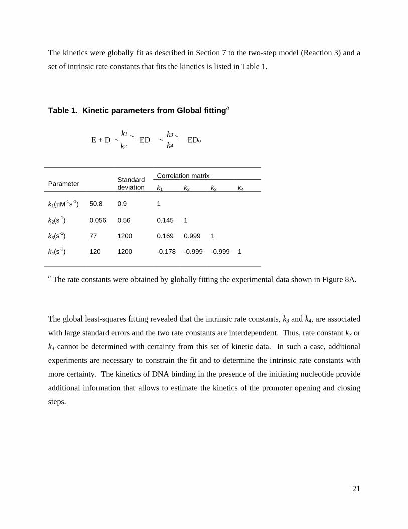
The kinetics were globally fit as described in Section 7 to the two-step model (Reaction 3) and a
set of intrinsic rate constants that fits the kinetics is listed in Table 1.
Table 1. Kinetic parameters from Global fittinga
Correlation matrixParameter Standard
deviation k1 k2 k3 k4
k1(µM-1s-1) 50.8 0.9 1
k2(s-1) 0.056 0.56 0.145 1
k3(s-1) 77 1200 0.169 0.999 1
k4(s-1) 120 1200 -0.178 -0.999 -0.999 1
a The rate constants were obtained by globally fitting the experimental data shown in Figure 8A.
The global least-squares fitting revealed that the intrinsic rate constants, k3 and k4, are associated
with large standard errors and the two rate constants are interdependent. Thus, rate constant k3 or
k4 cannot be determined with certainty from this set of kinetic data. In such a case, additional
experiments are necessary to constrain the fit and to determine the intrinsic rate constants with
more certainty. The kinetics of DNA binding in the presence of the initiating nucleotide provide
additional information that allows to estimate the kinetics of the promoter opening and closing
steps.
E + D ED EDok1
k2
k3
k4

22
4.4 DNA binding in the presence of initiating GTP
The initiation start sequence of T7 consensus promoter is (+1)GGG, hence GTP is the initiating
nucleotide. The kinetics of DNA binding were measured in the presence of the initiating
nucleotide analog, 3'-dGTP that lacks the 3'-OH group and hence the first phosphodiester bond
formation step cannot occur. The use of 3'-dGTP allows us to examine steps up to GTP binding
and induced conformational changes without the complexity of RNA synthesis (36). T7 RNAP
premixed with increasing concentration of 3'-dGTP was rapidly mixed with 2-AP modified
dsDNA. The time-dependent increase in fluorescence of 2-AP modified DNA was measured at
various 3'-dGTP concentrations (Figure 9A). Single exponential kinetics were observed whose
rates decreased with increasing [3'-dGTP] (Figure 9B). The fluorescence change or amplitude
on the other hand increased with increasing [3'-dGTP] (Figure 9B).
Figure 9: (A) Stopped-flow kinetics of 40 bp 2-AP DNA binding to T7 RNAP in the presence of theinitiating nucleotide, 3'-dGTP. A solution of T7 RNAP (1.0 µM final) and 3’-dGTP (varyingconcentrations) was mixed with a constant amount of -4T 2-AP DNA (0.15 µM final). The fluorescenceincrease was monitored (as in Figure 6B) and kinetic traces were collected on a log-time axis as shown(dots). The traces best fit to a single exponential equation (solid lines) to provide the observed rates andamplitudes. (B) The observed rates (white circles) and amplitudes (black circles) are plotted as a functionof [3’-dGTP]. The rate plot fits to Eqn. 8, which provided k = 83 ± 4 s-1, Kd,3’-dGTP = 111 ± 21 µM, and y0= 16 ± 3 s-1. The amplitude plot fits to the hyperbolic equation with K1/2 = 588 ± 97 µM.
[3'-dGTP] ( M)µ0 250 500 750 1000
0
25
50
75
100
0.0
0.2
0.4
0.6
0.8
1.0
Time (ms)10 100
2.0
2.4
2.8
3.2[3'-dGTP]1000 µM600 µM400 µM300 µM200 µM150 µM100 µM50 µM
AmplitudeRate
A B
Fluo
resc
ence
(> 3
60 n
m)
Obs
erve
d ra
te (s
)-1
Am
plitu
de

23
The above dependencies of rate and amplitude with increasing 3'-dGTP concentration is
characteristic of a mechanism where steps of DNA binding and promoter opening precede 3'-
dGTP binding as shown in Reaction 4.
Reaction 4.
If we assume that E+D to ED conversion is a fast step relative to the rate of ED to EDo
conversion, and nucleotide binding is a rapid equilibrium step, then the 3'-dGTP rate dependency
can be fit to Eqn. 8 (37).
]'3[0
'3,
'3,
dGTPKKA
ykdGTPd
dGTPdobs −+
×+=
−
− (Eqn. 8)
The fit provided Kd,3'-dGTP of 110 µM, which is approximately equal to the equilibrium
dissociation constant of the 3'-dGTP binding step, y0 of 16 s-1, which is approximately equal to
k3, and A of 80 s-1, which is approximately equal to k4 of Reaction 4. An interesting result from
these experiments is that the dissociation of EDo is about 5 times faster than its formation.
The increase in fluorescence amplitude with increasing [3'-dGTP] was fit to a hyperbola (Eqn. 9)
that provided an observed Kd of 3'-dGTP of 588 µM. The apparent Kd of 3'-dGTP is weaker and
this is consistent with Reaction 4, where ED to EDo conversion step with an unfavorable
equilibrium constant (k3/k4) precede the nucleotide binding step. The apparent Kd of 3’-dGTP =
Kd,3'-dGTP (1+1/K), where Kd,3'-dGTP is the intrinsic Kd of 3’-dGTP and K is the equilibrium
constant for the formation of EDo. If Kd,3'-dGTP is 110 µM and observed Kd,3'-dGTP is 588 µM, then
the calculated K = 0.23, which is approximately equal to k3/k4 equal to 16 s-1/80 s-1 = 0.2. To
determine more accurately the values of the intrinsic rate constants without any assumptions
involved in deriving the explicit Eqn. 8, the kinetic data from two sets of experiments (shown in
Figures 8A and 9A) were globally fit to the model in Reaction 4, similar to the procedure
described in Section 7, and the derived intrinsic rate constants are shown in Table 2.
E + D ED EDo EDoG3’-dGTPk1
k2
k3
k4 Kd,3’-dGTP

24
Table 2. Kinetic parameters from Global fitting
Correlation matrixParameter Standard
deviation k1 k2 k3 k4 Kd,3'-dGTP
k1 (µM-1s-1) 201.8 3.5 1
k2a (s-1) 7.75 NA
k3 (s-1) 16.12 0.07 -0.498 1
k4 (s-1) 141.7 0.7 -0.374 0.935 1
Kd,3'-dGTP (µM) 55.7 0.2 -0.132 -0.135 -0.256 1
a The kinetic data shown in Figures 8A and 9A were globally fit using a procedure similar to thatdescribed in Section 7. Fitting was constrained by fixing k2 = k1 * Kd,overall *(1 + k3/k4*(1 + k5*[3’-dGTP]/k6)). The Kd,overall was measured as 0.018 µM at [3’-dGTP] = 500 µM using fluorescentequilibrium titrations. Nonlinear least-squares global fitting routine was carried out using randomlychosen starting parameters, at least 33 times. The fitting converged to one set of parameters that providedthe best global fit, as judged by the sum of squared residuals. The standard deviation and the correlationmatrix for the fitted rate constants were obtained using the Jacobian calculated from the least-squaresfitting.
There are several interesting features revealed from the mechanism obtained by global fitting.
The derived rate constants reveal that T7 RNAP binds the dsDNA promoter to form a closed
complex ED with a bimolecular rate constant 200 µM-1s-1, which is a fast rate close to diffusion-
limited and similar to that observed with the p-dsDNA promoter. The closed complex
dissociates at a relatively slow rate of 7 s-1 and isomerizes to EDo with a rate constant 16 s-1. The
EDo is not kinetically stable and it reverses back to ED with a faster rate constant close to 140 s-1.
Thus, the ED to EDo conversion occurs with an unfavorable equilibrium constant, K2 of 0.11.
The mechanism also indicates that initiating NTP binds to EDo with a Kd close to 55 µM. Below
(Section 5) we describe an experiment that provided the cumulative Kd of +1 and +2 GTP, which
is at least 5 times weaker than the estimated Kd of +2 GTP of 100 µM. The intrinsic Kd of 3'-
E + D ED EDo EDoG3’-dGTPk1
k2
k3
k4 Kd,3’-dGTP
25
dGTP (50 µM) obtained from data fitting is close in value to the Kd of the +2 GTP, hence it
appears that open complex formation is driven by the binding of GTP that base-pairs with the
template at +2 position (36).
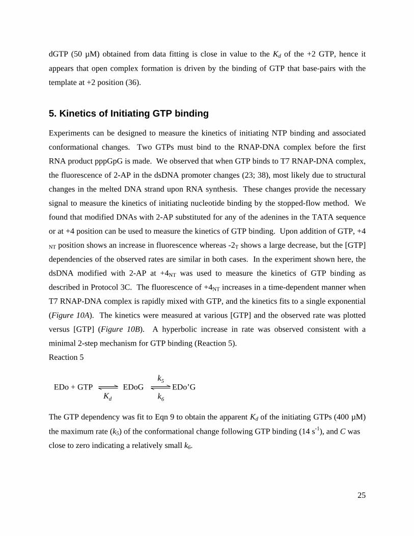
5. Kinetics of Initiating GTP binding
Experiments can be designed to measure the kinetics of initiating NTP binding and associated
conformational changes. Two GTPs must bind to the RNAP-DNA complex before the first
RNA product pppGpG is made. We observed that when GTP binds to T7 RNAP-DNA complex,
the fluorescence of 2-AP in the dsDNA promoter changes (23; 38), most likely due to structural
changes in the melted DNA strand upon RNA synthesis. These changes provide the necessary
signal to measure the kinetics of initiating nucleotide binding by the stopped-flow method. We
found that modified DNAs with 2-AP substituted for any of the adenines in the TATA sequence
or at +4 position can be used to measure the kinetics of GTP binding. Upon addition of GTP, +4
NT position shows an increase in fluorescence whereas -2T shows a large decrease, but the [GTP]
dependencies of the observed rates are similar in both cases. In the experiment shown here, the
dsDNA modified with 2-AP at +4NT was used to measure the kinetics of GTP binding as
described in Protocol 3C. The fluorescence of +4NT increases in a time-dependent manner when
T7 RNAP-DNA complex is rapidly mixed with GTP, and the kinetics fits to a single exponential
(Figure 10A). The kinetics were measured at various [GTP] and the observed rate was plotted
versus [GTP] (Figure 10B). A hyperbolic increase in rate was observed consistent with a
minimal 2-step mechanism for GTP binding (Reaction 5).
Reaction 5
The GTP dependency was fit to Eqn 9 to obtain the apparent Kd of the initiating GTPs (400 µM)
the maximum rate (k5) of the conformational change following GTP binding (14 s-1), and C was
close to zero indicating a relatively small k6.
EDo + GTP EDoG EDo’Gk5
k6Kd

26
Figure 10: Stopped-flow kinetics of GTP binding to T7 RNAP-DNA complex. (A) T7 RNAP-DNAcomplex (+4NT 2-AP DNA, 0.15 µM final concentration, and T7 RNAP, 0.45 µM final) was mixed withGTP and the fluorescence increase was monitored over time in two time windows (dots). Arepresentative trace at 2.5 mM GTP concentration is shown. The data were fit to Eqn. 4 (solid line) toobtain the observed rates. (B) The observed rate is plotted against [GTP] (white circles). The data werefit to the hyperbolic Eqn. 9, which provided a cumulative Kd of GTPs = 400 ± 70 µM and a maximum rateof the GTP inducted conformation change (B) = 14.2 ± 0.8 s-1. The GTP binding kinetics were measuredin the presence of GMP (600 µM final), and the [GTP] dependence data in the presence of GMP (blackcircles) were fit to the hyperbolic Eqn. 9 that provided the Kd of +2 GTP = 80 ± 10 µM, and a rate of GTPinduced conformational change (B) = 14.5 ± 0.4 s-1.
(Eqn. 9)
The same experiment was carried out in the presence of a constant amount of GMP to determine
the relative Kd values of +1 and +2 GTPs. It has been shown that T7 RNAP can initiate very
efficiently with GMP, implying that the +1 position can bind GMP. However, the binding of
GMP alone does not result in fluorescence changes. In the presence of saturating concentration
of GMP, The GTP binding kinetics can provide the Kd of +2 GTP. In the presence of 600 µM
GMP, the observed Kd of GTP is 80 µM (Figure 10B). The observed Kd of GTP in the presence
of GMP provides the upper limit of the Kd of +2 GTP (80 µM) and indicates that +2 GTP binds
tighter than the +1 GTP, whose Kd is estimated to be > 400 µM (measured GTP Kd in the
absence of GMP).
[GTP] ( M)µ0 500 1000 1500 2000 2500
0
5
10
15
B - GMP+ GMP
A B
1.0 1.5Time (s)
0.1 0.3 0.5
5.85
5.90
5.95Fl
uore
scen
ce (>
360
nm
)
Obs
erve
d ra
te (s
)-1
CGTPK
GTPkk
dobs +
+×=
][][5
27
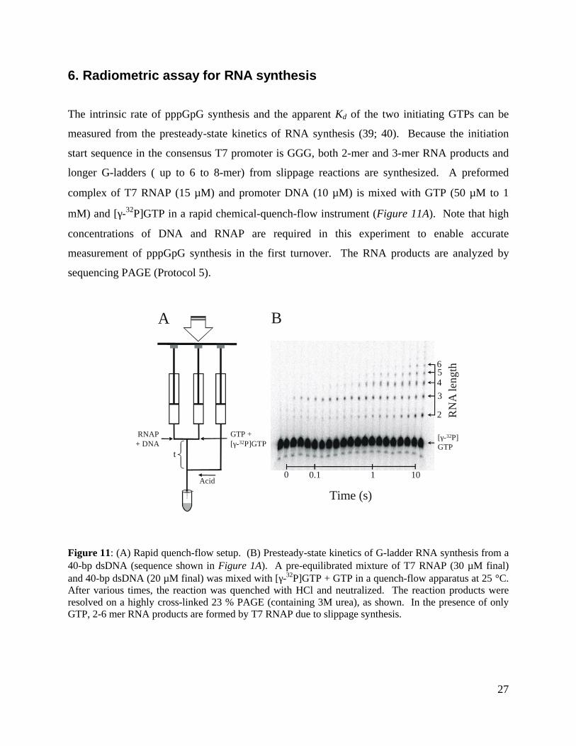
6. Radiometric assay for RNA synthesis
The intrinsic rate of pppGpG synthesis and the apparent Kd of the two initiating GTPs can be
measured from the presteady-state kinetics of RNA synthesis (39; 40). Because the initiation
start sequence in the consensus T7 promoter is GGG, both 2-mer and 3-mer RNA products and
longer G-ladders ( up to 6 to 8-mer) from slippage reactions are synthesized. A preformed
complex of T7 RNAP (15 µM) and promoter DNA (10 µM) is mixed with GTP (50 µM to 1
mM) and [γ-32P]GTP in a rapid chemical-quench-flow instrument (Figure 11A). Note that high
concentrations of DNA and RNAP are required in this experiment to enable accurate
measurement of pppGpG synthesis in the first turnover. The RNA products are analyzed by
sequencing PAGE (Protocol 5).
Figure 11: (A) Rapid quench-flow setup. (B) Presteady-state kinetics of G-ladder RNA synthesis from a40-bp dsDNA (sequence shown in Figure 1A). A pre-equilibrated mixture of T7 RNAP (30 µM final)and 40-bp dsDNA (20 µM final) was mixed with [γ-32P]GTP + GTP in a quench-flow apparatus at 25 °C.After various times, the reaction was quenched with HCl and neutralized. The reaction products wereresolved on a highly cross-linked 23 % PAGE (containing 3M urea), as shown. In the presence of onlyGTP, 2-6 mer RNA products are formed by T7 RNAP due to slippage synthesis.
t
RNAP + DNA
GTP +[γ-32P]GTP
Acid
A B
0 0.1 1 10
Time (s)
[γ-32P]GTP
2
3456
RN
A le
ngth

28
Protocol 5. Presteady-state kinetics of pppGpG synthesis by the rapid chemical-
quench-flow methoda
Equipment and reagents
• Quench-flow instrument (KinTek Corp., Austin, TX), attached to a circulating water bath
• Bio-Rad sequencing gel apparatus (0.25 mm thick spacers and comb)
• Phosphor screen, PhosphorImager instrument (Molecular Dynamics),ImageQuaNT program for
quantitative data analysis
• 1.5 ml eppendorf tubes having lids punched with a hole slightly larger than the diameter of the exit
line tubing
• 23 % (w/v) polyacrylamide-3% bis sequencing gel containing 3 M urea
• Sequencing gel loading dye
• 40 bp dsDNA promoter (non 2-AP) and T7 RNAP
• GTP and [γ-32P]GTP
• 1N HCl, neutralization base mixture (1M NaOH + 0.25M Tris base), and Chloroform
• High salt 1x reaction buffer: Same as in Protocol 2, except Na-acetate = 100 mM
• Low salt 1x reaction buffer: Same as in Protocol 2, but with no Na-acetate
Method
1. Prepare sequencing gel and pre-run at 110W (55 °C) while collecting the time course on the quench-
flow instrument.
2. Set the temperature of the water bath connected to the quench-flow apparatus to 25 °C, fill the two
drive syringes A and B with water, and the third drive syringe C with 1 N HCl.
3. Prepare a solution of T7 RNAP (30 µM) and 40 bp dsDNA (20 µM) in high salt 1x reaction buffer and
allow to equilibrate.
4. Load equilibrated RNAP-DNA solution (25 µl approx.) in one sample loopb (see set up in Figure 11)

29
and an equal volume of a selected concentration of the GTP solution containing [γ-32P]GTP (in low
salt 1x reaction buffer) in second sample loopb.
5. Mix and quench the reaction after a set time, and collect the sample in a 1.5 ml eppendorf tube under
the exit line.
6. Add 100 µl Chloroform, vortex mix and centrifuge.
7. Within 1 min, neutralize (test on a pH strip) with appropriate volume of the neutralization base
mixture.
8. Rinse the sample loading loops, reaction loop and exit line first with water and then with MeOH.
9. Repeat steps 4 - 8, varying the reaction time in step 5.
10. Perform a control experiment - repeat steps 4 - 8 without loading GTP in step 4. Add GTP after step
6. This serves as a blank for measurement of the background in the experiment.
11. Mix 10 µl of the neutralized reaction solution (from aqueous layer) with 2 µl of the sequencing dye.
12. Load 10 µl of each sample on the gel and run at 110W (55 °C) for appox. 3 h.
13. Expose the gel to phosphor screen (duration of exposure will vary depending on the radioactivity
present), scan the exposed screen using PhosphorImager.
14. Quantitate the substrate and RNA products using ImageQuaNT software. If the counts exceed the
range of sensitivity, re-expose the screen for a shorter duration and scan again (step 13).
15. Calculate the µM amount of RNA product at each time point = [GTP] µM x (counts for total RNA/
counts for GTP + counts for total RNA). Plot total RNA product versus time and fit the data to Eqn 10.
16. Perform the experiment using various concentrations of GTP, and plot burst rate versus [GTP] as
shown in Figure 12B.
a For a detailed discussion on the method, see reference (3)
b Because equal volumes of two solutions are mixed, the loading solutions are used at double the
concentrations studied in the experiment.
_____________________________________________________________________________

30
A typical time course of pppGpG and longer G-ladder synthesis is shown in Figure 11B. The
plot of total RNA versus time is nonlinear and a presteady-state burst of G-ladder synthesis is
observed (Figure 12A). The burst kinetics are fit to Eqn. 10.
CtbkteAy +×+
−−×= 1 (Eqn. 10)
Where A is burst amplitude, k is burst rate, b is steady-state rate, and C is y-intercept. The burst
kinetics indicates that the synthesis of 2-mer and 3-mer RNA is rapid on the RNAP active site.
The steady-state rate (b) of abortive RNA synthesis is limited either by the rate of product
dissociation or the rate of RNAP recycling on the promoter. The steady-state rate constant is
therefore a complex parameter that cannot be interpreted meaningfully in terms of the
mechanism of transcription initiation. The burst amplitude (A) provides the concentration of
active T7 RNAP-DNA complex, and the burst rate (k) the synthesis rate of 2-mer and 3-mer
RNA. It is clear from Figure 11B that 2-mer RNA does not accumulate in the presteady-state
time scale. Thus, 2-mer to 3-mer conversion is fast relative to the rate of 2-mer formation.
Figure 12: Presteady-state kinetics of RNA synthesis during transcription initiation. (A) A pre-equilibrated mixture of T7 RNAP-DNA was mixed with increasing concentrations of GTP (+ [γ-32P]GTP)in a quench-flow apparatus, as in Figure 11. Time courses of total RNA synthesis at various GTPconcentrations are shown. The solid lines are fit to the burst equation (Eqn. 10). (B) The burst rates areplotted as a function of [GTP] (circles). The plot was fit to the hyperbolic equation (Eqn. 9) that providesa cumulative Kd of initiating GTPs = 330 ± 90 µM, and a maximum rate of the burst phase = 7.8 ± 0.7 s-1.
Time (s)0.0 0.5 1.0 1.5 2.0
0
10
20
30
[GTP] ( M)µ0 500 1000 1500 2000
0
2
4
6
A B
300 µM600 µM900 µM1500 µM
100 µM150 µM200 µM[GTP]To
tal R
NA
(M
)µ
Bur
st R
ate
(s)
-1

31
Hence, the burst rate provides an estimate of 2-mer formation, which is limited either by the rate
of first phosphodiester bond formation reaction or preceding step/s.
The presteady-state kinetics is measured at various [GTP], and the observed burst rate is plotted
versus [GTP] (Figure 12B). The burst rate increases in a hyperbolic manner with increasing
[GTP], which was fit to Eqn. 9 to obtain the apparent Kd of initiating GTPs (cumulative Kd of +1
and +2 GTP) and the observed maximum rate of pppGpG synthesis. The Kd of initiating GTPs
from this radiometric assay (330 ± 90 µM) is very close to the GTP Kd obtained from
fluorescence stopped-flow experiments described above. Similarly, the rate of pppGpG
synthesis (7.8 ± 0.7 s-1) is about two times slower than the rate of the conformational change
upon GTP binding obtained from the stopped-flow experiments (Section 5). Thus, combination
of radiometric rapid chemical-quench-flow and fluorescence stopped-flow methods provide
values of initiating GTP Kd , the rate of conformational change and pppGpG synthesis rate.
The entire description of the transcription initiation pathway can be obtained from the
combination of stopped-flow fluorescence and radiometric rapid quench-flow methods. The goal
of elucidating each step in the pathway is also to understand how transcription is regulated
intrinsically by promoter sequence and by accessory factors such as transcription factors and
small ligands that regulate transcription. The process involves measuring the intrinsic rate
constants of the initiation pathway with each promoter variant and in the presence of the effector,
and then comparing the constants to that of the consensus promoter to identify the microscopic
steps that are affected. This information should be combined with available structural
information to obtain a complete understanding of the structure and dynamics of the enzymatic
reaction and its regulation.
7. Data Simulation and Fitting
Transient-state kinetic experiments are designed to monitor the accumulation and decay of the
reacting species. The observed rates that are obtained from these types of experiments allow the
investigator to propose a mechanism of the reaction. The next steps are a) verify that the
proposed mechanism accounts for the observed phenomena, b) determine the intrinsic rate
32
constants for each step of the mechanism, and c) test for alternative mechanisms. These tasks
can be accomplished by computer curve fitting of all the available experimental data.
Computer curve fitting can be a fairly complicated task involving repeated simulation of the
reaction mechanism trying to find a set of rate constants that fit the experimental data the best. A
number of software packages are available for this purpose. However, quite often the flexibility
and performance of these packages is not sufficient if the reaction mechanism is complicated, or
different types of experiments need to be globally fit, or the number of fitting parameters is large.
In such cases specific instructions for simulation and fitting can be programmed in MATLAB
(The MathWorks, Inc., Natick, MA) that simplifies this task by providing functions for data
manipulation, simulation and curve fitting.
In this section we discuss how to perform simulation and global fitting of enzyme kinetic data in
the MATLAB computing environment. We also show how to calculate the basic statistics of the
parameters obtained from fitting and how to deal with the ‘local minimum’ problem in curve
fitting. The software, MATLAB and the Optimization Toolbox, can be downloaded for a 30 day
trial period from www.mathworks.com. Only a very basic knowledge of MATLAB is needed to
follow our examples. A brief inspection of "Getting Started with MATLAB" or "Learning
MATLAB" available for download should be sufficient. Attention should be paid to chapters
“Getting started” and “Programming with MATLAB”. To illustrate the process of data fitting
and analysis we take the experiment described in Section 4.3 and use Reaction 3 as the model for
T7 RNAP interaction with dsDNA.
7.1 Model building and simulation
Enzyme model is built in the form of a reaction scheme (for example, Reaction 3) that shows all
reacting species and rates of their interconversion. Simulation involves calculation of the
concentrations of the reacting species and the expected signal (Figures 6B, 8A) as a function of
time. This is accomplished by solving a system of ordinary differential equations (ODE)
corresponding to that mechanism. Only the simplest ODE can be solved analytically, therefore
numerical iteration methods are employed for simulation.

33
Several software packages are available to perform enzyme kinetic simulation. They vary by
their user interface, performance, and flexibility. A user friendly program, KINSIM, allows the
mechanism to be entered in the form of a reaction scheme (41-43). Scientist (MicroMath
Scientific Software, Salt Lake City, UT) is aimed for broader range of simulation and data fitting
problems, and it automatically solves implicit equations and systems of ODE with a minimal
amount of programming. A more flexible software package MATLAB provides its own
environment, programming language, and a collection of routines. Reaction mechanisms can be
programmed in MATLAB and simulated using one of its built-in ODE solvers. Even though
MATLAB requires a little bit more programming, simulation and fitting tasks are executed
several times faster in MATLAB than in Scientist. One main advantage of MATLAB is that it
provides a greater flexibility in programming complex reaction mechanisms.
The example discussed here is relatively simple. The experiment consists of mixing a known
concentration of T7 RNAP (E) with 2-AP DNA (D) in a stopped-flow apparatus (Figure 6A) and
fluorescence signal is measured as a function of time (Figure 8A) (Section 4.3). The experiment
is repeated with different concentrations of E. The experimental data (Figure 8) indicated that
T7 RNAP binds to a dsDNA promoter in a two-step mechanism (Reaction 3), involving a closed
complex intermediate (ED) followed by an isomerization step of dsDNA opening to form an
open complex (EDo), which has a higher fluorescence coefficient.
EDok
kED
k
kDE ←
→ ← →
+4
3
2
1
This reaction scheme can be described by a system of ODEs:
EDokEDkdt
dEDo
EDkEDkEDokDEkdt
dED
DEkEDkdtdD
DEkEDkdtdE
×−×=
×−×−×+××=
××−×=
××−×=
43
3241
12
12

34
With known initial concentrations of E and D and rate constants (k1 through k4), the system of
differential equations can be solved to yield a time course of all the reacting species. MATLAB
provides several ODE solver functions that use different numerical methods. We found that the
ODE solver ode15s produces the best results for our enzyme kinetics problems. This solver is
designed for ODEs, whose solutions make large changes over a small time interval (stiff ODE).
The system of ODE is defined in a mechanism M-file used by the ODE solver. The function
mech (Protocol 6) accepts a vector of concentrations, y from the ODE solver and calculates a
vector of differentials, dy/dt.
To improve the ODE solver performance, function mech was also programmed to calculate
Jacobian Df(y) of the ODE. Although in the case discussed here, only a small increase in
performance was observed.
( )
( ) ( )
( ) ( )
∂∂
∂∂
∂∂
∂∂
=
n
nn
n
yf
yf
yf
yf
Dyy
yy
yf
L
MOM
L
1
1
1
1
Where y is a vector of concentrations of n reacting species, and f(y) is its differential dy/dt.
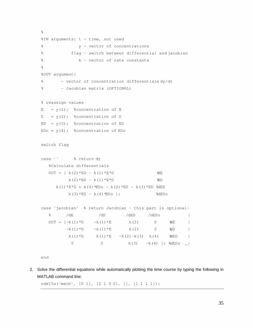
Protocol 6. Simulation of a kinetic mechanism
This protocol requires MATLAB version 5.3 installed on your computer.
1. Create an M-file mech.m containing the following function. Make sure mech.m is in the directory
path.
function OUT = mech(t, y, flag, k)
% dy = mech(t, y, flag, k)
% Differential equations for the following mechanism
% k1> k3>
% E + D == ED == EDo
% <k2 <k4
%
%This function is used by the ODE solver
35
%
%IN arguments: t - time, not used
% y - vector of concentrations
% flag - switch between differential and jacobian
% k - vector of rate constants
%
%OUT argument:
% - vector of concentration differentials dy/dt
% - Jacobian matrix (OPTIONAL)
% reassign values
E = y(1); %concentration of E
D = y(2); %concentration of D
ED = y(3); %concentration of ED
EDo = y(4); %concentration of EDo
switch flag
case '' % return dy
%Calculate differentials
OUT = [ k(2)*ED - k(1)*E*D %dE
k(2)*ED - k(1)*E*D %dD
k(1)*E*D + k(4)*EDo - k(2)*ED - k(3)*ED %dED
k(3)*ED - k(4)*EDo ]; %dEDo
case 'jacobian' % return Jacobian – this part is optional-
% /dE /dD /dED /dEDo |
OUT = [-k(1)*D -k(1)*E k(2) 0 %dE |
-k(1)*D -k(1)*E k(2) 0 %dD |
k(1)*D k(1)*E -k(2)-k(3) k(4) %dED |
0 0 k(3) -k(4) ]; %dEDo _|
end
2. Solve the differential equations while automatically plotting the time course by typing the following in
MATLAB command line:
ode15s('mech', [0 1], [2 1 0 0], [], [1 1 1 1]);

36
As shown in Protocol 6, a single time course can be simulated from the MATLAB command
line. However, it is desirable to simulate all the time courses collected at various concentrations
of E and plot the resulting fluorescence along with the experimental data. We first discuss how
to enter the experimental data into MATLAB (Protocol 7).
A small set of data (a column of up to a few hundred numbers) can be pasted directly into
MATLAB command line after 'var = [' statement, where var is a name of a variable, and
followed by a square bracket and a semicolon ']. For a large or multicolumn set of data it is more
convenient to create an M-file. The experimental data may consist of several time courses, but it
is convenient to treat it as a single vector, because storing the data in a two-dimensional array is
only possible for time courses with equal number of data points. Therefore, time and the
corresponding fluorescence values from all the time courses should be placed in two columns as
described in Protocol 7.
Protocol 7. Entering data into MATLAB
This protocol requires MATLAB version 5.3 installed on your computer. We assume that your data is
already in a spreadsheet format with unique values of time in ascending order within each time
course.
1. Stagger all t versus f pairs from all time courses into two columns of a spreadsheet.
2. Copy the column t into the clipboard, switch to MATLAB Editor/Debugger, paste the numbers into a
blank document, and edit the first and the last lines so that the document has the following form:
t=[ t(1)
t(2)
...
t(n) ];
Save the document as time.m. Now load the values of time into the memory as a vector t by typing in
the MATLAB command line:
time
3. In a similar manner create a file flu.m that loads all fluorescence values into vector fx. Make sure
vectors t and fx have same dimensions.

37
4. Now create array C containing experimental conditions. It contains as many rows as the number of
time courses. The first column contains starting concentrations of T7 RNAP (E). The second column
contains starting concentrations of 2-AP DNA (D). The third column, which refers to vectors t and fx
contains the row number for the last time point in each time course. Type or paste the values of array
C into MATLAB command line, or load the array C from an M-file as before. Generate the third
column of the array by executing the following MATLAB command:
C(:,end+1) = find(t-[t(2:end); 0] > 0)
The M-file simulate.m shown in Protocol 8 calculates the expected fluorescence for multiple
time courses in the following manner. Each time course is simulated, and the concentration of
EDo is converted into fluorescence, F = F0 + EDo × fEDo. Where F0 is the initial fluorescence (at
t = 0) of the species in the reaction mixture, and fEDo is a fluorescence coefficient. The
fluorescence parameters are affected by inner filter effect and the voltage on the PMT; therefore,
independent values of F0 and fEDo are associated with each time course. Finally, the simulated
fluorescence values for all time courses are arranged in one column. Note that the option
‘Jacobian’, although implemented in our example, is not necessary. It may significantly improve
the performance of the ODE solver in case of a stiffer reaction mechanism, but may be difficult
to implement. Incorrectly programmed Jacobian will reduce the performance of the solver. The
vector param, that stores rate constants and fluorescence coefficients, can be changed manually
to bring the simulation closer to the experimental data. Function PlotDS (Protocol 8) plots
experimental and simulated data on a semilog plot.
Protocol 8. Simulation and plotting of multiple time courses
This protocol requires MATLAB version 5.3 installed on your computer, file mech.m (Protocol 6)
located in the path, and variables t, fx, and C (Protocol 7) stored in the memory.
1. Create an M-file simulate.m .
function fsim = simulate(param, t, C)
%fsim = simulate(param, t, C)
%simulates many time courses
%
%IN ARGUMENTS:
%param - vector of parameters
% [k(1) )

38
% ... > rate constants
% k(r) )
% f0(1) trace 1)
% ... ... > starting fluorescence
% f0(n) trace n)
% fEDo(1) trace 1 )
% ... ... > fluorescence coefficient
% fEDo(n)]trace n )
%
% t - vector of times for all experiments
%
% matrix C = | E(1) D(1) tend(1) | trace 1
% | ... ... ... | ...
% | E(n) D(n) tend(n) | trace n
%
% OUT ARGUMENTS fsim - vector of fluorescence values
% for all simulated time courses
raten = 4; %number of rate constants
n = size(C, 1);%number of experiments
options = odeset('RelTol', 1e-5, 'AbsTol', 1e-7...
,'Jacobian', 'on'... %improves performance
); %disable previous line with ‘...’ if -
%the mechanism does not support these options
fsim = [ ]; %matrix of simulated fluorescence time courses
% Check input sizes
if length(param) ~= raten + n*2
disp('Wrong number of parameters!'); return;
end
if length(t) ~= C(end,end)
disp('Wrong number of times'); return;
end

39
%%%%%%%%%%%%%%%%%%%%%%%%%%%%%%%%%%%%%%%%%%%%%%%%%%%%%%%%%%%%%%%
%SIMULATE ALL TRACES
tstart = 1; %1st point of the 1st trace
for i = 1:n %trace number
tcurr = t(tstart:C(i,end)); %time vector for current trace
tstart = C(i,end) + 1; %1st point of the next trace
[tcurr, Y] = ode15s(... %call ODE solver
'mech', ... %mechanism M-file
tcurr, ... %time points
[C(i,1); C(i,2); 0; 0], ... %starting concentrations of E;D;ED;EDo
options, ... %ODE solver options
param(1:raten)); %rate constants
f = ... %fluorescence for current trace
Y(:,end) * ... %only the last species fluoresce
param(raten + n + i)... %multiply by fluorescence coefficient
+ param(raten + i); %starting fluorescence
fsim = [fsim; f]; %stagger all traces
end
2. Create a vector param containing four rate constants, starting fluorescence values (one for each time
course), and fluorescence coefficients (one for each time course).
param = [1 1 1 1 3:0.4:9 20*ones(1,16)]';
3. Simulate all the time courses simultaneously by executing the function simulate from the MATLAB
command linea.
fsim = simulate(param, t, C);
4. Create an M-file PlotDS.m that plots data and simulated points.
function PlotDS(t, fx, fsim, C)
%PlotDS(t, fx, fsim, C) - plots data and simulation
% Plots each trace of the experimental data
% on the same graph as dots
% Adds simulations as lines

40
tstart = [1; C(1 : end-1, 3) + 1]; %trace starting points
tend = C(:, 3); %trace end points
n = size(C, 1); %number of traces
scrsz = get(0,'ScreenSize'); %adjust figure size
figure('Position',[1 scrsz(4)*.05 scrsz(3)/2 scrsz(4)*0.85]);
for i = 1:n %for each trace
semilogx(t(tstart(i):tend(i)),... %plot time vs
fx(tstart(i):tend(i)),... %experimental points
'k.',... %as black dots
t(tstart(i):tend(i)),... %and time vs
fsim(tstart(i):tend(i)),... %simulated points
'r-') %as red lines
hold on %plot next on the same graph
end
hold off
5. Plot the results of the simulation by typing in MATLAB command line:
PlotDS(t, fx, fsim, C)
6. Try changing the vector param, re-simulate, and re-plot the results.
a It takes about 10 s to simulate 16 traces on Pentium III 550 MHz computer.
7.2 Data fitting
Data fitting (curve fitting) is a method of refining a scientific model. It is used to determine the
parameters when the overall form of the model is known. Technically, data fitting is an
optimization problem of finding the parameters of a function such that the values of the function
closely approximate the experimental data. The parameters producing a 'good fit' are considered
to be close to the 'true parameters' assuming that the independent variables, time and
concentrations, are known precisely and the experimental results are randomly distributed around
their ‘true values’. The last assumption can only be made if the experimental results are not
affected by a systematic error (such as bleaching, in case of a fluorimetric experiment) and a
non-linear transformation has not been applied to them.
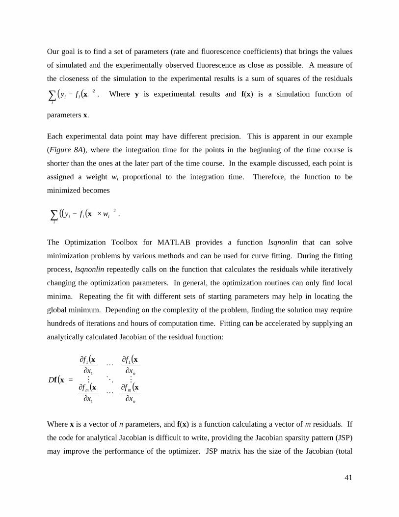
41
Our goal is to find a set of parameters (rate and fluorescence coefficients) that brings the values
of simulated and the experimentally observed fluorescence as close as possible. A measure of
the closeness of the simulation to the experimental results is a sum of squares of the residuals
( )( )∑ −i
ii fy 2x . Where y is experimental results and f(x) is a simulation function of
parameters x.
Each experimental data point may have different precision. This is apparent in our example
(Figure 8A), where the integration time for the points in the beginning of the time course is
shorter than the ones at the later part of the time course. In the example discussed, each point is
assigned a weight wi proportional to the integration time. Therefore, the function to be
minimized becomes
( )( )( )∑ ×−i
iii wfy 2x .
The Optimization Toolbox for MATLAB provides a function lsqnonlin that can solve
minimization problems by various methods and can be used for curve fitting. During the fitting
process, lsqnonlin repeatedly calls on the function that calculates the residuals while iteratively
changing the optimization parameters. In general, the optimization routines can only find local
minima. Repeating the fit with different sets of starting parameters may help in locating the
global minimum. Depending on the complexity of the problem, finding the solution may require
hundreds of iterations and hours of computation time. Fitting can be accelerated by supplying an
analytically calculated Jacobian of the residual function:
( )
( ) ( )
( ) ( )
∂∂
∂∂
∂∂
∂∂
=
n
mm
n
xf
xf
xf
xf
Dxx
xx
xf
L
MOM
L
1
1
1
1
Where x is a vector of n parameters, and f(x) is a function calculating a vector of m residuals. If
the code for analytical Jacobian is difficult to write, providing the Jacobian sparsity pattern (JSP)
may improve the performance of the optimizer. JSP matrix has the size of the Jacobian (total
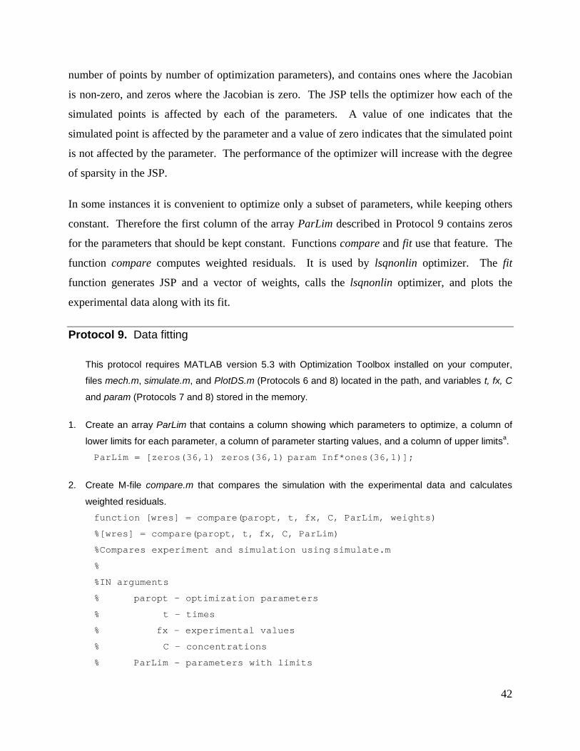
42
number of points by number of optimization parameters), and contains ones where the Jacobian
is non-zero, and zeros where the Jacobian is zero. The JSP tells the optimizer how each of the
simulated points is affected by each of the parameters. A value of one indicates that the
simulated point is affected by the parameter and a value of zero indicates that the simulated point
is not affected by the parameter. The performance of the optimizer will increase with the degree
of sparsity in the JSP.
In some instances it is convenient to optimize only a subset of parameters, while keeping others
constant. Therefore the first column of the array ParLim described in Protocol 9 contains zeros
for the parameters that should be kept constant. Functions compare and fit use that feature. The
function compare computes weighted residuals. It is used by lsqnonlin optimizer. The fit
function generates JSP and a vector of weights, calls the lsqnonlin optimizer, and plots the
experimental data along with its fit.
Protocol 9. Data fitting
This protocol requires MATLAB version 5.3 with Optimization Toolbox installed on your computer,
files mech.m, simulate.m, and PlotDS.m (Protocols 6 and 8) located in the path, and variables t, fx, C
and param (Protocols 7 and 8) stored in the memory.
1. Create an array ParLim that contains a column showing which parameters to optimize, a column of
lower limits for each parameter, a column of parameter starting values, and a column of upper limitsa.
ParLim = [zeros(36,1) zeros(36,1) param Inf*ones(36,1)];
2. Create M-file compare.m that compares the simulation with the experimental data and calculates
weighted residuals.
function [wres] = compare(paropt, t, fx, C, ParLim, weights)
%[wres] = compare(paropt, t, fx, C, ParLim)
%Compares experiment and simulation using simulate.m
%
%IN arguments
% paropt - optimization parameters
% t - times
% fx - experimental values
% C - concentrations
% ParLim - parameters with limits

43
% weights - significance of each experimental point
%
%OUT arguments
% wres - weighted residuals
optimize = find(ParLim(:,1)); %vector of parameters to optimize
if length(optimize) %there are parameters to optimize
ParLim(optimize, 3) = paropt; %put optimized parameters back
end
wres = (fx - simulate(ParLim(:,3), t, C)) .* weights;
3. Create M-file fit.m that minimizes the residuals by finding the optimal set of parameters.
function [ParLim, residual, resnorm, Jac] = fit(t, fx, C, ParLim)
%[ParLim, residual, resnorm, Jac] = fit(t, fx, C, ParLim)
%Minimizes function compare.m
%
% IN arguments:
% t - vector of time values
% fx - vector of experimental fluorescence values
% matrix C = | E(1) D(1) tend(1) | trace 1
% | ... ... ... | ...
% | E(n) D(n) tend(n) | trace n
%
% optim LoLim Start HiLim
%ParLim| 1/0 ... k(1) ...| rate constants
% | 1/0 ... ... ...|
% | 1/0 ... k(r) ...|
% | 1/0 ... f0(1) ...| initial fluorescence values
% | 1/0 ... ... ...|
% | 1/0 ... f0(n) ...|
% | 1/0 ... fDo(1) ...| EDo fluorescence coefficient
% | 1/0 ... ... ...|
% | 1/0 ... fDo(n) ...|
% parameters with 0 in 1st column are fixed
%
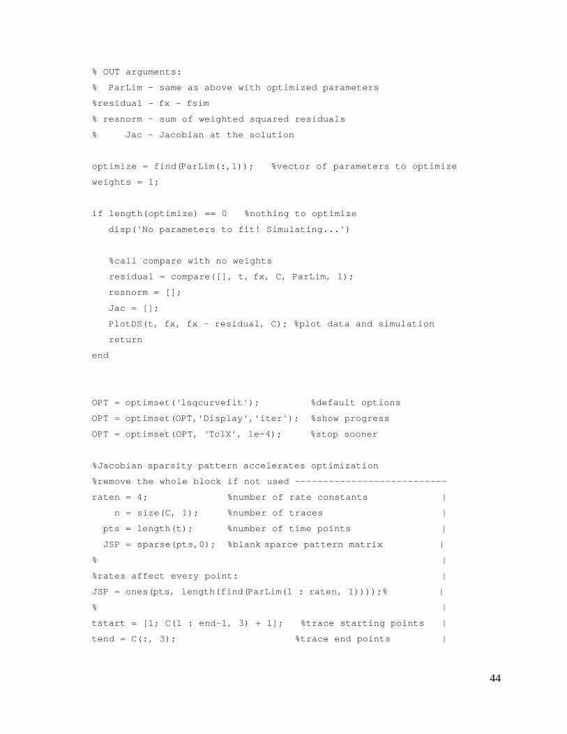
44
% OUT arguments:
% ParLim - same as above with optimized parameters
%residual - fx - fsim
% resnorm - sum of weighted squared residuals
% Jac - Jacobian at the solution
optimize = find(ParLim(:,1)); %vector of parameters to optimize
weights = 1;
if length(optimize) == 0 %nothing to optimize
disp('No parameters to fit! Simulating...')
%call compare with no weights
residual = compare([], t, fx, C, ParLim, 1);
resnorm = [];
Jac = [];
PlotDS(t, fx, fx - residual, C); %plot data and simulation
return
end
OPT = optimset('lsqcurvefit'); %default options
OPT = optimset(OPT,'Display','iter'); %show progress
OPT = optimset(OPT, 'TolX', 1e-4); %stop sooner
%Jacobian sparsity pattern accelerates optimization
%remove the whole block if not used ---------------------------
raten = 4; %number of rate constants |
n = size(C, 1); %number of traces |
pts = length(t); %number of time points |
JSP = sparse(pts,0); %blank sparce pattern matrix |
% |
%rates affect every point: |
JSP = ones(pts, length(find(ParLim(1 : raten, 1))));% |
% |
tstart = [1; C(1 : end-1, 3) + 1]; %trace starting points |
tend = C(:, 3); %trace end points |

45
J2=sparse(pts,0); %fluorescence coefficient part of JSP matrix |
% |
for i=1:n % |
if ParLim(raten + i, 1) %initial fluorescence is optimized |
%put 1 for each point in that trace |
JSP(tstart(i):tend(i), end+1) = 1;% |
end % |
% |
if ParLim(raten + n + i, 1)%fluorescence coefficient is optimized |
%put 1 for each point in that trace |
J2(tstart(i):tend(i), end+1) = 1;% |
end % |
end % |
JSP=[JSP, J2]; % |
OPT = optimset(OPT, 'JacobPattern',JSP); %tell optimizer |
%--------------------------------------------------------------
%calculate weights, or assume weights = 1 and remove------------
%weights are proportional to fluorescence integration time |
t1 = [0;t(1:end-1)]; %start integrations times|
weights = t - t1; %length of integration |
weights = weights + t1 .*(weights <0);%fix 1st points in traces|
weights = weights / mean(weights); %average weight is 1 |
%weights = 1; %remove weights--------------------------
% Start optimizer
[x,resnorm,wres,exitflag,output,lambda,Jac] = ...
lsqnonlin('compare',... %function to optimize
ParLim(optimize, 3),... %starting parameters
ParLim(optimize, 2),... %lower bound
ParLim(optimize, 4),... %upper bound
OPT, ... %optimization options
t, fx, C, ParLim, weights); %pass-on arguments
disp(output) %show optimization summary
ParLim(optimize, 3) = x; %put optimized parameters back

46
residual = wres ./ weights; %remove weights from residuals
PlotDS(t, fx, fx-residual, C);%plot experiment and fit
4. Call function fit by typing in the MATLAB command line.
fit(t, fx, C, ParLim);
Note that the function detects that only zeros are present in the first column of ParLim and just
performs a simulation and plotting. Change the first column of ParLim to all ones:
ParLim(:,1) = 1;
and perform the fitting with storing the results in the memory:b
[ParNew, residual, resnorm, Jac] = fit(t, fx, C, ParLim);
Check the generated graph for the quality of the fit, and note the new optimized parameters in the
third column of the array ParNew.
a make sure vector param is vertical
b the optimization took almost 50 min on 550 MHz Pentium III computer
Function NLRStat (Protocol 10) calculates the statistics for the optimized parameters based on
the Jacobian and a sum of squared residuals provided by lsqnonlin. NLRStat calculates the
standard deviation of the data, sigma2, a vector of standard errors for each parameter, stder, and
a correlation matrix, Corr. The correlation matrix shows how much parameters depend on each
other, that is, how much a small change in one parameter can compensate for a change in
another.
Protocol 10. Analysis of fitting results
This protocol requires MATLAB version 5.3 installed on your computer, and variables resnorm and
Jac, products of function fit (Protocol 9) stored in the memory.
1. Create an M-file function NLRStat.m that analyzes the statistics of the non-linear regression fitting.
function [sigma2, stder, Corr] = NLRStat(resnorm, Jac)
%[sigma2, stder, Corr, VCM] = NLRStat(resnorm, Jac)

47
% Computes nonlinear regression fit statistics
%
% resnorm - sum of squares of weighted residuals
% Jac – Jacobian at the optimization minimum
%
% sigma2 - sigma squared, error variance of the model
% stder - standard error of parameters
% Corr - correlation matrix
[dpts, fpar] = size(Jac);%number of data points and fitting parameters
if dpts <= fpar
disp('Number of data points should be greater than number of fitting
parameters.')
return
end
sigma2 = resnorm / (dpts - fpar); %standard deviation of data
VCM = full(inv(Jac' * Jac) * sigma2); %variance-covariance matrix
stder = full(sqrt(diag(VCM)));
Corr = full(VCM ./ (stder * stder'));
2. To calculate the optimization statistics call function NLRStat by typing in the MATLAB command line
[sigma2, stder, Corr, VCM] = NLRStat(resnorm, Jac)
Sometimes the optimization routine does not converge on a "good fit" to the experimental data.
This may be due to an incorrect model or the optimizer may be "trapped" in a local minimum,
which is far from the global one. Several steps can be taken to find the global minimum.
(i) Use better starting parameters,
(ii) Fit a subset of the experimental data to obtain better starting parameters,
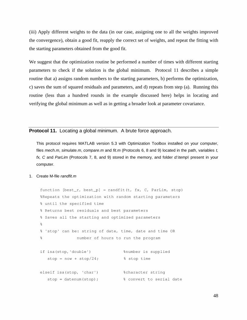
48
(iii) Apply different weights to the data (in our case, assigning one to all the weights improved
the convergence), obtain a good fit, reapply the correct set of weights, and repeat the fitting with
the starting parameters obtained from the good fit.
We suggest that the optimization routine be performed a number of times with different starting
parameters to check if the solution is the global minimum. Protocol 11 describes a simple
routine that a) assigns random numbers to the starting parameters, b) performs the optimization,
c) saves the sum of squared residuals and parameters, and d) repeats from step (a). Running this
routine (less than a hundred rounds in the example discussed here) helps in locating and
verifying the global minimum as well as in getting a broader look at parameter covariance.
Protocol 11. Locating a global minimum. A brute force approach.
This protocol requires MATLAB version 5.3 with Optimization Toolbox installed on your computer,
files mech.m, simulate.m, compare.m and fit.m (Protocols 6, 8 and 9) located in the path, variables t,
fx, C and ParLim (Protocols 7, 8, and 9) stored in the memory, and folder d:\temp\ present in your
computer.
1. Create M-file randfit.m
function [best_r, best_p] = randfit(t, fx, C, ParLim, stop)
%Repeats the optimization with random starting parameters
% until the specified time
% Returns best residuals and best parameters
% Saves all the starting and optimized parameters
%
% 'stop' can be: string of date, time, date and time OR
% number of hours to run the program
if isa(stop,'double') %number is supplied
stop = now + stop/24; % stop time
elseif isa(stop, 'char') %character string
stop = datenum(stop); % convert to serial date

49
if stop <= 1 % only time and no date
stop = floor(start) + stop; %current date and specified time
end
end
message=['Calculation will stop on',' '...
,datestr(stop,8),', ',datestr(stop,1),' after ',...
datestr(stop,16)];
disp(message);
best_r = 100; %best 'resnorm' obtained
best_p = []; %best parameters
Arch_p = []; %archive of parameters
Start_p = []; %store all starting parameters here
par_num = size(ParLim, 1); %number of parameters
PaRand = Par; %Parameters to randomize
while now < stop %do until the time is stop
for i = 1:par_num %Randomize all params.
if ParLim(i,1) %if 1st element is not zero
if ParLim(i,4) == Inf %no upper limit
if ParLim(i, 2) == -Inf %no lower limit
PaRand(i,3) = ParLim(i,3) * randn(1);
else
%distribute normally over lower limit
PaRand(i,3) = (ParLim(i,3) - ...
ParLim(i,2))*abs(randn(1)) + ParLim(i,2);
end
else %upper limit present
%distribute uniformly between limits
PaRand(i,3) = ParLim(i,2) + ...
(ParLim(i,4)-ParLim(i,2))*rand(1);
end
end
end
Start_p = [Start_p, [PaRand(:,3)]]; %store residue and param

50
save d:\temp\Start_p.txt Start_p -ascii -tabs
[ParEnd, residual, resnorm, Jac] = fit(t, fx, C, PaRand); %optimize
Arch_p = [Arch_p [resnorm; ParEnd(:,3)]]; %store residue and param
save d:\temp\Arch_p.txt Arch_p -ascii -tabs
if best_r > resnorm %better quality fit is obtained
best_r = resnorm;
best_p = Param;
end
end
2. Start the cycle of randomizing parameters and fitting by typing:
[best_r, best_p] = randfit(t, fx, C, ParLim, 4)
The cycle will terminate after 4 hours. Alternatively, type
[best_r, best_p] = randfit(t, fx, C, ParLim, 'mm/dd/yy hh:mm xm')
Where mm/dd/yy hh:mm xm is date and time after which the cycle should not continue.
As shown in Table 1, the values of k3 and k4 have large uncertainties. The unique solution to this
problem can be obtained only by constraining one or more of the parameters, eg. by using DNA
binding data in the presence of initiating nucleotide (Section 4.4) in conjunction with the data
described here. Thus, both data were globally fit using Reaction 4 following protocols 6-11 to
obtain the parameters for the 3-step mechanism shown in Table 2. Electronic files of the
MATLAB scripts and model data used in the example discussed here is available upon request.
Acknowledgements
The authors are grateful to Natalie Stano for providing unpublished data and performing the
kinetic simulations and Dr. Sergei L. Leonov for his expert advice on statistics, optimization and
MATLAB programming.

51
Reference List1. Johnson, K. A. (1992) Enzymes (3rd Ed.). 20, 1-61.
2. Johnson, K.A. (1998) Curr.Opin.Biotechnol. 9, -87-89.
3. Johnson, K. A. (1995) In Methods in Enzymology 249, p. 38-61 Academic Press, London.
4. Fierke, C. A. and Hammes, G. (1995) In Methods in Enzymology 249, p. 3-37 Academic
Press, London.
5. Gutfreund, H. (1995) Kinetics for the life sciences. Receptors, transmitters and catalysts.
Cambridge University Press.
6. Fersht, A. (1999) Structure and Mechanism in Protein Science. A guide to enzyme catalysis
and protein folding. W. H. Freeman and Company.
7. Frieden, C. (1993) Trends Biochem.Sci. 18, 58-60.
8. Frieden, C. (1994) Trends Biochem.Sci. 19, 181-182.
9. McAllister, W.T. (1993) Cell.Mol.Biol.Res. 39, 385-391.
10. Cheetham, G.M. and Steitz, T.A. (2000) Curr.Opin.Struct.Biol. 10, 117-123.
11. McAllister, W. T. (1997) Nucleic Acids and Molecular Biology 11, 15-25.
12. Sousa, R. (2001) Uirusu 51, 81-94.
13. Cermakian, N., Ikeda, T.M., Cedergren, R., and Gray, M.W. (1996) Nucleic Acids Res.
24, 648-654.
14. Record, M.T., Jr., Reznikoff, W.S., Craig, M.L., McQuade, K.L., and Schlax, P.J.(1996) In
Escherichia coli and the Salmonella typhimurium: cellular and molecular biology
p. 792-820, American Society for Microbiology, Washington, DC.
15. von Hippel, P.H., Bear, D.G., Morgan, W.D., and McSwiggen, J.A. (1984) Annu Rev
Biochem 53, 389-446.
16. Jia, Y.P., Kumar, A., and Patel, S.S. (1996) J.Biol.Chem. 271, 30451-30458.
17. Ward, D.C., Reich, E., and Stryer, L. (1969) J.Biol.Chem. 244, 1228-1237.
18. Jean, J.M. and Hall, K.B. (2001) Proc.Natl.Acad.Sci.(USA) 98, 37-41.
19. Rachofsky, E.L., Osman, R., and Ross, J.B.A. (2001) Biochemistry 40, 946-956.
20. Mishra, S.K., Shukla, M.K., and Mishra, P.C. (2000) Spectrochim Acta A Mol Biomol
Spectrosc 56A, 1355-1384.
21. Allan, B.W., Beechem, J.M., Lindstrom, W.M., and Reich, N.O. (1998) J.Biol.Chem. 273,
2368-2373.

52
22. Bandwar, R.P. and Patel, S.S. (2001) J.Biol.Chem. 276, 14075-14082.
23. Jia, Y. and Patel, S.S. (1997) J.Biol.Chem. 272, 30147-30153.
24. Nordlund, T.M., Andersson, S., Nilsson, L., Rigler, R., Graslund, A., and McLaughlin,
L.W. (1989) Biochemistry 28, 9095-9103.
25. Raney, K.D., Sowers, L.C., Millar, D.P., and Benkovic, S.J. (1994)
Proc.Natl.Acad.Sci.(USA) 91, 6644-6648.
26. Stivers, J.T. (1998) Nucleic Acids Res. 26, 3837-3844.
27. Sullivan, J.J., Bjornson, K.P., Sowers, L.C., and deHaseth, P.L. (1997) Biochemistry 36,
8005-8012.
28. Ujvari, A. and Martin, C.T. (1996) Biochemistry 35, 14574-14582.
29. Liu, C. and Martin, C.T. (2001) J Mol Biol 308, 465-475.
30. Dunn, J.J. and Studier, F.W. (1983) J.Mol.Biol. 166, 477-535.
31. Sambrook, J, Fritsch, E. F., and Maniatis, T. Molecular Cloning. (1989) A Laboratory
Manual. Vol I, Chapter 6. Cold Spring Harbor Laboratory Press.
32. Cheetham, G.M.T. and Steitz, T.A. (1999) Science 286, 2305-2309.
33. Grodberg, J. and Dunn, J.J. (1988) J.Bacteriol. 170, 1245-1253.
34. Bradford, M.M. (1976) Anal Biochem 72, 248-254.
35. Gill, S.C. and von Hippel, P.H. (1989) Anal Biochem 0370535 182, 319-326.
36. Stano, N. and Patel, S. S. (2002) Submitted .
37. Fersht, A.R. and Requena, Y. (1971) J.Mol.Biol. 60, 279-290.
38. Bandwar, R. P., Jia, Y., Stano, N, and Patel, S. S. (2002) Biochemistry in press.
39. Jia, Y. and Patel, S.S. (1997) Biochemistry 36, 4223-4232.
40. Kuzmine, I. and Martin, C.T. (2001) J.Mol.Biol. 305, 559-566.
41. Barshop, B.A., Wrenn, R.F., and Frieden, C. (1983) Anal.Biochem. 130, 134-145.
42. Dang, Q. and Frieden, C. (1997) Trends Biochem.Sci. 22, 317
43. Wachsstock, D.H. and Pollard, T.D. (1994) Biophys J 0370626 67, 1260-1273.