kinematic-wave model for soil-moisture movement with plant-root extraction

Irrig Sci (1994) 14:189-198 Irrigation clence

�9 Springer-Verlag 1994

Kinematic-wave model for soil-moisture movement with plant-root extraction V. P. Singh 1, E. S. Joseph 2

1 Department of Civil and Environmental Engineering, Louisiana State University, Baton Rouge, LA 70803-6405, USA 2 Department of Civil Engineering, Southern University, Baton Rouge, LA 70813, USA

Received: 23 September 1992

Abstract. A kinematic-wave model is developed for simu- lating the movement of soil moisture in unsaturated soils with plants. The model involves three free boundaries. Analytical solutions are derived when the plant roots are assumed to extract moisture at a constant rate and the upstream boundary condition is independent of time. Numerical solutions are the only resort when the moisture extraction and the upstream boundary condition both depend on time.

Much of the mathematical treatment of flow in unsaturated porous media has dealt with capillary-induced flow (Smith 1983). However, there exists a multitude of cases where gravity dominates vertical movement of soil moisture. Some examples include: drainage following infiltration, the water percolation deeper into the soil, the vertical movement of moisture in relatively porous soils when rainfall or surface fluxes are typically of the order of, or less than, the soil-saturated hydraulic-conductivity, to name but a few. For treatment in such cases, the kinematic-wave theory is simple yet reasonably accurate.

Although Sisson et al. (1980) applied the kinematic- wave theory to internal drainage, Smith (1983) was prob- ably the first to apply the theory to develop a complete kinematic-wave model for soil moisture movement. Charbeneau (1984) extended Smith's work to solute transport, and Charbeneau et al. (1989) to multiple solute transport. In a series of papers, Germann and coworkers (Germann 1985; Germann and Beven 1985, 1986; Ger- man et al. 1987) extended the application of the theory to infiltration and drainage into and from soil macropores, as well as to microbial transport. Yamada and Kobayashi (1988) discussed the kinematic wave characteristics of vertical infiltration and soil moisture, with the aid of field observations on tracers. They concluded that the vertical infiltration of soil moisture had the characteristics of kinematic waves.

Correspondence to: V. P. Singh

In this study, a kinematic-wave model is formulated for soil-moisture movement with plant-root extraction. Analytical solutions are derived under the condition that the moisture extraction by plants and the surface flux are both constant in time. This condition is severe, but leads to intriguing and useful results. For more realistic con- ditions numerical solutions are the only resort, these together with field verification, will be reported in the near future.

Kinematic-wave model

Formulation

For vertical unsaturated flow with plant-root extraction and with the neglect of the flow of air, the governing equations are the law of conservation of mass and a flux law. The one-dimensional conservation of mass equation or the continuity equation can be expressed as

~0 ~q + - ( 1 )

~t ~z

where 0 is the volumetric moisture content (dimension- less, volume of water/volume of soil), q is the vertical flux of soil moisture (L/T), e(z, ~) is the rate of soil moisture loss due to plant-root extraction at time t (l/T), z is the depth (L) measured downward from the ground surface, r is the time (T) that water has stayed at location z= t -w(z ) , w(z) is the time history of the moisture advance front, and t is time (T). At a fixed r, e(O is essen- tially the rate of plant-root extraction of soil moisture on a unit depth basis defined as

r(z, z) - e ( z , r ) (2)

n

where n is the soil porosity, and r(t) is the soil-moisture extraction rate per unit depth at time t (l/T). It may, however, be reasonable to assume e (z, 0 = e (0. This assumption implies spatially uniform extraction, that may be true if the plant roots are uniformly developed in the soil.

190

The flux law for a kinematic-wave model can be expressed as

q(O) = K(O) (3)

where K(O) is the unsaturated hydraulic conductivity (L /T ) as a function of the soil-moisture content. A vari- ety of expressions have been proposed for K (0) (Hsu and Liu 1990). Of all the expressions, the best-known perhaps is the Brooks-Corey relation (Brooks and Corey 1964) which can be written as

0 - 0 o

where K s is the saturated hydraulic conductivity (L/T) , 0 o is the residual value of 0 below which water cannot be extracted (or moved) by capillary forces, 0~ is the saturated water content = porosity = n, and a is a parameter typically between 3 and 4, and is related to the pore-size distribution index.

In Eq. (1), r is unknown and a relation is needed whereby r can be determined. With such a relation, the formulation of the kinematic-wave model will be complete. To that end, when water is applied to the soil at its surface, it infiltrates into the soil and advances vertically downward, increasing the moisture content. If the soil is initially dry, the advance front, also called the shock front, will define the interface between moist and dry parts of the soil matrix. Let z = s(t) or t = w(z) be the time history of that advancing front; this time history gives the space-time coordinates of the shock front. The front is a free boundary and has to be determined along with the solution. An equation for z = s(t) or t = w(z), therefore, has to be formulated. This can be accom- plished by observing that

q(O) K(O) u(O) = u(z, t) - 0 - 0 (5)

where u(O) is the average velocity with which 0 moves. Thus, the free-boundary equation is obtained by replac- ing z by s(t) or t by w(z) in u(z, t) as

ds (t) K (0 (s (t), t)) - u(s(t), t) - , s(0) = 0 (6)

dt 0 (s (t), t) o r

O(z, w(z)) w(0) = 0. (7) dw(Z)dz - [u(z, w(z))]-1_ K (O(z, w(z))) '

Equation (6) is valid for O(z, t) > 0. Equations (6) and (7) require the advance front to move with the speed immedi- ately behind the front.

The kinematic-wave model formulation consists of a partial differential Eq. (1), an algebraic Eq. (3), and an ordinary differential Eq. (6) or (7) with two unknowns O(z, t) and s(t) or w(t). In order to derive solutions of these equations, the following can be assumed:

O(z,O) =f(z) , z > 0 , (8)

0(0, t )=g( t ) , O < _ t < T (9)

=0o , t _> T

where T is the duration for which moisture is applied at the upstream boundary. Note that g(0) = f (0 ) = 00.

Equations (1) and (3) can be combined to produce

aO dK(O) O0 a t + dO Oz - e(z, r). (10)

For notational simplicity, let

M ( O ) - dK(0)d0 -- aO/aza~ _ azat o . . . . . ,ant ( 1 1 )

which is referred to as the mobility of water in soil by Irmay (1956); this is analogous to celerity, commonly used in open channel flows.

Solution

Equation (10) is satisfied in the domain bounded by the positive t axis and the curve t = w(z) or z = s(t). Solution of Eqs. (10) and (6) can be derived by using the method of characteristics. Accordingly, one can choose a as the parameter on the t-axis and t as the parameter along the characteristics. The characteristics originate from the t-axis on the segment 0 < t < T. The solution domain can be divided into two subdomains D 1 and O2, with the characteristics z (t, T) serving as the dividing line (called the bounding characteristic), as shown in Fig. 1. The characteristic c u r v e s z(t, a), O(t, a) passing through the points (0, a, g (a)) in the (z, t, O) space, satisfy

dO(t, a) a ~ - a(O, O(a, a) = g (a ) , (12)

dz(t, ~) dt - M(t ,a) , z ( a , a ) = O . (13)

~ D ~ ~ z = s (t)

o ~ ( ~ (o), n (o) z = z (t,o)--~,/ / )

Z 0

Fig. 1. Characteristic solution domain for unsaturated flow with plant-root extraction

191

z(t, a) is the position at time t of the soil-moisture content 0 which was at z = 0 and at t = a; O(t, a) is the soil-moisture content at time t. The plant-root extraction rate depends upon the nature of vegetation and availability of soil moisture. If e(z) is constant, which is not entirely unreasonable, especially when the soil-moisture is not limiting plant root extraction, then e(z) = e.

Depending upon the nature of the function g (t), three cases can be distinguished: (1) g (t) = constant, (2) dg (t)/dt < 0, and (3) dg (t)/dt > 0. To describe the variation of soil moisture in time at a fixed z or in space at a fixed t, one may determine 80/8z and 80/&.

Solution for domain D 1

This domain is bounded by 0 < t < T, z(t, T), and z = s (t). Solution of Eq. (12) is

O(t, O) = g(a) - (t - a) e . (14)

Substitution of Eq. (14) in Eq. (13), and then integration yields

z(t, a) = ~ M ( g ( a ) -- (t -- a) e) d t . (15) a

With the use of Eq. (4),

Ksa (16)

,o: oo, (~ ~176 Substitution of Eq. (14) in Eq. (16) yields

a K, [ g(~) -- (t -- a) e -- Oo ] ~- ~ M(O, a) - ( 0~ - 0o~) " 0 ~ 0 o . (17)

With the use of Eq. (17), Eq. (15) leads to

Ks } e (L 0,- 0o L 0s-Oo "

(18) Equations (14) and (18) constitute the characteristic solution for domain D~. By eliminating o between these equations, 0 can be expressed as a function of z and t. To do that, z (t, a) must be, for fixed t, either an increasing function of a or a decreasing function of a. Differentiating Eq. (18) with respect to a yields

zt,,o { aa -- e(O~-- Oo) g'(a) (L ~-O-o J

o r

z~(t, o) =

[ f g(a)-_O_o.~" ez l'"- \ 0~-0o )-~J ,)/.j

l (19)

F(o(~)_-__Oo)._ ezl,"-1,/"l ' - e L\ 0. - Oo ~ J J

aKs (0 s - 0o). {g'(a) [(g (a) -- 0o)" -1 _ (0 (t, a) -- 0o)a-']

- e(O(t, a ) - 0o)"-1} . (20)

It is seen from Eq. (20) or (19) that g'(a) = dg/da <_ 0 is a sufficient condi t ion for z ~ ( t , a ) < 0 . The condit ion

g'(a) < 0 includes the case of principal interest to us, namely, g (o-) = constant.

Case 1. g ( t )= constant: If g(a )= 0,, then Eq.(18) becomes

Oo ~ ~176 e o,-Oo3 b~-Oo .(21)

By coupling Eqs. (41) and (21), 0 can be expressed as a function of z and t as

o,z,=oo+,O Oo,{[O Ool ezr 0 , - 0 o j - ~ J " (22a)

It is seen that in domain D1,0 is a function ofz and does not depend on t. The soil moisture profile is nonuniform but steady-state. In Eq. (22 a), there are two terms within braces. The second term is due to water uptake and the first term is due to the boundary flux. If e = 0, then 0(z)= 0,. The nonuniformity of soil moisture is a direct consequence of the plant-root extraction. If e were zero, then 0 would be independent of z. Thus, the alteration of the soil moisture profile is caused by plant roots. Of course, the degree of alteration depends on the value of e. On a short-time scale, the value of e is relatively small in field. Equation (22 a) can be written with use of Eq. (4) as

, f K(Ou)'~l/" { K(ou)eZ }1/, 0 (z) = 0 o + (0~ - 0o) k ~ ) 1 (22 b)

In many practical cases, ez/K(O,) is much less than 1, and attenuation of the 0-profile, as a result, will be small. When Eq. (22 a) is inserted into Eq. (4), the soil-moisture flux, with the aid of Eq. (3), is obtained:

0olO ez} K(O) = q(z) = K~ ~ 0o j ~ . (23)

Similarly, the average velocity of the soil-moisture movement is obtained by substituting Eq. (22) in Eq. (5),

Ou __ O0 a e7.7,

Oo+(O~- Ool ~-OoJ - ~ J

Similarly, substitution of Eq. (22) in Eq. (16) yields the mobility of water:

aKs ~ V O , - O o - ] " _ e z ; ( " - l ) / " M(O) - (0-,2-O0) U_ 0~- 0o 3 ~ J (25)

The behavior of the soil moisture in this case can be fully described. From Eq. (22) at a fixed z, z > 0,

00 et 0 (26)

and at any t, 0_< t < T,

80 e ( O s _ O o , { [ O , - O o l " _ ez'~('-"'/" 8z - a K~ ~ ~ 0 o J K, J (27)

192

Equation (27) shows that at any depth within Da, 0 remains constant in time and at any time it decreases with increasing z from the ground surface. The gradient of 0 increases with increasing z. This corresponds to the case of a wetting event.

Case 2. dg(t)/dt < 0: In this case, 80/8z and 801& are obtained from Eqs. (14) and (18) by noting that

80 80/8a 80 OO/Sa 8z 8z/Sa ' & &~So ' (28)

To that end, with g '= g'(a) = 8g (a)/8a,

80 8a g '+ e (29)

8z

8a

1 K s a # r g - ~ e ( o s - Oo)

Ff g-Oo )O ezT~176 - Lk o --0 2 ooooooooooo -) - (g'+ e)} , (30)

8 t

8a

Therefore, by dividing Eq. (29) by Eq. (30),

O0 e (g' + e) (0~ - 0o)

g' { l _ [ g - - O o l " - ' [ f g - - O o ~ " ezlr - l + e ""~

(31)

(32)

- - : , . g - ~ 1 7 6 1 6 2 ~ ez~("- i i /a] " Oz a K , tL~J - (g' + e) I _ _ _ Lto,-oo) I

It should be noted that in this characteristic method of solution, t was chosen as the parameter along characteristics. Therefore, in Eq. (18), z is the dependent variable, and a is the independent variable. In order to obtain 80/&, one can choose t as the dependent variable and z as the parameter along characteristics. The procedure, however, remains the same in both cases. Employment of t as the dependent variable results in

80 ez 8~ = g'(g - O0)a- l [(g -- O~ -- K s (Os - O0)a](1 -a)la (32a)

and

& = l g' ez 8a -- e (g - 0~ - 1 [(g _ 0o ). - - Kss (Os -- 0~ -a)/a

(32b)

By dividing Eq. (32a) by Eq. (32b),

e z 80 eg'(g--OO)a-l[(g--OO)a - - K s (Os-OO)a](1-a)/a - - = .(33)

e z 8t e _ g , ( g _ O o ) a _ l [ ( g _ O o ) ~ ~ss(Os__OO)a]{l_a)/a

The variation of 0 with z for a fixed t can be analyzed from Eq. (32). I fe < g'(a) then 80/8z > 0; that means that 0 increases with increasing z. On the other hand, if e = g'(a), then 0 is independent of z. This is also the case when z > KJe{(g-Oo)/(O~-Oo)] ~. I f e > g'(a) then 0 decreases with z but can also have a complex variation. At a fixed z, the variation of a can be analyzed with the aid

of Eq. (33). If g'(a) = 0, then 0 is independent of t. If g'(a) < 0, then 0 decreases with time. If e = g'(a), then 0 is a decreasing function. At z=Ks( (g -Oo) / (Os-Oo)Y/e , then

80 - 0 and (34) &

80 e (g' + e) (Os-- 00) a

8z aKsg,(g _ 0o)._ 1 �9 (35)

Equation (34) shows that 0 becomes independent of t whereas Eq. (35) shows that as a function of z, 0 decreases with z.

Case 3. dg(t)/dt > 0: This can be analyzed from Eqs. (32) to (35). However, Eq. (20) reveals that when g'(a)> O, z,(t, a) > 0 and this case may entail shock formation. In that case, the analytical treatment becomes unwieldly and is not discussed in this paper.

Determination o f advance front (free boundary o f domain D1)

In order to determine the shock front t = w (z), it is conve- nient to express it in terms of the parameter a introduced above. If one considers the characteristic curve z(t, a) in the (z, t) plane, then it will intersect the free boundary at the point denoted by (~(a), t/(a)) as shown in Fig. 1. Therefore, z = ~ (a), t = q (a) is the parametric representation of the free boundary in terms of the parameter a. For the case g(t) = 0, = constant, and e(r) = e = constant, determination of the free boundary is relatively simple. From Eq. (22), with t replaced by t/(a),

z(~/(o), a) : ~(a) (36)

o,e

From Eqs. (6), (14) and (4), and noting that 0 does not fall below 0o,

ds(t) ~'(a) K(O(~(a), n(a))) dt t l' (a) 0 (~ (a), t 1 (a))

_ Ks F O u - - ( Y l ( t T ) - - t T ) e - - O o . 1 a-1 (37)

- 0o) L -- 0o

Equations (36) and (37) can be solved for ~(a) and q (a). To that end, Eq. (36) can be differentiated to yield

a K . [Ou- - ( r l (a ) - -a )e - -Oo] a-1 r (a) - (0 s _ 0o ) 0 s -- 0~ (q' (a) - 1).

(38) On eliminating r between Eqs. (24) and (25),

a ~/' (a) - a - 1 ' ~/(0) = 0 (39)

which gives

a ' ~tas = a - - 1 a . (40)

193

Similarly, eliminating r/'(a) between Eqs. (37) and (38) leads to

K~ a [ ( 0 . - 0o)" ~ e ] I"- ',/" ~'(~) - ( O s ZOo) (a - ~) L \ o ~ - ~ % / - ~ ] (41)

which gives

0oy v

r ( 0 , _ 0o,] ea ]a} -LkOs-Oo/- ( O s - O o ) ( a - 1 ) - . (42)

Equations (40) and (42) constitute the parametric representation of the free boundary. By eliminating a between Eqs. (46) and (42), and noting that ~ corresponds to z and r/ to t. In terms of q,

z = - - Ks ~ ( 0 ~ - 0 ~ F f 0 ~ - 0 ~ et ]"} (43, e I . t , ~ J - L t , ~ ) a(O-,2 Oo) '

z qo K s r ( q o ) , l , e t ]" e e LtX~) a(02 Z 0o ) (44)

where qo = q (0.). Equation (43) or (44) expresses the advance front. It is seen from Eq. (43) that the coordinates of the point to which the free boundary can extend is given by

a Ks ( 0 , - 0 o " ]" t = - - ( O u - O o ) , z = (45)

e e \ 0 , - OoJ "

To complete the solution for domain D~, the intersec- tion of the bounding characteristic z(t, T) and the free boundary z = s(t) is to be determined. Let that point be P = (z, , t,). This point can be determined explicitly by equating Eq. (21) with a = T, t = t , and z = z , to Eq. (43) with z = z , and t = t , ; that results in

a t , - T ,

a - -1

Ks f,?.-Ooy_[Ioo-ool e ( \ 0 ~ - OoJ L(Os Oo)

(46)

(a -- 1)(0s-- 0o) " (47)

For the case when g (t) is not constant, we use the same parametric representation as before. Therefore, analogous to Eq. (36),

Ks (a) = e (0~-- 0o) a {[g (a)-- 0o]'-- [g (a) -- (q (a)-- a) e-- 0o]" }

and analogous to Eq. (37), (48)

~'(a) _ Ks [g (a) - (r/(a) - a) e - 0o]"-1 (49) r/'(~) (0s- 0o) a

Differentiating Eq. (48) and then substituting the differential in Eq. (49) yield

dr/ a g ' ( o ) [ g (o') - - 0o ] a - 1 + - - do" e ( a - 1) [ g ( a ) - ( r / ( a ) - a ) e - O o ] a-1

a - - (g ' (a ) + e) , q (0 ) = 0 . (50) e ( a - 1 )

Equation (50) cannot, in general, be solved in terms of simple forms of g(t), an analytical solution for r/(a) is tractable. With substitution of this solution in Eq. (48),

(a) is obtained. If, however, g' (a) = 0, Eq. (50) reduces to Eq. (39).

Another method to determine the advance front

The velocity of the front can be expressed as

ds(t) q(02) - q(01) dt = u(s( t ) , t) - 0 2 - 01 (51)

Representing 01 by 0o and 02 by 0, and taking advantage of Eqs. (22) and (23), Eq. (46) can be written for the case g(t) = constant, as

ds(t) K TM _ - - s ( q _ e z ) ~ . - l ~ / . (52)

dt 0 s - 0 o

which, when integrated, leads to

q '<' F(- V ~ ,e ]~ e e LkK~/ a(0~-- 0o)

which is the same as Eq. (44).

Solution for domain 0 2

Domain D 2 is bounded by T_< t, z = z(t, T), z = s(t) be- yond the point p = (z. , t.). In this case, 0(0, t) = 0o for t > T; 0o< 0,. Let g(t, e) be a continuous function of t coinciding with g (t) on 0 < t < T, g (t, e) = 0o on t > T + e, as shown in Fig. 2. Then, it is seen from Eqs. (14) and (18) that the characteristics z = z(t, a, e), T < a < T + e, cover the region above z = z (t, T) completely.

Os Oo

g (t)

T T + s -~ t Fig2. Function g(t, 0

194

By letting e ~ 0 and a ~ T, one obtains

I ( ) 0o ol z(O, t) Ks 0 + e( t - T) - 0 o " _ . (54b) e COs Oo) \ o , - Oo / J

This equation expresses the soil-moisture 0 as a function of z and t in domain D2; 0 varies from 0, to 0 o. The reduction in 0 is caused by the plant-root extraction, and hence the water uptake is the dominant factor for variation of water content. This can be easily shown for a special case when a is an integer. To that end, Eq. (54 b) can be written as

K, o Oo ]o_ } = ~ - \ 0 ~ - 0 o / tL 0 - -0 ~ + 1 1 . (55a)

With use of the bionomial theorem, this can be written as

Z(O,t) Ks(O--O~ = T \ 0 s - 0 o ) u=o 0 Z 0 ~ ) J (55b)

Ks(o~Oo) {i~= 0 (:)(e)a-i-lkO_Oo/ j .

It is seen that each term in the series is affected by the plant-root extraction e raised to the power ( a - i - l ) . Assume that only the first term of the series is most signif- icant. Then,

. . /O-OoV z(O, t) = ~ s - - a . (55c) t 0s-0o) \0-0o/ Thus, the reduction in 0 is primarily caused by water uptake.

The characteristics in domain O 2 a r e given by

,r o,_oo o -Ooy] = V L\O~--~o/- 2 0s 0o

where 0~ is the initial soil-moisture 0 o < 0~< 0,, that is carried out by the i-th characteristic.

Determinat ion o f f ree boundaries for domain D 2

Domain D 2 has two free boundaries FB2 and FB3 as shown in Fig. 3. Along FB3 that starts at t = T and x = 0, O(z, t) = 0o; thus, this is the locus defined by 0o. This is the time history of the drying front as it advances from x = 0. From Eq. (14), we have

0 o = g ( ~ ) - ( t - ~ ) e , T < ~ < T + ~ . (57)

Thus, from Eq. (18), we obtain

z (t, o', e) = K, r (t _ o9 e 1" V L O;C~oJ " (5s)

Letting e -~ 0, a -~ T, we get the free boundary FB3

z (t) = K, F e (t-- T) ]" (59) e L - ~ - 0 o J "

Between z = 0 and Eq. (59), O(z, t) = 0o.

~3

D1 . ~ (~), "q (~))

/ /

~ / ~---FB1, z = s (t) or t = w ( z )

(z .,t* )

0 Fig. 3. Characteristic O<_t<_T

- - FB2

p = (z .,t. )

Z

solution domain for the case o'(t) = o,

(Y,

/•'.t*)

/ / t m 7 P = (z.,t.)

D1 / L - F B 1 , z = s (t) or ~ t=w(z)

~ ~ (~), q (~)1

Z 0 Fig. 4. Characteristic solution domain for e=constant>0, - - e < g ' ( t ) < O , O < t < T

the case when

It is seen from Eq. (56) that the maximum distance that the characteristics will travel is given by

z* Ks ( 0 " - 0~ ~ = T \ 0~ - ~ - ~ - J (60)

which is the same as given by Eq. (45). This shows that FB2 (the locus O(z, t) = 0o) is a vertical wall with lower end given by Eq. (45) and the upper end by Eq. (56) and

t* = T + 1 ( 0 , - 0o). (61) e

In the case when g (t) is not constant, we get the parametric representation of FB2:

K s ~ g (a) -- 0o l " (62) %,2 e L Os--Oo J

DRAINAGE PERIOD = 6 H, e = 0.2/DAY BROOK AND COREY RELATION FIXED DEPTH = 10, 20, 30 CM

195

0.48-

0.46-

0.44,

0.42.

I-- z 0.40. IJJ I---

0.,]8- 0 w 0 . ] 6 . n-

O.]4.

0.32.

0.50.

0.28.

0.26.

0.24.

7',\

\ ' , , ' <

_ J

10 20

TIME, H

I

]0

Fig. 5. Mois tu re con ten t as a func t ion o f t ime for fixed values o f dep th

DRAINAGE PERIOD = 6 H, e = 0.2/DAY BROOK AND COREY RELATION FIXED TIME = 2, 7, 10 H

0.48-

o.46~ 0.44: o.42~ o.4o~ 0.30: o

0.361 0.341 0.32: o.3o~ 0.28: o.2o~ o.2~

10 h

J tt I / / t

;i//z//,F 1// n

I ! I 1 I I I 1 I I

I0 20 ]0 40 50 60 70 00 90 I00

DEPTH, CM

Fig. 6. Mois tu re con ten t as a func t ion o f dep th for fixed values o f t ime

g (r - 0o tVB 2 = O" +

e

Thus

dz z' (a) a K s g' (a) (g (~) - 0o)"

dt t' (~) (0 s - 0o) ~ (e + 9' (~))

(63)

(64)

Since g'(a) < 0, we have for FB2, - e < g'(a) < 0 ~ d z / d t _< 0, and g'(a) < - e --* d z / d t > 0. Under the condi t ion - e < g' (a) < 0, 0 < a < T, the front wall of water recedes ( d z / d t < 0) when its mois ture content is 0o. In this case, the appearance of FB2 is as shown in Fig. 4. I f g' (a) = 0, 0 _< a < T, the front wall of water is s ta t ionary (dz/dt = 0), as shown in Fig. 3, when it has mois ture content 0 o.

196

2.0-

1.8-

1.6

1.4

• 1.2 -'I _J [J_

Lu 1.0.

i - .

5 o.a.

0.6.

0.4.

0.2.

0.0


!I ~o cm ',1 20 cm

'~ ~ ' ~ / 30 cm

|

\ \ \ \

t o

TIME, H

20 ,10

Fig. 7. Moisture flux as a function of time for fixed values of depth

X 3 LL LLJ

F-

o

2 , 0 "

1.8-

1.6

t.~.

1.2

1.0

0 .8

0 . 6

0.4-

0.2-

0.0-

/,'" /

i

10

/ /

I

20


J i

i s"

:" 2 h " 7 h

,~_..____---------'-/ i0 h

..---I/ , I

i i i i I

,t0 40 50 60 70

DEPTH, CM

80 90 100

Fig. 8. Moisture flux as a function of depth for fixed values of time

Total moisture content

The total mois ture conten t W varies within the region, and can be de termined by in tegrat ing the mois ture profile from z = 0 to a par t icular depth z -- L. Let L < z*. Refer- ring to Fig. 1, at t = 0, the initial total mois ture conten t W i = OoL. For 0 < t < T, say, t = t l , when g(t) = constant,

W = O, zl + Oo(L-- z~) (65)

where z 1 is the point of intersect ion of t = t I and z=s( t ) . F or t > t*,

L

W(t, L) = ~ O(x, t) dz (66) 0

where O(z, t) is prescribed by Eq. (55). An explicit so lu t ion of this integral is, however, not tractable.

" r -

o >:

_J ILl >

t.U (9 < rc ul > ,(

5-

0

0


..--10 cm

i ~ 2 0 cm

30 cm

l

l

i \

i i i

10 20

TIME, H

I

3O

197

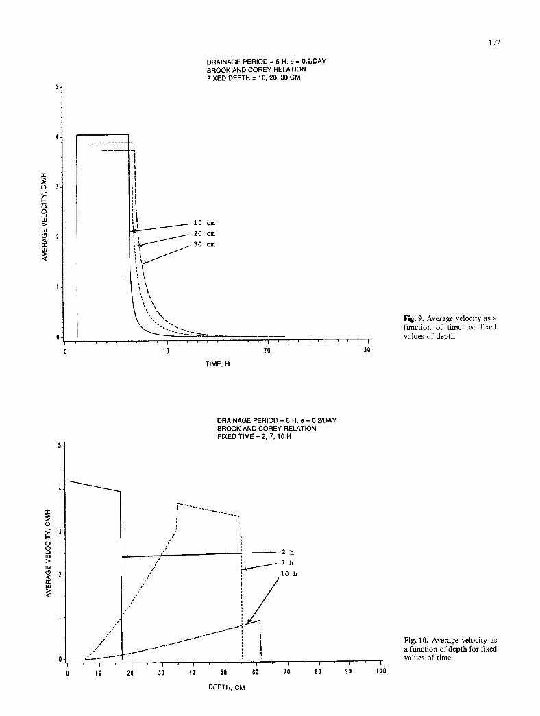
Fig. 9. Average velocity as a function of time for fixed values of depth

' 1 -

o >: I ' -

O _J i i i >

i l l (.9 < or" I i i > <

/

s " /

t ._

I

l0


i i i

, i i |

# i i , 2 h

�9 i L... .__-.- - T h

' ' 10 h

�9 i/ ,,

, i

' i

I I I I I

20 30 40 50 60

I I ' I

70 80 90

DEPTH, CM

!

I00

Fig. 10. Average velocity as a function of depth for fixed values of time

198

An example of application

A wetting event with moisture applied at the ground surface was considered, with K(O) given by Eq. (4). The soil was Glendale clay loam, investigated by Sisson et al. (1980), with the following properties: 0s=0.52, 0o = 0.246, K~ = 1 m/day, and a = 4.25. The moisture was applied at the rate of 2 cm/h for 6 hours. These values were used by Charbeneau (1984). The plant-root extraction e(t) was considered constant but values of e = 0.1, 0.2, 0.3, 0.4, and 0.5/day were considered. It should be emphasized that these values were used to illustrate the procedure presented in the paper. If n = 0.52, then e = 0.1/day would correspond to r(t)= 0.052/day. For one meter of soil column, this would translate into 5.2ram of plant-root extraction for a day. Likewise, e = 0.5/day would yield r(t) = 0.25/day or 25 mm/day. This rate is clearly high but the objective here was to intentionally show the modulation of soil moisture profile by the plant-root extraction.

The kinematic wave model was applied to compute O(z, t), q(z, t), and u(z, t). Then O(t), u(t) and q(t) were obtained at selected values of z. Likewise, O(z) and q(z) were computed at selected values of t. For a sample case of e = 0.2/day, computations are illustrated. Figure 5 shows O(t) at z = 10, 20, and 30 cm, and Fig. 6 shows O(z) at t = 2, 7 and 10 h. The moisture profile has realistic appearance. The moisture flux is plotted as a function of t in Fig. 7, and as a function of z in Fig. 8. The average velocity is plotted as a function of t in Fig. 9, and as function ofz in Fig. 10. Both q and u appear to be realistic in their variation. The effect of increasing e was to com- press domain/9 2 . In other words, after the moisture flux was ended at the ground surface, the moisture profile returned to its initial state more quickly where the moisture extraction rate was higher. For higher e, the characteristics in domain D1 were more curved.

Conclusions

The kinematic wave model for soil moisture movement has been formulated, and its solution domain involves three free boundaries. Analytical solutions are tractable for the case when the upstream boundary condition is independent of time. For a time-dependent boundary

condition, numerical solutions are the only resort. In this model, the advancing front of water or wetting front is necessarily an advancing shock wave. It is plausible to assume that the moisture content at the wetting front is 0o. Since the kinematic wave theory cannot account for this assumption, the diffusion wave model has to be em- ployed in that case.

Acknowledgements. This study was supported in part by Army Re- search Office under the project "A Continuum Model for Stream- flow Synthesis", Grant No. DAALO3-89-G-0116.

References

Brooks RH, Corey AT (1964) Hydraulic properties of porous media. Hydrology Paper 3, Colorado State University, Fort Collins, Colorado

Charbeneau RJ (1984) Kinematic models for soil moisture and solute transport. Water Resour Res 20:699 706

Charbeneau RJ, Weaver JW, Smith VA (1989) Kinematic modeling of multiphase solute transport in the vadose zone. EPA Report EPA/600/2-89/035, RS Kerr Environmental Research Labora- tory, U.S. Environmental Protection Agency, Ada, Oklahoma

Germann P (1985) Kinematic wave approach to infiltration and drainage into and from soil macropores. Trans ASAE 28: 745- 749

Germann P, Beven K (1985) Kinematic wave approximation to infiltration into soils with sorbing macropores. Water Resour Res 21 : 990-996.

Germann PF, Beven K (1986) A distribution function approach to waterflow in soil macropores based on kinematic wave theory. J Hydrol 83:173-183

Germann PF, Smith MS, Thomas GW (1987) Kinematic wave approximation to the transport of Escherichia coli in the vadose zone. Water Resour Res 23:1281-1287

Hsu R, Liu CL (1990) Use of parameter estimation in determining soil hydraulic properties from unsaturated flow. Water Resour Manag 4: 1-19

Irmay SE (1956) Extension of Darcy law to unsaturated flow through porous media. Proc Darcy Symposium, IASH-IUGG, Dijon, France

Sisson JB, Ferguson AH, van Genuchten MTh (1980) Simple method for predicting drainage from field plots. Soil Sci Soc Am J 44:1147-1152

Smith RE (1983) Approximate soil water movement by kinematic characteristics. Soil Sc Am J 47:3 8

Yamada T, Kobayashi M (1988) Kinematic wave characteristics and new equations of unsaturated infiltration. J Hydrol 102:257- 266

kinematic-wave model for soil-moisture movement with plant-root extraction

Documents