kim sharp entropy and the tao of counting a brief
TRANSCRIPT

123
Kim Sharp
Entropy and the Tao of CountingA Brief Introduction to Statistical Mechanics and the Second Law of Thermodynamics
SPRINGER BRIEFS IN PHYSICS

SpringerBriefs in Physics
Series Editors
Balasubramanian Ananthanarayan, Centre for High Energy Physics, IndianInstitute of Science, Bangalore, IndiaEgor Babaev, Physics Department, University of Massachusetts Amherst, Amherst,MA, USAMalcolm Bremer, H H Wills Physics Laboratory, University of Bristol, Bristol, UKXavier Calmet, Department of Physics and Astronomy, University of Sussex,Brighton, UKFrancesca Di Lodovico, Department of Physics, Queen Mary University ofLondon, London, UKPablo D. Esquinazi, Institute for Experimental Physics II, University of Leipzig,Leipzig, GermanyMaarten Hoogerland, University of Auckland, Auckland, New ZealandEric Le Ru, School of Chemical and Physical Sciences, Victoria Universityof Wellington, Kelburn, Wellington, New ZealandHans-Joachim Lewerenz, California Institute of Technology, Pasadena, CA, USADario Narducci, University of Milano-Bicocca, Milan, ItalyJames Overduin, Towson University, Towson, MD, USAVesselin Petkov, Montreal, QC, CanadaStefan Theisen, Max-Planck-Institut für Gravitationsphysik, Golm, GermanyCharles H.-T. Wang, Department of Physics, The University of Aberdeen,Aberdeen, UKJames D. Wells, Physics Department, University of Michigan, Ann Arbor, MI,USAAndrew Whitaker, Department of Physics and Astronomy, Queen’s UniversityBelfast, Belfast, UK

SpringerBriefs in Physics are a series of slim high-quality publications encompass-ing the entire spectrum of physics. Manuscripts for SpringerBriefs in Physics will beevaluated by Springer and by members of the Editorial Board. Proposals and othercommunication should be sent to your Publishing Editors at Springer.
Featuring compact volumes of 50 to 125 pages (approximately 20,000–45,000words), Briefs are shorter than a conventional book but longer than a journalarticle. Thus, Briefs serve as timely, concise tools for students, researchers, andprofessionals.
Typical texts for publication might include:
• A snapshot review of the current state of a hot or emerging field• A concise introduction to core concepts that students must understand in order to
make independent contributions• An extended research report giving more details and discussion than is possible
in a conventional journal article• A manual describing underlying principles and best practices for an experimental
technique• An essay exploring new ideas within physics, related philosophical issues, or
broader topics such as science and society
Briefs allow authors to present their ideas and readers to absorb them withminimal time investment.
Briefs will be published as part of Springer’s eBook collection, with millionsof users worldwide. In addition, they will be available, just like other books, forindividual print and electronic purchase.
Briefs are characterized by fast, global electronic dissemination, straightforwardpublishing agreements, easy-to-use manuscript preparation and formatting guide-lines, and expedited production schedules. We aim for publication 8–12 weeks afteracceptance.
More information about this series at http://www.springer.com/series/8902

Kim Sharp
Entropy and the Taoof CountingA Brief Introduction to Statistical Mechanicsand the Second Law of Thermodynamics

Kim SharpBiochemistry and BiophysicsUniversity of PennsylvaniaPhiladelphia, PA, USA
ISSN 2191-5423 ISSN 2191-5431 (electronic)SpringerBriefs in PhysicsISBN 978-3-030-35459-6 ISBN 978-3-030-35457-2 (eBook)https://doi.org/10.1007/978-3-030-35457-2
© The Author(s), under exclusive license to Springer Nature Switzerland AG 2019This work is subject to copyright. All rights are solely and exclusively licensed by the Publisher, whetherthe whole or part of the material is concerned, specifically the rights of translation, reprinting, reuseof illustrations, recitation, broadcasting, reproduction on microfilms or in any other physical way, andtransmission or information storage and retrieval, electronic adaptation, computer software, or by similaror dissimilar methodology now known or hereafter developed.The use of general descriptive names, registered names, trademarks, service marks, etc. in this publicationdoes not imply, even in the absence of a specific statement, that such names are exempt from the relevantprotective laws and regulations and therefore free for general use.The publisher, the authors, and the editors are safe to assume that the advice and information in this bookare believed to be true and accurate at the date of publication. Neither the publisher nor the authors orthe editors give a warranty, expressed or implied, with respect to the material contained herein or for anyerrors or omissions that may have been made. The publisher remains neutral with regard to jurisdictionalclaims in published maps and institutional affiliations.
This Springer imprint is published by the registered company Springer Nature Switzerland AG.The registered company address is: Gewerbestrasse 11, 6330 Cham, Switzerland

For Thi and Thuan

Preface
The second law of thermodynamics, which says that a certain quantity calledentropy always increases, is the law that scientists believe gives the direction totime’s arrow. It is the reason why so many everyday events happen only one way.Heat flows from hot to cold. Stirring milk into coffee always mixes it, never un-mixes it. Friction slows things down, never speeds them up. Even the evolutionof the universe and its ultimate fate depend on entropy. It is no surprise that thereare numerous books and articles on the subjects of entropy and the second law ofthermodynamics. So why write another book, even a short one, on the subject?
In 1854 Rudolf Clausius showed that there was a well-defined thermodynamicquantity for which, in 1865, he coined the name entropy. In his words “The energyof the universe remains constant. The entropy of the universe tends to a maximum.”Entropy could be measured and its behavior described, but what it was remained amystery. Twelve years later Ludwig Boltzmann provided the answer in atomistic,probabilistic terms and helped create the field of statistical mechanics.
Boltzmann’s explanation was the first, and arguably still the best, explanationof entropy. His classic paper, published in 1877, is probably never read anymoreyet something can still be learned by reading it. One of the things Boltzmannexplains very clearly is that there are two equally important contributions to entropy:one from the distribution of atoms in space and the other from the motion ofatoms (heat); in other words from the distribution of kinetic energy among theatoms.1 However, many introductory books and articles on entropy do not giveequal attention to each. The spatial contribution by its nature is just easier tovisualize and explain. Explanations of the kinetic energy contribution to entropyoften use fossilized concepts like Carnot cycles and efficiencies of heat engines. Itis also customary to teach thermodynamics before statistical mechanics, becausethe former is thought to be easier, and this follows their historical order of
1We now know of four sources of entropy in the universe. The third is radiation: photons haveentropy, a fact also discovered by Boltzmann. The fourth is black holes. These require a level ofphysics and mathematics beyond the scope of this book.
vii
viii Preface
development. Nevertheless, no purely thermodynamic description can explain whatentropy actually is. Nor can it explain the origin of the central concept, the famousBoltzmann distribution. This distribution is either introduced by fiat or derivedusing some fairly advanced mathematical techniques in a later statistical mechanicscourse which many students do not take. Either way, the result is an incompleteunderstanding of entropy.
My reason for writing this book is to go back to the beginning, as it were,and give a concise but accurate explanation of entropy and the second law ofthermodynamics. I take the contrary position that this can be done better by teachingstatistical mechanics before (or even without) thermodynamics and that this can bedone using just the basic concepts of mechanics: position, velocity, force, and kineticenergy. To do this I resurrect a very useful concept of Boltzmann’s, complexioncounting. A complexion is simply the list of positions and velocities of all the atoms.I use geometric arguments as much as possible, because these are more conducive tophysical understanding than calculus. I also give, for several of the most importantentropic effects, estimates of the huge numbers involved, again because this leads toa better physical understanding of entropy. The mathematics requires only a basicunderstanding of algebra, the exponential function and the logarithm function, at thelevel of an undergraduate majoring in the physical or biological sciences, or even ahigh school student with senior level physics.
Finally I want to thank my colleague Franz Matschinsky. His help, wisdom, andgood humor were essential in turning my rash decision to translate Boltzmann’sseminal 1877 paper on entropy into reality. As a result I was able to read it andfully appreciate the magnitude of Boltzmann’s achievements, which in turn led meto write this book.
Philadelphia, PA, USA Kim SharpAugust 2019

Contents
1 Learning to Count . . . . . . . . . . . . . . . . . . . . . . . . . . . . . . . . . . . . . . . . . . . . . . . . . . . . . . . . . . . . 1
2 What Is Entropy? . . . . . . . . . . . . . . . . . . . . . . . . . . . . . . . . . . . . . . . . . . . . . . . . . . . . . . . . . . . . . 19
3 Entropy and Free Energy . . . . . . . . . . . . . . . . . . . . . . . . . . . . . . . . . . . . . . . . . . . . . . . . . . . . 29
4 Entropic Forces. . . . . . . . . . . . . . . . . . . . . . . . . . . . . . . . . . . . . . . . . . . . . . . . . . . . . . . . . . . . . . . . 37
5 Summary . . . . . . . . . . . . . . . . . . . . . . . . . . . . . . . . . . . . . . . . . . . . . . . . . . . . . . . . . . . . . . . . . . . . . . . 49
Appendix . . . . . . . . . . . . . . . . . . . . . . . . . . . . . . . . . . . . . . . . . . . . . . . . . . . . . . . . . . . . . . . . . . . . . . . . . . . 55
References . . . . . . . . . . . . . . . . . . . . . . . . . . . . . . . . . . . . . . . . . . . . . . . . . . . . . . . . . . . . . . . . . . . . . . . . . . 59
Index . . . . . . . . . . . . . . . . . . . . . . . . . . . . . . . . . . . . . . . . . . . . . . . . . . . . . . . . . . . . . . . . . . . . . . . . . . . . . . . . 61
ix

Chapter 1Learning to Count
Abstract In 1877 Boltzmann explained the second law of thermodynamics in theseterms:
. . . the system will always rapidly approach a more probable state until it finally reachesthe most probable state, i.e. that of the heat equilibrium. . . . we will be able to identify thatquantity which is usually called entropy with the probability of the particular state.
Unpacking the meaning of this quote provides the key to understanding entropy.The term more probable simply means that some states or transformations betweenstates can happen in more ways than others. What we then observe in the real worldis that which can happen the most ways. This chapter first defines what is meant bythe term way, and then shows how to count these ways. In Chinese philosophy theterm Tao can be translated as ‘The Way’, so we may say that subject of this chapteris the Tao of counting.
Keywords Velocity · Kinetic energy · Temperature · Complexions · Friction ·Partition function
1.1 A Simple Analogy
As an introduction to this business of counting, consider rolling two dice. A possibleoutcome is a roll of 2 with dice number one, and a roll of 1 with dice number two,which will be abbreviated as (2, 1) (Fig. 1.1). Another outcome is a roll of (1, 2).This is a different outcome from the first roll because which dice has which roll isdifferent. Each possible outcome, defined as the specific values for each dice, willbe called a complexion. There are 6 × 6 = 36 possible complexions. Now we applya condition, for example that the spots on the dice must sum to a fixed value, and askhow many complexions satisfy that condition. If we require the sum to equal 7 forexample, there are six complexions that satisfy this condition: (1, 6), (2, 5), (3, 4),(4, 3), (5, 2), (6, 1). In contrast, a total of say 12 can be realized in just one way,
© The Author(s), under exclusive license to Springer Nature Switzerland AG 2019K. Sharp, Entropy and the Tao of Counting, SpringerBriefs in Physics,https://doi.org/10.1007/978-3-030-35457-2_1
1

2 1 Learning to Count
Fig. 1.1 Two dice, twocomplexions
(6, 6). The lesson from the dice analogy is that different conditions can be realizedby different numbers of complexions. We are very close to the meaning of entropywhen we recognize that in a large number of rolls of two dice we are likely to seea total of 7 more often than any other total simply because it is produced by morecomplexions than any other total. To understand thermodynamics, we need only toapply the same ideas to atoms.
1.2 Atoms Have Position and Velocity
Since we live in a three-dimensional universe we need three coordinates, x, y
and z, to describe the position of an atom, as shown in the left panel of Fig. 1.2.In addition, all atoms are in constant motion because they have thermal or heatenergy. More precisely, they have kinetic energy. Even atoms in a solid are movingrapidly back and forth. To describe the velocity of an object, we must not onlysay how fast it is moving—its speed in meters per second—but in what direction.For example, an airplane might be traveling west at 100 m/s, climbing at 10 m/s,and drifting north at 1 m/s because of a cross wind. To completely describe themotion of an atom we need to specify its speed in each of the x, y and z directions.These are the velocity components, u, γ and w illustrated in the right panel ofFig. 1.2.
The magnitude of the atom’s velocity, or its speed, can be calculated usingPythagoras’ theorem as
v =√
u2 + γ 2 + w2. (1.1)
v is the length of the velocity arrow in Fig. 1.2. In summary, at any moment in timean atom is described by three numbers for its position, and three numbers for itsvelocity, which will be abbreviated as a list of six numbers (x, y, z, u, γ,w).

1.3 The Kinetic Energy of an Atom 3
Fig. 1.2 Describing an atom by position and velocity
1.3 The Kinetic Energy of an Atom
An atom that is in motion has a kinetic energy proportional to its mass m, andproportional to the square of its speed v
Ek = 1
2mv2. (1.2)
Because the kinetic energy of an atom depends on the square of its speed the totalkinetic energy is the sum of the contributions from the x, y and z components ofvelocity:
Ek = 1
2mu2 + 1
2mγ 2 + 1
2mw2 (1.3)
This can be verified by substituting for v in Eq. 1.2 using Eq. 1.1. So we can speakof an atom as having three independent kinetic energy components.
If we have N atoms, the total kinetic energy is the sum of the atomic kineticenergies
EK = 1
2
N∑i
mi(u2i + γ 2
i + w2i ) (1.4)
where the subscript i labels the atom. The mean kinetic energy per atom isEK = EK/N . If N is large then the mean kinetic energy per atom and theabsolute temperature, T , are just the same thing but expressed in different units. Infact Maxwell and Boltzmann, when developing statistical thermodynamics, mostly

4 1 Learning to Count
used mean energy per atom not temperature.1 Because, in the development ofthermodynamics, the units of energy and the units of absolute temperature weredetermined independently the scale factor relating them had to be determinedempirically. This was done, for example, using the properties of an ideal gasand Boyle’s Law (see Appendix). It required knowing how many atoms are in agiven amount of material, i.e. knowing Avogadro’s constant. The relationship iskbT = 2
3 EK , where kb is called Boltzmann’s constant. If energy is measured inJoules and temperature is in degrees Kelvin then kb = 1.38 × 10⁻²³ J/K.
1.4 A Complexion of Atoms
If we have a collection of N atoms, at any moment in time we need 3N coordinates(xi, yi, zi) to specify the position of all the atoms in space and 3N velocitycomponents (ui, γi, wi) in the x, y and z directions, respectively, to specify themotion of all the atoms. The set of all 6N position-velocity coordinate values,
(x1, y1, z1, u1, γ1, w1 . . . xN , yN , zN , uN, γN,wN) (1.5)
defines what will be called a complexion. The term complexion is the Anglicizedform of the word Komplexion used by Boltzmann in his original work explainingentropy (Boltzmann 1877; Sharp and Matschinsky 2015). I resurrect this neutralterm to avoid baggage-laden terms such as microstate, disordered state, etc.often used in explaining entropy. Because the atoms are in motion the systemwill be continually moving from one complexion to another according to thelaws of dynamics. The set of 3N position coordinate values alone, (x1, . . . zN),will be referred to as a spatial complexion. Similarly, the set of 3N velocitycoordinate values alone, (u1, . . . wN), will be referred to as a velocity complexion,or equivalently, a kinetic energy complexion, since the kinetic energy componentsof the atoms are completely specified by their velocity components. Figure 1.3shows an example of four of the many possible complexions that three atomscould adopt.
1In their papers Maxwell and Boltzmann used the symbol T to refer to kinetic energy, nottemperature; a convention physicists still use today and a source of confusion.

1.5 Boltzmann’s Postulate 5
Fig. 1.3 Four possible complexions of three atoms. (a) and (b) have the same spatial complexion,but different velocity complexions, as do (c) and (d). (a) and (c) have the same velocity complexion,but different spatial complexions, as do (b) and (d). (a) and (d) have different spatial and velocitycomplexions, as do (b) and (c)
1.5 Boltzmann’s Postulate
Now that a complexion has been defined we introduce Boltzmann’s fundamentalpostulate.
Every complexion of N atoms having the same total energy E is equally likely
This is a postulate; it is not derived from any more fundamental principle. Itis, however, motivated by the principle of insufficient reason in the absence ofany definite knowledge to prefer one complexion over another (Bridgman 1972).Its ultimate justification must be how well the resulting theory explains observedthermodynamic behavior (Tolman 1938). Since statistical mechanics, within itsdomain of applicability, has proven to be an extremely reliable theory we have noreason to doubt Boltzmann’s fundamental postulate.
The next question, then, is how many complexions are there for a given numberof atoms with a given total energy? How can we count the ‘ways’ of arranging

6 1 Learning to Count
the atoms and their velocities? This task is described in the next section. WithBoltzmann’s postulate and the ability to count complexions we will then derive theSecond Law of Thermodynamics and the properties of entropy.
1.6 Counting Complexions: Part 1
The laws of dynamics describe how, given a set of atomic positions and velocitiesat some instant, these positions and velocities change with time. These laws do not,however, specify what positions and velocities are possible, only how they change.Without violating the laws of dynamics, any given spatial arrangement of atoms canin principle be combined with any given set of atomic velocities. In the languageof statistical mechanics positions and velocities are independent degrees of freedom(see, for example, Fig. 1.3). So we can split the task of complexion counting into twoparts. First, that of counting all possible velocity complexions with the same totalkinetic energy EK for any given spatial complexion. Second, accounting for thedifferent spatial complexions including, if necessary, any change in potential energywith atomic positions. In this section the machinery for counting velocity complex-ions is derived using a geometric argument and basic concepts of mechanics.
1.6.1 A Single Atom
Consider an atom i with velocity components (u, γ,w). It has kinetic energy
Ek,i = 1
2mi(u
2 + γ 2 + w2). (1.6)
The velocity of this atom can represented by a vector arrow which has a length,using Pythagoras’ theorem, of vi = √
2Ek,i/mi (Fig. 1.4). There are many othercombinations of x, y and z component velocities, (u′, γ ′, w′), that have the samekinetic energy provided that they satisfy the equation Ek,i = 1
2mi(u′2 + γ ′2 + w′2).
Each possibility corresponds to a velocity vector of the same length (magnitude)vi but representing a different velocity complexion. Every possible velocity com-plexion with the same kinetic energy can be represented by a vector starting at theorigin and ending somewhere on the surface of a sphere of radius R = √
2Ek,i/mi .Figure 1.4 shows two other velocity vectors of the same magnitude whose velocitiesdiffer by a small amount δv. It is clear from construction of this ‘velocity sphere’that the number of different velocity complexions Wv with fixed kinetic energy Ek,i
for atom i is proportional to the surface area of its velocity-sphere:
Wv ∝ R2 ∝ (√
Ek,i)2. (1.7)

1.6 Counting Complexions: Part 1 7
1.6.2 Many Atoms
Now consider N atoms with some velocity complexion (u1, γ1, . . . γN ,wN). Ini-tially we will consider the special case where all the atoms have the same mass m,and then generalize to atoms of different masses. The total kinetic energy is
EK = 1
2m
N∑i=1
(u2i + γ 2
i + w2i ). (1.8)
We can represent this velocity complexion as a vector in 3N-dimensional spacewith components (u1, γ1, . . . wN). By the 3N-dimensional version of Pythagoras’theorem this vector has length
√2EK/m. This is just the generalization of the
three-dimensional geometric picture of Fig. 1.4 to 3N dimensions. Then the numberof possible velocity complexions, Wv , with the same total kinetic energy isproportional to the surface area of a 3N -dimensional velocity-sphere of radiusR = √
2EK/m. The surface area of a 3N -dimensional sphere, A3N , is proportionalto R3N−1. In everything that follows we will be assuming that there is a largenumber of atoms, so we will now make the approximation 3N − 1 ≈ 3N to makethe equations tidier and the math easier to follow. So A3N ∝ R3N−1 ≈ R3N . SinceR ∝ E
1/2K the number of possible velocity complexions scales as
Wv ∝ E3N/2K (1.9)
with respect to the total kinetic energy. Now obviously the absolute numberof complexions depends on how finely we divide up the surface of the 3N -dimensional sphere; how small is the surface area element δA3N which represents
Fig. 1.4 Possible velocitiesof a single atom

8 1 Learning to Count
a single velocity complexion. However, all we will need are ratios of numbers ofcomplexions corresponding to some change in EK . So the size of the area elementδA3N will cancel out. To calculate changes in the number of complexions the onlything that matters is that this number scales as E
3N/2K .
1.6.3 The Effect of Heat on Velocity Complexions
One of Boltzmann’s most important discoveries was how to compute the change innumber of complexions when heat is added to the system (Boltzmann 1877). Hisoriginal derivation, which is followed by most textbooks of statistical mechanics, isquite involved mathematically and is thus hard to follow for the non-specialist. Sohere we pursue the geometric argument of Fig. 1.4. If a small amount of heat δQ isadded to a collection of N atoms, the kinetic energy increases from EK to EK +δQ.The radius of the 3N -dimensional sphere representing all possible velocity vectorsincreases by a factor of
R′
R=
(EK + δQ
EK
)1/2
=(
1 + δQ
NEK
)1/2
(1.10)
where EK is the mean kinetic energy per atom. The surface area of this sphereincreases by a factor of
(R′
R
)3N
=(
1 + δQ
NEK
)3N/2
. (1.11)
The number of complexions increases by the same factor as the surface area:
W ′v
Wv
=(
1 + δQ
NEK
)3N/2
, (1.12)
which can be re-written as
W ′v
Wv
= exp
(3N
2ln(1 + δQ/NEK)
)(1.13)
using the identity relationship between exponentials and logarithms: x = exp(lnx),and the fact that ln(xn) = nln(x). See the Appendix.
Since N is large, δQ << NEK and using the fact that ln(1 + x) ≈ x when x issmall (Appendix), we can make the approximation:
ln(1 + δQ/NEK) ≈ δQ/NEK. (1.14)

1.6 Counting Complexions: Part 1 9
Substituting this approximation into the exponent gives Boltzmann’s equation
W ′v
Wv
= exp
(3
2
δQ
EK
)= exp
(δQ
kbT
)(1.15)
where the second equality uses the relationship of Sect. 1.3 between temperatureand mean kinetic energy, namely kbT = 2
3 EK .
1.6.4 Accounting for Atoms with Different Masses
We now generalize the argument leading to Eq. 1.15 for atoms with different masses.Equation 1.8 for the total kinetic energy is now replaced by
EK = 1
2
N∑i=1
mi(u2i + γ 2
i + w2i ). (1.16)
Equation 1.16 can be rewritten as
1 =N∑
i=1
(u2
i
a2i
+ γ 2i
a2i
+ w2i
a2i
) (1.17)
where ai = √2EK/mi . This is the equation for a 3N-dimensional ellipsoid with
semi-axes of length ai . For the same kinetic energy a lighter atom has a greatervelocity than a heavy atom. So the 3N-dimensional velocity-sphere becomes elon-gated along the axial directions of lighter atoms, and shortened along the directionsfor heavier atoms, becoming an ellipsoid. All possible velocity complexions forfixed EK are represented by a 3N -dimensional vector from the center of thisellipsoid ending somewhere on its surface. The argument about how the numberof complexions depends on EK is the same as for the equal mass/sphere case: Wv
is given by how many different 3N-dimensional velocity vectors there are, whichis proportional to the surface area of the 3N-ellipsoid. This ellipsoid is of fixedshape determined by the various masses of the atoms. Thus its surface area scales asthe (3N − 1)th ≈ (3N)th power of the linear dimension of the ellipsoid. The linear
dimension scales as√
EK , so the area scales as the 3N2
thpower of EK as before. The
addition of a small amount of heat provides the same factor of (1 + δQ/NEK)3N/2
for the number of complexions. For δQ << NEK this leads again to Boltzmann’sequation 1.15.

10 1 Learning to Count
1.6.5 The Meaning of Boltzmann’s Equation
Equation 1.15 says that if a small amount of heat (kinetic energy) δQ is addedto N atoms that have average kinetic energy EK , then the number of velocitycomplexions increases by a factor of W ′
v/Wv given by Eq. 1.15 where Wv andW ′
v are the number of velocity complexions before and after the heat addition. Theincrease in number of velocity complexions comes from the increase in the numberof ways to distribute the kinetic energy among the N atoms. Conversely, if weremove heat (δQ is negative) the number of complexions decreases. The exponentialform of Eq. 1.15 is a reflection of the combinatoric nature of complexion counting.For example, if we add an amount of heat equal to the average kinetic energy of oneatom, EK , the increase in velocity complexions is a factor of e3/2 = 4.48. If twiceas much heat is added, then the number of complexions increases by the square ofthis factor, about 20-fold.
Another feature of Boltzmann’s equation is that the effect of a given incrementof heat depends on how much heat is already there; how large δQ is compared to theaverage kinetic energy of the atoms. In terms of the geometric picture of Fig. 1.4,the increment in radius of the velocity sphere due to a fixed amount of heat δQ
increases the surface area of the 3N-sphere by a larger factor when the radius of thesphere (which is proportional to
√EK ) is smaller. The proportionally larger effect
of heat added at a lower temperature is graphically illustrated in Fig. 1.5 using thevelocity sphere of a single atom. Here 2 units of kinetic energy are added to an atomstarting with 4 units of kinetic energy (low T) or starting with 8 units of energy (highT). It is apparent from the figure, which is drawn to scale, that the area of the low Tsphere (on the left) is increased by a larger factor than the high T sphere.
Most of what follows will make use of Boltzmann’s equation 1.15. Before wemove on to complete the counting of complexions, the next section gives twoapplications of this equation to demonstrate its explanatory power.
Fig. 1.5 Effect of addingheat is greater at lowertemperature

1.7 Why Heat Flows from Hot to Cold 11
1.7 Why Heat Flows from Hot to Cold
If we examine Boltzmann’s equation 1.15 we see that in the exponent the amountof heat δQ is divided by the mean kinetic energy per atom, EK . A given amountof heat will cause a greater increase in the number of velocity complexions (waysto distribute the kinetic energy) when it is added to a collection of atoms with asmaller amount of kinetic energy, i.e. with a lower temperature (see Fig. 1.5). Soif a small amount of heat leaves a body A at temperature TA and enters a body B
at a lower temperature TB it is clear that the number of velocity complexions for A
decreases by a smaller factor than that by which the number of velocity complexionsfor B increases, because TB < TA. The total number of velocity complexionsis the product of the complexion numbers of A and B, so the total changes by afactor
W ′
W= W ′
AW ′B
WAWB
= exp
(δQ
kb
(1
TB
− 1
TA
)). (1.18)
This factor is greater than one because 1/TB > 1/TA and the exponent ispositive. If heat flowed in the reverse direction, from cold to hot, the number ofcomplexions would decrease, which by Boltzmann’s fundamental postulate meansit is less likely to be observed. So heat will flow from A to B until the numberof complexions stops increasing, i.e. reaches a maximum. This happens whenTB = TA, which is thermal equilibrium. Put another way, when TB = TA,the exponent in Eq. 1.18 is zero, so the ratio W ′/W is one. The transfer of asmall amount of heat in either direction does not change the number of velocitycomplexions.
The real import of counting complexions comes when representative numbers arecalculated. Take two 0.1 kg blocks of copper. One is at a temperature of 300 K. Theother is one millionth of a degree hotter at 300.000001 K. From the heat capacityof copper, 385 J/kg/K, we can calculate how much more heat the hotter block has:38.5µJ. To equalize the temperature, half of this extra heat must flow into the colderblock. Evaluating Eq. 1.18 with δQ = 19.25µJ and kb = 1.38 × 10⁻²³ J/K theexponent has a value of about 7.8 × 10⁶, giving
W ′
W= e7.8×106 ≈ 103,400,000. (1.19)
The number of kinetic energy complexions increases by a factor of 1 followed bymore than three million zeros.2 The equal temperature situation has overwhelminglymore complexions. Clearly the possibility of anything more than a really micro-scopic flow of heat in the reverse direction, from cold to hot, is close to zero.
2Using ex = 10(x/ ln10), ln10 = 2.303. See Appendix.

12 1 Learning to Count
[Technical note: Equation 1.15 was derived assuming that the change in temper-ature upon addition of the heat was negligible, while of course in the above thermalequilibration example the temperature of A does change, from TA to TA − ΔT/2,while that of B changes from TB to TB + ΔT/2, where ΔT = TA − TB . So thecalculation was done assuming constant temperatures for A and B equal to their“average values” during the equilibration, namely TA − ΔT/4 and TB + ΔT/4. Forthis example the error compared to the exact result (obtained by integration over acontinuous temperature change) is tiny.]
1.8 Why Friction Slows Things Down
A rubber ball is released from a certain height above a smooth hard surface. Itaccelerates downwards, Fig. 1.6, hits the surface, bounces up a few times, eachtime to a lesser height until finally it comes to rest on the surface. Since energy isconserved why does this happen, why does the ball not bounce back to the originalheight and keep on bouncing for ever? Or why cannot the ball, after remaining at restfor a while, spontaneously move upwards to its initial height? Initially the ball has acertain potential energy mgh where m is the mass of the ball, h is the release heightabove the surface, and g is the acceleration due to Earth’s gravity. This potentialenergy is converted into the kinetic energy of the ball’s motion, EK = 1
2mv2 =mgh, where v is the speed of the ball when it reaches the surface. How many waysare there to distribute this kinetic energy among the atoms of the ball? In effect, justone, where all atoms have identical velocity components (u, γ,w) = (0, 0,−v)
equal to the center of mass motion. When the ball comes to rest this kineticenergy has been converted to exactly the same amount of heat: kinetic energy nowdistributed at random among the atoms of the ball, the surface, the air.
Boltzmann’s equation 1.15 tells us how the number of velocity complexions hasincreased. For example take a 0.1 kg ball released from a height of 0.1 m, at roomtemperature, 300 K. The gravitational constant is g = 10 m/s2, so δQ = 0.1 J. The
Fig. 1.6 Friction slowsobjects down

1.9 Why Is the Number of Complexions So Large? 13
exponent in Eq. 1.15 is 2.42 × 10¹⁹. The number of complexions increases by afactor
W ′
W= e2.42×1019 ≈ 101019
. (1.20)
In other words, the number of complexions increases by a factor of 1 followed byten quintillion (1019) zeros. This is a mind-bogglingly large number. No wonderthe effect of friction is irreversible and the kinetic energy components in thesurroundings could never spontaneously ‘line up’ to push the ball back up in theair once it has come to rest.
1.9 Why Is the Number of Complexions So Large?
In the previous two sections we encountered some extremely large numbers. It ishelpful to understand what is the origin of these large numbers, and just how largethey are. This is key to understanding why the Second Law of Thermodynamics,even though it is statistical, is called a law.
The large numbers are a consequence of one physical factor and one mathemat-ical factor. On the physical side, atoms are extremely small, which is reflected inthe fact that Avogradro’s number is large: 6.02 × 10²³ molecules per mole. Thismeans that even a nanoscale amount of matter contains a lot of atoms. One billionthof a gram of diamond, for example, still contains about 5 × 10¹³ atoms of carbon,although this number is unlikely to impress one’s fiancée! The mathematical sideinvolves permutations, which describe the number of ways of arranging things (hereatoms or atomic velocities). The number of permutations increases very rapidlywith the number of things. Roughly speaking permutations scale as nn, where n
is the number of things. We say that a number like en or 10n, where n occurs in theexponent, increases literally exponentially with n. But with permutations n occurs asthe base and the exponent, so permutations increase supra-exponentially. Put thesetwo factors together and numbers like 103.4×10⁶
and 101019are the result.
It is not accurate to call these numbers astronomical, because astronomicalnumbers like the number of atoms in the universe (on the order of 1079), areby comparison small. Even a googol, the archetypal large number, has only onehundred zeros after the 1, and so it is also a piker in comparison. A better yardstickis the proverbial monkey plinking away randomly on a typewriter and producing theexact text of Hamlet. Say Hamlet contains about 27,000 characters, including spacesand punctuation. We’ll be strict and want correct capitalization and punctuation,so there are 26 upper and lower case characters to choose from, plus the spaceand say seven punctuation symbols, for a round total of 60 possible symbols ateach of 27,000 positions. The odds are 1:6027,000 ≈ 1:1048,000 against the monkeyproducing Hamlet. But this involves a number which is not even close to the smallerof the two complexion numbers occurring in the previous two examples.

14 1 Learning to Count
1.10 Counting Complexions: Part 2
In Sect. 1.6 we derived the number of velocity complexions as a function ofthe total kinetic energy for any given spatial complexion. We now add in thespatial complexion contribution to provide a complete prescription for complexioncounting.
1.10.1 Combining Spatial and Velocity Complexions
We again have a collection of N atoms with total kinetic energy EK . First assumethat there are no forces acting on the atoms, either from other atoms or from externalfactors. This means that there is no variation in potential energy with the positionsof the atoms. In this case if there are Ws spatial complexions each can be combinedwith all Wv possible velocity complexions having the same total kinetic energy EK .This gives a total of
W = Ws × Wv (1.21)
complexions. An example in miniature is shown in Fig. 1.3. Here there are twodifferent spatial complexions which are combined with two different velocitycomplexions to give a total of four complexions. If we apply Boltzmann’s postulateto Eq. 1.21, what it tells us is that in the absence of forces each spatial complexion isequally likely, since each can be combined with exactly the same number of velocitycomplexions.
Now assume that there are forces acting. Equation 1.21 no longer applies. Whenan atom moves its potential energy is changed according to the relationship
δU = −f δx (1.22)
where δx is the displacement along the direction of a force of magnitude f . If theatom moves in the direction of the force its potential energy decreases, in otherwords it moves downhill in potential energy. This energy is converted into kineticenergy as the atom is accelerated according to Newton’s Third Law: f = ma. Thereverse is true if the atom moves against the force. The atom slows down and loseskinetic energy as it moves uphill in potential energy. Since energy is conserved andthere are only two types of energy, kinetic and potential, we have
δQ = −δU.
It is immaterial whether the forces are external or come from interactions betweenthe atoms: When there is a change in potential energy heat is created or annihilated,depending on the sign of the change. Because of this heat change, what Boltzmann’skey discovery, Eq. 1.15, tells us is that the corresponding spatial complexions arenow no longer equally likely, because each has a different number of possible

1.10 Counting Complexions: Part 2 15
Fig. 1.7 At higher potentialenergy atoms have fewervelocity complexions
velocity complexions available to it. With constant total energy, spatial complexionsof higher potential energy have lower kinetic energy. Therefore they have lesskinetic energy complexions and so they are less likely, and vice versa. This isillustrated qualitatively in Fig. 1.7 for the velocity sphere of a single atom at twopositions of different potential energy.
To quantify the effect of potential energy on complexions in the general case,first compare two spatial complexions of N atoms, labelled A and B which havedifferent potential energies: UA and UB . When the atoms move from complexion A
to complexion B an amount of heat −(UB − UA) is created if we move downhillin potential energy (UB < UA) or is annihilated if we move uphill in potentialenergy (UB > UA). Using Eq. 1.15 the ratio of the corresponding number of velocitycomplexions is
Wv(B)
Wv(A)= exp
(− (UB − UA)
kbT
)(1.23)
Thus the two spatial complexions A and B actually correspond to W(A) = 1 ×Wv(A) and W(B) = 1 × Wv(B) total complexions, respectively. By Boltzmann’sfundamental postulate, the relative probability of being in the spatial complexionB vs. the spatial complexion A is given by the ratio of their total numbers ofcomplexions
pB
pA
= exp
(− (UB − UA)
kbT
)(1.24)
Put another way, the presence of potential energy has introduced a coupling betweenthe spatial and velocity complexions. From Eq. 1.24 it follows that we can write theabsolute probability of any spatial complexion i as
pi = exp(−Ui/kbT )∑Ws
i=1 exp(−Ui/kbT )(1.25)

16 1 Learning to Count
since any pair of probabilities pi and pj given by Eq. 1.25 satisfy Eq. 1.24, and theprobabilities sum to one. The probability distribution pi is called the Boltzmanndistribution. The term e−Ui/kbT in the numerator is called the Boltzmann factor.The sum of these factors in the denominator is taken over all possible spatialcomplexions Ws . This sum functions as a probability normalizing factor and in spiteof its mundane origin it plays an important role in entropy and statistical mechanics.Because of this it is given a name, the partition function, often denoted by thesymbol Z from the German Zustandssumme (literally sum of states):
Z =Ws∑i=1
exp(−Ui/kbT ) (1.26)
Using Eq. 1.25 we can now calculate the average value of any property X using
X =Ws∑i=1
piXi = 1
Z
Ws∑i=1
Xi exp(−Ui/kbT ) (1.27)
where Xi is the value of the property in the ith spatial complexion. For example themean potential energy is given by
U =Ws∑i=1
piUi = 1
Z
Ws∑i=1
Ui exp(−Ui/kbT ) (1.28)
1.10.2 The Total Number of Complexions
To obtain the total number of complexions W available to a fixed number of atomsN with fixed total energy E we need to sum the number of velocity complexionsavailable to each spatial complexion:
W =Ws∑i=1
Wv(i) (1.29)
where in general Wv(i) will vary from spatial complexion to spatial complexiondepending on that complexion’s potential energy. We will pick an arbitrary spatialcomplexion o, with potential energy Uo as a reference and use Eq. 1.23 to write thenumber of velocity complexions possible with spatial complexion i in terms of thenumber of velocity complexions of the reference state:
Wv(i) = Wv(o) exp
(−(Ui − Uo)
kbT
)(1.30)

1.10 Counting Complexions: Part 2 17
The total number of complexions is then given by
W = Wv(o) exp(Uo/kbT )
Ws∑i=1
exp(−Ui/kbT ) = C′Z (1.31)
The factor coming from the arbitrary complexion o used as a reference state iscommon to all the spatial complexions. It is brought outside the sum as a constant,C′. The sum itself is just the partition function Z of Eq. 1.26.
1.10.3 Constant Temperature Conditions
Equation 1.31 gives the total number of complexions for a fixed number of atomswith a constant total energy E. This assumes that the collection of N atoms we areinterested in is completely isolated from its environment: No heat can enter or leave,which is known as adiabatic conditions. The more common situation is a system inthermal equilibrium with its surroundings, i.e. under constant temperature condi-tions. How does this affect the counting of complexions? We can apply the resultsfrom the heat flow example, Sect. 1.7 to find out. Consider our collection of N atomsat equilibrium with its surroundings at a temperature T . At a certain moment thiscollection has total energy E. The total number of complexions is given by Eq. 1.31.Since it is in thermal equilibrium with its surroundings, say a small fluctuation (dueto collisions with its surroundings, or thermal radiation emitted or received) causes asmall amount of heat δQ to pass from the surrounding environment to the system orvice versa. Although Eq. 1.15 says that the number of complexions for the system ofN atoms changes, application of Eq. 1.18 with TA = TB = T shows that the numberof complexions of the surroundings changes by an equal and opposite amount, sothat the total number of complexions (of system plus environment) is unaffected bythe heat flow allowed by constant T conditions: Complexion counting is the sameas though we kept the system at constant energy E.
SummaryComplexion counting has produced the following results
• Equation 1.9: The number of kinetic energy complexions is proportionalto the total kinetic energy raised to the 3N/2th power,
Wv ∝ E3N/2K
where N is the number of atoms.
(continued)

18 1 Learning to Count
• Equation 1.15: If a small amount of heat δQ is added, the number of kineticenergy complexions is increased by the factor
W ′v
Wv
= exp
(δQ
kbT
)
• Equation 1.21: When there are no forces acting the total number of com-plexions is the product of the number of spatial and velocity complexions
W = Ws × Wv
and all spatial complexions are equally likely.• Equation 1.25: When there are forces acting there are potential energy
differences, and the probability of a spatial complexion i depends on thepotential energy of that complexion and the temperature as
pi = exp(−Ui/kbT )∑Ws
i=1 exp(−Ui/kbT )
• Equation 1.31: The total number of complexions is proportional to thepartition function
W ∝Ws∑i=1
exp(−Ui/kbT )
where the sum is over all possible spatial complexions, and the terms inthe sum are the Boltzmann factors.
With the ability to count complexions and determine their probabilities wecan now explain what we see at equilibrium, by determining what state hasthe most complexions. To paraphrase Feynman (1972) much of statisticalmechanics is either leading up to the summit of Eqs. 1.25 and 1.27 or comingdown from them. In this chapter on complexion counting we proceededentirely without the concept of entropy. Historically, however, entropy wascharacterized as a thermodynamic quantity before its molecular, statisticalorigins were known. So in the next chapter we connect the concepts ofcomplexion counting and entropy.

Chapter 2What Is Entropy?
Abstract In this chapter Clausius’ 1865 macroscopic, thermodynamic definitionof entropy is united with Boltzmann’s 1877 atomistic, probabilistic definition ofentropy.
Keywords Equilibrium · Entropy · Ideal gas · Barometric equation ·Maxwell-Boltzmann distribution
2.1 The Statistical, Atomistic Definition of Entropy
In principle, Boltzmann’s postulate combined with the methods just describedfor counting complexions are enough to understand equilibrium thermodynamics.Historically, however, Clausius had already defined a quantity he called entropy, andhe showed by thermodynamic arguments that the entropy change in any substanceproduced by a small amount of added heat is given by
δS = δQ
T(2.1)
where δQ is small enough that it causes a negligible change in temperature. But thisratio of added heat to temperature is just what appears in the exponent of Eq. 1.15.If we substitute Eq. 2.1 in and take the logarithm of both sides we get:
δS = kbln
(W ′
v
Wv
)(2.2)
The change in entropy is due to the change in the number of complexions; thechange in the number of ways to distribute the kinetic energy among the atoms. Theequivalence in Eq. 2.2 led Boltzmann to a more general definition of the entropy ofa state in terms of the total number of complexions for that state
S = kblnW + C (2.3)
© The Author(s), under exclusive license to Springer Nature Switzerland AG 2019K. Sharp, Entropy and the Tao of Counting, SpringerBriefs in Physics,https://doi.org/10.1007/978-3-030-35457-2_2
19

20 2 What Is Entropy?
where W includes both spatial and velocity complexions. The more generalexpression for a change in entropy is then
ΔS = kbln
(W ′
W
)(2.4)
The use here of the notation ΔS instead of δS indicates that Boltzmann’s expressionis valid for any size change of entropy.
C in Eq. 2.3 is an undetermined constant which is unimportant since we arealways interested in changes in entropy, so it is convenient to set C = 0. Thenthe logarithmic relationship between entropy and complexions means that entropiesof independent systems are additive because the total number of complexions is theproduct of each system’s complexion number.
In Eqs. 2.2–2.4 the units of entropy are energy per degree of temperature, e.g.J/mol/K. So the numerical value depends on the units being used. However, S/kb
is dimensionless. Only dimensionless quantities have physical meaning, but morecommonly units of energy per degree Kelvin are used. The crucial point is thatentropy is simply a logarithmic measure of the number of complexions. As wehave seen it is often insightful to express results directly in terms of numbersof complexions rather than in entropy units: Although the molecular definition ofentropy is probabilistic, appreciation of the numbers involved more clearly conveysthe almost deterministic nature of entropic effects at the observable level.
2.2 Entropy Maximization Explains Equilibrium Behavior
Thermodynamics deals with quantities like pressure, the distribution of gasesor liquids and equilibrium constants of chemical reactions. These are averagequantities involving large numbers of atoms, what are called macroscopic quantities.In this context Boltzmann’s postulate about equi-probable complexions simplymeans:
The macroscopic state that we see at equilibrium is the state that can happenin the most ways; that corresponds to the most complexions.
This principle is illustrated in miniature by the dice analogy: If you roll two dice,the ‘macroscopic’ total of 7 is the most likely because 6 of the 36 complexions,(1,6), (2,5), (3,4), (4,3), (5,2) and (6,1) produce this total, more complexions thanfor any other total. We will observe a total of 7 on average one sixth of the time.
Equation 2.3 formalizes Boltzmann’s identification of the most probable state,the state that can happen the most ways, with the state of maximum entropy. Whatmust be appreciated is that when you deal with the typical number of atoms involved

2.2 Entropy Maximization Explains Equilibrium Behavior 21
Fig. 2.1 Equilibrium distribution of atoms
in a real world situation, the state with the most complexions dominates to an almostunbelievable degree.
Consider 100 million gas molecules distributed between two equal volumes,labeled left and right in Fig. 2.1. Each molecule could be in either the left handvolume or the right hand volume. So at this macroscopic level of description thereis a total of 2N different spatial complexions. A particular macroscopic distributionwould be L molecules in the left-hand volume, and R = N − L molecules in theright-hand volume. The number of spatial complexions in this macroscopic state isthe different number of ways of splitting N molecules into two groups with L in onegroup, R in the other. This is given by the binomial distribution
W(L) = N !L!R! (2.5)
Here N ! = N × (N − 1) × (N − 2) . . . × 1, etc. are factorial functions. A graph ofW(L) is shown in the central panel of Fig. 2.1. The abscissa gives the distribution interms of the percentage of molecules in the left hand volume. So 50% correspondsto an equal or 50:50 distribution. Note that the distribution is so narrowly peakedaround L = R that the abscissa scale is greatly expanded, with a range of just 49–51%. The real story comes by putting the numbers into the binomial formula. If wemove away from the equi-distribution peak at 50:50 by just a small amount, 0.25%,the number of complexions falls by a staggering factor of 1/10543. Furthermore, ifwe calculate what fraction of all 2N complexions is contained in the narrow rangeof distributions from 49.98:50.02 to 50.02:49.98 spanning this peak, we find that itcontains more than 99.993% of all complexions.
In other words almost every complexion is indistinguishable from the most likely,50:50, state. The most likely state, plus all those states that are macroscopicallyindistinguishable from it, account for all but a very very very tiny fraction ofall complexions. Since all complexions are equally likely, we will almost neverstray from one of the typical equilibrium-like complexions. The percentages in this

22 2 What Is Entropy?
example are for 100 million molecules, which is a rather small amount of matter,about 5 million billionths of a gram of oxygen gas. For truly macroscopic amounts ofmatter the complexions will cluster even more closely around the maximum entropy50:50 state.
It is also important to understand what Boltzmann’s postulate is not saying. It isnot saying that the macroscopic behavior is a result of the atoms exploring all thecomplexions (the so-called ergodic hypothesis), or even most of the complexions.Even for this small system of 100 million atoms and at this coarse level ofdescription the total number of complexions is about 1 followed by 30 millionzeros. The system can only explore a tiny fraction of the possible complexions in thetime we observe it. Therefore it will almost never encounter the vanishing minorityof complexions that are detectably unlike the most probable or maximum entropystates.
2.3 The Maximum Entropy State for Gas, Mixturesand Solutes Is Uniform Density
The partition of the volume in Fig. 2.1 into left and right regions is arbitrary. Anotherequi-volume partition is illustrated by the checkerboard pattern in the lower leftof the figure. The same argument about distributions applies to any equi-volumedivision: almost all complexions will correspond to an equal distribution. Fromthis we conclude that in the absence of external forces the maximum entropydistribution, the one that can happen the most ways, the one that represents all thosethat will be observed at equilibrium, is a uniform distribution of gas in the availablevolume.
Now let the gas initially be confined to one volume. Then a valve is opened to asecond, equal volume, as in the right panel of the figure. As the gas molecules movefrom one complexion to another because of their thermal motion, over time theyare overwhelmingly likely to end up in the equilibrium-like complexions, the oneswith the gas equally distributed between the volumes, simply because almost everycomplexion is like this. So the gas expands to uniformly occupy all the volume.This is not because the second volume has a vacuum—in fact the expansion willoccur even if the second volume is filled with a different gas. The mixing of thetwo gases is just a by-product of each gas moving independently to states for whichthere are the most complexions. A similar argument applies to mixing of liquids: Adrop of ink mixing with water, or milk stirred into coffee. The molecules of ink ormilk are simply moving to complexions belonging to the most likely distribution—auniform distribution in their available volume. Similarly with any solute dissolvedin a solvent. The counting of solute spatial complexions is analogous to that of a gasin the same volume as the solution. If there are no strong interactions between thesolutes, and the solute concentration is not too high, then the most likely distributionis a uniform density.

2.4 The Entropy of an Ideal Gas 23
To put in some numbers, consider 10 cm3 of gas at a pressure of 1 atm and atemperature of 273 K. There are about N = 2.4 × 10²⁰ molecules of gas (using amolar volume of 24.6 L, and Avogadro’s number, 6.02×10²³). If this gas is allowedto expand into twice the volume, the number of complexions goes up by a factor of2N ≈ 101020
, which is 1 followed by about 100 quintillion zeros. That gas is notgoing to spontaneously go back into the smaller volume any time soon.
2.4 The Entropy of an Ideal Gas
An ideal gas is one in which the molecules have no volume, and make nointeractions. The molecules are basically modelled as points, whose only propertiesare mass, position and velocity. An ideal gas is also a good model for gaseslike nitrogen, oxygen and argon at normal temperatures and pressures. For thesereasons it is often used to illustrate thermodynamic principles. Since there areno forces, the total number of complexions is given by Eq. 1.21. The number ofvelocity complexions according to Eq. 1.9 is proportional to E
3N/2K and so it is also
proportional to T 3N/2, since temperature is proportional to the total kinetic energyfor a fixed number of atoms. For the spatial complexions, we imagine the volumeV occupied by the gas to be divided up into a large number of small cubic regionsof equal volume b. There are V/b ways of placing a single molecule into one ofthe small boxes. In an ideal gas the molecules are all independent of each other sothere are (V/b)2 ways of placing two molecules into the boxes, and so on. Thusthe total number of spatial complexions is proportional to V N . Clearly the absolutenumber of spatial complexions depends on how finely we divide space, but for anyprocess of interest involving a volume change, the entropy change will depend onthe ratio of the numbers of complexions, and b will cancel out. Putting the spatialand velocity complexion results together, the total number of complexions for anideal gas is
W ∝ V NT 3N/2 (2.6)
The ideal gas entropy is then
Sid = NkblnV + 3
2NkblnT + C (2.7)
Note the spatial and velocity contributions to the entropy are additive, which followsfrom what was said earlier, that in the absences of forces the spatial and velocitycomplexions can be realized independently of the other, so the total number ofcomplexions is given by their product (Eq. 1.21). Again, C is a constant of nointerest since it does not depend on T or V and so it will cancel out for any changein these two thermodynamic quantities.

24 2 What Is Entropy?
2.5 The Spatial Distribution of a Gas Under Gravity:The Barometric Equation
One of Boltzmann’s very first applications of the distribution that now bears hisname was to the distribution of a gas in a gravitational field (Boltzmann 1877).Taking an altitude of zero (mean sea level) as a reference, the potential energy of agas molecule of mass m at a height h above sea level is mgh. Then Eq. 1.24 givesthe probability of that gas molecule being at height h as
p(h) ∝ exp
(−mgh
kbT
). (2.8)
Consequently the density (and pressure) of gas has the distribution
ρ(h) = ρ(0) exp
(−mgh
kbT
)(2.9)
where ρ(0) is the density at sea level. Using an approximate molecular weight of30 g/mole for atmospheric gas, the mass per molecule is 5×10⁻²⁶ kg, g = 10 N/kg.With T = 300 K and kb = 1.38 × 10⁻²³ J/K, the factor kbT /mg has the value8280 m. In other words, the equation gives an atmospheric density half that ofsea level at about 5700 m, or 70% of the way up Mt. Everest. Here we are notcorrecting for the decrease in temperature with altitude. Equation 2.9 is known as thebarometric equation. It gives the maximum entropy arrangement of gas moleculesin the atmosphere at constant temperature. This demonstrates that the principle ofmaximum entropy can operate on a very large scale. Note that on the laboratoryscale, these variations in density with height are tiny, so the uniform distribution ofSect. 2.3 is still the maximum entropy distribution.
2.6 The Distribution of Velocities at Equilibrium
Sections 2.3 and 2.5 give the maximum entropy spatial distributions of a gas underdifferent conditions. We now consider the maximum entropy distribution of kineticenergy in a gas. As illustrated in Fig. 1.4, for a fixed total kinetic energy EK all thepossible velocity complexions can be represented by a 3N -dimensional vector oflength R = √
2EK/m, 3N being the number of velocity terms. Since these velocityvectors are of constant length R they trace out the (3N − 1)-dimensional surface ofa 3N -sphere, the number of degrees of freedom being reduced by one because ofthe constant energy constraint. We can use the velocity-sphere concept to describethe equilibrium distribution of kinetic energy/velocity components in more detail.
First, we know from Sect. 1.7 on heat flow that in a region containing a largenumber of atoms the temperature should be uniform, i.e. on average the kinetic

2.6 The Distribution of Velocities at Equilibrium 25
energy is uniformly distributed. However this does not mean that at the atomiclevel at any particular moment all the atoms have exactly the same kinetic energy,distributed equally among the x, y and z components. In fact this completelyuniform distribution is very unlikely: It corresponds to a complexion where |u1| =|γ1| = |w1| = |u2| = . . . |wN |. Geometrically, this corresponds to a specialdirection in 3N-dimensional space for the velocity vector, namely aligned exactlyon one of the 3N diagonals. But there many more non-diagonal directions in the3N -dimensional sphere to which the velocity vector could point. Thus there will bea range of velocities among the atoms. The form of this velocity distribution can beobtained from the velocity-sphere, as follows.
Consider any component of the velocity of any atom, say the x component ofthe ith atom. If the distribution of velocity vectors is uniform over the (3N − 1)-dimensional surface of the velocity sphere, as per Boltzmann’s postulate, then whatis the probability distribution of this velocity component? If this velocity componenthas a particular value ui , where −R � ui � +R, and R = √
2EK/m is the radius ofthe velocity sphere, then this constrains all possible 3N-dimensional velocity vectorsto trace a (3N − 2)-dimensional ‘circle’ C of radius
Rc =√
R2 − u2i = R
(1 −
12mu2
i
EK
)1/2
(2.10)
on the (3N − 1)-surface, see Fig. 2.2. In Eq. 2.10 12mu2
i is the x component of thekinetic energy of atom i.
Technically, in high dimensions the (3N − 1)-dimensional surface of a 3N -sphere and a (3N − 2)-dimensional circle on this surface are both hyperspheres,but retaining the surface/circle terminology for the minus-one and minus-twodimensions makes the explanation easier.
Fig. 2.2 Possible velocitieswhen the total kinetic energyEK and one velocitycomponent ui are fixed

26 2 What Is Entropy?
The number of possible velocity complexions for fixed EK and ui is proportionalto the ‘circumference’ lC of the hyper-circle C, which in turn depends on the (3N −2)th power of its radius, so
lC ∝ R3N−2
(1 −
12mu2
i
EK
)(3N−2)/2
∝(
1 −12mu2
i
EK
)3N/2
(2.11)
where like before we make the approximation 3N − 2 ≈ 3N since N is very large,to make the equations tidier. We have also dropped the R term. It is constant becausethe total kinetic energy, EK , is constant. By Boltzmann’s postulate, the probabilityof a particular value of ui is proportional to the total number of velocity complexionswith this value,
p(ui) ∝(
1 −12mu2
i
EK
)3N/2
. (2.12)
Re-writing the right hand side using the identity x = elnx we have
p(ui) ∝ exp
(3N
2ln(1 −
12mu2
i
EK
)
). (2.13)
Since there are very many atoms among which to partition the total kineticenergy, we can assume that almost all the time a particular atom has only a smallfraction of the total, so 1
2mu2i << EK and we can use the logarithm approximation
ln(1 − x) ≈ −x for small x to obtain
p(ui) ∝ exp
(−
12mu2
i
23EK/N
)∝ exp
(−
12mu2
i
kbT
)(2.14)
using kbT = 23 EK again. By symmetry, each of the 3N velocity components
has the same probability distribution as Eq. 2.14. This is the famous Maxwell-Boltzmann distribution for velocities, first derived for gases, but present also inany solid or liquid at equilibrium. We see it at equilibrium simply because it is thedistribution that can happen the most ways. It is the maximum entropy distribution.What it means is that at any instant some atoms will have more kinetic energy thanothers. The probability of an atom having a certain amount of kinetic energy in anyof the x, y and z directions decreases exponentially with increasing energy. Thedistribution of kinetic energy components described by Eq. 2.14 has a number ofimportant consequences in the macroscopic world.

2.6 The Distribution of Velocities at Equilibrium 27
2.6.1 Evaporative Cooling
Consider evaporation of water. This is a process by which some molecules ofwater escape from the liquid and become a gas. This takes energy, because themolecules in the liquid are making strong hydrogen bonding interactions with eachother. Therefore the molecules most likely to evaporate are the ones with higherkinetic energy, at the upper end of the Maxwell-Boltzmann distribution (Fig. 2.3).Preferential escape of the higher kinetic energy molecules means that the averagekinetic energy of the remaining molecules is lower, i.e. evaporation cools a liquid.Evaporative cooling is an important phenomenon for weather, thermo-regulation inliving things and in industrial processes. It would not occur if all the molecules hadexactly the same kinetic energy, so we can say that it is one of the consequences ofthe maximization of entropy.
2.6.2 Chemical Reactions
Chemical and biochemical reactions of all kinds start with the reactants interactingwith each other to form some kind of reactive complex, then this complex undergoessome kind of rearrangement of atoms, followed by breakdown of the complex intothe products. Rearrangement of the atoms during the reaction most often involvesgoing over some potential energy barrier. As with evaporation, the molecules thatare most likely to react are the ones whose atoms have higher kinetic energy, thoseat the upper end of the Maxwell-Boltzmann distribution. Figure 2.3 shows how thisdistribution changes with temperature, in this case going from 300 to 360 K, a 20%increase. We know that the average kinetic energy increases proportionally, because
0.30
0.25
0.20
0.15
0.10
0.05
0.001 2 3
Ek (kJ/mole)
p(E
k)
4 5 6
Fig. 2.3 Probability of kinetic energy component values at 300 K (dotted line) and 360 K (solidline)

28 2 What Is Entropy?
of the relation kbT = 23 EK . However, as the factor kbT occurs in the exponent of
Eq. 2.14, the distribution is flatter at higher T . From the figure one can see that infact the number of atoms with lower than average kinetic energy actually decreases.This means that the number of atoms with higher kinetic energy increases morethan does the average. In this example, the probability of an atom having morethan four times the average kinetic energy increases by 60%, those with more thaneight times the average are thrice as likely. The end result is that chemical andbiochemical reactions are very sensitive to temperature. As a rule of thumb, a 10 ◦Cincrease can double the rate. This has important implications for chemistry andbiology. Again, this sensitivity comes from the properties of the maximum-entropyMaxwell-Boltzmann distribution.
SummaryClausius’ definition of an entropy change as the transferred heat divided bythe temperature is equivalent to the logarithm of the change in number ofkinetic energy complexions, the number of ways to distribute heat. Moregenerally the entropy of a state is a logarithmic measure of the total numberof complexions, kinetic plus spatial, available to that state. Equilibrium cor-responds to the maximum entropy state, the state with the most complexions.This leads in the absence of any constraints to a uniform distributions of gas,mixtures and solutes in the accessible volume, to the exponential dependenceof atmospheric pressure with altitude, and to the exponential distribution ofatomic velocities (The Maxwell-Boltzmann distribution).

Chapter 3Entropy and Free Energy
Abstract In thermodynamics a quantity known as the free energy plays a centralrole. Changes in free energy determine the direction of chemical reactions and thevalues of equilibrium constants. In this chapter it is shown that a free energy changeis just a different way of expressing the total entropy change, and that it consists oftwo distinct entropic components, spatial and kinetic.
Keywords Entropy · Free energy · Enthalpy · Equilibrium constant · Partitionfunction · Gibbs-Einstein equation
3.1 Separating Entropy into Spatial and VelocityComponents
Applying the relation S = kblnW +C to the general expression for the total numberof complexions, Eq. 1.31, we obtain the most general expression for the entropy,valid whether there are forces or not:
S = kblnZ + Constant (3.1)
where Z is the partition function. For an entropy difference between states A and B:
ΔS = kbln(ZB) − kbln(ZA) = kbΔlnZ. (3.2)
Now the partition function is
Z =Ws∑i
exp(−Ui/kbT ) (3.3)
which is a weighted sum over spatial complexions, where each spatial complexionis weighted by the number of kinetic energy complexions available to it. So thespatial and kinetic energy contributions to entropy seem to be combined in a
© The Author(s), under exclusive license to Springer Nature Switzerland AG 2019K. Sharp, Entropy and the Tao of Counting, SpringerBriefs in Physics,https://doi.org/10.1007/978-3-030-35457-2_3
29

30 3 Entropy and Free Energy
complicated way. However it is straightforward to separate any change in totalentropy going from state A to state B, given by Eq. 3.2, into the contributions fromspatial complexions, ΔSs and from kinetic energy complexions, ΔSv as follows:
1. The average potential energies in states A and B can be obtained from Eq. 1.28as:
UA = 1
ZA
Ws(A)∑i
Uiexp(−Ui/kbT ), UB = 1
ZB
Ws(B)∑i
Uiexp(−Ui/kbT ).
(3.4)The change in average potential energy is ΔU = UB − UA. Applyingconservation of energy the change in kinetic energy is ΔQ = −ΔU .
2. Equation 1.15 is used to calculate the change in number of kinetic energycomplexions:
Wv(B)
Wv(A)= exp(−ΔU/kbT ), (3.5)
assuming again that the number of atoms N is large enough that ΔQ << EK ,i.e. the temperature change is negligible
We then take the logarithm to obtain the kinetic energy contribution to entropy
ΔSv = −ΔU/T (3.6)
The spatial contribution to the entropy is then obtained by subtracting the kineticenergy contribution from the total
ΔSs = ΔS − ΔSv = kbΔlnZ + ΔU/T . (3.7)
Put another way, the total entropy change can be cleanly separated into its twocontributions
kbΔlnZ = ΔS = −ΔU/T + ΔSs (3.8)
where ΔSv = −ΔU/T , and ΔSs , are the kinetic complexion and spatial complex-ion contributions to the entropy change, respectively.
3.1.1 The Gibbs-Einstein Equation for Entropy
There is an alternative approach to separating the total entropy into spatial andkinetic components. It is less direct, but it leads to the third fundamental equationfor entropy. We can write as an identity

3.2 Entropy, Enthalpy and Work 31
− kb
Ws∑i=1
pilnpi = kb
Ws∑i=1
pi(lnZ + Ui/kbT ) (3.9)
where Eq. 1.25 has been used to substitute for lnpi . The first term sums to kblnZ
since lnZ can be brought in front of the summation and∑
p1 = 1. Using Eq. 1.28the second term simply gives the average energy divided by temperature, U/T . So
− kb
Ws∑i=1
pilnpi = kblnZ + U/T . (3.10)
Comparison with Eq. 3.7 shows that
− kb
Ws∑i=1
pilnpi = Ss + C. (3.11)
This is known as the Gibbs-Planck-Einstein expression for the spatial entropy. Theconstant C is unimportant since we are only ever interested in changes in entropy,wherein it cancels.
3.2 Entropy, Enthalpy and Work
The final thing we have to account for is the possibility that, when there is a changein the potential energy due to a change in the spatial complexions of the atoms,not all that energy turns into kinetic energy. Some of that energy may be used todo work w. Quite simply, the amount of heat produced is reduced by the amountof work done: ΔQ = −ΔU − w. A common example is when there is a changein volume, ΔV , which does work w = PΔV against an external pressure P . Thechange in kinetic energy is now −ΔU − PΔV and Eq. 3.8 for the change in totalentropy is replaced by
ΔS = kbΔlnZ = −ΔU/T − PΔV/T + ΔSs (3.12)
Other types of work include surface free energy work w = γΔA done by a changeΔA of surface area with free energy (surface tension) of γ , electrical work w =qΔΨ caused by a charge q moving across a voltage difference ΔΨ , and magneticwork w = Δ(B · m), where B and m are the magnetic field and dipole moment,respectively.

32 3 Entropy and Free Energy
3.2.1 Connecting the Language of Entropy to the Languageof Energetics
For historical reasons having to do with the importance of calorimetry (measurementof heat changes) in the development of thermodynamics, and the discovery of thefirst law of thermodynamics before the second law, Eqs. 3.8 and 3.12 for the totalentropy change are never presented in this form. Instead, they are written in whatmight be described as the language of energetics. To translate, simply multiply by−T (Biot 1955), giving
ΔA = −kbT ΔlnZ = ΔU − T ΔSs (3.13)
if there is no volume change, and
ΔG = −kbT ΔlnZ = ΔU + PΔV − T ΔSs (3.14)
if there is a volume change. ΔH = ΔU+PΔV is called the enthalpy change. A andG are known as the Helmholtz and Gibbs free energies, and apply to experimentalconditions of constant volume or constant pressure, respectively. The heat change,either ΔU or ΔH , depending on conditions, can be measured by calorimetry.
When interpreting the physical meaning of Eqs. 3.13 and 3.14, the introductionof the terminology ‘free energy’ and the negative sign that operates on the entropychange are unfortunate historical accidents (Craig 2005). Each of the terms on theright hand side of these equations describe an entropy contribution. So the statementthat the minimization of free energy is the condition for equilibrium obscures thefact that the condition is actually a maximization of total entropy, a maximization ofthe combination of spatial and kinetic energy complexions. Another misconceptionis to describe the ΔSs term as the change in entropy of the ‘system of interest’ andthe ΔU or ΔH term as representing the change in entropy of the ‘surroundings’ orthe ‘environment’. The two terms do not represent a division in that spatial sense,but a division between the spatial and kinetic contributions to entropy. The sametwo contributions Boltzmann identified in his original work (Boltzmann 1877).
3.3 Equilibrium Constants and Entropy
One of the most useful thermodynamic quantities is the equilibrium constant.Examples of equilibrium constant include the partition coefficient of a solutebetween two solvents, the equilibrium between reactants and products in a chemicalreaction, molecular conformation equilibrium constants and binding constants. Tobe concrete, consider the case of a conformational equilibrium.

3.3 Equilibrium Constants and Entropy 33
Suppose that our collection of N atoms contains one molecule of X which ismade up of NX atoms, where NX << N . Further, suppose that X can adopt justtwo conformations, A and B. This means that we can divide the set of all possiblespatial complexions of the N atoms into two subsets: one subset has the atoms ofX arranged in conformation A, the other subset has X arranged in conformationB. The non-X atoms are free to adopt any spatial complexions consistent witheach conformation of X. Boltzmann’s fundamental postulate says that the relativeprobabilities of finding X in conformation A versus B will be equal to the ratio ofthe total number of complexions possible with each conformation:
KAB ≡ pA
pB
= W(A)
W(B)(3.15)
where the total number of complexions W = W(A) + W(B) is determined by thepartition function Z as before. This ratio of probabilities defines the equilibriumconstant KAB between A and B. Determination of W(A) and W(B) amounts tosplitting the partition function sum over all spatial complexions in Eq. 1.31 into twoparts, namely
W(A) = C′ ∑i={A}
exp(−Ui/kbT ) W(B) = C′ ∑j={B}
exp(−Uj/kbT )
(3.16)where the partial sums are over all spatial complexions where the NX atoms of X
are either in the A or B conformations, respectively. Then the equilibrium constantcan be written as
KAB =∑
i={A} exp(−Ui/kbT )∑j={B} exp(−Uj/kbT )
= ZA
ZB
(3.17)
which is the ratio of the partition functions for the A and B conformations,respectively. If we use the identity
Z = exp
(kbT lnZ
kbT
)(3.18)
(see Appendix) we can express the equilibrium constant at constant pressure as
KAB = exp
((kbT lnZA − kbT lnZB)
kbT
)= exp(−ΔGAB/kbT ). (3.19)
This important thermodynamic relationship connects the experimentally measurableequilibrium constant KAB to the free energy difference, ΔGAB . Noting the termΔGAB/−T in the exponent of Eq. 3.19 it is more informative to say that theequilibrium constant is determined by the difference in total entropy (spatial andkinetic) between the two conformations:
KAB = exp(ΔSAB/kb). (3.20)

34 3 Entropy and Free Energy
The equilibrium will favor the conformation that has the greatest total entropy(number of complexions).
Equation 3.17 was obtained for a system containing a single molecule of X, inother words the equilibrium constant would refer to the average occupancy of theA and B conformations over a period of time long compared to the time X spendsin each conformation. Alternatively, if the system contained a macroscopic numberof X molecules, at any instant the ratio of the number in the A and B state (or insolution the ratio of concentrations) will be given by the same probability ratio:
NA
NB
= [A][B] = pA
pB
= KAB (3.21)
where it is assumed that the concentration of X is low enough that there is nointeraction between different molecules of X. In other words each molecule of X
independently follows the probability distribution (Eq. 3.15) derived for a singlemolecule. This is the usual dilute solution or ideal solute assumption.
More generally, for any equilibrium one can partition the spatial complexionsinto two sets, each corresponding to states/chemical species on one side of theequilibrium. One then evaluates the free energy of each side by forming the partitionfunction sums over each of the two disjoint subsets. So for example, to evaluate theequilibrium constant for the chemical reaction X + Y � XY , in Eq. 3.17 the ‘stateA’ sum would be over all spatial complexions corresponding to non-bonded X andY, while the ‘state B’ sum would be over all spatial complexions where X and Y arebonded.
Summary1. The partition function Z is the sum of the Boltzmann factors over the
spatial complexions.
Z =Ws∑i=1
exp(−Ui/kbT ).
It is proportional to the total number of complexions2. The change in total entropy is given by the change in the logarithm of the
partition function
ΔS = kbΔlnZ
3. The change in the kinetic energy (atomic velocity) contribution to theentropy is obtained from the change in mean potential energy as
(continued)

3.3 Equilibrium Constants and Entropy 35
ΔSv = ΔQ
T= −ΔU
T
4. The change in the spatial contribution to the entropy is given by thedifference of (2) and (3), or directly from the Gibbs-Planck-Einsteinexpression
ΔSs = kbΔlnZ + ΔU/T = Δ
(−kb
Ws∑i=1
pilnpi
)
The importance of the partition function Z can now be appreciated, despiteits inauspicious debut as a normalization constant for the probability of spatialcomplexions. The logarithm of the partition function gives, to within anadditive constant, the total entropy due to both spatial and kinetic energycomplexions.

Chapter 4Entropic Forces
Abstract This chapter examines the origin of entropic forces. These forces arecompared with forces that arise from interaction potentials, like gravitational andelectrical forces.
Keywords Force · Entropic force · Entropy derivative · Entropic work ·Potential energy
4.1 Potential Energy and Forces
In physics fundamental forces such as gravitational and electrical forces can bederived from their corresponding interaction potentials. For example the potentialenergy of two atoms of masses m1 and m2 separated by a distance r12 due to theirgravitational interaction is
U = Gm1m2
r12(4.1)
where G is the gravitational constant. The force acting on atom 1 due to atom 2 isgiven by the gradient of this potential with respect to the position of atom 1:
f1 = −dU
dri(4.2)
which gives Newton’s familiar inverse square force law:
fi = Gm1m2
r212
. (4.3)
The force is directed along the line between the two atoms in the direction ofdecreasing potential. The force on atom 2 is obtained in the same manner and isequal and opposite.
© The Author(s), under exclusive license to Springer Nature Switzerland AG 2019K. Sharp, Entropy and the Tao of Counting, SpringerBriefs in Physics,https://doi.org/10.1007/978-3-030-35457-2_4
37

38 4 Entropic Forces
Another familiar example is a metal spring. For small displacements the springpotential is
U = 1
2Kx2 (4.4)
where K is the spring constant, and x is the displacement of the spring away fromits unstrained length. The gradient of this potential gives the restoring force
f = −Kx (4.5)
which is linear in the displacement (Hooke’s Law). The minus sign indicates that theforce is in the opposite direction to the displacement and acts to restore the springto its unstrained state.
4.2 Entropic Forces in a Gas
The interaction potential (IP) derived gravitational and electrical forces act onindividual atoms but at the macroscopic level they are very concrete: We can feelthe force exerted by a weight held in our hand. We can feel the resistance whenwe stretch a metal spring: It arises from electrical forces bonding the metal atomstogether as we slightly displace the atoms from their equilibrium separations. Forcesalso arise from entropic effects, but rather than coming from individual atom-atominteractions they arise from the collective behavior of atoms. Because of this theyperhaps seem less concrete; but they are just as real and tangible. The ideal gas againforms a good starting point.
4.2.1 Ideal Gas Pressure
Consider a cylinder fitted with a piston and filled with N molecules of an ideal gas,Fig. 4.1. The area of the piston is A, and the position of the piston relative to thebottom of the cylinder is h. The volume of the gas is V = Ah, and its pressure isgiven by Boyles Law, Eq. A.20 as
P = NkbT /V . (4.6)
The force acting on the piston from the gas is
f = PA = NkbT /h. (4.7)
Fig. 4.1 Cylindrical pistonfilled with an ideal gas

4.2 Entropic Forces in a Gas 39
The entropy of the gas, from Eq. 2.7, is
Sid = NkblnAh + 3
2NkblnT + C
where C is an unimportant constant. Following the rule discussed in Sect. 3.2.1 fortranslating from entropy to the energeticist’s terminology, let us define for any S thecorresponding entropic potential, −T S (Biot 1955). This has units of energy. Forthe gas in the cylinder, its entropic potential is
−T Sid = −NkbT lnAh − 3
2NkbT lnT − T C.
We find, in exact correspondence with Eq. 4.2, that the negative gradient of thisentropic potential with respect to the piston position gives a force
−d(−T Sid)
dh= NkbT
h
which is identical to that obtained from Boyle’s law. The term involving lnT andthe constant term don’t depend on the piston position and disappear. Note that thedirection of an entropic force is such as to increase the entropy.
In an ideal gas there are no forces between the atoms. Instead, the force exertedby an ideal gas is entirely entropic in origin, as demonstrated by the fact that itcan be derived from Eq. 2.7 for the total entropy. The signature of an entropicforce is that it scales linearly with the temperature. IP-derived forces, in contrast,are temperature invariant. At least, the form of the force is T-invariant, althoughthe positions of atoms may vary with temperature producing a trivial temperaturedependence. What this difference in behavior with respect to temperature means isthat as T is increased, entropic forces will eventually overwhelm IP-forces.
4.2.2 The Gas Cylinder as an Entropic Spring
Consider now our cylinder of ideal gas when the piston is loaded with a weight ofmass m, as shown in Fig. 4.2. We assume that the mass of the piston is negligible.With no load the pressure in the cylinder must equal atmospheric pressure, Patm.The equilibrium position of the piston is then given by
V0 = nRT
Patm
(4.8)
where V0 is the volume of the gas, and n is the number of moles. When the pistonis loaded with the weight and comes to its new equilibrium position the pressure inthe cylinder increases to Patm + mg/A to counteract the external atmosphere and

40 4 Entropic Forces
Fig. 4.2 Gas spring. Left:piston at equilibrium at thezero point. Right: piston isdisplaced downward (in thepositive direction) a distancex by a weight of mass m
the weight. The new equilibrium position in terms of the gas volume is
Vw = nRT
Patm + mg/A(4.9)
and the change in volume is ΔV = Vw − V0, which is negative.We now work the problem in terms of entropy changes. The change in gravita-
tional potential energy is ΔUg = −mgx = mgΔV/A and the corresponding changein entropy (kinetic) is
ΔSv = −mgΔV
AT(4.10)
which is positive and linear in displacement ΔV . The change in spatial entropyfrom compression of the gas in the cylinder is obtained from the ideal gas entropyequation as
ΔSs = nRlnVw
V0= nRln
(V0 + ΔV
V0
)(4.11)
which is negative and non-linear in displacement.Now when the piston moves down and compresses the gas in the cylinder by
ΔV , the atmosphere above the piston expands by −ΔV , and the entropy change ofthe atmosphere must be included:
ΔSatm = natmRln
(Vatm − ΔV
Vatm
)
= natmRln
(1 − ΔV
Vatm
)
≈ −natmRΔV
Vatm

4.2 Entropic Forces in a Gas 41
since Vatm >> ΔV . We don’t need to know the number of moles or the volumeof the atmosphere, since by the ideal gas law their ratio is given by natmR/Vatm =Patm/T , which finally gives the change in entropy of the atmosphere as
ΔSatm = −PatmΔV
T(4.12)
which is linear in displacement and positive. The total change in entropy is
ΔStot = −mgΔV
AT− PatmΔV
T+ nRln
(V0 + ΔV
V0
)(4.13)
To summarize, since ΔV is negative, the first two terms are positive and the thirdterm is negative. The first term is the change in the kinetic part of the entropy, whilethe second and third terms give the spatial contribution, including both gas in thecylinder and in the atmosphere. The maximum in entropy is obtained by taking thederivative with respect to the displacement ΔV and setting it equal to zero:
0 = − mg
AT− Patm
T+ nR
(V0 + ΔV )(4.14)
Multiplying through by T and solving for Vw = V0 +ΔV we get the piston positionof maximum entropy,
Vw = nRT
Patm + mg/A, (4.15)
which is the same as that given by force balance, Eq. 4.9. Figure 4.3 plots thevarious entropy terms against linear displacement x = ΔV/A with parametersT = 300 K, P = 1 atm, n = 0.1 moles, A = 0.01 m2. Loading with a mass of
2.5
2.0
1.5
1.0
0.5
0.0
–0.50 2 4 6 8
Displacement (mm)
En
tro
py
Ch
ang
e (m
J/K
)
10 12 14
–1.0
–1.5
–2.0
Fig. 4.3 Entropy contribution from gravitational potential energy change plus external atmosphere(dashes), gas in the cylinder (dots) and total entropy (solid line)

42 4 Entropic Forces
3.3 kg gives an equilibrium displacement downwards of 7.8 mm, and a maximumentropy change of 0.43 mJ/K. This corresponds to an increase in the number ofcomplexions by a factor of about 101.4×10¹⁹
.Returning to the total entropy we can write Eq. 4.13 as
ΔStot = −ΔU
T− PatmΔV
T+ ΔSs (4.16)
and translating this into energeticist’s terms by multiplying by −T we get
ΔG = ΔU + PatmΔV − T ΔSs = ΔH − T ΔSs (4.17)
where ΔH = ΔU + PatmΔV is called the change in enthalpy. We leave thesubscript s on the entropy term to remind us that this is just the change in spatialentropy of our system (the gas in the cylinder). The minimum free energy conditionfor equilibrium is seen to be formally equivalent to the maximum total entropycondition (kinetic plus spatial entropy). The equivalent conditions for equilibriumare maximum entropy, force balance and minimum free energy. Since there is achange in volume of our system (gas cylinder/piston) the enthalpy rather than thechange in potential energy appears in the free energy expression.
4.2.3 Osmotic Pressure
An important force in living organisms is the osmotic pressure. This too is anentropic force, closely analogous to the ideal gas pressure. If we have a solute thatdissolves well in a solvent and which acts as an ideal solute (does not interact withitself or other solutes in the solution) then this solute produces an osmotic pressuregiven by the equivalent of Boyle’s Law:
P = mRT (4.18)
where m is the solute molar concentration, conventionally expressed in units ofmoles/liter, and R = 8.314 J/K/mole is the gas constant. The osmotic pressurebecomes a tangible pressure if the solute is confined by a semi-permeable mem-brane: a membrane that is permeable to the solvent but not the solute (Fig. 4.4). Inthis case the solvent, which can move freely through the membrane, plays no role inthe production of force other than to keep the solute dispersed. The spatial entropyof the solute is exactly that of the same number of molecules of ideal gas containedin the volume inside the semi-permeable membrane, and so the entropic force onthe membrane follows that from the ideal gas law.

4.3 Entropic Forces in Polymers 43
Fig. 4.4 Osmotic pressure ofa solute (spheres) exerted ona semi-permeable membrane(dotted line)
4.3 Entropic Forces in Polymers
Disordered polymers, large molecules that can adopt a multitude of differentconformations, are also the source of entropic forces. We consider the simplesttreatment of these forces to establish the principle: A polymer of N rigid segmentsof uniform length b connected by flexible joints (Fig. 4.5). Interactions betweensegments are neglected.
The strategy for complexion counting in this case is to model the conformationalstates as a three-dimensional random walk. For sufficiently large N the number ofpossible chain conformations for a given end-to-end distance r is given by Tanford(1961)
W(r) ∝ r2exp(−r2/L2) (4.19)
where L = √2Nb2/3 is the root mean squared (rms) end-to-end distance. Using
Eq. 2.3 the conformational entropy as a function of the end-to-end distance is givenby
Sc(r) = kb(2ln(r) − r2/L2) + C. (4.20)
C is an unimportant constant since we are only interested in changes with respect tor . From Eq. 4.20 the polymer’s entropy is maximum when its end-to-end distanceis equal to its rms value r = L, with a value of S′
c = kb(2lnL − 1) + C. Themaximum entropy state describes the unstrained polymer. If the polymer is stretched(or compressed) by changing the end-to-end distance by an amount x = (r − L),then for small extensions (x << L) the polymer entropy decreases as the square ofthe displacement:
Sc(x) = S′c − 2kbx
2/L2 (4.21)

44 4 Entropic Forces
Fig. 4.5 Freely jointedpolymer chain in somerandom conformation. b isthe monomer length, r is theend-to-end distance
r
b
From the gradient of the entropic potential −T Sc(x) with respect to the end-to-enddistance the restoring force is
fc = −4kbT x/L2, (4.22)
an entropic spring obeying Hooke’s law with spring constant K = 4kbT /L2. Theminus sign in Eq. 4.22 indicates that the force always acts to restore the polymerto its unstrained, maximum entropy length of L. Rubber, for instance, consists ofcross-linked random polymers, so when two ends of a piece of rubber are pulled thestrain is transmitted to individual polymer chains which results in a restoring forceon their ends described by Eq. 4.22. In actual rubber there are other contributions toelasticity, but the polymer conformational entropy reduction is the major source ofelasticity. Polymer conformational entropy is of course a type of spatial entropy.
4.3.1 A Weight Suspended by a Rubber Cord
By analogy with the gas spring in Sect. 4.2.2 consider a weight of mass m attachedto an elastic cord (Fig. 4.6). The cord is made of rubber with a polymer chain densityρ (number of chains per unit volume). The cord in the unstrained state has a lengthB and a constant cross-sectional area A, so the volume of rubber is AB, and thenumber of polymer chains is Np = ρAB. If the weight stretches the band by adistance d the decrease in gravitational potential energy is ΔUg = −mgd with acorresponding increase in the kinetic part of the entropy by ΔSv = −ΔUg/T =+mgd/T . The strain induced in the band, as a ratio of its original length, is d/B.For simplicity assume that this strain is homogeneously distributed throughout therubber. In other words, the strain ratio for each polymer molecule is equal to themacroscopic strain. Hence in Eq. 4.21 x/L = d/B. Then the stretching of the bandreduces the conformational entropy by
ΔSc = −2kbNp
d2
B2= −2kbρA
Bd2 . (4.23)

4.4 Maximum Entropy Is Equivalent to Minimum Free Energy 45
Fig. 4.6 Weight is attachedto an unstrained rubber band(left), released, and allowedto come to equilibrium (right)
The total entropy change is
ΔStot = ΔSv + ΔSc = mgd
T− 2kbρA
Bd2 (4.24)
which will be a maximum when the gradient of ΔStot with respect to d is zero. Thisis also the point of gravitational and elastic force balance
mg =(
4kbTρA
B
)d . (4.25)
The chain entropy of the rubber produces a Hooke’s law spring with a force constantthat is proportional to the density of the rubber and the cross-sectional area, andinversely proportional to the length, as one expects. The force constant is alsoproportional to temperature, characteristic of entropic forces.1 The minimum of thecorresponding free energy also occurs at the point of force balance, with a valuegiven by
ΔGtot = ΔUg − T ΔSc . (4.26)
4.4 Maximum Entropy Is Equivalent to Minimum FreeEnergy
People who have only encountered free energies at the molecular scale, for examplein the thermodynamics of chemical and biochemical reactions, may be surprisedby their appearance in the simple laboratory scale mechanical examples given here.Even the distinction between energy and enthalpy contributions (ΔU vs. ΔH ) ishere, depending on whether the process is happening at constant volume (the weightsuspended by a rubber cord) or with a volume change at constant pressure (the gasspring). The free energy is exactly the same quantity at both scales. Only the originof the potential, and the scale of the system are different. In chemical reactions for
1The main cause of the space shuttle Challenger disaster was decreased rubber elasticity in thesolid rocket booster O-rings due to the unusually low temperatures before launch.
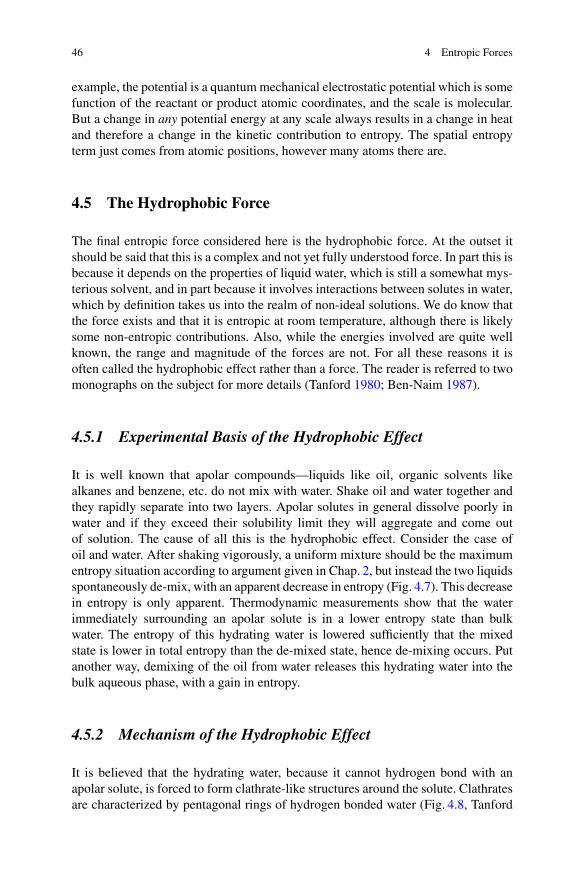
46 4 Entropic Forces
example, the potential is a quantum mechanical electrostatic potential which is somefunction of the reactant or product atomic coordinates, and the scale is molecular.But a change in any potential energy at any scale always results in a change in heatand therefore a change in the kinetic contribution to entropy. The spatial entropyterm just comes from atomic positions, however many atoms there are.
4.5 The Hydrophobic Force
The final entropic force considered here is the hydrophobic force. At the outset itshould be said that this is a complex and not yet fully understood force. In part this isbecause it depends on the properties of liquid water, which is still a somewhat mys-terious solvent, and in part because it involves interactions between solutes in water,which by definition takes us into the realm of non-ideal solutions. We do know thatthe force exists and that it is entropic at room temperature, although there is likelysome non-entropic contributions. Also, while the energies involved are quite wellknown, the range and magnitude of the forces are not. For all these reasons it isoften called the hydrophobic effect rather than a force. The reader is referred to twomonographs on the subject for more details (Tanford 1980; Ben-Naim 1987).
4.5.1 Experimental Basis of the Hydrophobic Effect
It is well known that apolar compounds—liquids like oil, organic solvents likealkanes and benzene, etc. do not mix with water. Shake oil and water together andthey rapidly separate into two layers. Apolar solutes in general dissolve poorly inwater and if they exceed their solubility limit they will aggregate and come outof solution. The cause of all this is the hydrophobic effect. Consider the case ofoil and water. After shaking vigorously, a uniform mixture should be the maximumentropy situation according to argument given in Chap. 2, but instead the two liquidsspontaneously de-mix, with an apparent decrease in entropy (Fig. 4.7). This decreasein entropy is only apparent. Thermodynamic measurements show that the waterimmediately surrounding an apolar solute is in a lower entropy state than bulkwater. The entropy of this hydrating water is lowered sufficiently that the mixedstate is lower in total entropy than the de-mixed state, hence de-mixing occurs. Putanother way, demixing of the oil from water releases this hydrating water into thebulk aqueous phase, with a gain in entropy.
4.5.2 Mechanism of the Hydrophobic Effect
It is believed that the hydrating water, because it cannot hydrogen bond with anapolar solute, is forced to form clathrate-like structures around the solute. Clathratesare characterized by pentagonal rings of hydrogen bonded water (Fig. 4.8, Tanford

4.5 The Hydrophobic Force 47
Fig. 4.7 Pentane and waterafter shaking (left), andde-mixing (right)
Fig. 4.8 Clathrate waterstructure around an apolargroup (partially hidden, inblack)
1980). The clathrate is more structured than bulk water. The positions and orien-tations of clathrate waters are more restricted. This reduces their spatial entropy.Following this line of argument, taking two separated apolar solute molecules andbringing them close enough to exclude water from their interface should result in anincrease in total entropy, since the amount of water in contact with apolar surface isdecreased. In going thus to a state of higher entropy, somewhere along this pathwaythere must be a positive gradient in entropy, and hence an attractive hydrophobicforce. This force presumably develops once the solute surfaces are close enoughexclude water, which is of the order of the diameter of a water molecule, ≈0.36 nm.This model predicts that the hydrophobic effect is proportional to the change inapolar surface area exposed to water. This area dependence is borne out quite wellby the data (Tanford 1980), which gives the change in water entropy per unit area ofabout −5.8 × 10⁻²³ J/K/nm2, which from Eq. 2.2 corresponds to about a 66-folddecrease in water spatial complexions per nm2. This gives a hydrophobic strength,defined as the free energy change per unit area exposed to water, of 104 J/mole/Å2.The magnitude of the hydrophobic effect is sufficient for it to play a major role inbiology: Helping to determine the structure and stability of proteins and promotingself assembly of biological membranes, for example.
While the structure of water around apolar molecules, especially large ones,may not be as regular as the clathrate model suggests the general concept of moreordered, lower entropy water hydrating apolar molecules is widely accepted as theorigin of the hydrophobic force.

48 4 Entropic Forces
SummaryThe maximum entropy state specifies what will be observed at equilibrium,which is basically a state with no net forces acting at the macroscopic level.Entropic effects can give rise to forces. These forces appear when a system isnot at equilibrium, or when part of a system is constrained from adoptingits maximum entropy state, for example a compressed gas or a stretchedrubber band. These forces are determined by the gradient in the spatial entropycontribution with respect to the pertinent displacement, e.g. a piston or the endof a polymer. Entropic forces are directed towards the maximum entropy stateand close to equilibrium they are typically linear in the displacement. Entropicforces are distinguished from forces arising from interaction potentials bytheir linear temperature dependence. By introducing the entropic potential−T S, forces from either entropic effects or interaction potentials can beobtained in the same way as the negative gradient of a potential with respectto the relevant displacement. When entropic forces and interaction potentialforces occur together, equilibrium may be described equivalently as
1. The state of maximum kinetic+spatial entropy2. The point of balance between all forces, from entropy and interaction
potentials3. The minimum in free energy, where the free energy is a sum of a spatial
entropy term multiplied by −T and a potential energy or enthalpy term.
Chapter 5Summary
Abstract Starting from the fact that atoms have both position and velocity, andusing basic concepts of mechanics—force, kinetic energy, potential energy and con-servation of energy—we have used complexion counting to obtain all the equationsrequired to understand both entropy and elementary statistical mechanics, includingfree energy. These are summarized here along with their physical meaning.
Keywords Boltzmann factor · Partition function · Free energy · Equilibriumconstant · Disorder
5.1 The Ubiquitous Boltzmann Factor
One mathematical factor appears over and over again in the discussion of entropyand statistical mechanics. It is the Boltzmann factor, which has the form
exp(X/kbT ) (5.1)
where X is some quantity with the units of energy, scaled by the mean kinetic energy(or temperature). It first appeared in Eq. 1.15 describing the increase in number ofvelocity complexions upon adding heat. It next appeared in Eq. 1.18 describing ther-mal equilibrium between two objects in contact. It appears as Eq. 1.25 describingthe probability of a particular spatial complexion. Most importantly, it appears asthe weighting term for each spatial complexion in the expression for the partitionfunction, Eq. 1.26. It appears as the factor describing the pressure distribution in theatmosphere (the Barometric equation 2.9). It appears in the Maxwell-Boltzmanndistribution of atomic velocities, Eq. 2.14. Finally, it appears in the expression forthe equilibrium constant, Eq. 3.19.
© The Author(s), under exclusive license to Springer Nature Switzerland AG 2019K. Sharp, Entropy and the Tao of Counting, SpringerBriefs in Physics,https://doi.org/10.1007/978-3-030-35457-2_5
49

50 5 Summary
5.2 The Important Equations
The first important equation is the sum of the Boltzmann factors over all the spatialcomplexions, also known as the partition function, Eq. 1.26:
Z =Ws∑i=1
exp(−Ui/kbT )
This quantity is central to statistical mechanics. This not surprising since, as Eq. 1.31tells us, it is to within a multiplicative constant just the total number of complexions
W = C′Z
The Boltzmann factor itself, Eq. 1.25,
pi = exp(−Ui/kbT )
Z
gives us the probability of each spatial complexion. From this it is possible tocalculate many average, or macroscopic, properties by forming their probabilityweighted sum over the spatial complexions.
The entropy is, to within an additive constant, the logarithm of the total numberof complexions. The entropy change given by Eq. 2.4 is thus the difference in thelogarithm of the total number of complexions
ΔS = kb(lnW ′ − lnW)
For the special case of an ideal gas, the total number of complexions is just theproduct of the number of spatial complexions and kinetic energy complexions(Eq. 1.21). The former is proportional to the volume raised to the power of thenumber of atoms, V N , while the latter is proportional to the total kinetic energyraised the power of 3N/2, namely E
3N/2K . This separability leads to a simple additive
formula for the ideal gas entropy, Eq. 2.7
Sid = NkblnV + 3
2NkblnT + C
The partition function can be used to obtain one of the most important averagequantities, the mean potential energy, Eq. 1.28
U = 1
Z
Ws∑i=1
Uiexp(−Ui/kbT )

5.4 Modest Entropies but Very Very Large Numbers 51
The logarithm of the partition function (difference) yields a free energy (difference).For constant pressure conditions, this is the Gibb’s free energy, Eq. 3.14:
ΔG = −kbT ΔlnZ = ΔH − T ΔSs
where ΔH = ΔU + PΔV is the change in heat (kinetic energy) resulting fromthe change in potential energy minus any pressure-volume work done. It should beremembered that the free energy change here is simply −T times the total entropychange, which itself consists of a kinetic energy contribution, ΔSv = −ΔH/T , anda spatial contribution, ΔSs .
Finally, an important experimental quantity, the equilibrium constant, is alsorelated to the free energy difference by Eq. 3.19:
KAB = exp(−ΔGAB/kbT )
5.3 What About Quantum Mechanics?
The treatment here uses classical mechanics only. Yet the real world obeys the rulesof quantum mechanics. How does this change things? The answer is very little. First,Boltzmann’s postulate still applies: All possible complexions (read quantum states)with a given number of atoms and total energy are equally likely (Tolman 1938). Thedefinition of entropy as a logarithmic measure of the number of complexions stillapplies. Only the counting of complexions is affected by quantization. However,all the applications here involve large numbers of atoms at normal temperatures.Under these conditions, the number of quantum states is so vast and their energylevels so close together that the classical treatment of counting given here is morethan adequate. The Boltzmann distribution is closely followed and the macroscopic,thermodynamic behavior is accurately described. Generally speaking, a quantummechanical treatment is only necessary when studying a very small number ofatoms, very low temperatures or the interaction of radiation with atoms.
5.4 Modest Entropies but Very Very Large Numbers
The machinery for complexion counting was applied to several everyday events.We now give both the change in number of complexions and the change in entropy,using Eq. 2.4
1. Heat flows from hot to cold. Temperature equilibration of two 0.1 kg blocks ofcopper differing in temperature by 1 millionth of a degree:
W ′
W≈ 103,400,000 ΔS ≈ 1 × 10⁻¹⁶ J/K

52 5 Summary
2. A moving object comes to rest due to friction. For a 0.1 kg ball falling 0.1 m:
W ′
W≈ 101019
ΔS ≈ 0.33 mJ/K
3. A gas expands into the available volume. For 10 cc of gas expanding to twice itsvolume:
W ′
W≈ 101020
ΔS ≈ 2.6 mJ/K
4. A gas-cylinder spring of cross-sectional area 0.01 m2 is loaded with a 4 kg weight
W ′
W≈ 101.4×10¹⁹
ΔS ≈ 0.43 mJ/K
5.5 Different Interpretations of Entropy
From its inception, entropy has been given a surprising variety of physical inter-pretations. The most common are discussed here in the context of the method ofcomplexion counting described in this book.
5.5.1 Entropy as Disorder
Most of the pioneers in the development of statistical mechanics have at some timeequated an increase in entropy with an increase in disorder. A completely non-technical but remarkably accurate description of entropy as disorder is providedby the anthropologist Gregory Bateson in a charming fictional dialogue with hisdaughter (Bateson 1972). Nevertheless, some care is required with this definitionto avoid apparent contradictions. Take for example supercooled liquid water. Beinga liquid, its molecular structure is quite disordered. Thermodynamic equilibrium isreached when the water freezes. Now the molecules are more ordered spatially as icecrystals. Yet this spontaneous process must have an overall increase in entropy. Thecontradiction is only apparent. When water freezes there is a positive latent heatof fusion which causes an increase in velocity complexions. Because the spatialcomponent is literally the only part of the entropy change that is visible, it is easyto assume that it is the only part. This illustrates the limitation, alluded to in theintroduction, of popular explanations of entropy that discuss only the spatial contri-bution, not the kinetic part. The latter, invisible, contribution must be included usingBoltzmann’s equation 1.15. The overall amount of disorder, spatial plus kinetic,does increase and the entropy change provides a quantitative measure of this.
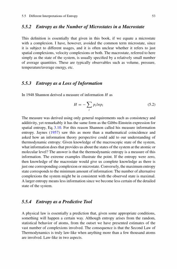
5.5 Different Interpretations of Entropy 53
5.5.2 Entropy as the Number of Microstates in a Macrostate
This definition is essentially that given in this book, if we equate a microstatewith a complexion. I have, however, avoided the common term microstate, sinceit is subject to different usages, and it is often unclear whether it refers to justspatial complexions, velocity complexions or both. The macrostate, referred to heresimply as the state of the system, is usually specified by a relatively small numberof average quantities. These are typically observables such as volume, pressure,temperature/average energy, etc.
5.5.3 Entropy as a Loss of Information
In 1948 Shannon derived a measure of information H as
H = −∑
i
pi lnpi (5.2)
The measure was derived using only general requirements such as consistency andadditivity, yet remarkably it has the same form as the Gibbs-Einstein expression forspatial entropy, Eq. 3.10. For this reason Shannon called his measure informationentropy. Jaynes (1957) saw this as more than a mathematical coincidence andasked how an information theory perspective could add to our understanding ofthermodynamic entropy: Given knowledge of the macroscopic state of the system,what information does that provides us about the states of the system at the atomic ormolecular level? The answer is that the thermodynamic entropy is a measure of thisinformation. The extreme examples illustrate the point. If the entropy were zero,then knowledge of the macrostate would give us complete knowledge as there isjust one corresponding complexion or microstate. Conversely, the maximum entropystate corresponds to the minimum amount of information: The number of alternativecomplexions the system might be in consistent with the observed state is maximal.A larger entropy means less information since we become less certain of the detailedstate of the system.
5.5.4 Entropy as a Predictive Tool
A physical law is essentially a prediction that, given some appropriate conditions,something will happen a certain way. Although entropy arises from the random,statistical behavior of atoms, from the outset we have presented estimates of thevast number of complexions involved. The consequence is that the Second Law ofThermodynamics is truly law-like when anything more than a few thousand atomsare involved. Law-like in two aspects.

54 5 Summary
First, equilibrium behavior can with almost no error be predicted from theproperties of the macrostate with the most complexions. Even if the system neversamples that particular set of complexions it will with almost certainty sample onlythose indistinguishable from it. Here there is no requirement for ergodicity. Becauseof the vast numbers of complexions involved, the statistical limit to the accuracy ofpredictions about observable states and thermodynamic equilibria is better than thatof most measuring instruments. The accuracy is in fact as good as, or better than,predictions of physical behaviors governed by non-statistical laws such as those ofelectromagnetism or classical dynamics.
Second, we can predict with almost certainty that a non-equilibrium system willchange in such a way as to increase its entropy. In fact, provided the system isnot too far from equilibrium the gradient of the entropy provides the forces, andhence the pathway of change. The famous tension between the time-reversibility offundamental physical laws and the irreversibility of the Second Law was resolved, inBoltzmann’s time, by recognizing the crucial role of initial conditions (Boltzmann1895). Tracing the origins of lower entropy back further and further in time,the source of the time asymmetry that sets the direction for the Second Law iscosmological (Davies 1977). For reasons that are yet unclear, the universe startedoff in a very low entropy state because of the uniformity of the gravitational field,and it has been running uphill in entropy ever since.
5.5.5 Entropy as the Number of Ways Something Can Happen
The theme of this book is that entropy is simply a logarithmic measure of thenumber of ways the positions and velocities of the atoms can be arranged consistentwith a given macroscopic, observable state. The corollary is: what we see iswhat can happen the most ways, what has the largest entropy. Even a very tinyentropy increase corresponds to truly huge increase in the number of complexions,ineluctably orienting the arrow of time we experience every day.

Appendix
A.1 The Exponential and Logarithm Functions
Aside from standard algebra, the only other mathematics used in this book involvesthe exponential and logarithm functions. Their basic properties are summarizedhere.
The exponential function, base-10, is written as y = 10x , where x is theexponent. This is familiar from common notation used for large decimal numbers.For example
101 = 10, 102 = 100, 103 = 1000, etc. (A.1)
although the exponent need not be an integer. If two exponentials of the same baseare multiplied/divided, their exponents are added/subtracted:
10c × 10d = 10(c+d), 10c/10d = 10(c−d) (A.2)
The logarithm function is simply the inverse of the exponential function:
y = 10x ⇒ x = log10(y) or y = 10log10(y). (A.3)
Adding/subtracting logarithms multiplies/divides their arguments:
log10(c) + log10(d) = log10(c × d) (A.4)
log10(c) − log10(d) = log10(c/d) (A.5)
Repeated application of the addition rule for the same number c gives the power rule
log10(cn) = n log10(c) (A.6)
© The Author(s), under exclusive license to Springer Nature Switzerland AG 2019K. Sharp, Entropy and the Tao of Counting, SpringerBriefs in Physics,https://doi.org/10.1007/978-3-030-35457-2
55

56 Appendix
Base-10 is useful for expressing large numbers in a comprehensible manner: Theexponent simply describes how many zeros follow the 1 in decimal notation.However the natural base for exponential functions (because of its more convenientmathematical properties) is Euler’s number e = 2.71828 . . .. An exponential in thisbase is simply written as ex . The corresponding logarithm to base e, known as thenatural logarithm, is written as ln(x). The rule for converting exponents betweenbases 10 and e is
ex = 10x/ln(10) (A.7)
where ln(10) = 2.303 . . .. The corresponding rule for converting logarithmsbetween bases 10 and e is
ln(x) = ln(10) × log10(x) (A.8)
Exponents and logarithms in the natural base follow all the same rules as for base-10.
ec × ed = e(c+d) (A.9)
y = ex ⇒ x = ln(y) or y = eln(y) (A.10)
ln(c) + ln(d) = ln(c × d) (A.11)
ln(cn) = n ln(c) (A.12)
A useful approximation for the natural logarithm when the argument is close to 1 is:
ln(1 + x) ≈ x (x 1) (A.13)
For example, when x = 0.01, ln(1 + x) = 0.00995 with less than half a percenterror. For smaller values of x encountered here, the approximation is effectivelyerror-less.
A.2 Mechanical Origins of the Ideal Gas Law
To round out the mechanical presentation of statistical mechanics the ideal gaslaw, also known as Boyle’s law, is derived using basic mechanical concepts. Thisalso provides the relationship between the mean kinetic energy of the atomsand temperature required in Sect. 1.2. Consider a rectangular box of volume V
containing N molecules of an ideal gas. The molecules of the gas will continuallybe colliding with the walls of the box and rebounding. These collisions produce a

A.2 Mechanical Origins of the Ideal Gas Law 57
Fig. A.1 Origin of the idealgas law
force on the walls given by the rate of change of momentum of the gas molecules.The pressure exerted by the gas is just the average force per unit area. Consider themolecules colliding with the right hand wall of the box (Fig. A.1). The area of thewall is A. If in a short time dt a number of molecules b with mass m and velocityu in the x direction collide with the wall, then the change in momentum is 2mub.There’s a factor of two because the collision reverses the velocity in the x direction.The pressure is the rate of change of momentum per unit area
P = 2mub
Adt(A.14)
The number of molecules b that collide with the wall in time dt is equal to thenumber of molecules within a distance dx = udt of the wall that are movingtowards the wall, namely with a positive velocity in the x-direction. This is half thetotal number of molecules in a volume Adx, since on average half the moleculeswill be moving to the right, and half to the left. The gas density is N/V , sob = NAdx/2V . Substituting for dx the number of collisions is
b = NAdtu
2V(A.15)
Substituting for b in Eq. A.14, the pressure is
P = Nmu2
V(A.16)
Finally, since there will be a range of velocities, u2 in Eq. A.16 must be replaced by
the mean squared velocity, u2. This is obtained from the expression for the meankinetic energy of the molecules, Eq. 1.4:
EK = m
2N
N∑i
(u2i + v2
i + w2i ) = m
2(u2 + v2 + w2) (A.17)

58 Appendix
Now the mean squared velocities in the x, y and z directions will be the same sincethe gas is homogeneous and at equilibrium. So
u2 = v2 = w2 = 2EK
3m. (A.18)
Using this expression for u2 in Eq. A.16 we obtain the ideal gas law
PV = N2
3EK (A.19)
in terms of the mean kinetic energy. P , V and T had previously been measured forvarious gases leading to the empirical Boyle’s Law
PV = nRT = NkbT (A.20)
where n is the number of moles of gas and R = 8.314 J/K/mole is the gas constant.The second form of Boyle’s Law uses the fact that the number of molecules in n
moles is given by N = Nan where Na = 6.02 × 10²³ is Avogadro’s number. Sothe scale factor relating temperature, measured on the ideal gas or Kelvin scale, andmean kinetic energy per molecule is
2
3EK = kbT (A.21)
where Boltzmann’s constant kb = R/Na has a value of 1.38 × 10⁻²³ J/K.

References
Bateson G (1972) Metalogue: why do things get in a Muddle? In: Steps to an ecology of mind.Ballantine Books, New York
Ben-Naim A (1987) Solvation thermodynamics. Plenum Press, New YorkBiot MA (1955) Variational principles in irreversible thermodynamics with application to vis-
coelasticity. Phys Rev 97:1463–1469Boltzmann L (1877) Uber die Beziehung zwischen dem zweiten Hauptsatze der mechanischen
Warmetheorie und der Wahrscheinlichkeitsrechnung respektive den Satzen uber das Warmgle-ichgewicht. Weiner Berichte 76:373–435
Boltzmann L (1895) On certain questions of the theory of gases. Nature 51:413–415Bridgman PW (1972) The nature of thermodynamics. Harper and Brothers, New YorkCraig NC (2005) Let’s drive “driving force” out of chemistry. J Chem Educ 82:827Davies PCW (1977) The physics of time asymmetry. Surrey University Press, LondonFeynman RP (1972) Statistical mechanics; a set of lectures. W.A. Benjamin, ReadingJaynes ET (1957) Information theory and statistical mechanics. Phys Rev 106:620–630Shannon CE (1948) A mathematical theory of communication. Bell Syst Tech J 27:379–423Sharp KA, Matschinsky F (2015) Translation of Ludwig Boltzmann’s paper “On the Relationship
between the Second Fundamental Theorem of the Mechanical Theory of Heat and ProbabilityCalculations Regarding the Conditions for Thermal Equilibrium” (Wien. Ber. 1877, 76:373–435). Entropy 17:1971–2009
Tanford C (1961) Physical chemistry of macromolecules. Wiley, New YorkTanford C (1980) The hydrophobic effect, 2nd edn. Wiley, New YorkTolman RC (1938) The principles of statistical mechanics. Clarendon Press, Oxford
© The Author(s), under exclusive license to Springer Nature Switzerland AG 2019K. Sharp, Entropy and the Tao of Counting, SpringerBriefs in Physics,https://doi.org/10.1007/978-3-030-35457-2
59

Index
AAtom
complexion, 4–5equilibrium distribution, 21force on, 37kinetic energy, 3probability, 26velocity, 2–3
Avogadro’s number, 23, 58
BBarometric equation, 24, 49Boltzmann factor, 16, 49, 50Boltzmann’s constant, 4, 58Boltzmann’s equation, 10–12, 52Boltzmann’s postulate, 5–6, 22, 26Boyle’s Law, 39, 56, 58
CComplexion, 1–2
accounting atoms, masses, 9Boltzmann’s equation, 10constant temperature conditions, 17heat effect, velocity, 8–9kinetic energy, 7, 11single atom, 6spatial and velocity, 14total number, 16–17velocity, 6
EEnthalpy, 32, 42, 45Entropic force
in gas, 38–43polymers, 43–45potential energy, 37–38
Entropic work, 31, 32, 40, 51Entropy
Boltzmann’s expression, 20dice analogy, 20disorder, 52equilibrium behavior, 54equilibrium constants, 32–34factorial functions, 21and free energy (see Free energy)gas molecules, 21, 22Gibbs–Einstein equation, 30–31ideal gas, 23information, measurement, 53kinetic energy, 19, 30language of energetics, 32macroscopic quantities, 20microstate, 53non-equilibrium system, 54partition function, 29physical law, 53positions and velocities, atoms, 54potential energy, 30solute, 22spatial complexions, 29spatial contribution, 30surface free energy work, 31
© The Author(s), under exclusive license to Springer Nature Switzerland AG 2019K. Sharp, Entropy and the Tao of Counting, SpringerBriefs in Physics,https://doi.org/10.1007/978-3-030-35457-2
61
62 Index
Entropy (cont.,)temperature, 20thermodynamic, 19
Entropy derivative, 41Equilibrium
entropy, 20–22thermal, 11velocity-sphere concept, 24
Equilibrium constants, 51chemical reaction, 34complexions, 33entropy, 34solute, solvents, 32thermodynamic relationship, 33
Evaporative cooling, 27Exponential and logarithm functions, 55–56
FForce
Hydrophobic force (see Hydrophobicforce)
See also Entropic forceFree energy
entropy (see Entropy)Gibb’s free energy, 51
Friction, 12–13, 52
GGas molecule, 24Gibbs–Einstein equation, 30–31, 53
HHooke’s law, 38, 44, 45Hydrophobic force, 46, 47
clathrate water structure, 47, 48experimental basis, 46mechanism, 46–47
IIdeal gas, 23
atmosphere, 41cylindrical piston, 39entropic forces, 38entropy contribution, 41equilibrium position, 39–40free energy expression, 42IP-forces, 39mean squared velocities, 57–58
origin, 56–57statistical mechanics, 56
KKelvin scale, 58Kinetic energy, 2
of atom, 3–4complexions, 11components, 26equilibrium distribution, 24probability, 27
MMaxwell–Boltzmann distribution, 27, 28, 49
NNewton’s Third Law, 14
OOsmotic pressure, 42–43
PPartition function, 16, 17, 29, 50
logarithm, 51Polymers
elastic cord, 44–45end-to-end distance, 43–44gravitational and elastic force balance, 45rigid segments, 43
Potential energy, 14–16and forces, 37–38gas molecule, 24gravitational, 44
Pythagoras’ theorem, 2, 6
QQuantum mechanics, 46, 51
SSpatial and velocity complexions
Boltzmann factor, 16energy atoms, 14–15potential energy, 15velocity, 14

Index 63
TTemperature, 10–12, 17, 23, 24, 27, 30, 31, 39,
51, 53
VVelocity
atomcomponent, 25kinetic energy, 25
chemical and biochemical reactions,27–28
complexion, 4component, 6, 26evaporative cooling, 27heat effect, 8sphere, 7, 10, 15vectors, 63N-dimensional vector, 7