keysight technologies comparison of different jitter analysis...

Keysight TechnologiesComparison of Different Jitter Analysis Techniques With a Precision Jitter Transmitter

White Paper

02 | Keysight | Comparison of Different Jitter Analysis Techniques With a Precision Jitter Transmitter – White Paper

DesignCon - February 2, 2005Ransom Stephens, Brian Fetz, Steve Draving, Joe Evangelista, Michael Fleischer-Reu-mann, Greg LeCheminant, Jim Stimple

Different jitter analysis techniques yield results that can vary by hundreds of percent.

At Keysight Technologies, Inc. we were aware of the discrepancies and invested into the research necessary to understand the situation before introducing a solution. We built a data transmitter with a complete set of applied jitter levels precisely calibrated, in most cases, to traceable standards1. We assembled jitter analysis equipment, three 6 GHz bandwidth real-time oscilloscopes and a 4 GHz bandwidth time interval analyzer, from the major vendors as well as a Keysight bit error ratio tester (N4901B SerialBERT) and a Digital Communication Analyzer (86100C DCA-J) equipped with a 20 GHz electrical re-ceiver and then applied a wide variety of signals with known TJ(10–12) and known levels of different types of jitter to determined which analyzers are accurate and why.

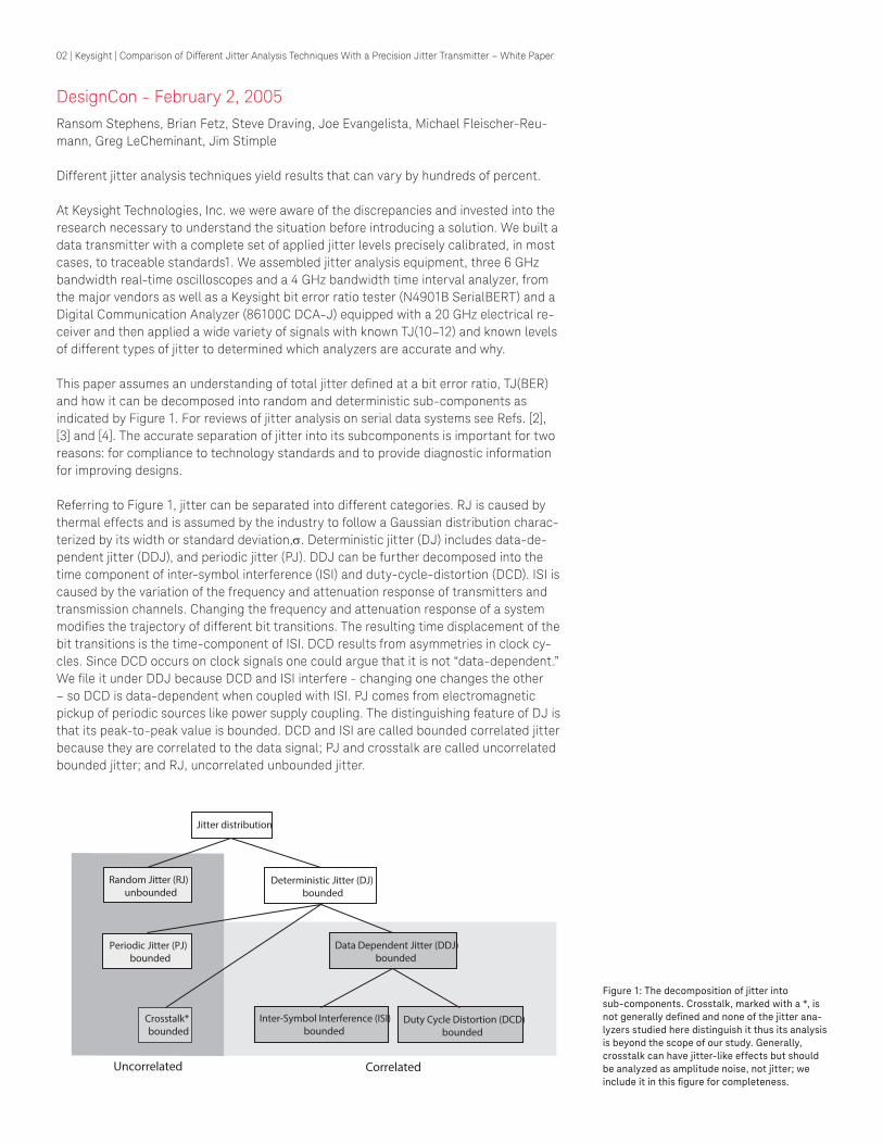
This paper assumes an understanding of total jitter defined at a bit error ratio, TJ(BER) and how it can be decomposed into random and deterministic sub-components as indicated by Figure 1. For reviews of jitter analysis on serial data systems see Refs. [2], [3] and [4]. The accurate separation of jitter into its subcomponents is important for two reasons: for compliance to technology standards and to provide diagnostic information for improving designs.

Referring to Figure 1, jitter can be separated into different categories. RJ is caused by thermal effects and is assumed by the industry to follow a Gaussian distribution charac-terized by its width or standard deviation,σ. Deterministic jitter (DJ) includes data-de-pendent jitter (DDJ), and periodic jitter (PJ). DDJ can be further decomposed into the time component of inter-symbol interference (ISI) and duty-cycle-distortion (DCD). ISI is caused by the variation of the frequency and attenuation response of transmitters and transmission channels. Changing the frequency and attenuation response of a system modifies the trajectory of different bit transitions. The resulting time displacement of the bit transitions is the time-component of ISI. DCD results from asymmetries in clock cy-cles. Since DCD occurs on clock signals one could argue that it is not “data-dependent.” We file it under DDJ because DCD and ISI interfere - changing one changes the other – so DCD is data-dependent when coupled with ISI. PJ comes from electromagnetic pickup of periodic sources like power supply coupling. The distinguishing feature of DJ is that its peak-to-peak value is bounded. DCD and ISI are called bounded correlated jitter because they are correlated to the data signal; PJ and crosstalk are called uncorrelated bounded jitter; and RJ, uncorrelated unbounded jitter.

Figure 1: The decomposition of jitter into sub-components. Crosstalk, marked with a *, is not generally defined and none of the jitter ana-lyzers studied here distinguish it thus its analysis is beyond the scope of our study. Generally, crosstalk can have jitter-like effects but should be analyzed as amplitude noise, not jitter; we include it in this figure for completeness.

CorrelatedUncorrelated

Periodic Jitter (PJ)bounded

Deterministic Jitter (DJ)bounded

Data Dependent Jitter (DDJ)bounded

Inter-Symbol Interference (ISI)bounded

Duty Cycle Distortion (DCD)bounded

Crosstalk*bounded

Random Jitter (RJ)unbounded

Jitter distribution


1. Jitter Test Results Are All Over The Map

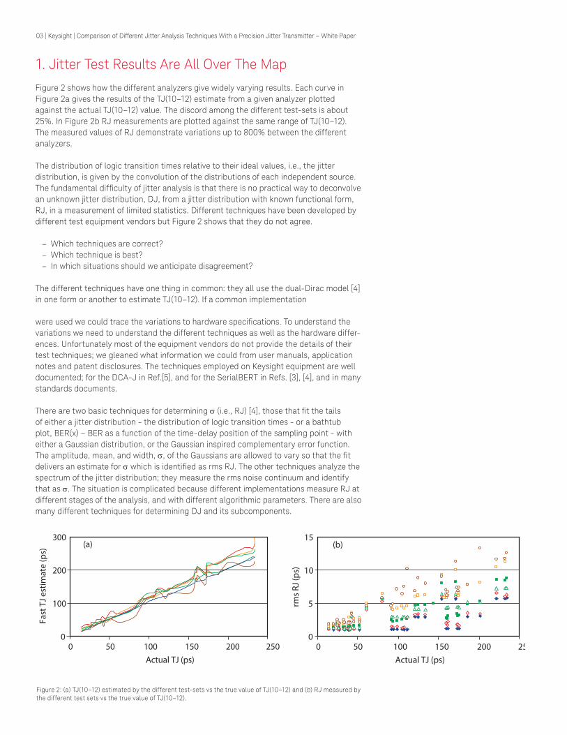
Figure 2 shows how the different analyzers give widely varying results. Each curve in Figure 2a gives the results of the TJ(10–12) estimate from a given analyzer plottedagainst the actual TJ(10–12) value. The discord among the different test-sets is about 25%. In Figure 2b RJ measurements are plotted against the same range of TJ(10–12). The measured values of RJ demonstrate variations up to 800% between the different analyzers.

The distribution of logic transition times relative to their ideal values, i.e., the jitter distribution, is given by the convolution of the distributions of each independent source. The fundamental difficulty of jitter analysis is that there is no practical way to deconvolve an unknown jitter distribution, DJ, from a jitter distribution with known functional form, RJ, in a measurement of limited statistics. Different techniques have been developed by different test equipment vendors but Figure 2 shows that they do not agree.

– Which techniques are correct? – Which technique is best? – In which situations should we anticipate disagreement?

The different techniques have one thing in common: they all use the dual-Dirac model [4] in one form or another to estimate TJ(10–12). If a common implementation

were used we could trace the variations to hardware specifications. To understand the variations we need to understand the different techniques as well as the hardware differ-ences. Unfortunately most of the equipment vendors do not provide the details of theirtest techniques; we gleaned what information we could from user manuals, application notes and patent disclosures. The techniques employed on Keysight equipment are well documented; for the DCA-J in Ref.[5], and for the SerialBERT in Refs. [3], [4], and in many standards documents.

There are two basic techniques for determining σ (i.e., RJ) [4], those that fit the tails of either a jitter distribution - the distribution of logic transition times - or a bathtub plot, BER(x) – BER as a function of the time-delay position of the sampling point - with either a Gaussian distribution, or the Gaussian inspired complementary error function. The amplitude, mean, and width, σ, of the Gaussians are allowed to vary so that the fit delivers an estimate for σ which is identified as rms RJ. The other techniques analyze the spectrum of the jitter distribution; they measure the rms noise continuum and identify that as σ. The situation is complicated because different implementations measure RJ at different stages of the analysis, and with different algorithmic parameters. There are also many different techniques for determining DJ and its subcomponents.

Figure 2: (a) TJ(10–12) estimated by the different test-sets vs the true value of TJ(10–12) and (b) RJ measured by the different test sets vs the true value of TJ(10–12).

15

10

5

00 50 100 150 200 250

Actual TJ (ps)

rms R

J (ps

)

300

200

100

00 50 100 150 200 250

Actual TJ (ps)

Fast

TJ e

stim

ate

(ps)

(a) (b)


2. How To Compare Different Techniques

Prior to our study, jitter test-system designers developed their algorithms with three tools: first, evaluation of their algorithms in simulations; second, testing with calibrated levels of sinusoidal PJ using the well established techniques from SONET/SDH [6]; and, third, by comparing their TJ(BER) estimates with measurements performed on a BERT (note: be careful to distinguish between a complete measurement of TJ(BER) on a BERT [7], and a fast estimate of TJ(BER) on a BERT [3]). None of these methods challenge the test-sets with real jitter conditions at known levels - so we built a precision jitter trans-mitter that does.

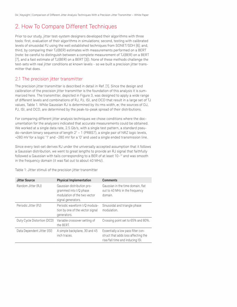
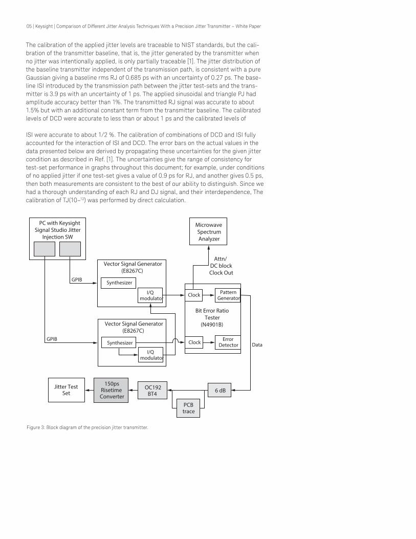
2.1 The precision jitter transmitterThe precision jitter transmitter is described in detail in Ref. [1]. Since the design and calibration of the precision jitter transmitter is the foundation of this analysis it is sum-marized here. The transmitter, depicted in Figure 3, was designed to apply a wide range of different levels and combinations of RJ, PJ, ISI, and DCD that result in a large set of TJ values, Table 1. While Gaussian RJ is determined by its rms width, σ; the sources of DJ, PJ, ISI, and DCD, are determined by the peak-to-peak spread of their distributions.

For comparing different jitter analysis techniques we chose conditions where the doc-umentation for the analyzers indicated that accurate measurements could be obtained. We worked at a single data rate, 2.5 Gb/s, with a single test pattern, a standard pseu-do-random binary sequence of length 27 – 1 (PRBS7), a single pair of NRZ logic levels, +280 mV for a logic ‘1’ and –280 mV for a ‘0’ and used a single ended transmission line.

Since every test-set derives RJ under the universally accepted assumption that it follows a Gaussian distribution, we went to great lengths to provide an RJ signal that faithfully followed a Gaussian with tails corresponding to a BER of at least 10–12 and was smooth in the frequency domain (it was flat out to about 40 MHz).

Table 1: Jitter stimuli of the precision jitter transmitter

Jitter Source Physical Implementation Comments

Random Jitter (RJ) Gaussian distribution pro-grammed into I/Q phase modulation of the two vector signal generators.

Gaussian in the time domain, flat out to 40 MHz in the frequency domain.

Periodic Jitter (PJ) Periodic waveform I/Q modula-tion by one of the vector signal generators.

Sinusoidal and triangle phase modulation.

Duty Cycle Distortion (DCD) Variable crossover setting of the BERT.

Crossing point set to 65% and 80%.

Data Dependent Jitter (ISI) A simple backplane, 30 and 45 inch traces.

Essentially a low pass filter con-struct that adds loss affecting the rise/fall time and inducing ISI.


The calibration of the applied jitter levels are traceable to NIST standards, but the cali-bration of the transmitter baseline, that is, the jitter generated by the transmitter when no jitter was intentionally applied, is only partially traceable [1]. The jitter distribution of the baseline transmitter independent of the transmission path, is consistent with a pure Gaussian giving a baseline rms RJ of 0.685 ps with an uncertainty of 0.27 ps. The base-line ISI introduced by the transmission path between the jitter test-sets and the trans-mitter is 3.9 ps with an uncertainty of 1 ps. The applied sinusoidal and triangle PJ had amplitude accuracy better than 1%. The transmitted RJ signal was accurate to about 1.5% but with an additional constant term from the transmitter baseline. The calibrated levels of DCD were accurate to less than or about 1 ps and the calibrated levels of

ISI were accurate to about 1/2 %. The calibration of combinations of DCD and ISI fully accounted for the interaction of ISI and DCD. The error bars on the actual values in the data presented below are derived by propagating these uncertainties for the given jitter condition as described in Ref. [1]. The uncertainties give the range of consistency for test-set performance in graphs throughout this document; for example, under conditions of no applied jitter if one test-set gives a value of 0.9 ps for RJ, and another gives 0.5 ps, then both measurements are consistent to the best of our ability to distinguish. Since we had a thorough understanding of each RJ and DJ signal, and their interdependence, The calibration of TJ(10–12) was performed by direct calculation.

Figure 3: Block diagram of the precision jitter transmitter.

MicrowaveSpectrumAnalyzer

Jitter TestSet

PCBtrace

6 dBOC192BT4

150psRisetimeConverter

Vector Signal Generator(E8267C)

Synthesizer

I/Qmodulator

Vector Signal Generator(E8267C)

Synthesizer

I/Qmodulator

PC with KeysightSignal Studio Jitter

Injection SW

Bit Error RatioTester

(N4901B)

Clock PatternGenerator

ErrorDetectorClock

Attn/DC blockClock Out

Data

GPIB

GPIB


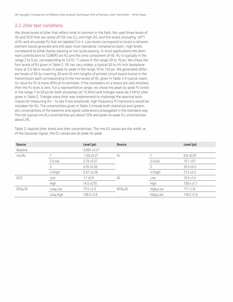
2.2 Jitter test conditionsWe chose levels of jitter that reflect what is common in the field. We used three levels of ISI and DCD that we called off (O), low (L), and high (H), and five levels (including “off”) of RJ and sinusoidal PJ that we labeled 0 to 4. Low levels correspond to levels a network element would generate and still pass most standards’ compliance tests. High levels correspond to either barely passing or not quite passing. In most applications the domi-nant contributors to TJ(BER) are RJ and the time component of ISI. RJ is typically in the range 2 to 5 ps, corresponding to TJ(10–12) values in the range 28 to 70 ps. We chose the four levels of RJ given in Table 2. ISI can vary widely; a typical 30 to 45 inch backplane trace at 2.5 Gb/s results in peak-to-peak in the range 70 to 140 ps. We generated differ-ent levels of ISI by inserting 30 and 45 inch lengths of printed circuit board traces in the transmission path corresponding to the two levels of ISI, given in Table 2 A typical realis-tic value for PJ is more difficult to estimate. If the oscillators on a board are well shielded, then the PJ level is zero. For a representative range, we chose the peak-to-peak PJ levels in the range 7 to 28 ps for both sinusoidal (at 15 MHz) and triangle-wave (at 2 MHz) jitter given in Table 2. Triangle wave jitter was implemented to challenge the spectral tech-niques for measuring RJ – to see if low amplitude, high frequency PJ harmonics would be mistaken for RJ. The uncertainties given in Table 2 include both statistical and system-atic uncertainties of the baseline and signal calibrations propagated in the standard way. The net typical rms RJ uncertainties are about 10% and peak-to-peak DJ uncertainties about 2%.

Table 2: Applied jitter levels and their uncertainties. The rms RJ values are the width, σ,of the Gaussian signal, the DJ values are all peak-to-peak.

Source Level (ps) Source Level (ps)

Baseline 0.685 ±0.27

rms RJ 1 1.39 ±0.27 PJ 1 6.8 ±0.07

2 (Low) 2.79 ±0.27 2 (Low) 13.7 ±0.1

3 4.18 ±0.28 3 20.5 ±0.2

4 (High) 5.57 ±0.28 4 (High) 27.3 ±0.3

DCD Low 7.7 ±0.9 ISI Low 70.5 ±1.4

High 14.0 ±0.15 High 139.4 ±1.7

DCD*ISI Low*Low 72.5 ±2.3 DCD*ISI High*Low 77.1 ±1.6

Low*High 138.5 ±2.6 High*Low 140.5 ±1.9


2.3 Set up of the jitter analyzersTo maintain a level playing field the test-sets were configured under two criteria. First, the configurations were designed so that the different test sets should give the same re-sults. For example, they were configured to measure the full jitter-frequency bandwidth. Since all jitter measurements can be reduced to the comparison of a test clock and a reference clock [2], the unmodulated system clock was used on those test-sets that accepted a system clock and, in those cases that didn’t, the reconstructed clock was set with the lowest bandwidth possible.

Second, the analyzers were configured using minimal modifications to the default settings and a single configuration was used for all test cases. The idea was to set up the equipment the way that most engineers would. We used the settings that the user manuals indicated would give the best results and allowed for longer test times to accommodate the manufacturers’ suggestions for increased accuracy. The duration of measurements varied from less than ten seconds for one of the real-time oscilloscopes to over a minute for another.

The Keysight DCA-J is pre-configured requiring no set-up and required less than ten seconds to perform the measurements reported here.

The SerialBERT was configured to transmit until either 3x109 bits were sent or 1000 errors counted – whichever came first – in 1 ps increments of the time-delay setting. The BER threshold was set at 10–4, below which the simple fitting implementation of the dual-Dirac model was applied.

Comment on commercial competition: It’s easy to speculate that a group of Keysight engineers might set up their competitor’s equipment to give poor results. This study was originally an internal evaluation of the state of jitter analysis. Since we only had the equipment for one week, we had to set up the competitive equipment the way that the users’ manual recommended and get the best measurements we could as quickly as possible to cover a representative set of jitter conditions. On the other hand, our time limitations constrained us to testing only one of the techniques available on each system. We chose the technique the manufacturer recommended, regardless of test duration.

Figure 4: (a) TJ(10–12) estimated by the different test-sets vs the true value (white line), and (b) the percent error in the estimated values –that is, the percent deviation between the estimate and the true value.

0 50 100 150 200 250Actual TJ (ps)

60

40

20

0

–20

–40

Frac

tiona

l Err

or in

TJ (

%)

(b)

0 50 100 150 200 250Actual TJ (ps)

300

225

150

75

0

Frac

tiona

l Err

or in

TJ (

%)

(a)

TJ error

TJ estimate vs actual TJ

True valuesKeysight 86100C DCA-JKeysight N4901B SerialBERT6 GHz real-time oscilloscope – X6 GHz real-time oscilloscope – Y6 GHz real-time oscilloscope – Z4 GHz time interval analyzer


3. Comparison Of Different Techniques

Figure 4 gives the same data as Figure 2a, estimated TJ(10–12) vs the true value, but including the actual values (the white curve). The Keysight jitter analyzers, the DCA-J(solid blue diamonds) and SerialBERT (solid green squares), are labeled. The other data points are the results from jitter analyzers produced by companies other than Keysight Technologies. They include real-time oscilloscopes and time interval analyzers. Figure 4b gives the fractional error of the TJ(10–12) estimates; that is, the difference of the esti-mate and truth divided by the true value. The error bars in Figure 4b indicate the calibra-tion uncertainty in the true values – any measurement within the vertical span should be considered consistent with the truth. As TJ(10–12) increases, the jitter conditions grow more complex. All the test-sets do well on the left with simple conditions but as more combinations of RJ, PJ, ISI, and DCD are introduced the errors increase.

Figure 5, has the same data as Figure 2b, measured RJ vs TJ(10–12), but including the true RJ values and their uncertainties. The deviation from measured and true RJ in simple jitter conditions are small, but for complex conditions most of the analyzers are inaccurate by between 100% and 500%. We’ll see below that the discrepancy is domi-nated by analyzers whose RJ measurements are affected by the introduction of DDJ.

The fast SerialBERT TJ(10–12) estimates in Figure 4 are mostly consistent with the true values of TJ(10–12), but are less consistent with RJ, in Figure 5. The SerialBERT technique is a straightforward fitting application of the dual-Dirac model makes quite accurate fast estimates of TJ(10–12) but is not as accurate as the DCA-J in resolving the subcomponents. The strength of jitter analysis on a BERT is the ability to derive TJ(BER) by direct BER measurements and, of course, as the only analyzer that can actually mea-sure TJ at low BERs, has often been considered the ultimate judge of TJ accuracy.

Figure 4 and Figure 5 demonstrate our primary observations: Jitter analysis techniques fail when analyzer noise and DDJ are mistaken for RJ. The three key ingredients for accurate jitter analysis are:

1. Low voltage-noise data acquisition. The voltage noise of the test equipment is converted to timing noise and mistaken for RJ. The problem is increasingly acute for signals with slow rise/fall times, for example, in high ISI environments.

2. Jitter that is correlated to the test pattern (i.e., DDJ) should be separated from uncorrelated jitter (i.e., RJ*PJ) prior to measurement of σ. DDJ changes the jitter distribution and bathtub plot structure in such a way that algorithms that use fitting techniques to derive RJ tend to mistake DDJ for RJ.

3. RJ (i.e., σ) should be measured with an independent spectral technique.

Figure 5 includes a subset of the data that demonstrates our conclusions, the full data set is presented in the sub-sections below so that you can draw your own conclusions.

Figure 5: rms RJ measurements by the different test-sets vs the true value of TJ(10–12). The true values of RJ are indicated by the white curve. The error bars on the true values indicate the cali-bration uncertainty in the calculation of the true values. The complexity of the jitter conditions for each measurement increases from left to right, as does the discord among the analyzers.

0 50 100 150 200 250Actual TJ (ps)

15

10

5

0

rms

TJ (p

s)

rms RJ, σ

Increasing jitter complexity


3.1 Estimates of TJ(10–12)

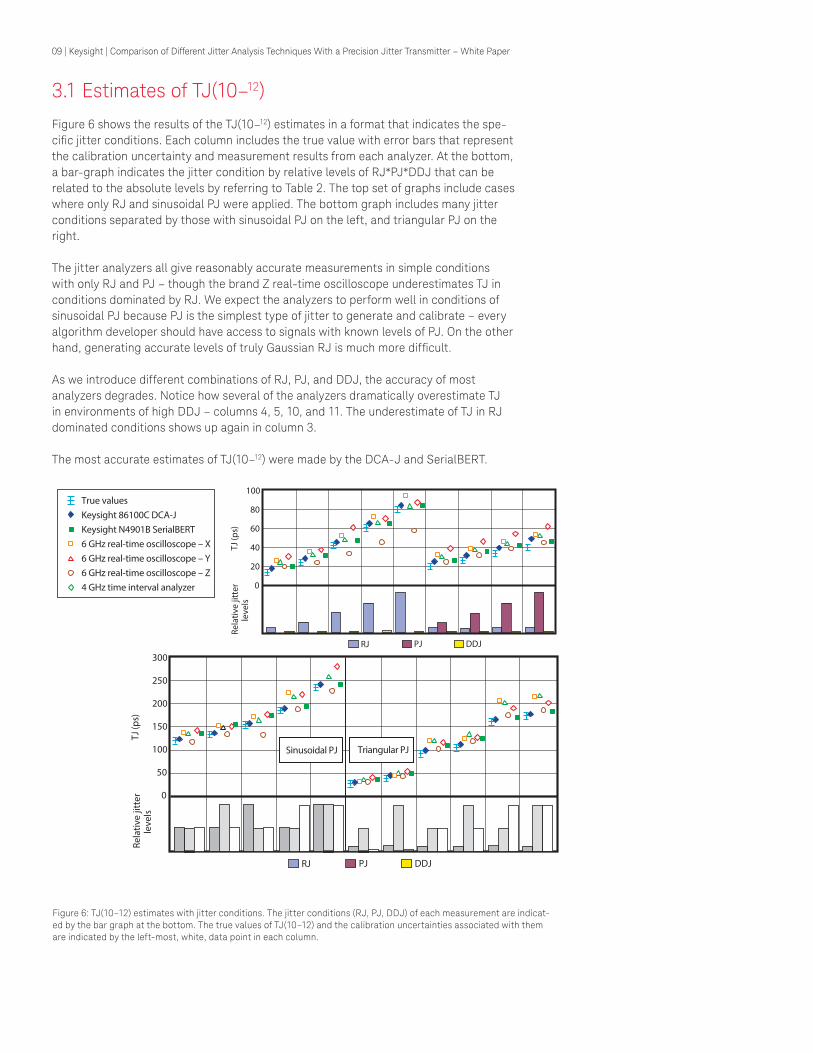
Figure 6 shows the results of the TJ(10–12) estimates in a format that indicates the spe-cific jitter conditions. Each column includes the true value with error bars that represent the calibration uncertainty and measurement results from each analyzer. At the bottom, a bar-graph indicates the jitter condition by relative levels of RJ*PJ*DDJ that can be related to the absolute levels by referring to Table 2. The top set of graphs include cases where only RJ and sinusoidal PJ were applied. The bottom graph includes many jitter conditions separated by those with sinusoidal PJ on the left, and triangular PJ on the right.

The jitter analyzers all give reasonably accurate measurements in simple conditions with only RJ and PJ – though the brand Z real-time oscilloscope underestimates TJ in conditions dominated by RJ. We expect the analyzers to perform well in conditions of sinusoidal PJ because PJ is the simplest type of jitter to generate and calibrate – every algorithm developer should have access to signals with known levels of PJ. On the other hand, generating accurate levels of truly Gaussian RJ is much more difficult.

As we introduce different combinations of RJ, PJ, and DDJ, the accuracy of most analyzers degrades. Notice how several of the analyzers dramatically overestimate TJ in environments of high DDJ – columns 4, 5, 10, and 11. The underestimate of TJ in RJ dominated conditions shows up again in column 3.

The most accurate estimates of TJ(10–12) were made by the DCA-J and SerialBERT.

Figure 6: TJ(10–12) estimates with jitter conditions. The jitter conditions (RJ, PJ, DDJ) of each measurement are indicat-ed by the bar graph at the bottom. The true values of TJ(10–12) and the calibration uncertainties associated with them are indicated by the left-most, white, data point in each column.


PJRJ DDJ

300

250

200

150

100

50

0

Rela

tive

jitte

rle

vels

TJ (p

s)

Sinusoidal PJ Triangular PJ

PJRJ DDJ

100

80

60

40

20

0

Rela

tive

jitte

rle

vels

TJ (p

s)


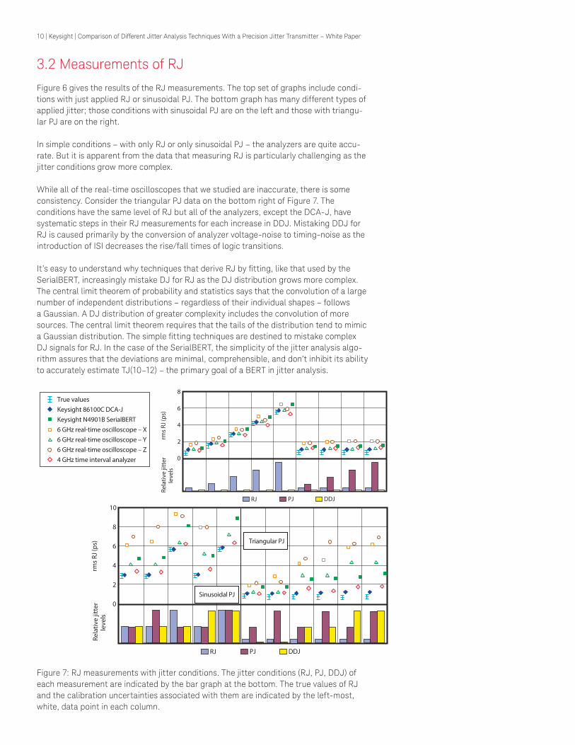
3.2 Measurements of RJ

Figure 6 gives the results of the RJ measurements. The top set of graphs include condi-tions with just applied RJ or sinusoidal PJ. The bottom graph has many different types of applied jitter; those conditions with sinusoidal PJ are on the left and those with triangu-lar PJ are on the right.

In simple conditions – with only RJ or only sinusoidal PJ – the analyzers are quite accu-rate. But it is apparent from the data that measuring RJ is particularly challenging as the jitter conditions grow more complex.

While all of the real-time oscilloscopes that we studied are inaccurate, there is some consistency. Consider the triangular PJ data on the bottom right of Figure 7. The conditions have the same level of RJ but all of the analyzers, except the DCA-J, have systematic steps in their RJ measurements for each increase in DDJ. Mistaking DDJ for RJ is caused primarily by the conversion of analyzer voltage-noise to timing-noise as the introduction of ISI decreases the rise/fall times of logic transitions.

It’s easy to understand why techniques that derive RJ by fitting, like that used by the SerialBERT, increasingly mistake DJ for RJ as the DJ distribution grows more complex. The central limit theorem of probability and statistics says that the convolution of a large number of independent distributions – regardless of their individual shapes – follows a Gaussian. A DJ distribution of greater complexity includes the convolution of more sources. The central limit theorem requires that the tails of the distribution tend to mimic a Gaussian distribution. The simple fitting techniques are destined to mistake complex DJ signals for RJ. In the case of the SerialBERT, the simplicity of the jitter analysis algo-rithm assures that the deviations are minimal, comprehensible, and don’t inhibit its ability to accurately estimate TJ(10–12) – the primary goal of a BERT in jitter analysis.

Figure 7: RJ measurements with jitter conditions. The jitter conditions (RJ, PJ, DDJ) of each measurement are indicated by the bar graph at the bottom. The true values of RJ and the calibration uncertainties associated with them are indicated by the left-most, white, data point in each column.


PJRJ DDJ

10

8

6

4

2

0

Rela

tive

jitte

rle

vels

rms

RJ (p

s)

Sinusoidal PJ

Triangular PJ

PJRJ DDJ

8

6

4

2

0

Rela

tive

jitte

rle

vels

rms

RJ (p

s)


Only the DCA-J performs accurate RJ measurements within the calibration accuracy for all test conditions. One of the other analyzers, the TIA, indicated by the hollow red diamonds symbol, is consistent in most cases. The technique for measuring RJ used by these two analyzers is similar in one respect: they both separate correlated and uncor-related jitter prior to measuring RJ.

3.3 Measurements of DJExactly what is reported as DJ by some of the analyzers is not obvious. As explained in Ref. [4] the important observable is the dual-Dirac value of DJ, not the actual peak-to-peak value. The DCA-J and SerialBERT report the dual-Dirac value for DJ. Since most of the jitter conditions we studied had a small RJ:DJ ratio, the difference between peak-to-peak DJ and dual-Dirac DJ is small – less than 5 ps – within the systematic uncer-tainty of the calibration. We assume that the other analyzers also report the dual Dirac DJ. Regardless of what we assume, the key point remains that the measurements are inconsistent.

The uncertainties in the dual-Dirac DJ are larger than you might expect from the un-certainties of the individual source DJ values in Table 2. Unlike for the peak-to-peak DJ, because of its model dependence, the RJ uncertainty propagates into the dual-Dirac DJ.

Figure 8: Measurements of the dual-Dirac DJ with jitter conditions. The jitter conditions (RJ, PJ, DDJ) of each measurement are indicated by the bar graph at the bottom. The true values of dual-Dirac DJ and the calibration uncertainties associated with them are indicated by the left-most, white, data point in each column.


PJRJ DDJ

200

150

100

50

0

Rela

tive

jitte

rle

vels

dua

l-Dira

c D

J (ps

)

Sinusoidal PJ

Triangular PJ

PJRJ DDJ

50

40

30

20

10

0

Rela

tive

jitte

rle

vels

dual

-Dira

c D

J (ps

)


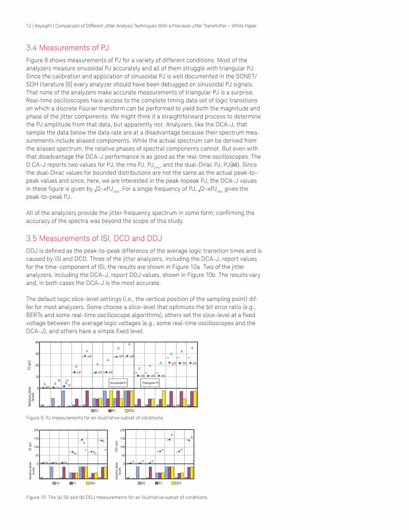
3.4 Measurements of PJFigure 9 shows measurements of PJ for a variety of different conditions. Most of the analyzers measure sinusoidal PJ accurately and all of them struggle with triangular PJ. Since the calibration and application of sinusoidal PJ is well documented in the SONET/SDH literature [6] every analyzer should have been debugged on sinusoidal PJ signals. That none of the analyzers make accurate measurements of triangular PJ is a surprise. Real-time oscilloscopes have access to the complete timing data set of logic transitions on which a discrete Fourier transform can be performed to yield both the magnitude and phase of the jitter components. We might think it a straightforward process to determine the PJ amplitude from that data, but apparently not. Analyzers, like the DCA-J, that sample the data below the data rate are at a disadvantage because their spectrum mea-surements include aliased components. While the actual spectrum can be derived from the aliased spectrum, the relative phases of spectral components cannot. But even with that disadvantage the DCA-J performance is as good as the real-time oscilloscopes. The D CA-J reports two values for PJ, the rms PJ, PJrms, and the dual-Dirac PJ, PJ(δδ). Since the dual-Dirac values for bounded distributions are not the same as the actual peak-to-peak values and since, here, we are interested in the peak-topeak PJ, the DCA-J values in these figure is given by √2–xPJrms. For a single frequency of PJ, √2–xPJrms gives the peak-to-peak PJ.

All of the analyzers provide the jitter-frequency spectrum in some form; confirming the accuracy of the spectra was beyond the scope of this study.

3.5 Measurements of ISI, DCD and DDJDDJ is defined as the peak-to-peak difference of the average logic transition times and is caused by ISI and DCD. Three of the jitter analyzers, including the DCA-J, report values for the time-component of ISI, the results are shown in Figure 10a. Two of the jitter analyzers, including the DCA-J, report DDJ values, shown in Figure 10b. The results vary and, in both cases the DCA-J is the most accurate.

The default logic slice-level settings (i.e., the vertical position of the sampling point) dif-fer for most analyzers. Some choose a slice-level that optimizes the bit error ratio (e.g., BERTs and some real-time oscilloscope algorithms), others set the slice-level at a fixed voltage between the average logic voltages (e.g., some real-time oscilloscopes and the DCA-J), and others have a simple fixed level.

PJRJ DDJ

40

30

20

10

0

Rela

tive

jitte

rle

vels

PJ (

ps)

Sinusoidal PJ Triangular PJ

Figure 10: The (a) ISI and (b) DDJ measurements for an illustrative subset of conditions.

PJRJ DDJ

200

150

100

50

0

Rela

tive

jitte

rle

vels

ISI (

ps)

PJRJ DDJ

200

150

100

50

0

Rela

tive

jitte

rle

vels

DD

J (ps

)

Figure 9: PJ measurements for an illustrative subset of conditions.

Figure 10: The (a) ISI and (b) DDJ measurements for an illustrative subset of conditions.


4. Why Some Test Sets Get It Right And Some Get It Wrong

The DCA-J is the most accurate jitter analysis tool available. The DCA-J does not con-fuse DDJ for RJ; it has a very low voltage noise floor and an algorithm that uses a spec-tral technique for measuring RJ after the jitter data has been separated into correlated (DDJ) and uncorrelated (RJ*PJ) subsets. No other analyzer combines the quietest hard-ware and the key combination of algorithms in the right order.

The SerialBERT is the only analyzer on which estimates of TJ(BER) can be verified by actual measurements – hardly an irrelevant feature. The simplicity of the BERT tech-nique makes it easy to understand under what conditions its fast TJ(BER) estimate might overestimate the truth and encourage the savvy engineer to appropriately tune the BER threshold and the number of transmitted bits per time-delay appropriately.

4.1 Use high quality acquisition hardwareThe precision of any measurement system is limited by its hardware performance. The best algorithm applied to poor hardware won’t provide accurate results [8].

4.1.1 Voltage noiseThe voltage noise floor of the acquisition hardware affects the jitter analysis results by corrupting the time measurement of logic transitions. Consider the extremes, for very fast rise/fall times – vertical edges – fluctuations in the signal voltage don’t affect the timing of logic transitions; but as the rise/fall times slow, flattening out edges, voltage fluctuations can change the timing. Thus, the effect of an analyzer’s voltage noise on it’s RJ accuracy depends on the rise/fall time of the signal. Generally, an analyzer’s voltage noise to timing noise conversion is related to the product of the analyzer’s voltage noise and the signal’s rise/fall time. The voltage noise, independent of the vertical component of ISI, is primarily random and so affects RJ measurements.

The precision jitter transmitter generated ISI through the filtering and attenuation effects of a backplane. In addition to increased DDJ from the time-component of ISI, the vertical component of ISI slows the rise/fall times. Ignoring algorithmic effects, Figure 7 shows how the RJ measurement results increase with slower rise/fall times for those analyzers with appreciable voltage noise.

The voltage noise floor of real-time oscilloscopes is roughly proportional to the setting of their vertical sensitivity down to a minimum absolute noise floor. For the real-time oscilloscopes in this study the noise floors were approximately 30 to 40 mdiv rms. With vertical sensitivity set to 100 mV/div they had effective voltage noise floors of 3 to 4 mV rms. The voltage noise floor of the DCA-J is typically 0.25 mV.

Jitter analysis on a BERT is affected by the minimum voltage difference that the error detector can discriminate – the error detector sensitivity. For example, the error detec-tor sensitivity of the SerialBERT is less than 50 mV. In the worst case, 50 mV sensitivity means that logic levels cannot be distinguished if they are separated by less than 50 mV. The error detector sensitivity determines the minimum observable TJ that a BERT can measure and causes a small bias in TJ measurements that is proportional to the signal’s rise/fall time.

4.1.2 Sampling clock jitterThe sampling clock jitter of real-time oscilloscopes is comprised of both RJ and DJ. The RJ component of the sampling clock jitter depends on the clock reference used for the measurement. Fixed frequency imbedded-clock reference measurements can be


susceptible to the oscilloscope’s time-base close-to-carrier phase noise, if the real-time waveform acquisitions become too long – which was not an issue for the acquisition times used in this study. Software phase-locked-loop clock and explicit clock reference measurements are not affected by the time-base close-to-carrier phase noise. The re-al-time oscilloscopes studied in this paper had sample clock RJ of, σ ~ 0.7 to 1.2 ps. The DJ is dominated by multiple PJ components whose amplitudes ranged from 0.1 to 1 ps.

The sampling clock jitter of a good BERT is typically < 0.5 ps.

Sampling clock jitter is not relevant to jitter analysis on sampling oscilloscopes (e.g., the DCA-J) or TIAs.

4.1.3 Trigger jitterTrigger jitter is dominated by RJ and sets the lower limit on the observable RJ of an ana-lyzer. The trigger jitter of the DCA-J is typically 0.8 ps or, if the DCA-J is equipped with a precision time-base (Keysight 86107A), less than 0.2 ps.

Trigger jitter does not affect jitter analysis techniques used by the real-time oscillo-scopes that we studied and the analogous term for BERTs is sampling jitter, discussed below.

4.1.4 Time-base linearityThe measurement error of logic transition timing is limited by the linearity of the analyzer’s time-base. The time-base nonlinearity of real-time oscilloscopes is very small and does note affect the jitter measurement algorithms. By using a hardware pattern-locked trigger, the DCA-J time-base nonlinearity relevant to jitter analysis is negligible. The nonlinearity of BERT time-bases varies a great deal from model to model, typically 1/2 to 2 ps.

4.1.5 Transition time accuracyThe test equipment that we studied use three different techniques for determining the time of a logic transition. The input signal to the real-time oscilloscopes were digitized at 20 GSa/s giving several data points for each bit. The time position at the voltage slice level, the transition time, is determined by interpolating between the two samples on either side of the slice level. The timing accuracy is limited by the interpolation uncertainty and the linearity of the analog to digital conversion – which is usually excellent.

TIAs use a linear voltage ramp from the time of a trigger signal to the time of a logic tran-sition to determine transition times. The timing transition is limited by the intrinsic jitter of the trigger, the voltage ramp latch, and voltage ramp linearity.

The DCA-J technique derives sixteen different edge models for the voltage to time transfer function. Conceptually, the technique is not unlike interpolation; a set of data from a given edge in the test pattern is used to determine the behavior of that edge so that the transi-tion time information for every bit sampled can be derived. The only drawback to the edge model technique s that it limits the maximum level of jitter that the DCA-J can analyze. The maximum decipherable jitter amplitude is decreases for faster rise/fall times. For details see Ref. [5].

The BERT technique is truly digital. Each bit in the signal is analyzed to determine wheth-er or not the logic level at the time-delay setting of the BERT error detector was above or below the slice level. The bit is then identified as a ‘1’ or a ‘0’ and compared to the known test pattern to determine whether or not the identification is an error. The uncertainty in that determination is limited by the error detector sensitivity and sampling clock jitter.


4.1.6 BandwidthBandwidth has two opposing effects. First, the bandwidth of the analyzer must be large enough to accurately portray the signal. Low bandwidths filter low harmonics, increasing the rise/fall time of the signal. The increased rise/fall time in turn exacerbates the problem of the analyzer’s voltage noise. Low analyzer bandwidths can also introduce ISI that can cause inaccurate ISI, DDJ, DCD, and DJ measurements. Second, the bandwidth of the analyzer should be low enough to limit the out-of-band voltage noise of the signal. The real-time oscilloscopes all had 6 GHz bandwidths, the TIA, 4 GHz, and the DCA-J 20 GHz.

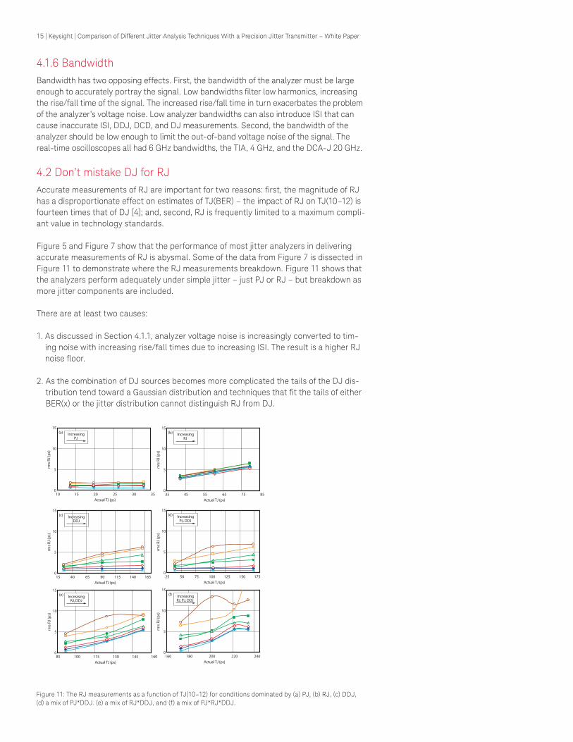
4.2 Don’t mistake DJ for RJAccurate measurements of RJ are important for two reasons: first, the magnitude of RJ has a disproportionate effect on estimates of TJ(BER) – the impact of RJ on TJ(10–12) is fourteen times that of DJ [4]; and, second, RJ is frequently limited to a maximum compli-ant value in technology standards.

Figure 5 and Figure 7 show that the performance of most jitter analyzers in delivering accurate measurements of RJ is abysmal. Some of the data from Figure 7 is dissected in Figure 11 to demonstrate where the RJ measurements breakdown. Figure 11 shows that the analyzers perform adequately under simple jitter – just PJ or RJ – but breakdown as more jitter components are included.

There are at least two causes:

1. As discussed in Section 4.1.1, analyzer voltage noise is increasingly converted to tim-ing noise with increasing rise/fall times due to increasing ISI. The result is a higher RJ noise floor.

2. As the combination of DJ sources becomes more complicated the tails of the DJ dis-tribution tend toward a Gaussian distribution and techniques that fit the tails of either BER(x) or the jitter distribution cannot distinguish RJ from DJ.

Figure 11: The RJ measurements as a function of TJ(10–12) for conditions dominated by (a) PJ, (b) RJ, (c) DDJ, (d) a mix of PJ*DDJ. (e) a mix of RJ*DDJ, and (f) a mix of PJ*RJ*DDJ.

Figure 11: The RJ measurements as a function of TJ(10–12) for conditions dominated by (a) PJ, (b) RJ, (c) DDJ, (d) a mix of PJ *DDJ. (e) a mix of RJ *DDJ, and (f) a mix of PJ *RJ *DDJ.

15

10

5

0

rms

RJ (p

s)

10 15 20 25 30 35

Increasing PJ

(a)

Actual TJ (ps)

15

10

5

0

rms

RJ (p

s)

35 45 55 65 75 85

Increasing RJ

(b)

Actual TJ (ps)

15

10

5

0

rms

RJ (p

s)

25 50 75 100 125 150 175

Increasing PJ, DDJ

(d)

Actual TJ (ps)

15

10

5

0

rms

RJ (p

s)

15 40 65 90 115 140 165

Increasing DDJ

(c)

Actual TJ (ps)

15

10

5

0

rms

RJ (p

s)

160 180 200 220 240

Increasing RJ, PJ, DDJ

(f)

Actual TJ (ps)

15

10

5

0

rms

RJ (p

s)

85 100 115 130 145 160

Increasing RJ, DDJ

(e)

Actual TJ (ps)


4.2.1 Separate correlated and uncorrelated jitter firstAs DDJ is introduced the quality of most RJ measurements degrades rapidly. To avoid confusing DDJ for RJ it is necessary to separate correlated and uncorrelated jitter and then extract RJ from the uncorrelated jitter data. The two techniques with the most ac-curate RJ measurements, the DCA-J and the TIA, indicated by the hollow red diamonds use knowledge of the test pattern to remove DDJ from the RJ analysis. The DCA-J uses a technique based on an automatic pattern trigger to remove DDJ from the distribution [5].

4.2.2 Use an independent spectral technique for measuring RJOnce the DDJ is removed from the distribution, equating RJ to the rms noise in the jitter-frequency spectrum gives the most accurate RJ results. The reason the spectral technique is most accurate is simple. Accurate fits to the tails of BER(x) or the jitter dis-tribution require a statistical sample large enough to assure that the region included in the fit is dominated by RJ, not DJ. While removing the correlated jitter goes a long way, uncorrelated jitter – e.g., triangular PJ – can distort the fit.

4.3 Don’t tweak the algorithm parameters too muchThat the brand Z real-time oscilloscope, indicated by the hollow brown circles, underesti-mates TJ in RJ dominated environments provides an interesting example. It measures RJ and DJ with reasonable accuracy under RJ dominated conditions – Figure 7 and Figure 8 – but doesn’t translate that success into accurate estimates of TJ(10–12), Figure 6. The analyzer uses a fitting technique to measure RJ and DJ similar in principle to the stan-dard dual-Dirac fitting algorithm performed by a BERT. That the RJ/DJ accuracy doesn’t translate to TJ(10–12) accuracy indicates that the algorithmic parameters have been tuned improperly. Since truly Gaussian RJ is difficult to generate in the lab, it is easy to speculate that an algorithm may have been tuned under non-Gaussian circumstances.

5. The Jitter Analysis Techniques Introduced On The DCA-J Solve The Problem. Finally.Engineers have known for years that different jitter analyzers give conflicting results. By using a precision jitter transmitter we were able to make quantitative statements about the accuracy of each analyzer under a wide variety of jitter conditions. The jitter conditions created by the transmitter were carefully designed for consistence with the standard industry assumptions that RJ follows an unbounded Gaussian distribution and that the DJ distribution is bounded. While it is reasonable to debate the veracity of the assumptions, the analysis techniques used by all jitter analyzers of the type studied here rest on these assumptions. A fair comparison of the different techniques therefore requires that the assumptions are met in the test environment. The test conditions werechosen to represent common situations faced by design engineers – jitter levels at or near the standard budgets.

While our understanding of the techniques used on the non-Keysight equipment was not complete, we were able to identify the key elements of a jitter analyzer that are nec-essary for making accurate estimates of TJ(BER) and measurements of RJ, DJ, PJ, and DDJ.

The challenging hardware element for a jitter analyzer is a low voltage noise floor. Equip-ment specifications related to timing, trigger jitter, sampling jitter, time-base linearity, and transition time accuracy on the jitter analyzers were all up to the task. It was the conver-sion of analyzer amplitude noise to timing noise that caused the biggest inaccuracies.


While the analysis algorithms are always limited by the acquisition hardware, we found two keys to accurate jitter analysis techniques. First, DDJ should be removed from the data prior to measuring RJ; and second, a spectral technique should be used where the rms continuum noise is identified as RJ.

Crosstalk was included in Figure 1 because it is often assumed to be jitter. Crosstalk is an example of bounded uncorrelated jitter (BUJ). We did not include a crosstalk signal in the precision jitter transmitter because none of the jitter analyzers claims to be capable of measuring it and there is no typical crosstalk signal. Crosstalk is amplitude noise. Consider the case of a data channel running parallel to a channel under test. If the fre-quencies of the two signals are locked, then there is a fixed phase offset between them. If that phase is 90 degrees, then the eye of the signal under test will have a depression in the center that lowers the BER – obviously amplitude noise. If the two signals are in phase, then the amplitude noise experienced by the signal under test is concentrated at the crossing point and looks like jitter – but it’s not. A way to work around the aggressor problem is to measure RJ with the crosstalk turned off, and then repeat the measure-ment with crosstalk turned on, but σ fixed to the value measured without crosstalk.

5.1 ConclusionThe only way to judge which technique is best is with a precision jitter transmitter where the answers are known before the measurements are made. We built the precision jitter transmitter to determine the best method for jitter analysis; to determine the combi-nation of techniques that not only gives consistently accurate estimates for total jitter defined at a bit error ratio, but also gives accurate measurements of the jitter subcom-ponents. By subjecting the market leading jitter analyzers to known jitter conditions we have shown that Keysight 86100C DCA-J is the most accurate jitter analyzer available. The methods used by the DCA-J are fully described in Ref. [5] and by the SerialBERT in Ref. [6] – the techniques of the other analyzers are not fully documented and it is ap-parent that none of them have been confirmed against a well-calibrated precision jitter transmitter.

Having formulated the most accurate jitter analysis technique on our equivalent-time sampling oscilloscope, the DCA-J, we are implementing the important components of our techniques in our real-time oscilloscope jitter analysis tool, EZJIT+. Once EZJIT+ has been challenged by the precision jitter transmitter we will publish its performance in a separate whitepaper.


References

1 Jim Stimple and Ransom Stephens, “Precision Jitter Transmitter,” DesignCon 2005, http://www.designcon.com/conference/7-wa1.html.

2 To learn about the basics of jitter analysis, see Ransom Stephens, “The rules of jitter analysis,” http://www.analogzone.com/nett0927.pdf, 2004; and Ransom Stephens, “Analyzing Jitter at High Data Rates,” IEEE Communications Magazine, vol. 42, no. 2, February 2004, pp. 6-10.

3 Keysight Technologies’ Application Note, “Jitter Fundamentals: Keysight 81250 Par-BERT Jitter Injection and Analysis Capabilities,” Literature Number AN-5988-9756EN, available from www.Keysight.com, 2003.

4 Ransom Stephens, “Jitter analysis: The dual-Dirac model, RJ/DJ, and Q-scale,” Key-sight Technologies Whitepaper, 2004. Available from www.Keysight.com.

5 Keysight Technologies Product Note, 86100C-1, “Precision jitter analysis using the Keysight 86100C DCA-J,” Keysight Literature Number 5989-1146EN, http://cp.literature.keysight.com/litweb/pdf/5989-1146EN.pdf.

6 Keysight Tutorial, “Understanding Jitter and Wander Measurements and Standards, Second Edition,” Keysight Literature number 5988-6254EN, 2003. Available from www.Keysight.com.

7 Marcus Müller, Ransom Stephens, and Russ McHugh, “Total Jitter Measurement at Low Probability Levels, Using Optimized BERT Scan Method,” DesignCon 2005, http://www.designcon.com/conference/7-ta4.html.

8 Steve Draving, “How Accurate Are Your Jitter Measurements,” DesignCon 2003.

http://www.designcon.com/conference/7-wa1.html

http://www.analogzone.com/nett0927.pdf

http://cp.literature.keysight.com/litweb/pdf/5989-1146EN.pdf

http://www.designcon.com/conference/7-ta4.html


This information is subject to change without notice.© Keysight Technologies, 2017Published in USA, December 1, 20175989-3205ENwww.keysight.com

www.keysight.com/find/dca

For more information on Keysight Technologies’ products, applications or services, please contact your local Keysight office. The complete list is available at:www.keysight.com/find/contactus

Americas Canada (877) 894 4414Brazil 55 11 3351 7010Mexico 001 800 254 2440United States (800) 829 4444

Asia PacificAustralia 1 800 629 485China 800 810 0189Hong Kong 800 938 693India 1 800 11 2626Japan 0120 (421) 345Korea 080 769 0800Malaysia 1 800 888 848Singapore 1 800 375 8100Taiwan 0800 047 866Other AP Countries (65) 6375 8100

Europe & Middle EastAustria 0800 001122Belgium 0800 58580Finland 0800 523252France 0805 980333Germany 0800 6270999Ireland 1800 832700Israel 1 809 343051Italy 800 599100Luxembourg +32 800 58580Netherlands 0800 0233200Russia 8800 5009286Spain 800 000154Sweden 0200 882255Switzerland 0800 805353

Opt. 1 (DE)Opt. 2 (FR)Opt. 3 (IT)

United Kingdom 0800 0260637

For other unlisted countries:www.keysight.com/find/contactus(BP-9-7-17)

DEKRA CertifiedISO9001 Quality Management System

www.keysight.com/go/qualityKeysight Technologies, Inc.DEKRA Certified ISO 9001:2015Quality Management System

Evolving Since 1939Our unique combination of hardware, software, services, and people can help you reach your next breakthrough. We are unlocking the future of technology. From Hewlett-Packard to Agilent to Keysight.

myKeysightwww.keysight.com/find/mykeysightA personalized view into the information most relevant to you.

http://www.keysight.com/find/emt_product_registrationRegister your products to get up-to-date product information and find warranty information.

Keysight Serviceswww.keysight.com/find/serviceKeysight Services can help from acquisition to renewal across your instrument’s lifecycle. Our comprehensive service offerings—one-stop calibration, repair, asset management, technology refresh, consulting, training and more—helps you improve product quality and lower costs.

Keysight Assurance Planswww.keysight.com/find/AssurancePlansUp to ten years of protection and no budgetary surprises to ensure your instruments are operating to specification, so you can rely on accurate measurements.

Keysight Channel Partnerswww.keysight.com/find/channelpartnersGet the best of both worlds: Keysight’s measurement expertise and product breadth, combined with channel partner convenience.

http://www.keysight.com

http://www.keysight.com/find/dca

http://www.keysight.com/find/contactus

http://www.keysight.com/find/contactus

http://www.keysight.com/go/quality

http://www.keysight.com/find/mykeysight

http://www.keysight.com/find/emt_product_registration

http://www.keysight.com/find/service

http://www.keysight.com/find/AssurancePlans

http://www.keysight.com/find/channelpartners

keysight technologies comparison of different jitter analysis...

Documents