Keynesian Economics, Monetary Policy and the Business

Cycle - New and Old

Alex Cukierman∗

September 12 2005

Abstract

After a brief review of the main differences between New and Old Keynesian economics

from the sixties this paper focusses on a tension between traditional sluggish measures of

potential output commonly used by policymakers and the New Keynesian (NK) notion of

this variable which conceptualizes it as the level of output that would have been produced

under perfect competition had all prices and wages been flexible. The paper shows that,

under monopolistic competition, NK potential output is often more volatile than the level

of output produced under sticky prices and wages implying either of the following. Real life

policymakers mistakenly target smooth versions of output or (since actual economies are

monopolistically rather than perfectly competitive) the flexible price and wage equilibrium

does not necessarily maximize welfare. The paper shows, that depending on the shape of

the utility function and of the distribution of productivity shocks either case is possible

and proposes a criterion for discriminating between them.

JEL Classification: E3, E4, E5, E6

∗Berglas School of Economics, Tel-Aviv University and CEPR. I would like to thank two anonymous referees,Jordi Gali, Marvin Goodfriend, Assaf Razin, Yona Rubunstein, Frank Smets and Michael Woodford for usefulreactions. Ehud Menirav and Oren Shapir provided excellent research support. The usual disclaimer applies.Earlier versions were presented as a keynote lecture at the July 2004 CES-ifo Venice workshop on ”AggregateDemand Management Policies: Back to Keynes?”, at Tel-Aviv University and at Haifa University.

1

1 Introduction

Macroeconomics has undergone substantial methodological developments and swings since the

heydays of Keynesianism in the sixties. At that time the view that output is largely demand

determined and that the price level can be taken, to a first approximation, as fixed was widely

accepted by both academics and policymakers. The great inflation of the seventies revived the

classical-monetarist view that output is determined mainly by productive capacity, that prices

are flexible, and that changes in demand and in monetary stance mainly affect the price level, at

least after a while. This was followed by the emergence of real business cycle models. Starting

from preferences, technology, individual dynamic optimization under perfect competition and

the premise that prices are flexible this body of research attributed business cycle fluctuations

mainly to technology shocks, changes in preferences, taxation and other real reasons. During

the last decade, temporarily sticky prices have been resuscitated by incorporating them, along

with monopolistic competition into real business cycle models. This opened the door for a more

explicit treatment of monetary policy within real business cycle models and produced the recent

body of research known as New Keynesian economics.1

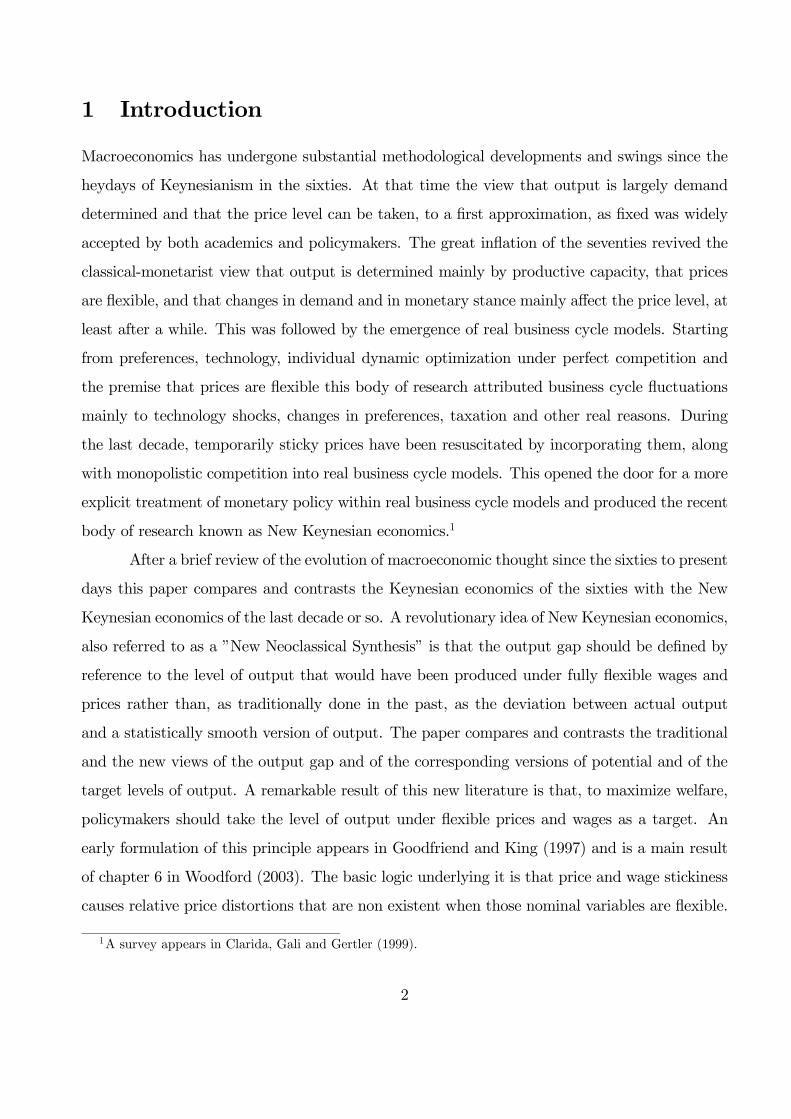
After a brief review of the evolution of macroeconomic thought since the sixties to present

days this paper compares and contrasts the Keynesian economics of the sixties with the New

Keynesian economics of the last decade or so. A revolutionary idea of New Keynesian economics,

also referred to as a ”New Neoclassical Synthesis” is that the output gap should be defined by

reference to the level of output that would have been produced under fully flexible wages and

prices rather than, as traditionally done in the past, as the deviation between actual output

and a statistically smooth version of output. The paper compares and contrasts the traditional

and the new views of the output gap and of the corresponding versions of potential and of the

target levels of output. A remarkable result of this new literature is that, to maximize welfare,

policymakers should take the level of output under flexible prices and wages as a target. An

early formulation of this principle appears in Goodfriend and King (1997) and is a main result

of chapter 6 in Woodford (2003). The basic logic underlying it is that price and wage stickiness

causes relative price distortions that are non existent when those nominal variables are flexible.

1A survey appears in Clarida, Gali and Gertler (1999).

2

Hence, a monetary policy aimed at replicating the flexible price and wage allocation, in the

presence of stickiness in those nominal variables, eliminates those distortions.

A main result of this paper is that, under reasonable circumstances, this output level

may be more volatile than the level of output under sticky prices and wages implying that

policymakers suscribing to this New Keynesian policy recommendation would have to allow

output to fluctuate more than under sticky prices and wages. This result is obtained within a

microfounded illustrative framework by comparing the equilibria obtained in the case in which

prices and nominal wages are fully flexible with the case in which they are sticky. It is a

reality judgement of this author that, even if they had been able to get a measure of output

under flexible prices and wages, most central bankers are currently unlikely to embrace wider

fluctuations in output in order to attain the (more volatile) level of output under flexible prices

and wages. As a matter of fact practically all existing empirical measures of potential output,

starting with those produced by Burns and Mitchell for the US, are designed, at least implicitly,

towards the smoothing of output rather than towards increasing its volatility.

Acceptance of this premise raises an important policy relevant question about the source

of the discrepency between the New Keynesian policy recommendation and actual policy prac-

tice. One possibility is that existing policy procedures are badly structured and should be

revised. Another possibility is that New Keynesian models abstract from some factors that

policymakers rightly pay attention to. For example, the flexible price and wage equilibrium

may not be a first best to start with, due to reasons beyond those caused by sticky prices and

wages. In such a case the general principle of the second best may imply that the addition of a

distortion caused by sticky prices and wages actually improves matters.2

The illustration in the paper allows the flexible price and wage equilibrium to be dis-

torted by recognizing that there is a monopolistic competition distortion that is not offset by

appropriate taxes and subsidies.3 A main result is that, frequently, output and consumption

are less volatile and leisure more volatile when prices and wages are sticky than when they are

2Obviously, those possibilities are not mutually exclusive.3By contrast the early New Keynesian literature often assumes, for simplicity, that any pre-existing steady

state distortion is fully offset by an appropriate system of subsidies cum taxes (Rotemberg and Woodford (1997),Erceg, Henderson and Levin (2000) and chapter 6 of Woodford (2003)). Benigno and Woodford (2004) considerthe more realistic case in which such subsidies are absent.

3

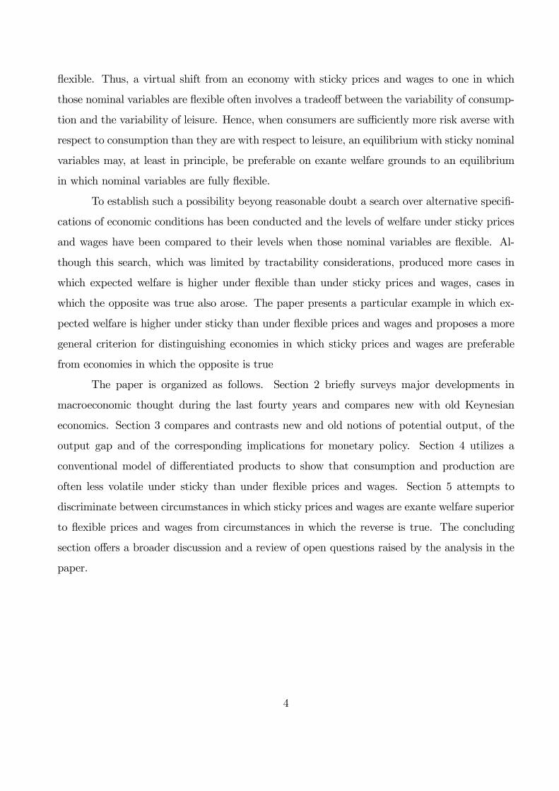
flexible. Thus, a virtual shift from an economy with sticky prices and wages to one in which

those nominal variables are flexible often involves a tradeoff between the variability of consump-

tion and the variability of leisure. Hence, when consumers are sufficiently more risk averse with

respect to consumption than they are with respect to leisure, an equilibrium with sticky nominal

variables may, at least in principle, be preferable on exante welfare grounds to an equilibrium

in which nominal variables are fully flexible.

To establish such a possibility beyong reasonable doubt a search over alternative specifi-

cations of economic conditions has been conducted and the levels of welfare under sticky prices

and wages have been compared to their levels when those nominal variables are flexible. Al-

though this search, which was limited by tractability considerations, produced more cases in

which expected welfare is higher under flexible than under sticky prices and wages, cases in

which the opposite was true also arose. The paper presents a particular example in which ex-

pected welfare is higher under sticky than under flexible prices and wages and proposes a more

general criterion for distinguishing economies in which sticky prices and wages are preferable

from economies in which the opposite is true

The paper is organized as follows. Section 2 briefly surveys major developments in

macroeconomic thought during the last fourty years and compares new with old Keynesian

economics. Section 3 compares and contrasts new and old notions of potential output, of the

output gap and of the corresponding implications for monetary policy. Section 4 utilizes a

conventional model of differentiated products to show that consumption and production are

often less volatile under sticky than under flexible prices and wages. Section 5 attempts to

discriminate between circumstances in which sticky prices and wages are exante welfare superior

to flexible prices and wages from circumstances in which the reverse is true. The concluding

section offers a broader discussion and a review of open questions raised by the analysis in the

paper.

4

2 New Keynesian economics versus the Keynesian con-

sensus of the sixties

I have chosen the sixties as a point of departure against which to compare the recent body of

research dealing with macroeconomic fluctuations and monetary policy known as New Keynesian

Economics (NKE) because the sixties are commonly believed to be the heydays of Keynesianism

in the US. My discussion will be deliberately brief. Fuller accounts of NKE appear in Clarida,

Gali and Gertler (1999), Gali (2003) and Woodford (2003).

2.1 Macroeconomic thought from the sixties to the present - A bird’s

eye view.

As a first pass, a student of macroeconomics during the sixties would have been told that the

behavior of the economy differs depending on whether prices and wages are sticky downward

or whether they are fully flexible. In the first case, if aggregate demand happens to be lower

than productive capacity (or potential output), economic activity is demand determined and

the price level is fixed. In the second, classical case, economic activity is determined by supply

or productive capacity and changes in demand only affect the price level. The appearance of the

Phillips curve (Phillips (1958)) replaced those polar benchmark cases with a, more continuous,

negatively sloped empirical relation between inflation and unemployment. Within a couple of

years this empirical relation was interpreted as reflecting a stable tradeoff between those two

variables The policy implication was that, by being more or less restictive, monetary policy

could position the economy at a point of its choice along this tradeoff (Samuelson and Solow

(1960).

Friedman (1968) disputed this view on the ground that the tradeoff lasts only as long as

inflation is unanticipated. Following the oil shocks of the seventies and Lucas’ (1972, 1973) work

the view that the tradeoff is temporary became widely accepted. This led to a reconsideration

of the relative importance of monetary and of real factors in the generation of business cycles.

Monetary and financial factors were deemphasized and real factors like productivity and taste

shocks were propelled into the center of macroeconomic investigations of the real business cycle

5

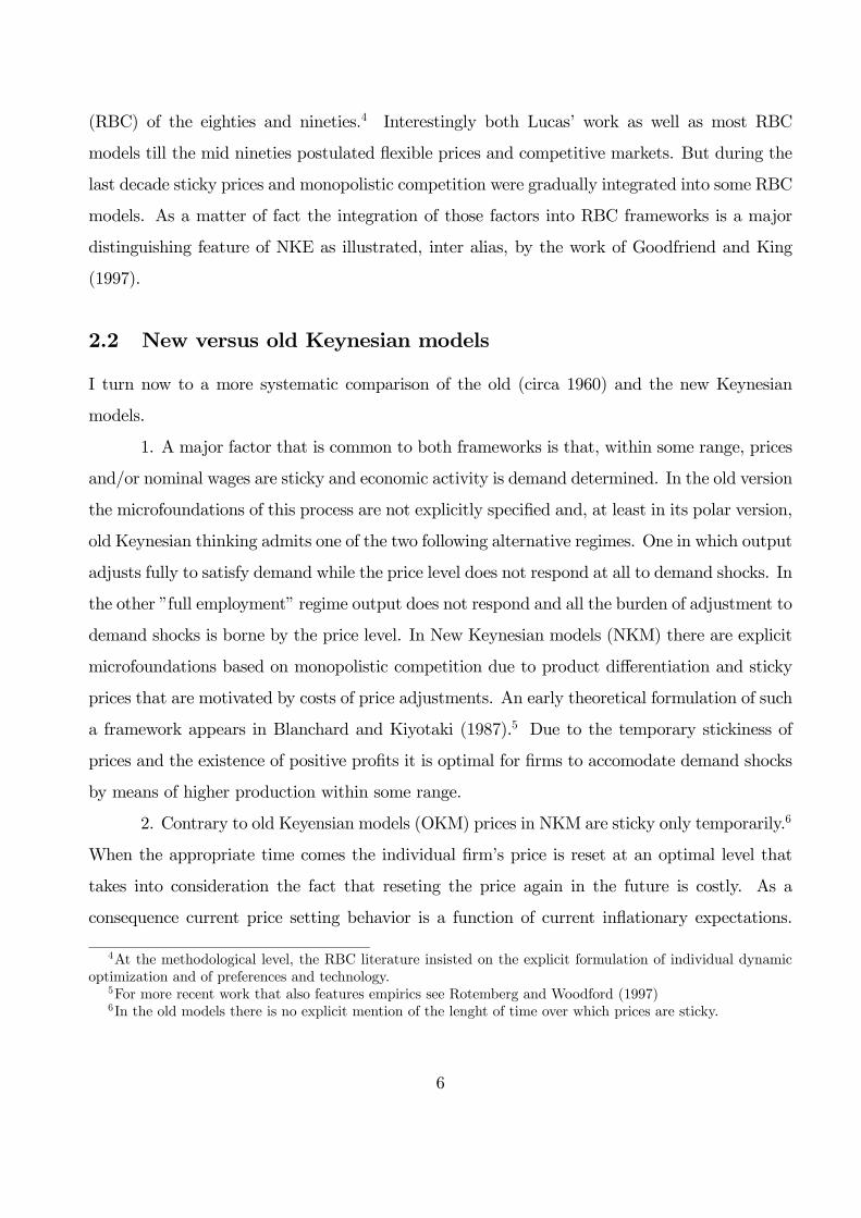
(RBC) of the eighties and nineties.4 Interestingly both Lucas’ work as well as most RBC

models till the mid nineties postulated flexible prices and competitive markets. But during the

last decade sticky prices and monopolistic competition were gradually integrated into some RBC

models. As a matter of fact the integration of those factors into RBC frameworks is a major

distinguishing feature of NKE as illustrated, inter alias, by the work of Goodfriend and King

(1997).

2.2 New versus old Keynesian models

I turn now to a more systematic comparison of the old (circa 1960) and the new Keynesian

models.

1. A major factor that is common to both frameworks is that, within some range, prices

and/or nominal wages are sticky and economic activity is demand determined. In the old version

the microfoundations of this process are not explicitly specified and, at least in its polar version,

old Keynesian thinking admits one of the two following alternative regimes. One in which output

adjusts fully to satisfy demand while the price level does not respond at all to demand shocks. In

the other ”full employment” regime output does not respond and all the burden of adjustment to

demand shocks is borne by the price level. In New Keynesian models (NKM) there are explicit

microfoundations based on monopolistic competition due to product differentiation and sticky

prices that are motivated by costs of price adjustments. An early theoretical formulation of such

a framework appears in Blanchard and Kiyotaki (1987).5 Due to the temporary stickiness of

prices and the existence of positive profits it is optimal for firms to accomodate demand shocks

by means of higher production within some range.

2. Contrary to old Keyensian models (OKM) prices in NKM are sticky only temporarily.6

When the appropriate time comes the individual firm’s price is reset at an optimal level that

takes into consideration the fact that reseting the price again in the future is costly. As a

consequence current price setting behavior is a function of current inflationary expectations.

4At the methodological level, the RBC literature insisted on the explicit formulation of individual dynamicoptimization and of preferences and technology.

5For more recent work that also features empirics see Rotemberg and Woodford (1997)6In the old models there is no explicit mention of the lenght of time over which prices are sticky.

6

This requires the explicit modeling of inflationary expectations which are normally specified

as being model consistent expectations. The optimal reseting of prices and the influence of

inflationary expectations on this activity are absent in the OKM.

3. Asymmetries in upward versus downward adjustments of nominal variables is an

important element of OKM. In particular OKM postulate that prices, and particularly nominal

wages, are more sticky downward than upward.7 By contrast in NKM the degree of nominal

stickiness is independent of the direction of pressure for price change.

4. All firms in the economy normally do not adjust their prices simultaneously. OKM are

silent on this issue. An attractive feature of NKM is that they attempt to evaluate the positive

and normative consequences of price staggering. For tractability reasons the costs of price

adjustment are not modeled explicitly. Folllowing a suggestion by Calvo (1983) it is postulated

instead that each firm can reset its price in any given period with a constant probability that is

smaller than one. As a consequence, when a firm gets the opportunity to reset its price it takes

into consideration that it might not be given such an opportunity again for a number of periods

to come. The firm then sets its price so as to maximize its expected profits. This formalism

is widely used in NKM to evaluate the costs of inflation and to draw conclusions for optimal

monetary policy.8

Sticky prices and wages have also been modeled by assuming that prices and wages in

a given period are preset in the previous period. This alternative modeling approach has been

followed particularly in international macroeconomics. A prominent example is the Obstfeld

and Rogoff (1995) redux paper.

5. Like RBC models on which they are anchored, NKM feature explicit dynamic opti-

mization at the level of the individual economic unit. For the most part OKM of the sixties were

static and did not incorporate micro based consequences of those dynamics like intertemporal

substitution in consumption.

7Recent evidence for the US supports the view that nominal wages are particularly sticky downward (Bewley(1999)).

8Examples appear in Gali (2002), Chapter 3 of Woodford (2003), Schmitt-Grohe and Uribe (2004). Explicitmodeling of the consequences of costs of price adjustments for endogenous price setting decisions have beenextensively studied during the eighties at the micro level. A collection of relevant articles appears in Sheshinskiand Weiss (1993). Endogenous price adjustment decisions have recently been integrated into NKM by Dotseyand King (2005).

7

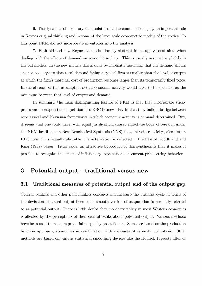
6. The dynamics of inventory accumulations and decummulations play an important role

in Keynes original thinking and in some of the large scale econometric models of the sixties. To

this point NKM did not incorporate inventories into the analysis.

7. Both old and new Keynesian models largely abstract from supply constraints when

dealing with the effects of demand on economic activity. This is usually assumed explicitly in

the old models. In the new models this is done by implicitly assuming that the demand shocks

are not too large so that total demand facing a typical firm is smaller than the level of output

at which the firm’s marginal cost of production becomes larger than its temporarily fixed price.

In the absence of this assumption actual economic activity would have to be specified as the

minimum between that level of output and demand.

In summary, the main distinguishing feature of NKM is that they incorporate sticky

prices and monopolistic competition into RBC frameworks. In that they build a bridge between

neoclassical and Keynsian frameworks in which economic activity is demand determined. But,

it seems that one could have, with equal justification, characterized the body of research under

the NKM heading as a New Neoclassical Synthesis (NNS) that, introduces sticky prices into a

RBC core. This, equally plausible, characterization is reflected in the title of Goodfriend and

King (1997) paper. Titles aside, an attractive byproduct of this synthesis is that it makes it

possible to recognize the effects of inflationary expectations on current price setting behavior.

3 Potential output - traditional versus new

3.1 Traditional measures of potential output and of the output gap

Central bankers and other policymakers conceive and measure the business cycle in terms of

the deviation of actual output from some smooth version of output that is normally referred

to as potential output. There is little doubt that monetary policy in most Western economies

is affected by the perceptions of their central banks about potential output. Various methods

have been used to measure potential output by practitioners. Some are based on the production

function approach, sometimes in combination with measures of capacity utilization. Other

methods are based on various statistical smoothing devices like the Hodrick Prescott filter or

8

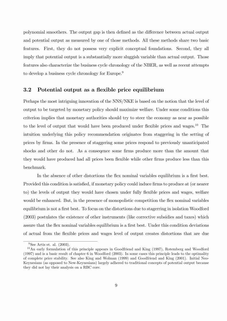
polynomial smoothers. The output gap is then defined as the difference between actual output

and potential output as measured by one of those methods. All these methods share two basic

features. First, they do not possess very explicit conceptual foundations. Second, they all

imply that potential output is a substantially more sluggish variable than actual output. Those

features also characterize the business cycle chronology of the NBER, as well as recent attempts

to develop a business cycle chronology for Europe.9

3.2 Potential output as a flexible price equilibrium

Perhaps the most intriguing innovation of the NNS/NKE is based on the notion that the level of

output to be targeted by monetary policy should maximize welfare. Under some conditions this

criterion implies that monetary authorities should try to steer the economy as near as possible

to the level of output that would have been produced under flexible prices and wages.10 The

intuition underlying this policy recommendation originates from staggering in the setting of

prices by firms. In the presence of staggering some prices respond to previously unanticipated

shocks and other do not. As a conseqence some firms produce more than the amount that

they would have produced had all prices been flexible while other firms produce less than this

benchmark.

In the absence of other distortions the flex nominal variables equilibrium is a first best.

Provided this condition is satisfied, if monetary policy could induce firms to produce at (or nearer

to) the levels of output they would have chosen under fully flexible prices and wages, welfare

would be enhanced. But, in the presence of monopolistic competition the flex nominal variables

equilibrium is not a first best. To focus on the distortions due to stagerring in isolationWoodford

(2003) postulates the existence of other instruments (like corrective subsidies and taxes) which

assure that the flex nominal variables equilibrium is a first best. Under this condition deviations

of actual from the flexible prices and wages level of output creates distortions that are due

9See Artis et. al. (2003).10An early formulation of this principle appears in Goodfriend and King (1997), Rotemberg and Woodford

(1997) and is a basic result of chapter 6 in Woodford (2003). In some cases this principle leads to the optimalityof complete price stability. See also King and Wolman (1999) and Goodfriend and King (2001). Initial Neo-Keynesians (as opposed to New-Keynesians) largely adhered to traditional concepts of potential output becausethey did not lay their analysis on a RBC core.

9

only to staggering. The Calvo formalism makes it possible to characterize those distortions

within a RBC framework and to demonstrate, using quadratic approximations, that welfare is a

decreasing function of the distance between the sticky and the flex nominal variables equilibria.

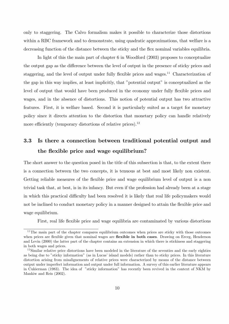
In light of this the main part of chapter 6 in Woodford (2003) proposes to conceptualize

the output gap as the difference between the level of output in the presence of sticky prices and

staggering, and the level of output under fully flexible prices and wages.11 Characterization of

the gap in this way implies, at least implicitly, that ”potential output” is conceptualized as the

level of output that would have been produced in the economy under fully flexible prices and

wages, and in the absence of distortions. This notion of potential output has two attractive

features. First, it is welfare based. Second it is particularly suited as a target for monetary

policy since it directs attention to the distortion that monetary policy can handle relatively

more efficiently (temporary distortions of relative prices).12

3.3 Is there a connection between traditional potential output and

the flexible price and wage equilibrium?

The short answer to the question posed in the title of this subsection is that, to the extent there

is a connection between the two concepts, it is tenuous at best and most likely non existent.

Getting reliable measures of the flexible price and wage equilibrium level of output is a non

trivial task that, at best, is in its infancy. But even if the profession had already been at a stage

in which this practical difficulty had been resolved it is likely that real life policymakers would

not be inclined to conduct monetary policy in a manner designed to attain the flexible price and

wage equilibrium.

First, real life flexible price and wage equilibria are contaminated by various distortions

11The main part of the chapter compares equilibrium outcomes when prices are sticky with those outcomeswhen prices are flexible given that nominal wages are flexible in both cases. Drawing on Erceg, Hendersonand Levin (2000) the latter part of the chapter contains an extension in which there is stickiness and staggeringin both wages and prices.12Similar relative price distortions have been modeled in the literature of the seventies and the early eighties

as being due to ”sticky information” (as in Lucas’ island models) rather than to sticky prices. In this literaturedistortion arising from misalignements of relative prices were characterized by means of the distance betweenoutput under imperfect information and output under full information. A survey of this earlier literature appearsin Cukierman (1983). The idea of ”sticky information” has recently been revived in the context of NKM byMankiw and Reis (2002).

10

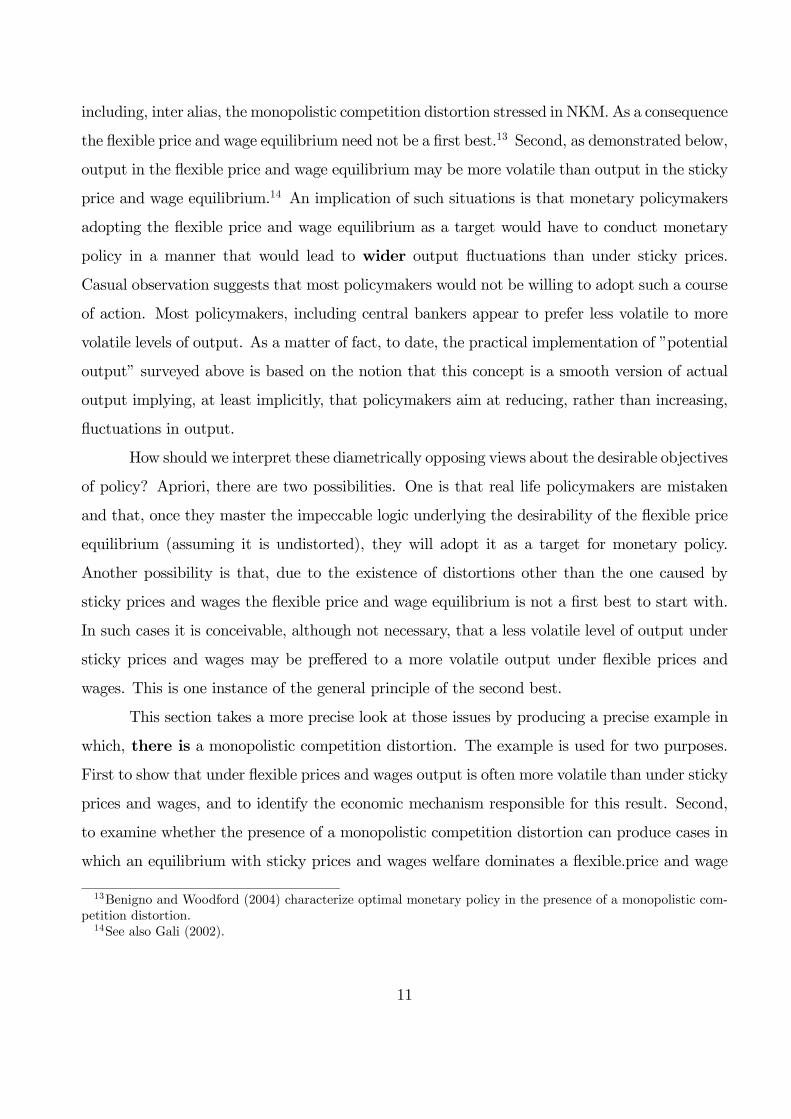
including, inter alias, the monopolistic competition distortion stressed in NKM. As a consequence

the flexible price and wage equilibrium need not be a first best.13 Second, as demonstrated below,

output in the flexible price and wage equilibrium may be more volatile than output in the sticky

price and wage equilibrium.14 An implication of such situations is that monetary policymakers

adopting the flexible price and wage equilibrium as a target would have to conduct monetary

policy in a manner that would lead to wider output fluctuations than under sticky prices.

Casual observation suggests that most policymakers would not be willing to adopt such a course

of action. Most policymakers, including central bankers appear to prefer less volatile to more

volatile levels of output. As a matter of fact, to date, the practical implementation of ”potential

output” surveyed above is based on the notion that this concept is a smooth version of actual

output implying, at least implicitly, that policymakers aim at reducing, rather than increasing,

fluctuations in output.

How should we interpret these diametrically opposing views about the desirable objectives

of policy? Apriori, there are two possibilities. One is that real life policymakers are mistaken

and that, once they master the impeccable logic underlying the desirability of the flexible price

equilibrium (assuming it is undistorted), they will adopt it as a target for monetary policy.

Another possibility is that, due to the existence of distortions other than the one caused by

sticky prices and wages the flexible price and wage equilibrium is not a first best to start with.

In such cases it is conceivable, although not necessary, that a less volatile level of output under

sticky prices and wages may be preffered to a more volatile output under flexible prices and

wages. This is one instance of the general principle of the second best.

This section takes a more precise look at those issues by producing a precise example in

which, there is a monopolistic competition distortion. The example is used for two purposes.

First to show that under flexible prices and wages output is often more volatile than under sticky

prices and wages, and to identify the economic mechanism responsible for this result. Second,

to examine whether the presence of a monopolistic competition distortion can produce cases in

which an equilibrium with sticky prices and wages welfare dominates a flexible.price and wage

13Benigno and Woodford (2004) characterize optimal monetary policy in the presence of a monopolistic com-petition distortion.14See also Gali (2002).

11

equilibrium. The results from those two experiments are then assembled to draw more general

tentative conclusions about the widely established practice of using monetary policy to smooth

output.

4 Flexible prices and wages may lead to more volatile

output than sticky prices and wages - an illustration

The formal example in this section is meant to illustrate that with sticky nominal wages and

prices, output, and therefore income and consumption, are often less volatile when prices and

wages are sticky than when prices and wages are flexible. On the other hand leisure is often

more volatile under sticky than under flexible nominal variables. Those two regimes thus involve

a tradeoff between the volatility of output and consumption on one hand and the volatility

of leisure on the other. This is demonstrated within a framework in which the economy is

hit by transitory productivity shocks, and in which equilibrium employment, production and

consumption fluctuate randomly due to those shocks.

The relatively stabler behavior of production in the sticky price and wage equilibrium

(SPE) is due to the fact that in the flexible price and wage equilibrium (FPE) markups are

constant implying that the real wage goes up and down with transitory productivity shocks.

By contrast in the SPE the real wage is constant creating a, relatively stronger, inverse relation

between employment and productivity than in the FPE. This mitigates the effect of productivity

shocks on the volatility of consumption but raises, in many cases, the volatility of leisure.

The economic mechanism producing those results can be understood roughly by compar-

ing the behavior of firms and of the economy in the face of productivity shocks under flexible

prices and wages with their behavior under sticky prices and wages. In the first case firms adjust

their prices following productivity shocks to maintain their profit maximizing markups in the

face of a nominal wage that adjusts to clear a competitive labor market. As a consequence the

real wage goes up and down with productivity. By contrast, in the sticky nominal variables case

the real wage does not adjust to productivity shocks. In both cases, when productivity goes

down profits go down triggering, a negative pure income effect on leisure which increase the

12

supply of labor and mitigates the decrease in production due to the decrease in productivity.

Under flexible prices there is, additionally, a decrease in the real wage that normally reduces

labor supply. This reduces the mitigating effect of the decrease in profits on the decrease in

output due to the productivity decrease, making output volatilility in the FPE larger than under

the SPE.

4.1 Model

The economy consists of a continuum of individuals on the [0, 1] interval and of a continuum of

firms also on the [0, 1] interval, with each firm producing a particular differentiated good.15 The

utility function of a typical individual is given by

u(C) + v(l) (1)

where C is a Dixit and Stiglitz (1977) constant elasticity-of- substitution aggregator of differenti-

ated goods, l is leisure and each of the two components of utility displays positive but decreasing

marginal utility (u0(.) and v0(.) positive and u”(.) and v”(.) negative). The consumption aggre-

gator and the corresponding ideal price index, P , are given by

C =

·Z 1

0

c(i)η−1η di

¸ ηη−1

(2)

and

P =

·Z 1

0

p(i)1−ηdi¸ 11−η. (3)

Here c(i) is the quantity of variety i, p(i) is the price of this variety and η is the constant (across

different pairs of goods) elasticity of substitution between different varieties. P is the minimum

cost of achieving the utility level defined by the aggregate in (2). Each individual is endowed

with one unit of time in each period, which he can allocate to either leisure or work, n.Thus

l + n = 1. (4)

15The model is a variant of the one in Goodfriend (2002).

13

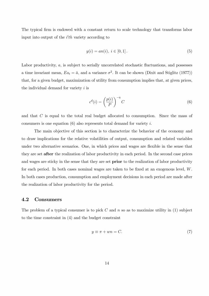
The typical firm is endowed with a constant return to scale technology that transforms labor

input into output of the i0th variety according to

y(i) = an(i), i ∈ [0, 1] . (5)

Labor productivity, a, is subject to serially uncorrelated stochastic fluctuations, and possesses

a time invariant mean, Eat =_a, and a variance σ2. It can be shown (Dixit and Stiglitz (1977))

that, for a given budget, maximization of utility from consumption implies that, at given prices,

the individual demand for variety i is

cd(i) =

µp(i)

P

¶−ηC (6)

and that C is equal to the total real budget allocated to consumption. Since the mass of

consumers is one equation (6) also represents total demand for variety i.

The main objective of this section is to characterize the behavior of the economy and

to draw implications for the relative volatilities of output, consumption and related variables

under two alternative scenarios. One, in which prices and wages are flexible in the sense that

they are set after the realization of labor productivity in each period. In the second case prices

and wages are sticky in the sense that they are set prior to the realization of labor productivity

for each period. In both cases nominal wages are taken to be fixed at an exogenous level, W .

In both cases production, consumption and employment decisions in each period are made after

the realization of labor productivity for the period.

4.2 Consumers

The problem of a typical consumer is to pick C and n so as to maximize utility in (1) subject

to the time constraint in (4) and the budget constraint

y ≡ π + wn = C. (7)

14

Here w ≡ WPand π are the real wage and the profits that the individual obtains from his share

of firms’ ownership. The individual consumes all his income. All profits are distributed to

individuals but they take them as given when choosing labor supply and consumption. Note

that since the mass of consumers is one, equation (7) represents the income, the consumption

and the functional income shares of a single individual, as well as the aggregate values of those

variables. The first order condition for the consumer problem is given by

wu0(π + wns)− v0(1− ns) = 0 (8)

and it implicitly determines labor supply, ns. It restates the conventional result that the individ-

ual works up to the point at which the marginal utility of an additional unit of time allocated

to work equals the marginal utility of leisure.

4.3 The flexible price and wage equilibrium (FPE)

The distinguishing feature of the FPE is that individual firms set their prices for each period

after the realization of labor productivity for the period.

4.3.1 Firms

The typical firm takes the general price level, total expenditure on consumption in (2) and (3)

and the known realization of productivity as given and sets its price so as to maximize the value

of profits. Real profits of each firm are given by

p(i)cd(i)−Wnd(i)P

=C

P 1−η

·(p(i))1−η − W

a(p(i))−η

¸. (9)

Here nd(i) = cd(i)ais the firm’s derived demand for labor needed to satisfy product demand at

level cd(i). Technically, the term to the right of the equality sign follows by using (5) and (6) to

substitute cd(i) and nd(i) out. Since the single firm takes C and P andW as given maximization

of (9) with respect to p(i) is equivalent to maximization of the term in brackets on the right

15

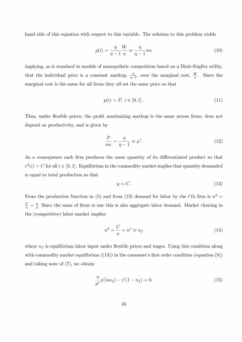
hand side of this equation with respect to this variable. The solution to this problem yields

p(i) =η

η − 1W

a≡ η

η − 1mc (10)

implying, as is standard in models of monopolistic competition based on a Dixit-Stiglitz utility,

that the individual price is a constant markup, ηη−1 , over the marginal cost,

Wa. Since the

marginal cost is the same for all firms they all set the same price so that

p(i) = P, i ∈ [0, 1] . (11)

Thus, under flexible prices, the profit maximizing markup is the same across firms, does not

depend on productivity, and is given by

P

mc=

η

η − 1 ≡ µ∗. (12)

As a consequence each firm produces the same quantity of its differentiated product so that

cd(i) = C for all i ∈ [0, 1] . Equilibrium in the commodity market implies that quantity demandedis equal to total production so that

y = C. (13)

From the production function in (5) and from (13) demand for labor by the i’th firm is nd =Ca= y

a. Since the mass of firms is one this is also aggregate labor demand. Market clearing in

the (competitive) labor market implies

nd =C

a= ns ≡ nf (14)

where nf is equilibrium labor input under flexible prices and wages. Using this condition along

with commodity market equilibrium ((13)) in the consumer’s first order condition (equation (8))

and taking note of (7), we obtain

a

µ∗u0(anf)− v0(1− nf) = 0. (15)

16

This relation implicitly determines the general equilibrium level of employment under flexible

prices.

Combining (10) and (11), the real wage under flexible prices is a constant multiple of

labor productivity and is given by

w ≡ WP=a

µ∗=

η − 1ηa. (16)

Thus, the real wage depends only on labor productivity and on the profit maximizing markup

of firms since, for any given nominal wage, W , firms always adjust their prices to obtain the

profit maximizing markup, µ∗.16 Given this real wage, clearing of the labor market is assured

by equation (15) that combines the first order condition of a representative individual with

labor market clearing. Essentially, labor market clearing is assured by the requirement that the

marginal utility of labor supplied is equal to the real wage multiplied by the marginal utility of

the consumption that is produced with this labor.

4.4 The sticky price and wage equilibrium (SPE)

Sticky prices and wages are characterized by the requirement that the nominal wage and prices

are set prior to the realization of labor productivity. As a consequence the real wage is invariant

to productivity shocks while the markup, which was invariant to those shocks under flexible

prices and wages, varies with the realization of productivity. But, production, employment and

consumption decisions are still made after the realization of each period’s shock.

4.4.1 Firms

The typical firm takes the general price level, total expenditure on consumption and the nominal

wage as given and sets its price so as to maximize the expected value of profits for the period.

The markup is uncertain now since the firm has to commit to a nominal price prior to the

realization of labor productivity. The firm picks its price at the beginning of each period so as

16As a consequence the nominal wage is inconsequential and can be taken as an arbitrary numeraire. Putdifferently, the equilibrium in the text pins down the real wage but not the nominal wage and the price level. .

17

to maximize

EC

P 1−η

·(p(i))1−η − W

a(p(i))−η

¸=

1

P 1−η£EC(p(i))1−η −WE(n)(p(i))−η¤ (17)

where the term to the right of the equality sign is obtained by using equations (9) and (14).

Note that at the time p(i) is chosen C and n are stochastic variables since they depend on the

yet unknown realization of labor productivity for the period. The solution to this problem is

p(i) =WE(n)

EC

η

η − 1 =WE(n)

ECµ∗ = P, i ∈ [0, 1] (18)

where the second equality follows from the definition of µ∗ in (12). The third equality reflects the

fact that all firms set the same price. Rearrangement of (18) provides an expression for the real

wage in terms of the, shock invariant, expected values of consumption and of employment.and

of the profit maximizing markup.

W

P=EC

En

1

µ∗≡ ws. (19)

Since both prices and wages are sticky the real wage remains at ws even after the realization of

productivity for the period implying that markups move up and down with productivity. The

precise relation is given by

µ(a) =a

ws. (20)

Similarly to the case of flexible prices and wages, the equilibrium conditions in the commodity

and the labor markets, along with the consumer’s first order condition in equation (8) imply

that equilibrium employment under sticky prices, ns, is determined implicitly from the relation

wsu0(ans)− v0(1− ns) = 0. (21)

18

4.5 Comparison of economic behavior under sticky and under flexi-

ble prices and wages

Equations (15) and (21) above can now be used to find the main differences between the behavior

of equilibrium employment under flexible and under sticky prices. Comparison of those equations

suggests that the only difference between them concerns the real wage. Under flexible prices

the real wage changes directly with productivity according to the relation wf = aµ∗ while, under

sticky prices it is fixed at ws. Clearly, for the particular productivity realization at which those

two real wages are equal the levels of employment in the two regimes are identical (nf = ns ≡ n).Denoting by a0 this particular level of productivity, a0 is determined by the relation

ws =a0µ∗≡ wf(a0). (22)

I turn next to the implications of the difference in real wage behavior for the behavior of

employment and of consumption. The following two propositions summarize the main results

Proposition 1 In the neighborhood of a0;

(i) A decrease in productivity raises employment under sticky prices and wages and raises

it under flexible prices and wages as well if the degree of relative risk aversion in consumption

(γ) is larger than one.

(ii) When γ is larger than one employment and leisure under sticky prices and wages are

more volatile than under flexible prices and wages.

(iii) When γ ≤ 1 a decrease in productivity lowers (or does not change) employment

under flexible prices and wages.17

Proposition 2 In the neighborhood of a0 consumption and output are positively related to pro-

ductivity under both flexible and sticky prices and wages but it fluctuates more widely in the first

case.

The proofs of the propositions are in the appendix.

17In this case a drop in productivity leads to a drop (if γ < 1) in employment under flexible prices and wages,exacerbating the effect of the decrease in productivity on consumption and to no change in it when γ = 1.

19

Intuitively, the basic reason for the differences between the two regimes is that, under

sticky prices and wages, the real wage does not adjust to changes in productivity, whereas it

changes directly with productivity under flexible prices and wages. But in both cases profits

(which individuals take as given) go up and down with productivity. As a consequence, in the

case of sticky prices and wages, the decrease in productivity, by reducing profits, triggers only

a (positive) wealth effect on employment.

In the case of flexible prices and wages the decrease in productivity also reduces the real

wage triggering additionally the familiar negative substitution and positive income effects of a

change in the real wage on employment. If the degree of relative risk aversion in consumption

is sufficiently large (γ > 1) the positive wealth and income effects dominate the negative sub-

stitution effect and employment moves to partially offset the effect of the productivity decrease

on consumption also under flexible prices and wages.18 Due to the positive correlation between

the real wage and productivity under flexible prices and wages the offset is smaller in this case.

The second proposition is a corrolary of the first. The relatively smaller increase in employment

following a decrease in productivity under flexible prices and wages offsets the drop in consump-

tion to a lesser extent than under sticky prices and wages.19 As a consequence, consumption

and output fluctuate more and, for γ > 1, employment and leisure fluctuate less under flexible

prices and wages.

4.6 A reinterpretation of the analysis

This subsection argues that the analysis presented so far can also be reinterpreted as a compari-

son between sticky and flexible prices given that the nominal wage is sticky in both cases. Such

a reinterpretation is useful because wages are normally believed to be more sticky than most

prices20. Recent evidence from a detailed study of the Belgian CPI during the nineties suggests

that more than fivty percent of individual prices have a duration lower than one year (Figure 1

18In the special case γ = 1 the positive substitution effect and the sum of the negative income and wealtheffects exactly offset each other so that a change in productivity does not affect employment under flexible pricesand wages.19As a matter of fact when γ < 1 this effect is even stronger since a decrease in productivity reduces employment

under flexible prices and wages exacerbating the decrease in consumption due to the decrease in productivity.20See Friedman (1999) for example.

20

in Aucremanne and Dhyne (2004)). Since the duration of nominal wage contracts is normally

at least a year prices appear to be generally more flexible than nominal wages.21 It is therefore

of some interest to contrast the behavior of the economy under sticky and under flexible prices

given a sticky nominal wage.

To establish the claim at the beginning of this subsection we only need to show that the

equilibrium obtained in the case of flexible prices and wages is identical to an equilibrium in

which the nominal wage is preset at some arbitrary level prior to the realization of productivity

and in which prices are set after productivity is revealed to firms.22 This follows in turn from

the observation that, independently of whether the nominal wage is preset or is determined

after the realization of productivity, firms always adjust prices under flexible prices so that

the profit maximizing markup is µ∗. It follows, from equation (12) that, whatever the nominal

wage, the real wage is given by equation (16). Competitive clearing of the labor market implies

that equation (14) holds and equilibrium in the goods’ market implies equation (13) again.

Substituting those relations into the consumer - worker first order condition in equation (8)

leads again to equation (15) which yields the same general equilibrium level of employment as

in the case of flexible prices and wages. The other equations then also produce identical levels

of production and profits.

Thus the main comparison in which the real equilibrium under sticky prices and wages

is contrasted with the equilibrium under flexible values of those variables is equivalent to the

case in which it is compared to a benchmark with flexible prices and a sticky nominal wage.

5 Implications for relative welfare under sticky and un-

der flexible prices and wages

A widely used criterion for the exante evaluation of welfare is expected utility. Risk averse

individuals prefer stable consumption and stable leisure to fluctuating values of those variables.

The two propositions above imply that (in the neighborhood of a0) consumption is more volatile,

21See also Bewley (1999) for the US. A survey of recent models in which prices are more flexible than nominalwages appears in Cukierman (2004).22The sticky price and wage equilibrium is obviously the same.

21

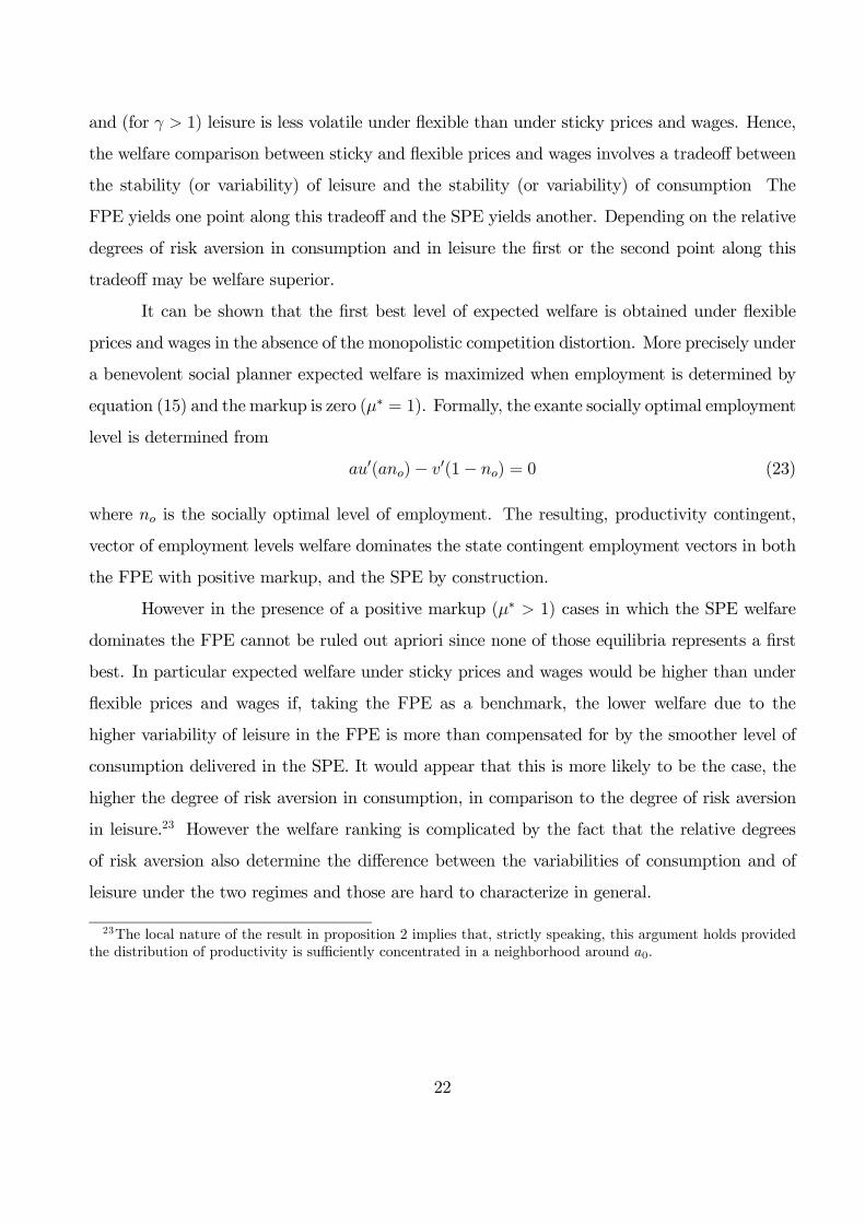
and (for γ > 1) leisure is less volatile under flexible than under sticky prices and wages. Hence,

the welfare comparison between sticky and flexible prices and wages involves a tradeoff between

the stability (or variability) of leisure and the stability (or variability) of consumption The

FPE yields one point along this tradeoff and the SPE yields another. Depending on the relative

degrees of risk aversion in consumption and in leisure the first or the second point along this

tradeoff may be welfare superior.

It can be shown that the first best level of expected welfare is obtained under flexible

prices and wages in the absence of the monopolistic competition distortion. More precisely under

a benevolent social planner expected welfare is maximized when employment is determined by

equation (15) and the markup is zero (µ∗ = 1). Formally, the exante socially optimal employment

level is determined from

au0(ano)− v0(1− no) = 0 (23)

where no is the socially optimal level of employment. The resulting, productivity contingent,

vector of employment levels welfare dominates the state contingent employment vectors in both

the FPE with positive markup, and the SPE by construction.

However in the presence of a positive markup (µ∗ > 1) cases in which the SPE welfare

dominates the FPE cannot be ruled out apriori since none of those equilibria represents a first

best. In particular expected welfare under sticky prices and wages would be higher than under

flexible prices and wages if, taking the FPE as a benchmark, the lower welfare due to the

higher variability of leisure in the FPE is more than compensated for by the smoother level of

consumption delivered in the SPE. It would appear that this is more likely to be the case, the

higher the degree of risk aversion in consumption, in comparison to the degree of risk aversion

in leisure.23 However the welfare ranking is complicated by the fact that the relative degrees

of risk aversion also determine the difference between the variabilities of consumption and of

leisure under the two regimes and those are hard to characterize in general.

23The local nature of the result in proposition 2 implies that, strictly speaking, this argument holds providedthe distribution of productivity is sufficiently concentrated in a neighborhood around a0.

22

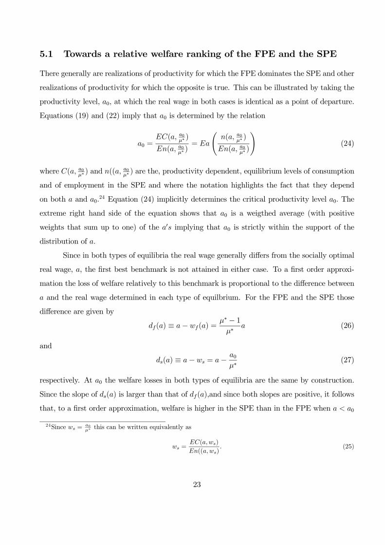
5.1 Towards a relative welfare ranking of the FPE and the SPE

There generally are realizations of productivity for which the FPE dominates the SPE and other

realizations of productivity for which the opposite is true. This can be illustrated by taking the

productivity level, a0, at which the real wage in both cases is identical as a point of departure.

Equations (19) and (22) imply that a0 is determined by the relation

a0 =EC(a, a0

µ∗ )

En(a, a0µ∗ )

= Ea

Ãn(a, a0

µ∗ )

En(a, a0µ∗ )

!(24)

where C(a, a0µ∗ ) and n((a,

a0µ∗ ) are the, productivity dependent, equilibrium levels of consumption

and of employment in the SPE and where the notation highlights the fact that they depend

on both a and a0.24 Equation (24) implicitly determines the critical productivity level a0. The

extreme right hand side of the equation shows that a0 is a weigthed average (with positive

weights that sum up to one) of the a0s implying that a0 is strictly within the support of the

distribution of a.

Since in both types of equilibria the real wage generally differs from the socially optimal

real wage, a, the first best benchmark is not attained in either case. To a first order approxi-

mation the loss of welfare relatively to this benchmark is proportional to the difference between

a and the real wage determined in each type of equilbrium. For the FPE and the SPE those

difference are given by

df(a) ≡ a− wf(a) = µ∗ − 1µ∗

a (26)

and

ds(a) ≡ a− ws = a− a0µ∗

(27)

respectively. At a0 the welfare losses in both types of equilibria are the same by construction.

Since the slope of ds(a) is larger than that of df(a),and since both slopes are positive, it follows

that, to a first order approximation, welfare is higher in the SPE than in the FPE when a < a0

24Since ws = a0µ∗ this can be written equivalently as

ws =EC(a,ws)

En((a,ws). (25)

23

and that the opposite holds when a > a0. Since the difference in expected welfare between the

SPE and the FPE is a probability weighted average of such differences for given values of a it

would appear that there generally exist utility specifications and probability distributions for

which this difference may be of either sign. However experimentation with several alternative

specifications of utility limited by the requirement that employment levels are solvable explicitly

from the appropriate first order conditions revealed that, at least within this set, there is a

predominance of cases in which expected welfare is higher under the FPE. Details appear in

subsections 5.3 and 5.4 below.

Those findings raise two questions. One concerns the very existence of cases in which

the SPE delivers a higher level of welfare than the FPE. The other concerns the derivation of

conditions that allow a sharper discrimination between cases in which expected welfare in the

SPE is higher than in the FPE from cases in which the opposite is true. The next subsection

produces a case in which the SPE welfare dominates the FPE implying that the set of cases in

which sticky prices and wages provide a higher level of expected welfare than flexible prices and

wages is non empty. The subsequent subsection derives conditions on utilities and on probability

distributions of productivity shocks that provide a sharper perspective on some of the factors

that determine which of the two types of equilibria is welfare superior.

5.2 Demonstration that the set of cases in which expected welfare

in the SPE is higher than in the FPE is non empty

Let

∆(a) ≡ u(Cs(a)) + v(ls(a))− {u(Cf(a)) + v(lf(a))} (28)

where Cs(a) = C(a, a0µ∗ ) and ls(a) are equilibrium consumption and leisure in the SPE and Cf(a)

and lf(a) are equilibrium consumption and leisure in the FPE. Expected welfare under a SPE

is higher if and only if

E∆(a) > 0. (29)

The following subsubsection presents a specific numerical example in which this is the case.

24

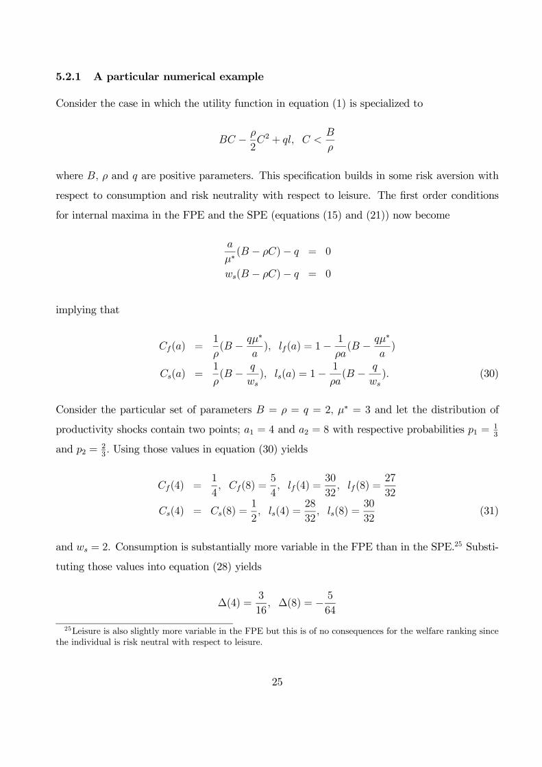
5.2.1 A particular numerical example

Consider the case in which the utility function in equation (1) is specialized to

BC − ρ

2C2 + ql, C <

B

ρ

where B, ρ and q are positive parameters. This specification builds in some risk aversion with

respect to consumption and risk neutrality with respect to leisure. The first order conditions

for internal maxima in the FPE and the SPE (equations (15) and (21)) now become

a

µ∗(B − ρC)− q = 0

ws(B − ρC)− q = 0

implying that

Cf(a) =1

ρ(B − qµ

∗

a), lf(a) = 1− 1

ρa(B − qµ

∗

a)

Cs(a) =1

ρ(B − q

ws), ls(a) = 1− 1

ρa(B − q

ws). (30)

Consider the particular set of parameters B = ρ = q = 2, µ∗ = 3 and let the distribution of

productivity shocks contain two points; a1 = 4 and a2 = 8 with respective probabilities p1 = 13

and p2 = 23. Using those values in equation (30) yields

Cf(4) =1

4, Cf(8) =

5

4, lf(4) =

30

32, lf(8) =

27

32

Cs(4) = Cs(8) =1

2, ls(4) =

28

32, ls(8) =

30

32(31)

and ws = 2. Consumption is substantially more variable in the FPE than in the SPE.25 Substi-

tuting those values into equation (28) yields

∆(4) =3

16, ∆(8) = − 5

64

25Leisure is also slightly more variable in the FPE but this is of no consequences for the welfare ranking sincethe individual is risk neutral with respect to leisure.

25

which implies that

E∆(a) =1

96> 0.

Thus the SPE, with its relatively smoother levels of consumption and of output, welfare domi-

nates the FPE. Continuity considerations and simulations (not shown) suggest that this case is

not an isolated one.

5.3 The class of utilities functions u(C) + v(l) = C1−γ1−γ + ql

Here u(C) is a CRRA in consumption and γ and q are positive parameters. This is a convenient

case since its equilibrium can be obtained explicitly from the first order conditions in equations

(15) and (21). The equilibrium values of consumption and of leisure under flexible and under

sticky prices are given respectively by

Cf =

µa

qµ∗

¶ 1γ

, lf = 1−µ1

qµ∗

¶ 1γ

a1−γγ

Cs =

µwsq

¶ 1γ

, ls = 1−µwsq

¶ 1γ 1

a

where

ws =1

µ∗E 1a

.

Proposition 3 For the family of utility functions, u(c)+v(l) = c1−γ1−γ +ql, expected welfare under

flexible prices and wages is larger than expected welfare under sticky prices and wages for all

possible markups and distributions of productivity shocks.

The proof of the proposition appears in Cukierman and Shapir (2005).

5.4 The cases u(C) + v(l) = lnC + ln l and u(C) + v(l) = − 1C + ln l

Those cases too lead to explicit analytical solutions which can be used to calculate expected

welfare in both regimes as functions of basic parameters for given distributions of productivity

shocks. An extensive grid search over alternative combinations of the markup with uniform,

triangular and truncated normal distributions of productivity shocks with varying supports

26

indicate that, in all cases, expected welfare under flexible prices and wages is higher than under

sticky prices and wages.

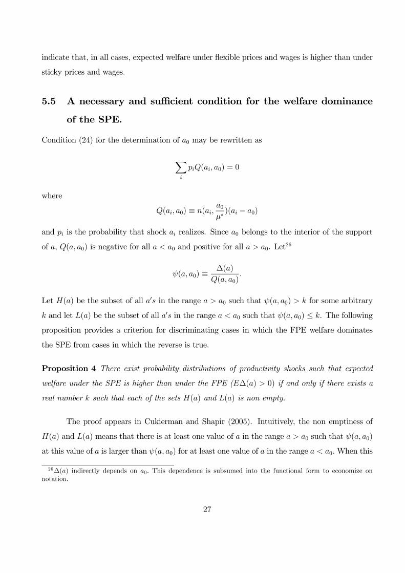
5.5 A necessary and sufficient condition for the welfare dominance

of the SPE.

Condition (24) for the determination of a0 may be rewritten as

Xi

piQ(ai, a0) = 0

where

Q(ai, a0) ≡ n(ai, a0µ∗)(ai − a0)

and pi is the probability that shock ai realizes. Since a0 belongs to the interior of the support

of a, Q(a, a0) is negative for all a < a0 and positive for all a > a0. Let26

ψ(a, a0) ≡ ∆(a)

Q(a, a0).

Let H(a) be the subset of all a0s in the range a > a0 such that ψ(a, a0) > k for some arbitrary

k and let L(a) be the subset of all a0s in the range a < a0 such that ψ(a, a0) ≤ k. The followingproposition provides a criterion for discriminating cases in which the FPE welfare dominates

the SPE from cases in which the reverse is true.

Proposition 4 There exist probability distributions of productivity shocks such that expected

welfare under the SPE is higher than under the FPE (E∆(a) > 0) if and only if there exists a

real number k such that each of the sets H(a) and L(a) is non empty.

The proof appears in Cukierman and Shapir (2005). Intuitively, the non emptiness of

H(a) and L(a) means that there is at least one value of a in the range a > a0 such that ψ(a, a0)

at this value of a is larger than ψ(a, a0) for at least one value of a in the range a < a0.When this

26∆(a) indirectly depends on a0. This dependence is subsumed into the functional form to economize onnotation.

27

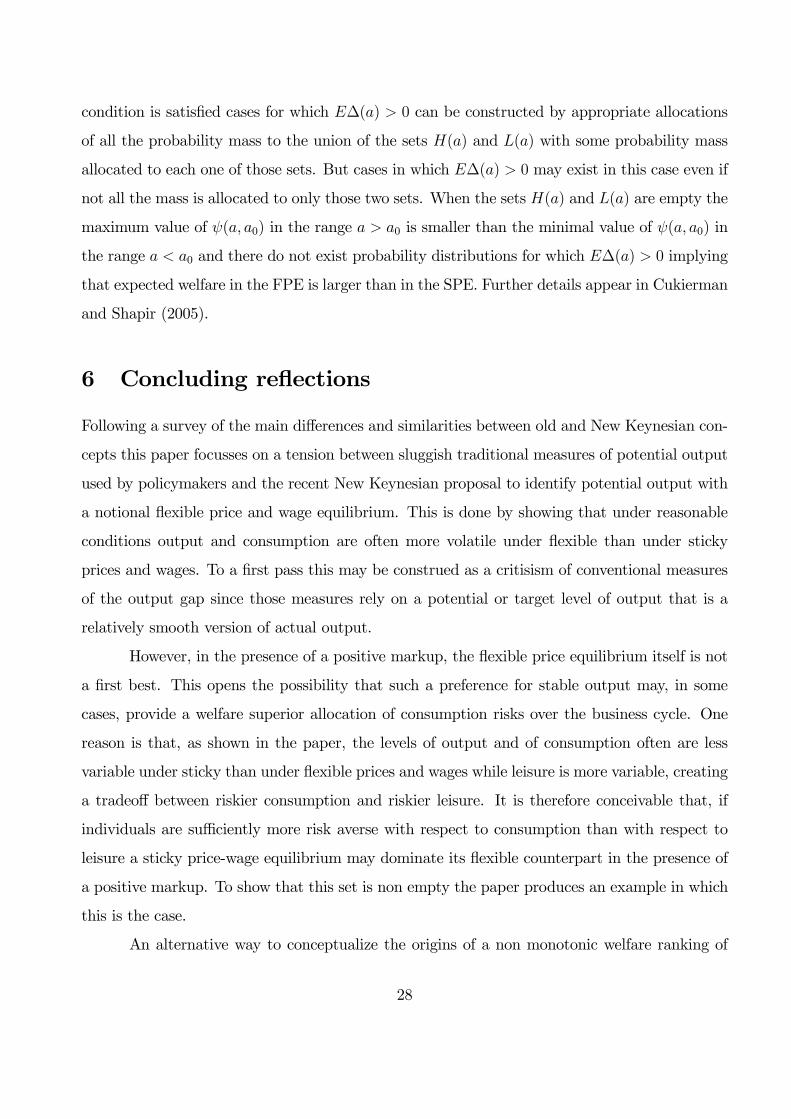
condition is satisfied cases for which E∆(a) > 0 can be constructed by appropriate allocations

of all the probability mass to the union of the sets H(a) and L(a) with some probability mass

allocated to each one of those sets. But cases in which E∆(a) > 0 may exist in this case even if

not all the mass is allocated to only those two sets. When the sets H(a) and L(a) are empty the

maximum value of ψ(a, a0) in the range a > a0 is smaller than the minimal value of ψ(a, a0) in

the range a < a0 and there do not exist probability distributions for which E∆(a) > 0 implying

that expected welfare in the FPE is larger than in the SPE. Further details appear in Cukierman

and Shapir (2005).

6 Concluding reflections

Following a survey of the main differences and similarities between old and New Keynesian con-

cepts this paper focusses on a tension between sluggish traditional measures of potential output

used by policymakers and the recent New Keynesian proposal to identify potential output with

a notional flexible price and wage equilibrium. This is done by showing that under reasonable

conditions output and consumption are often more volatile under flexible than under sticky

prices and wages. To a first pass this may be construed as a critisism of conventional measures

of the output gap since those measures rely on a potential or target level of output that is a

relatively smooth version of actual output.

However, in the presence of a positive markup, the flexible price equilibrium itself is not

a first best. This opens the possibility that such a preference for stable output may, in some

cases, provide a welfare superior allocation of consumption risks over the business cycle. One

reason is that, as shown in the paper, the levels of output and of consumption often are less

variable under sticky than under flexible prices and wages while leisure is more variable, creating

a tradeoff between riskier consumption and riskier leisure. It is therefore conceivable that, if

individuals are sufficiently more risk averse with respect to consumption than with respect to

leisure a sticky price-wage equilibrium may dominate its flexible counterpart in the presence of

a positive markup. To show that this set is non empty the paper produces an example in which

this is the case.

An alternative way to conceptualize the origins of a non monotonic welfare ranking of

28

sticky and flexible nominal price regimes is to note that in both of them the average renumeration

to labor is too low in comparison to the first best. But, since the real wage is fixed in the first case

and variable in the second, the first regime welfare dominates the second.for some realizations

of productivity shocks while the opposite is true for other realizations.

Thus targeting the flexible price and wage equilibrium (as recommended in the main

part of Woodford (2003, chapter 6)) might be abstracting from welfare considerations that go

beyond the relative price distortions featured in recent NKM. One may wonder about the origin

of the difference between this view and the discussion in this paper. Woodford derives his

result under the assumption that there is in place a system of taxes cum subsidies that offset

the monopolistic competition distortion. By contrast, the framework of this paper compares a

regime featuring sticky nominal variables with its flexible counterpart in the presence of a

monopolistic competition distortion.27

It is instructive to compare the broad conclusions obtained here with those of Goodfriend

and King (1997) and Goodfriend (2002) in their new neoclassical synthesis. They postulate that

prices are sticky but that nominal wages are flexible. As a consequence, an unanticipated

productivity shock is equilibrated by changes in the nominal wage and individuals work less in

periods of low productivity exacerbating the fall in consumption, due to the reduced productivity.

By contrast, as shown here, when both wages and prices are sticky, individuals work more in

periods of low productivity. This partially shields consumption from the wider fluctuations

produced under flexible prices and wages.

The paper also briefly discusses more general necessary and sufficient conditions for a

sticky price and wage equilibrium to welfare dominate its flexible counterpart. These conditions

in conjunction with some additional examples indicate that the set of cases in which the flexible

price and wage equilibrium dominates its sticky counterpart is likely to be larger than the set for

which the opposite is true. Thus, although the welfare dominance of sticky nominal variables

cannot be excluded, there are important classes of cases in which flexible prices and wages

welfare dominate sticky prices and wages in spite of the presence of a monopolistic competition

27Benigno and Woodford (2004) have recently extended the analysis of optimal monetary policy to the casein which there is a monopolistic competition distortion. Khan King and Wolman (2003) characterize optimalmonetary policy in the presence of monopolistic competition, price stickiness and costly conversions of wealthinto goods.

29

distortion. Finding a sharper demarcation line between those two sets is left for future work.

7 Appendix:

7.1 Proof of proposition 1

(i) Applying the implicit function theorem to equations (15) and (21) to evaluate the effects of

a change in a on the equilibrium level of employment in the neighborhood of a0 yields

dnfda(a0) = −

nwsu”(a0n) +1µ∗u

0(a0n)

a0wsu”(a0n) + v”(1− n) (32)

dnsda(a0) = − nwsu”(a0n)

a0wsu”(a0n) + v”(1− n) . (33)

The denominators of both expressions are identical and (since u”(.) < 0 and v”(.) < 0) negative.

Since both expressions are preceded by minus signs their signs are determined by the signs of

their respective numerators. Hence (since u”(.) < 0) the sign of dnsda(a0) is negative but (since

1µ∗u

0(.) > 0) the sign of dnfda(a0) is generally ambiguous. Employment goes up following a

decrease in productivity, under flexible prices, if and only if the numerator of equation (32) is

negative.Using equation (22) to substitute ws out from this numerator this is the case, in turn,

if and only if

cfu”(cf) + u0(cf) < 0. (34)

Rearranging, this is equivalent to

(1− γ)u0(cf) < 0 (35)

where

γ ≡ −cfu”(cf)u0(cf)

is the coefficient of relative risk aversion in consumption. It is easily seen that condition (35) is

equivalent to the condition γ > 1. Hence a decrease in productivity raises employment under

both sticky and flexible prices.

30

(ii) Comparison of equations (32) and (33) reveals (since 1µ∗u

0(.) > 0) that

dnsda(a0) <

dnfda(a0) < 0 (36)

where the second inequality is implied by part (i) and the condition γ > 1. Hence employment

and leisure are more volatile under sticky than under flexible prices.

(iii) The condition γ ≤ 1 is equivalent to

cfu”(cf) + u0(cf) ≤ 0

which implies, from equation (32), that dnfda(a0) ≥ 0.

7.2 Proof of proposition 2

The constant return to scale technology in conjunction with equilibrium in the commodity

market imply that, for any a,

C = an(a) (37)

where the notation n(a) highlights the fact that the level of employment depends on productivity.

Differentiating equation (37) with respect to a

dC

da(a) = n(a) + a

dn

da(a). (38)

Substituting dnsda(a0) into equation (38) and rearranging

dCsda(a) =

nv”(a0n)

a0wsu”(a0n) + v”(1− n) > 0. (39)

Thus, in spite of a stronger offsetting effect via employment under sticky than under flexi-

ble prices, consumption goes up and down with productivity in the sticky prices case. Using

equations (36) and (39) in (38) yields

0 <dCsda(a) <

dCfda(a)

31

implying that, under both sticky and flexible prices, consumption is directly related to produc-

tivity, and that it fluctuates more widely under the latter.

8 References

Artis M., M. Marcellino and T. Proietti (2003), ”Dating the European Business Cycle”, CEPR

DP No. 3696, January.

Aucremanne L. and E. Dhyne (2004), ”How Frequently Do Prices Change? Evidence

Based on the Micro Data Underlying the Belgian CPI”, Paper presented at the May 2004

ESSIM, Tarragona, Spain.

Benigno P. and M. Woodford (2004), ”Optimal Stabilization Policy When Wages and

Prices are Sticky: The Case of a Distorted Steady State”, Manuscript, July.

Bewley T. (1999),Why Wages Don’t Fall During a Recession, Harvard University

Press, Cambridge, Mass.

Blanchard O. and Kiyotaki N. (1987), ”Monopolistic Competition and the Effects of

Aggregate Demand”, American Economic Review, 77, 647-666, September.

Calvo G. (1983), ”Staggered Price setting in a Utility-Maximizing Framework”, Journal

of Monetary Economics, 12, 383-398.

Clarida R., J. Gali and M. Gertler (1999). ”The Science of Monetary Policy: a New

Keynesian Perspective”, Journal of Economic Literature, 37, December, 1661-1707.

Cukierman A. (1983), ”Relative Price Variability and Inflation - A Survey and Further

Results,” in K. Brunner and A. Meltzer (eds.), Variability in Employment Prices and Money,

Carnegie-Rochester Conference Series on Public Policy, 19, Autumn , North-Holland,

Amsterdam, 103-158.

A. Cukierman, (2004), ”Monetary Institutions, Monetary Union and Unionized Labor

Markets - Some Recent Developments ”, in: Beetsma R., C. Favero, A. Missale, V.A. Muscatelli,

P. Natale and P. Tirelli (eds.), Monetary Policy, Fiscal Policies and Labour Markets:

Macroeconomic Policymaking in EMU , Cambridge University Press, Cambridge and NY.

Available on the web at: http://www.tau.ac.il/~alexcuk/pdf/milansurvey.pdf

Cukierman and Shapir (2005), ”Technical Appendix to: Keynesian Economics, Mon-

32

etary Policy and the Business Cycle - New and Old”, September. Available on the web at:

http://www.tau.ac.il/~alexcuk/pdf/cukierman-shapir-tech-app.pdf

Dotsey M. and R. King (2005), ”Implications of State-Dependent Pricing for Dynamic

Macroecononic Models”, Working Paper No. 05-2, Federal Reserve Bank of Philadelphia, Feb-

ruary.

Dixit A. and J. Stiglitz (1977), ”Monopolistic Competition and Optimal Product Diver-

sity”, American Economic Review, 67, 297-308.

Erceg C., D. Henderson and A. Levin (2000), ”Optimal Monetary Policy with Staggered

Wage and Price Contracts”, Journal of Monetary Economics, 46, 281-313.

Friedman B. (1999), "Comment on King and Wolman", in J. B. Taylor (ed.) Monetary

Policy Rules, The University of Chicago Press and NBER, Chicago and London, 398-402.

Friedman M. (1968), ”The Role of Monetary Policy”, American Economic Review,

58, 1-17.

Gali J. (2002), ”The Conduct of Monetary Policy in the Face of Technological Change:

Theory and Postwar US Evidence”, in Stabilization and Monetary Policy: the Interna-

tional Experience, Banco de Mexico, Mexico D. F.,

Gali J. (2003), ”New Perspectives on Monetary Policy, Inflation and the Business Cy-

cle”, in M. Dewatripont, L. Hansen and S. Turnovsky (eds.), Advances in Economics and

Econometrics, V. III, Cambridge University Press, Cambridge and NY, 151-197.

Goodfriend M. (2002), “Monetary Policy in the New Neoclassical Synthesis: A Primer”,

International Finance, 5(2) pp. 165-191.

Goodfriend M. and R. King (1997), ”The New Neoclassical Synthesis and the Role of

Monetary Policy”, NBER Macroeconomic Annual, MIT Press, Cambridge, Mass., 231-282.

Goodfriend M. and R. King (2001), "The Case for Price Stability", NBERWP No. 8423,

August.

Khan A., R. King and A. Wolman (2003), "Optimal Monetary Policy", Review of

Economic Studies, 70, issue 245, 825-860.

King R. and A. Wolman (1999), "What Should the Monetary Authority Do When Prices

Are Sticky?", in J. B. Taylor (ed.) Monetary Policy Rules, The University of Chicago Press

and NBER, Chicago and London, 349-398.

33

Lucas R. E. Jr. (1972), ”Expectations and the Neutrality of Money”, Journal of Eco-

nomic Theory, 4, 103-124.

Lucas R. E. Jr. (1973), ”Some International Evidence on Output-Inflation Tradeoffs”,

American Economic Review, 63, 326-335, June.

Mankiw G. and R. Reis (2002), ”Sticky Information Versus Sticky Prices: A Proposal to

Replace the New Keynesian Phillips Curve”, Quarterly Journal of Economics, 117, 1295-

1328, November.

Obstfeld M. and K. Rogoff (1995), ”Exchange Rate Dynamics Redux”, Journal of

Political Economy, 103, 624-660, June.

Phillips A. W. (1958), ”The Relation between Unemployment and the Rate of Change

of Money Wage Rates in the UK, 1861-1957”, Economica, 25, 283-299.

Rotemberg J. and M. Woodford (1997), ”An Optimization Based Econometric Frame-

work for the Evaluation of Monetary Policy”, In B. Bernanke and J. Rotemberg (eds.), NBER

Macroeconomic Annual, MIT Press, Cambridge, Mass., 297-346.

Samuelson P. A. and R. M. Solow (1960), ”Analytical Aspects of Anti-inflation Policy”,

Papers and Proceedings of the American Economic Association, 50, 177-194.

Schmitt-Grohe S. and M. Uribe (2004), ”Optimal Simple and Implementable Monetary

and Fiscal Rules”, Presented at a conference on Dynamic Macroeconomic Theory, University of

Copenhagen, June.

Sheshinski E. and Y. Weiss (eds.) (1993), Optimal Pricing, Inflation and Cost of

Price Adjustment, MIT Press, Cambridge, Mass.

Woodford M. (2003), Interest and Prices: Foundations of a Theory of Monetary

Policy, Princeton University Press, Princeton, NJ.

34