kevin doherty thesis - university digital conservancy home
TRANSCRIPT

University of Minnesota Graduate School
This is to certify that I have examined this copy of a master’s thesis by
Kevin Eric Doherty
And have found that it is complete and satisfactory in all respects, and that any and all revisions required by the final examining committee have been made
David E. Andersen
Signature of Faculty advisor
Date
Fall movements patterns of adult female American woodcock (Scolopax minor) in the western Great
Lakes region
A Thesis submitted to the faculty of the Graduate School of the University of Minnesota by
Kevin Eric Doherty
In partial fulfillment of the requirements for the degree of Master of Science
December 2004

i
TABLE OF CONTENTS Table of Contents……………………………………………………………….…… i Acknowledgements....................................................................................................iii List of Figures………………………………………………………………………..v List of Tables…………………………………………………………………….....vii List of Appendixes………………………………………………………………... viii CHAPTER 1
Effects of habitat and weather on the movement patterns of adult female American woodcock in the western Great Lakes region: Abstract……………………………………………………………………….......... 1 Introduction………………………………………………………………………… 2 Study Area…………………………………………………………………………. 4 Methods……………………………………………………………………………. 5 Capture and Radio Marking……………………………………………….. 5 Radio Tracking…………………………………………………………….. 5 Predictor Variables……………………………………………………........ 7 Movement Data……………………………………………………………. 8 A priori Models……………………………………………………………. 8 Data Analysis…………………………………………………………... 11 Results…………………………………………………………………………….. 13 Discussion………………………………………………………………………… 15 Literature Cited…………………………………………………………………… 18
CHAPTER 2
Fixed kernel home range estimation incorporating telemetry locational error: American woodcock (Scolopax minor) home range analysis using real and simulated data Abstract……………………………………………………………………………. 34 Introduction……………………………………………………………………….. 35 Study Area………………………………………………………………………… 37 Methods…………………………………………………………………………… 38 Capture and Radio Marking………………………………………………. 38 Radio Tracking……………………………………………………………. 38 Home Range Analysis…………………………………………………….. 39 Influence of Sample size..…………………………………………………. 40 Monte Carlo Home Range Simulation………….…………………………. 41 Influence of Sample size using Monte Carlo Simulations……………....... 41 Statistical comparisons……………………………………………………. 42

ii
Results…………………………………………………………………………….. 42 Woodcock Telemetry results....…………………………………………… 42 Monte Carlo Simulation results…………………………………………… 43 Discussion…………………………………………………………………………. 45 Literature Cited……………………………………………………………………. 48
iii
ACKNOWLEDGMENTS: My research is part of a large collaborative effort investigating woodcock
survival, habitat use, and movement in the western Great Lakes region. First, I would
like to thank 2 graduate students with whom I collaborated very closely during the
field seasons and who coordinated the collection of movement data for me for 2 years
on their respective study sites; Jed Meunier of the University of Wisconsin and Eileen
Oppelt of Northern Michigan University. I would also like to thank their major
professors and Co-PI's on the project John Bruggink of Northern Michigan University
and Scott Lutz of the University of Wisconsin. Last and by no means least I would
like to thank my major professor David Andersen. I would like to thank him for
sharing his patience, intellect, keen editorial skills, and passion for game birds with
me. This thesis would not be what it is without his mentoring. Everybody who has
worked for David has said the same; you really can't get a better boss. Finally, I
would like to thank him for showing me the world of pointing dogs. It's hard to beat
walking though the woods with your shotgun on a cool fall day hunting woodcock
and watching a bird dog work; especially if that's your lab meeting!
This project was funded by the U.S. Fish and Wildlife Service, Region 3; U.S.
Geological Survey (Science Support Initiative); Wisconsin Department of Natural
Resources; Minnesota Department of Natural Resources; Michigan Department of
Natural Resources; the 2001 Webless Migratory Game Bird Research Program;
University of Wisconsin-Madison; University of Minnesota-Twin Cities; Northern
Michigan University; the Minnesota Cooperative Fish and Wildlife Research Unit;
the Ruffed Grouse Society; Wisconsin Pointing Dog Association; and the North
Central Wisconsin Chapter of the North American Versatile Hunting Dog
Association. We thank D.G. McAuley for helping with identifying mist-netting and
night-lighting sites and suggestions for techniques for handling woodcock. On the
Minnesota study site, special thanks are due Dick Tuszynski, Craig Kostrzewski,
Steve Piepgras, Jeremy Abel, Richard "Zeke" Black, and Tim Pharis for assistance
with various aspects of field work and Mike Trentholm for locating missing birds by

iv
aerial telemetry. On the Michigan study site, we thank D.E. Beyer for the Michigan
Department of Natural Resources for coordinating telemetry flights.

v
LIST OF FIGURES: CHAPTER 1 Fig. 1. Location of study areas in Minnesota, Wisconsin, and Michigan where American woodcock were radio-marked during the falls of 2002 and 2003........... 23 Fig. 2. Distance between subsequent locations (n = 1,786) for radio-tagged female after-hatch-year American woodcock (n = 58) during falls of 2002 and 2003 in Minnesota, Wisconsin, and Michigan………………………………...…………… 24 CHAPTER 2 Fig. 1. Standardized (probability area at n / largest 95% probability area) woodcock 95% probability areas (solid line) and 50% probability areas (dashed line) using hlscv and her as the smoothing parameter in a fixed kernel in relation to sample size. Location data are from after-hatch-year female woodcock (n = 7) in east-central Minnesota during the fall of 2003….................................................................................................................................. 51 Fig. 2. Mean and range of the coefficient of variation vs. sample size for the 50% and 95% probability areas of fixed kernels using both hlscv (white diamond/dashed line) and her (black diamond/solid line), derived from telemetry data from after-hatch-year female American woodcock in east-central Minnesota in the fall of 2003. Two hundred bootstrap samples per sample size were analyzed for each of 7 woodcock………………………………………. 52 Fig. 3. Ninety-five percent CIs of bootstrapped fixed kernel means and kernel probability estimates (using her [black diamond] and hlscv [white diamond]) for 95% and 50% probability areas for after-hatch-year female American woodcock in east-central Minnesota in 2003.... …………………………………………………………………………………………….. 53 Fig. 4. Ninety-five percent CIs of bootstrapped fixed kernel means and kernel probability estimates for 95% and 50% probability areas using her (black diamond) and hlscv (white diamond) for after-hatch-year female American woodcock in east-central Minnesota in 2003. …………………………………………………………………………………...... 54 Fig. 5. Mean size and 95% CIs of bootstrap mean (dashed lines) of the 95% (black diamond) and 50% (black square) probability area of fixed kernels using hlscv and her as the bandwidth selection method, on a simulated woodcock home range with 1 core use area. True area is represented by dark black line. Data are from 200 bootstrap samples per sample size….. 55 Fig. 6. Coefficient of variation vs. sample size for the 95% and 50% probability areas of fixed kernels using both hlscv (dashed line) and her (solid line) for simulated woodcock home ranges with; 1 core use area, 1 core use area distant from a single satellite area of infrequent use, and 2 core use areas. True area is represented by dark black line. Data are based on 200 bootstrap samples per sample size………………………………………………………… 56
vi
Fig. 7. Mean size and 95% CIs of bootstrap mean (dashed lines) of the 95% (black diamond) and 50% (black square) probability area of fixed kernels using hlscv and her as the bandwidth selection method, on a simulated woodcock home range with 1 core use area distant from a single satellite area of infrequent use. True area is represented by dark black line. Data are from 200 bootstrap samples per sample size…………………………………………........ 57 Fig. 8. Mean size and 95% CIs of bootstrap mean (dashed lines) of the 95% (black diamond) and 50% (black square) probability area of fixed kernels using hlscv and her as the bandwidth selection method, on a simulated woodcock home range with 2 use areas. True area is represented by dark black line. Data are from 200 bootstrap samples per sample size…... 58 Fig. 9. Mean and 95% CIs of the percent of simulated home range area estimated using fixed kernels (95% probability area) with her and hlscv as the bandwidth selection method in relation to varying spatial orientations. Data are from 500 Monte Carlo simulated home ranges of n = 50 for each polygon type and smoothing method…………………………………………. 59

vii
LIST OF TABLES: CHAPTER 1 Table 1. American woodcock movement predictor variables and covariates at locations determined via radio telemetry in 2002 and 2003, in central Minnesota, central Wisconsin, and the Upper Peninsula of Michigan………………...……… 25 Table 2. Descriptive statistics of predictor variables and distances between subsequent locations (n = 1,786) of after-hatch-year female American woodcock (n = 58) in central Minnesota, central Wisconsin, and the Upper Peninsula of Michigan during the falls of 2002 and 2003.…………………...............…………. 26 Table 3. Effects of blocking on process variation explained and summary of best models (n = 5 of 27 a priori models) and means model predicting distances between subsequent daily locations of after-hatch-year female American woodcock (n = 58) in central Minnesota, central Wisconsin, and the Upper Peninsula of Michigan during the falls of 2002 and 2003.…………………………….…………………………... 27 Table 4. Regression coefficient estimates and associated standard errors for the distance between subsequent daily locations of after-hatch-year female American woodcock in central Minnesota, central Wisconsin, and the Upper Peninsula of Michigan during the falls of 2002 and 2003. Estimates are derived from single ∆AICc best models (n = 2) using maximum likelihood methods in a mixed-effects linear model with study area and year as blocking factors.……………………….. 28 Table 5. Summary of ∆AICC best models (n = 5 of 27 a priori models) and means model predicting distances between subsequent daily locations for movements <500 m of after-hatch-year female American woodcock (n = 58) in central Minnesota, central Wisconsin, and the Upper Peninsula of Michigan during the falls of 2002 and 2003. Year and study area are blocks in all models except the means model……. 29
viii
LIST OF APPENDIXES: CHAPTER 1 Appendix 1. Summary of all a prior models (n = 27) used to evaluate the distance to subsequent daily locations (n =1,786) of after-hatch-year female American woodcock (n = 58) in central Minnesota, central Wisconsin, and the Upper Peninsula of Michigan during the falls of 2002 and 2003. Models in the final analysis included a blocking effect for study areas and years………………………………………….. 30 Appendix 2. Plot of the ash-free dry weight of earthworm samples (g) vs. the distance traveled to subsequent daily locations (n = 1,786) for after-hatch-year female American woodcock (n = 58) in central Minnesota, central Wisconsin, and the Upper peninsula of Michigan during the falls of 2002 and 2003………………………… 31 Appendix. 3. Plot of low temperature in ºC vs. the distance traveled to subsequent daily locations (n = 1,786) for after-hatch-year female American woodcock (n = 58) in central Minnesota, central Wisconsin, and the Upper Peninsula of Michigan during the falls of 2002 and 2003………………………………………………………… 32 Appendix 4. Plot of the percent porosity of soil samples vs. the distance traveled to subsequent daily locations (n = 1,786) for American woodcock (n = 58) in central Minnesota, central Wisconsin, and the Upper Peninsula of Michigan during the fall of 2002 and 2003……………………………………………………………………... 33
1
Chapter 1
Effects of habitat and weather on fall movement patterns of adult female American woodcock in the western Great Lakes
region Abstract: In 2002 and 2003, I collected movement and habitat data for 58 adult female
woodcock during fall across 3 pairs of study sites in Minnesota, Wisconsin, and
Michigan. Distances between subsequent daily locations were highly variable (C.V.
= 2.188), and the majority (90.9%) of distances between subsequent daily locations of
woodcock were <400 m, with 47.7% of distances <50 m. Habitat variables related to
food, weather, and predator avoidance were used in general mixed linear models
using Information-theoretic methods to assess the importance of these variables as
predictors of distance between subsequent daily locations of individual woodcock.
Models incorporating all movements explained 71.56% of the process variation
among individual birds. Woodcock were more likely to make large movements
(>500 m) and forage in new areas when environmental conditions were not favorable,
such as in the case of low earthworm abundance (biomass). Large movements into
new foraging areas were correlated with the interaction between soil porosity and
rainfall, presumably because earthworm availability increased following
precipitation. Woodcock were also more likely to make longer movements in warmer
temperatures with >2/3 of movements >500 m occurring when the daily low
temperature was above the median low temperature of 2.4º C. My results suggest that
the primary determinants of woodcock movements during fall (prior to migration)
were low local food availability and the potential for increased food availability
elsewhere. Longer movements were influenced by weather conditions, and there was
little evidence that predator avoidance influenced movements between subsequent
days. Adult female woodcock appear to incorporate prior knowledge of previously

2
used areas into the decision of foraging location on a particular day, and generally
return to the previous day’s foraging area unless conditions become more favorable
elsewhere. Introduction:
American woodcock (Scolopax minor) generally make crepuscular flights
from nighttime roosting fields to forage in densely wooded diurnal areas with moist
soils (e.g., Krohn 1971, Whitcomb 1974). Reasons for these flights may include
avoidance of mammalian predators during nighttime by roosting in large clearings
and avoidance of avian predators during the day by foraging in dense stands.
Woodcock return to close proximity of previous foraging areas, with the reported
distance between sequential locations in fall being 129 m (located >5 times a month,
during September and October [Sepik and Derleth 1993]). Movements within the
same day are short relative to the distance between subsequent daily locations
(median distance ~5 m [Hudgins et al. 1985], average 22.0 m ± 1.7 SE [Godfrey
1974]). Unless woodcock are disturbed, they generally forage in the same small
patch of habitat all day (D.G. McAuley U.S. Geological Survey, personal
communication and field observations). Thus, selection of diurnal habitat occurs
when woodcock return from nighttime roosting fields.
Factors influencing movement and habitat selection by woodcock are not well
understood. Animals move for a variety of reasons and the behavior influencing
movement patterns can be viewed as having costs and benefits. As such, movement
behavior should be influenced by natural selection to maximize energy intake while
reducing risk of predation (Krebs and Davies 1993). Optimal Foraging Theory
(MacAruthur and Pranka 1966) predicts that animals forage in a manner that
maximizes net energy gain (Pyke 1983), although many studies have shown that
animals forage differently in the presence of predators (e.g., Milinski and Heller,
1978, Heller and Milinski 1979, Krebs 1980, Lima et al. 1985). Woodcock make

3
daily decisions about their movements because they must simultaneously balance the
need for obtaining adequate resources to meet energetic demands while minimizing
predation risk. Information gained from past patch use and food encounters are likely
important predictors of future foraging opportunities (Pyke 1983). Moving into
unknown areas to increase potential foraging opportunities could result in no energy
gain or place woodcock at an increased predation risk.
Several environmental factors could influence woodcock movement patterns.
First, woodcock primarily consume invertebrates—approximately 80% by volume
and frequency, and 75% of woodcock diet is earthworms (summarized by Keppie and
Whiting 1994). Diet breadth may increase to include more species of invertebrates
and plant matter if soil moisture is low, and earthworms are unavailable (Keppie and
Whiting 1994). Second, weather conditions may directly influence movement
patterns by affecting woodcock metabolic rates (i.e., increased oxygen consumption
below 20 ºC [Haegen et al. 1994]). Third, woodcock seem to prefer dense stands of
young hardwoods as diurnal cover (e.g., Morgenweck 1977, Hudgins et al. 1985,
Keppie and Whiting 1994), which may decrease predation risk from avian or
mammalian predators. Fall movement may be related to the availability and
distribution of habitat that offers adequate protection from predators for foraging.
Finally, in a captive food trial, woodcock exhibited strong preference for soil color
(brightness more than hue [Rabe et al. 1983a]), which may be a proximate cue related
to prey availability.
To better understand factors affecting woodcock movement, during the fall of
2002 and 2003, I studied movements of after-hatch-year (hereafter = adult) female
American woodcock prior to migration in the western Great Lakes region, and related
environmental factors to observed movement patterns. Specifically, I addressed
whether food availability, weather, or predator avoidance, independently or in
combination, had a measurable effect on diurnal movements (the distance between
subsequent daily locations) of woodcock.

4
Study Areas:
I captured and radio-marked woodcock on 3 pairs of study sites in the western Great
Lakes region (Fig. 1). As part of a larger study of fall woodcock ecology, study sites
were selected in areas with high woodcock densities, and where woodcock hunting
could be controlled on 1 of each of the pairs of study sites. Study sites were under
both public and private ownership.
Michigan
Woodcock were captured and monitored in the Copper Country State Forest
in northern Dickinson County in the Upper Peninsula of Michigan (Fig. 1). Field
work was primarily concentrated in the eastern half of the 25,728 ha Dickinson
Woodcock Research Unit. Upland forest habitats were dominated by aspen (Populus
spp.), red maple (Acer rubrum), and paper birch (Betula papyrifera). Dominant
species in coniferous forests were balsam fir (Abies balsamea) and black spruce
(Picea mariana). In addition, alder (Alnus spp.) dominated many moist lowland
areas.
Minnesota
Study sites in east-central Minnesota included portions of the 15,672 ha Mille
Lacs Wildlife Management Area (MLWMA) and the adjacent 1,166 ha Four Brooks
Wildlife Management Area (FBWMA, Fig. 1). Both wildlife management areas
(WMA) were managed to provide hunting opportunities to the public, primarily by
habitat manipulation for game species. MLWMA and FBWMA had comparable
vegetative communities, which included early regenerating aspen and lowland
habitats including alder (Alnus spp.), willow (Salix spp.), and burr oak (Quercus
macrocarpa).
Wisconsin
Wisconsin study sites were within the Lincoln County Forest and Tomahawk
Timberlands in north-central Wisconsin (Fig. 1). Both study areas were managed
primarily for timber and recreational opportunities. Terrain in both areas was rolling
with boggy wet basins. Forest cover was mostly northern mesic forests with sugar
maple (Acer saccharinum) dominating the better-drained soils while red maple (Acer

5
rubrum) dominated the more mesic sites. Wet basins were dominated by spruce-fir
(Picea-Abies) on wet mineral soils and spruce-tamarack (Picea-Larix) on wet organic
soils.
Methods:
Capture and radio-marking
Beginning on 24 August 2002 and 18 August 2003 woodcock were captured
in Minnesota, Wisconsin, and Michigan study sites. Capture sites were identified by
observing potential roosting areas at dusk, and subsequently placing mist nets
(Sheldon 1960) in areas where woodcock were observed flying to roost and by spot
lighting rousting fields (Reifenburg and Kletly1967, McAuley et al. 1993). Wing
plumage characteristics were used to age and sex captured birds (Martin 1964). Bill
length was used as an additional means of determining sex (Mendal and Aldous
1943). Radio transmitters were attached to woodcock using all-weather livestock-tag
cement in conjunction with a single loop wire harness using the techniques of
McAuley et al. (1993). Transmitters (Advanced Telemetry Systems, Inc., Isanti, MN:
use of trade names does not imply endorsement by the University of Minnesota)
weighing approximately 4.4 g and powered by a 1.5-volt silver-oxide battery were
attached to captured woodcock. Woodcock were released at capture locations
following transmitter attachment.
Radio-tracking
In each year in early September (7 September 2002 and 8 September 2003) a
sub-sample of adult female woodcock (n = 15; 2002, n = 18; 2003) were randomly
selected from all adult female woodcock captured on each of the 3 study locations.
Female woodcock were located once a day ≥5 times per week using hand-held
rubberized H-antennas and portable receivers, until mortality or loss of radio contact
(i.e., after observers failed to detect a signal during 3 consecutive aerial telemetry
flights). Coordinates of daily locations of radio-marked woodcock were obtained
from the ground within approximately 2-14 m of the true location of a woodcock with
6
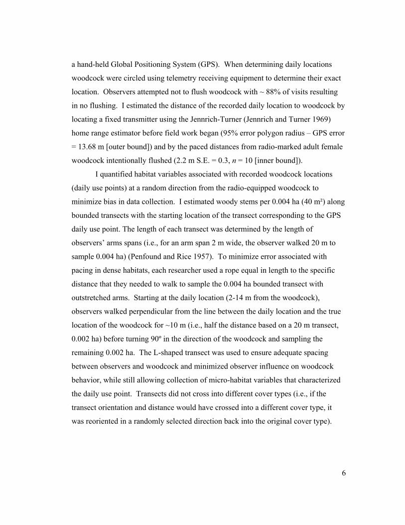
a hand-held Global Positioning System (GPS). When determining daily locations
woodcock were circled using telemetry receiving equipment to determine their exact
location. Observers attempted not to flush woodcock with ~ 88% of visits resulting
in no flushing. I estimated the distance of the recorded daily location to woodcock by
locating a fixed transmitter using the Jennrich-Turner (Jennrich and Turner 1969)
home range estimator before field work began (95% error polygon radius – GPS error
= 13.68 m [outer bound]) and by the paced distances from radio-marked adult female
woodcock intentionally flushed (2.2 m S.E. = 0.3, n = 10 [inner bound]).
I quantified habitat variables associated with recorded woodcock locations
(daily use points) at a random direction from the radio-equipped woodcock to
minimize bias in data collection. I estimated woody stems per 0.004 ha (40 m²) along
bounded transects with the starting location of the transect corresponding to the GPS
daily use point. The length of each transect was determined by the length of
observers’ arms spans (i.e., for an arm span 2 m wide, the observer walked 20 m to
sample 0.004 ha) (Penfound and Rice 1957). To minimize error associated with
pacing in dense habitats, each researcher used a rope equal in length to the specific
distance that they needed to walk to sample the 0.004 ha bounded transect with
outstretched arms. Starting at the daily location (2-14 m from the woodcock),
observers walked perpendicular from the line between the daily location and the true
location of the woodcock for ~10 m (i.e., half the distance based on a 20 m transect,
0.002 ha) before turning 90º in the direction of the woodcock and sampling the
remaining 0.002 ha. The L-shaped transect was used to ensure adequate spacing
between observers and woodcock and minimized observer influence on woodcock
behavior, while still allowing collection of micro-habitat variables that characterized
the daily use point. Transects did not cross into different cover types (i.e., if the
transect orientation and distance would have crossed into a different cover type, it
was reoriented in a randomly selected direction back into the original cover type).

7
Predictor variables
At woodcock use sites, observers measured stem density, estimated
earthworm abundance, assessed soil color, and collected soil samples. Observers
counted each vertical woody stem within the bounded transect that forked below
breast height as an individual stem and then tallied all stems counted within the
bounded transect to estimate the stem density in the habitat surrounding the
woodcock daily use point (Penfound and Rice 1957). Earthworm biomass was
measured within a 35 cm² (0.1225 m2) square plot at the daily use point. Any
vegetation inside this 35 cm² plot was cleared to facilitate detection and removal of
surfacing earthworms. Observers poured ~1.26 l (1/3 gallon) of oriental hot mustard
solution onto the ground, and collected all earthworms that surfaced during a 5
minute period (Paulson and Bowers 2002). In order to compare worm samples across
a large geographic area (Hale et al. 2004), I calculated ash-free dry mass for each
earthworm sample. Samples were weighed to the nearest 0.0001 g.
At the same location where earthworms were sampled, soil color was
quantified before pouring the hot mustard solution inside the plot. Soil color was
separated into 6 categories based on the Munsiel soil color chart 7.5YR (Munsiel
2000). The classifications used were 2.5-1, 3-1, 4-1, 5-1, 6-1, 8-1, and the closest
match to the soil color was recorded at the woodcock location. Approximately 1 m
from the earthworm sample location, observers collected a 9.8 cm diameter by 6.8 cm
deep (512.9 cm3) soil core at the surface. The soil sample was collected at a random
direction from the earthworm plot. When collecting soil samples, observers made
effort not to compact soils, so that bulk density was not artificially inflated (Blake and
Hartge 1986). I determined the porosity of the soil samples by dividing the bulk
density of the samples by the density of quartz (2.65 g/cm2) to find the amount of
pore space in the soil sample (Danielson and Sutherland 1986).
Daily weather variables were also collected in each of the 3 study locations.
Daily high and low temperatures in ºC were recorded with automated digital
thermometers located on or adjacent to study areas. Precipitation (cm) in the previous

8
24 hr period daily was recorded at 0900 with rain gauges located centrally at study
locations.
Movement data
Distance to subsequent locations (response variable) was calculated using the
animal movement extension (Hooge and Eichenlaub 1997) in Arcview 3.3
(Environmental Systems Research Institute 2002). Each individual woodcock
locational data set was structured by date and transformed into a polyline file. The
distance to the next subsequent point was automatically computed and stored for each
individual woodcock location. We did not monitor night-time locations of woodcock,
but the median distance from capture locations (roosting fields) to diurnal locations
was 414 m, which is similar to the distance between adult female woodcock roosting
sites and daytime foraging sites (179.5 m) observed in September and October in
Maine (Sepik and Derleth 1993).
A priori models
When woodcock return from their nighttime roosting fields a choice of diurnal
habitat and spatial use occurs. Therefore, I hypothesized a set of models prior to data
analysis based on the assumption that favorable environmental conditions on a
previous day would result in shorter distances between daily locations, because
woodcock would return to exploit favorable conditions. There are advantages to
returning to the same patch, such as familiarity with cover to avoid predators and
knowledge of productive foraging areas, but at some point surrounding habitats
would likely become more favorable when resources become depleted or when
availability of resources elsewhere was higher. In addition, weather events may
influence energy requirements.
I created 27 different models to evaluate the relationship between
environmental variables and movement of woodcock (Appendix 1). All predictor
variables were related to 3 major classes of models; food, weather, and predator
9
avoidance (Table 1). The distance between subsequent daily locations was the
response variable in all models. Inclusion of predictor variables was based on
published literature and my experience with woodcock movement in 2001, the pilot
year of my study.
Food models.-- Earthworms are the primary prey of woodcock. Earthworm
abundance likely varies both spatially and temporally and thus may influence
observed woodcock movement patterns. Earthworm abundance may be influenced
by several factors, including soil moisture (e.g., Sepik 1984, Straw et al. 1994), soil
temperature (<5 ºC or > 25 ºC; Reynolds et al. 1977, Rabe et al. 1983a), and
vegetation (Reynolds et al. 1977, Keppie and Whiting 1994). I hypothesized that an
increase in the mass of earthworms collected at a daily use point would be correlated
with a decrease in the distance to the subsequent daily location because I predicted
that woodcock should return to exploit high earthworm abundance. The second
variable relating to food resources was soil color. Soil colors that were darker were
hypothesized to result in shorter distances between daily locations based on
experimental evidence indicating that captive woodcock exhibited strong selection for
dark soil colors (Rabe et al. 1983b). The final variable included in the food models
was soil porosity. Porosity of the soil influences soil moisture, which likely
influences availability of earthworms (Rabe et al. 1983a, Sepik 1984, Straw et al.
1994) by influencing both abundance of earthworms and soil conditions that affect
foraging success by making it easier or harder for woodcock to find or extract
earthworms. I did not hypothesize a directional response related to porosity of the
soil, but suspected that there would be a threshold at which adequate moisture would
be present to support foraging for earthworms.
Weather models.-- Previous day’s precipitation was included in models
because I observed large movements following rain events in 2001 in Minnesota. I
included an interaction between rainfall and porosity of the soil in some models
because rainfall influences soil moisture. Highly porous soils that were previously
too dry for woodcock to forage successfully would likely become favorable after rain
events stimulating selection, thus movements into new areas. Cold temperatures may

10
also affect woodcock energetic requirements or foraging abilities (Bell 1991), which I
represented in models with daily low temperature. Woodcock metabolic demands
increase at lower temperatures (Haegen et al. 1994), but woodcock could respond to
increased metabolic demands by either increasing movement to increase foraging
opportunities or decreasing movements to conserve energy.
Predator avoidance models.-- By decreasing their exposure to predators
woodcock could decrease (1) handling time of prey, (2) observational vigilance for
predators, and (3) inter-prey waiting time (Krebs 1980), increasing their energetic
intake. Because I could not directly measure predation pressure, and because stem
densities at foraging locations were not correlated with earthworm abundance (food
models), I used stem density as a surrogate to predator avoidance. I hypothesized that
an increase in the density of the stand would offer woodcock increased protection
from predators (especially avian predators) and would decrease movement between
daily locations, because they could forage with less risk of predation.
Interactions.-- Due to the observational nature of my study I limited my
models to include only 3 first order interactions. First, I included the interaction
between rainfall and porosity of the soil discussed previously. Second, I allowed for
an interaction between earthworm abundance and low temperature because
earthworms become less available (<5 ºC or >25 ºC; Reynolds 1977, Rabe et al.
1983a) and this interaction was equally likely to stimulate or inhibit woodcock
movement. Third, I allowed for an interaction between soil color and rainfall,
because increased soil moisture (following rainfall) makes soil color darker.
Models were first created in each of the 3 main classes of variables with no
interactions included to determine whether individual or groups of variables were
strongly selected. In each suite of models, predictor variables were created alone
before they were combined with other variables. After creating each class of models
I combined variables from different classes of models. Finally, all 3 classes of
variables were combined. I had 2 global models that contained all parameters plus
first order interactions thought to be relevant to movement from field observations.
After I created all 27 models, they were then combined into a single candidate model

11
set and allowed to compete against each other. Only models having logical
mechanisms based on published literature or field observations were included in the
model set, therefore, all possible combinations of parameters were not included.
Data Analysis
Habitat variables collected at a woodcock locations were associated with the
distance that the woodcock moved to the subsequent location. In this manner the
distance that a bird moved between subsequent diurnal locations was a function of the
habitat that it occupied prior to moving. All adult female woodcock with >20
movements (n = 58) were included in the movement portion of the analysis. Because
sequential movements can be serially-correlated and habitat characteristics estimated
for the same woodcock closer in time are more likely to be correlated than measures
more distant in time, I modeled the appropriate covariance structure that best
represented the data in SAS PROC MIXED (Littell et al. 1996, 1998). The
covariance structure is derived from variances at individual times and correlations
between measures at different times on the same animal (Littell et al. 1998). Three
covariance structures were tested; compound symmetry (CS) where all measures at
all times have the same variance and all pairs of measures on the animal have the
same correlation, “unstructured” (UN) where no assumptions regarding equal
variances or correlations are made, and auto-regressive (ar1) where there is an inter-
animal random effect and a correlation structure within animals that decreases with an
increase in the time interval between measures (Littell et. al. 1996). SAS PROC
MIXED is a generalization of a standard linear model and data are permitted to
exhibit correlation and nonconstant variability (SAS 8.2 online doc.). I used the
REPEATED statement in PROC MIXED to model the covariation within woodcock,
which accounts for the violation of independence of the observations (Littell et al.
1998, Franklin et al. 2001). The RANDOM statement was used to model the
variation among woodcock, which accounts for heterogeneity of variances from
individual woodcock (Littell et al. 1998, Franklin et al. 2001). The random effects
factor was the sub-sample of individual woodcock that were randomly chosen from

12
all radio-marked adult female woodcock captured as part of the larger survival study.
All other factors in the model were fixed effects. Maximum likelihood methods were
then used to fit a mixed-effects (both random and fixed effects) general linear model
in SAS PROC MIXED. I used Akaike’s Information Criterion (AICc) to rank
competing models based on which models were best supported by the observed data
(Akaike 1973, Burnham and Anderson 2002). AICc values computed in PROC
MIXED were used to identify the model with the highest rank (i.e., minimum AICc
value) and ∆AICc values were used to calculate the likelihood of the model given the
data using the following equation from Burnham and Anderson (2002:74).
ℓ(gi│x) α exp(- ½∆i) (1)
ℓ(gi│x) = the likelihood(ℓ) of the model( gi) given the data(x).
“α” means “is proportional to”
and ∆i is the AIC differences (AIC(gi) – AIC(minimum value))
Likelihood estimates from equation 1 where used to calculate Akaike weights
using equation 2 (Burnham and Anderson 2002:75),
exp(- ½∆i) . wi = R (2) ∑ exp(- ½∆r)
r =1
which can be interpreted as the “weight of evidence in favor of model i being the
actual Kullback-Leibler (K-L) best model for the situation at hand given that one of
the R models must be the K-L best model of that set of models” (Burnham and
Anderson 2002:75).
To assess how much variation among individual woodcock was explained by
the best approximating models I conducted a variance-components analysis (Littell et
al. 1996, Franklin et al. 2001). I used maximum likelihood covariance parameter
13
estimates from SAS PROC MIXED for the ∆AICc best models and the “means
model” (constant only) to compute the amount of process variation explained:
process variation explained = (ơ(,)-ơ a) / ơ(,) (3)
where ơ(,) = the variance component estimate for constant only model
and ơ a = the variance component estimate for the a priori model
To test whether pooling data across 3 study areas was justified, the suite of
models (n = 27) was calculated with study area and year as blocking factors, and I
assessed whether model selection or Akaike weights changed. Although most
movements between subsequent locations were short (~ 95% of movements <500 m)
woodcock also made longer movements up to 3,806 m. To test the sensitivity of the
relative importance of each model and the amount of process variation explained by
the effects of these large movements (>500 m), the same analysis that was performed
on the full data set was performed on a subset of the data that incorporated only
movements that were <500 m. Results from this analysis were then compared to
analyses of the full data set. I used the best approximating model to estimate and
compare regression coefficients and standard errors.
Results:
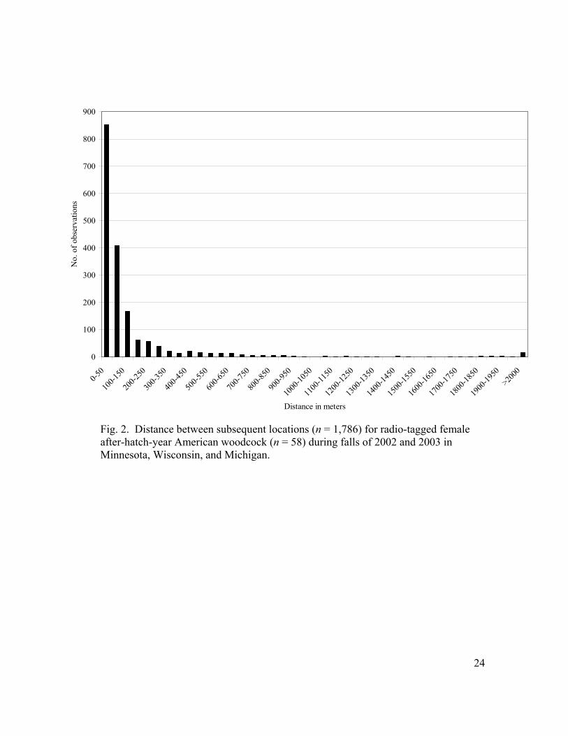
The majority (90.9%) of distances between subsequent daily locations by
woodcock were <400 m, with 47.7% of the movements being <50 m (Fig. 2). The
distance between subsequent daily locations for adult female American woodcock
where generally small with the median distance being 52.0 m, but were highly
variable (C.V. = 2.9, Table 2). Mean ash-free dry earthworm mass was 0.077 g (S.D.
0.153, C.V. = 1.99). Woodcock were located in areas having porous soils with mean
porosity of soil samples being 0.774 (S.D. = 0.096, C.V. = .13) and in dense stands
with an average of 114.18 stems per 0.004 ha (S.D. = 76.06, C.V. = 0.66).
The combined effects of low temperatures, precipitation, earthworm biomass,
porosity of the soil, and a rain*porosity interaction were the strongest predictors of

14
woodcock movements. Of the 27 models tested, 2 models, which were identical
except for the inclusion of the rain*porosity interaction (T+R+W+P+R*P [model 1]
and T+R+W+P [model 2]), had a strong combined weight of evidence (wi = 0.914)
that they were the best models in the analyses of the full data set (Table 3). Food and
weather were the best predictors of movements. The inclusion of the rain*porosity
interaction greatly increased the likelihood that model 1 was the best predictor of
woodcock movements with an evidence ratio of 5.48 when compared to model 2.
The covariate structure selected based on Information-theoretic methods was ar(1),
which I used in all mixed modeling.
An increase in earthworm mass was negatively correlated with the distance
moved to subsequent locations and an increase in temperature was positively
correlated with the distance moved to subsequent locations (Table 4). Earthworm
mass had a large standard error compared to its associated parameter estimates. The
effects of rain was negatively correlated with movements when the rain*porosity
interaction was included (model 1). An increase in porosity was associated with an
increase in distance between subsequent locations. The rain*porosity interaction had
the strongest positive effect on the movements of adult female woodcock.
The inclusion of study areas and year as blocking factors did not affect the
relative importance of the models evaluated or substantially change Akaike weights
(Table 3). The inclusion of study area and years, however, increased the amount of
variation explained by environmental factors among individual woodcock movements
from 21.39 to 71.56%.
The same 5 models were selected from 27 a priori models for movements
<500 m as for all movements, however the relative importance of the top 2 models
switched, decreasing the importance of the interaction between rainfall and porosity
(model 1 wi = 0.277, model 2 wi = 0.716 [Table 5]). The same combined effects of
low temperatures, precipitation, earthworm biomass, soil porosity, and a
rain*porosity interaction were the strongest predictors of woodcock movements <500
m. The top 2 models combined (T+R+W+P+ R*P and T+R+W+P) had a strong
combined weight of evidence (wi = 0.993) that they were the best models of
15
movements <500 m (Table 5). Model 2 had an evidence ratio of 2.585 vs. model 1
(with interaction). In contrast to the high amount of variation explained among
individual woodcock by the best model in the analysis of all movements (71.56%
with years and study areas as blocks), the best model for movements <500 m
explained very little of the variation among woodcock (3.86%, with years and study
areas as blocks). For the best model, S.E. estimates for all parameters were larger
than the associated regression coefficient estimate except for T (regression estimate
0.675, S.E. = 0.277), which still had a positive effect on movement.
Discussion:
The distance between subsequent fall daily locations for adult female
American woodcock in Minnesota, Wisconsin, and Michigan were generally small
(median distance = 52.0 m), indicating that woodcock returned to the vicinity of the
previous day’s foraging area. Of the 27 a priori models I constructed, hypothesized
to relate to food, weather, and predator avoidance, the same 5 models related to food
and weather were selected, regardless of study site (3 states), replication (2 years), or
the distance of movements considered (all movements, or movements <500 m).
In contrast to the high amount of variation explained among individual
woodcock for all movements (71.56%), the best models explained only ~ 3.8% of the
process variation among birds for movements <500 m. There are several plausible
explanations for differences in predictive power at different scales of movements.
First, the effect size could be too small in relation to the high variability in
movements <500 m (C.V. = 2.2) to effectively predict movements. Second, predictor
variables also exhibited high variability, thus creating large standard errors for
parameter estimates. Third, if woodcock were selecting habitat on different scales for
shorter vs. farther movements, and movements <500 m were based on features that
varied at a small spatial scale (i.e., smaller than the distance between the woodcock
and where we sampled habitat variables), then our study design would have low
power to detect these effects. The distance that we kept from woodcock in order to
minimize impacts on behavior could have led to the quantification of habitat at the

16
patch level instead of the micro-habitat characteristics of the use point, reflected in
the high predictive power of models of movements when woodcock changed patches.
Finally, variables that were quantified may not represent factors affecting shorter
movements of adult female woodcock.
When all movement data were included in analyses, my models explained a
high proportion (71.56%) of the process variation among woodcock and model
parameter estimates coincided with my a priori hypotheses about adult female
woodcock movements. Parameter estimates from the best approximating models and
scatter plots (Appendix 2) indicated that increasing earthworm biomass was related to
decreased movement distances. From the stand point of optimal foraging,
specifically the marginal value theorem (MacArthur and Pranka 1966, Charnov
1976), it is likely that the woodcock returned to forage in areas with high earthworm
mass until conditions become more favorable in other areas. Woodcock were more
likely to make large movements (>500 m) and forage in new areas when earthworm
mass at the previous day’s foraging site was low.
Other constraints such as predator avoidance may also influence habitat
selection, but stand density was not a strong predictor of movement distance in my
analyses at any scale of movement. I used stem density as a surrogate of predator
avoidance and other factors related to predator avoidance that were not measured
could also influence woodcock habitat selection, such as the effectiveness of their
cryptic plumage against different backgrounds. While soil color was strongly
selected in feeding trials of American woodcock (Rabe et al. 1983a), my results did
not indicate that woodcock movement was related to soil color.
Decreasing daily low temperature was negatively correlated with movement
distances, with >2/3 of movements >500 m occurring when the daily low temperature
was above the median low temperature of 2.4 ºC (Appendix 3). This suggests that
woodcock make fewer large movements to conserve energy when decreasing
temperatures increase metabolic demands. Conservation of energy has been
documented during a drought in Maine, where woodcock ceased to make flights to
nocturnal roosting areas in conditions of low food availability (Sepik et al. 1983).

17
Results of laboratory studies of bumble bee and dark-eyed junco (Junco hyemalis)
foraging (Cartar and Dill 1990, Caraco et al. 1990) suggested that animals may
minimize unpredictability and prefer less risky foraging opportunities even if risky
foraging is more profitable. However, when dark-eyed juncos were exposed to stress
from decreasing low temperatures their response was to adopt a more risky foraging
behavior. My results suggest that woodcock do not exhibit the same response to
decreasing temperatures, perhaps because when soil temperatures are below 5 ºC
earthworms become less active (Reynolds et al. 1977, Rabe et al. 1983a), and
presumably less available to woodcock.
Soil porosity had a positive relationship to the distance moved between
subsequent daily locations; approximately 2/3 of movements >500 m occurred when
porosity values were greater than the median porosity value of 0.770 (Appendix 4).
The positive relationship of soil porosity was linked to the interaction between rain
and porosity, suggesting woodcock responded to this interaction by making large
movements into new foraging areas that were previously too dry to adequately
provide them with their primary food source, earthworms. The combination of rain
and porosity interacting together exhibited the greatest positive relationship to
movement than any of the predictive variables. The positive relationship of porosity
on movements was decreased by more than 50% in model 2 compared to when the
interaction between R*P was included in model 1. The importance of the rain and
porosity interaction to movements >500 m is further supported by the fact that the
relative importance of model 1 (with the R*P interaction term) was greatly decreased
when movements >500 m were not included in analyses (wi = 0.277). Finally, this
was consistent with field observations where woodcock made large movements into
previously unused areas after precipitation events.
My interpretation of the way woodcock move and where they choose to be
from day to day is that unless some environment stimuli occurs making conditions
more favorable elsewhere, adult female woodcock will return to the previous day’s
foraging area. In this study, woodcock were more likely to make large movements
(>500 m) and risk foraging in new areas when environmental conditions were not

18
favorable, such as in the case of low earthworm biomass, or when metabolic demands
decreased at higher temperatures. The strong influence of the interaction of soil
porosity and rain also suggests that habitat use is influenced by prevailing conditions
that affect habitat quality at a particular time. Assessing movement behavior in
woodcock allowed insight into why birds moved and how they used habitat,
providing assessment of habitat selection beyond determination of preference alone.
Adult female woodcock appeared to incorporate prior knowledge of previously used
areas into the decision of where they will forage on a particular day.
Literature cited:
Akaike, H. 1973. Information theory as an extension of the maximum likelihood
principle. Pages 267-281 in B.N. Petrov and F. Csaki, eds. Second International Symposium on Information Theory. Budapest, Akademiai Kiado.
Bell, W.J. 1991. Searching behavior: the behavioral ecology of finding resources.
Chapman and Hall. New York, New York, USA.
Burnham, K.P. and D.R. Anderson. 2002. Model selection and multimodel inference. Springer-Verlag, New York, New York, USA.
Blake, R.E. and K.H. Hartge. 1986. Bulk density. Pages 363-375 in A. Klute, ed. Soil Science Society of America Handbook Series 5. Soil Society of America, Madison, Wisconsin, USA.
Caraco, T., W.U. Backenhorn, G.M. Gregory, J.A. Newman, G.M.Recer, and S.M. Zwicker. 1990. Risk-sensitivity: ambient temperature affects foraging choice. Animal Behavior 39:338-345.
Cartar, R.V. and L.M. Dill. 1990. Why are bumblebees risk-sensitive foragers?
Behavior Ecology and Sociobiology 26:121-127. Charnov, E.L. 1976. Optimal foraging: the marginal value theorem. Theoretical
Population Biology 9:129-136.
Danielson, R.E. and P.L. Sutherland. 1986. Porosity. Pages 443-445 in A. Klute, ed. Soil Science Society of America Handbook Series 5. Soil Society of America, Madison, Wisconsin, USA.
19
Environmental System Research Institute. 2002. 380 New York Street, Redlands, CA 92373-8100.
Godfry, G.A. 1974. Behavior and ecology of American woodcock on the breeding range in Minnesota. Dissertation, University of Minnesota, Minneapolis, Minnesota, USA.
Franklin, A.B., T.M. Shenk, D.R. Anderson, and K.P. Burnham. 2001. Statistical model selection; an alternative to null hypothesis testing. Pages 75-90 in T.M. Shenk and A.B. Franklin eds. Modeling in natural resource management. Island Press Washington D.C. USA.
Haegen,W.M., R.B. Owen Jr., and W.B. Krohn. 1994. Metabolic rate of American woodcock. Wilson Bulletin 106:338-343.
Hale, C. M., L. E. Frelich, and P. B. Reich. 2004. Allometric equations for estimation of ash-free dry mass from length measurements for selected European earthworm species (Lumbricidae) in the western Great Lakes region. American Midland Naturalist 151:179-185.
Heller, R. and M. Milinski. 1979. Optimal foraging of sticklebacks of swarming
prey. Animal Behavior 27:1127-1141.
Hooge, P.E. and B. Eichenlaub. 1997. Animal movement extension to Arcview: Version 2.0. Alaska Biological Science Center, U.S. Geological Survey, Anchorage, Alaska, USA.
Hudgins, J.E., G.L. Storm, and J.S. Wakely. 1985. Local movements and diurnal-habitat selection of male American woodcock in Pennsylvania. Journal of Wildlife Management 49:614-619.
Jennrich, R.I. and F. B. Turner. 1969. Measurement of non-circular home range. Journal of Theoretical Biology 22:227-237.
Keppie, D.M. and R.M. Whiting, Jr. 1994. American woodcock Scolopax minor. The Birds of North America. 100:1-27. American Ornithologists’ Union and Academy of Natural Sciences of Philadelphia, USA.
Krebs, J.R. 1980. Optimal foraging, predation risk and territory defense. Ardea
80:83-90.

20
---------- and N.B. Davies. 1993. An introduction to behavioral ecology. Blackwell Science Ltd. Malden, Massachusetts, USA
Krohn, W.B. 1971. Some patterns of woodcock activities on Maine summer fields.
Wilson Bulletin. 83: 396-407 Lima, S., T.J. Valone, and T. Caraco. 1985. Foraging efficiency-predation risk
tradeoff in the grey squirrel. Animal Behavior 33:155-165.
Littell, R.C., G.A. Milliken, W.W. Stroup, and R.D. Wolfinger. 1996. SAS System for Mixed Models. SAS Institute, Cary, North Carolina, USA.
----------, P.R. Henry, and C.B. Ammerman. 1998. Statistical analysis of repeated measures data using SAS procedures. Journal of Animal Science 76:1216-1231.
Martin, F.W. 1964. Woodcock age and sex determination from wings. Journal of Wildlife Management 28:287-293.
MacArthur, R.H. and E.R. Pranka. 1966. On optimal use of a patch environment. American Naturalist 100:603-609.
McAuley, D. G., J.R. Longcore, and G.F. Sepik. 1993. Techniques for research into woodcocks: experiences and recommendations. Pages 5-11 in J.R. Longcore and G.F. Sepik, eds. Proceedings of the eighth woodcock symposium. Biological Report 16, U.S. Fish Wildlife Service, Washington D.C., USA.
Mendal, H.L. and C.M. Aldous. 1943. The ecology and management of the American woodcock. Maine Cooperative Wildlife Research Unit, University of Maine, Orono. Maine USA.
Milinski, M. and R. Heller. 1978. Influence of a predator on the optimal foraging behavior of sticklebacks (Gaserosteus aculeatus). Nature 275:642-644.
Morgenweck, R.O. 1977. Diurnal high use areas of hatching-year female American woodcock. Pages 155-160 in D.M. Keppie and R.B. Owen, Jr. eds. Proceedings of the sixth woodcock symposium. New Brunswick Department of Natural Resources, Fredericton, New Brunswick, Canada.
Munsell® Color. 2000. Munsell Soil Color Charts. GretagMacbeth, New Windsor, New York.
Paulson, L.A. and M.A. Bowers. 2002. A test of the `hot' mustard extraction method of sampling earthworms. Soil Biology and Biochemistry 34:549-552.
21
Penfound, W.T. and E.L. Rice. 1957. An evaluation of the arms length rectangle method in forest sampling. Ecology 38:660-661.
Pyke, G.H. 1983. Animal movements: an optimal foraging approach. Pages 7-31 in I.R. Swingland and P.J. Greenwood, eds The ecology of animal movement.
Clarendon Press, Oxford, UK.
Rabe, D.L., H.H. Prince, and E.D. Goodman. 1983a. The effects of weather on the bioenergetics of breeding American woodcock. Journal of Wildlife Management 47:762-771.
-------------, -------------, and D.L. Beaver. 1983b. Feeding-site selection and foraging strategies of American woodcock. Auk 100:711-716.
Reifenberger, J.C. and R.C. Kletzy. 1967. Woodcock nightlighting techniques and equipment. Pp 33-35 in W.H. Goudy, compiler. Woodcock research and management, 1966. U.S. Bureau of Sport Fisheries and Wildlife, Special Scientific Report- wildlife 101. 40pp.
Reynolds, J.W., W.B Krohn, and G.A. Jordan. 1977. Earthworm populations as related to woodcock habitat usage in central Maine. Pages 135-146 in D.M. Keppie and R.B. Owen Jr., eds. Proceedings of the sixth woodcock symposium. New Brunswick Department of Natural Resources, Fredericton, New Brunswick, Canada.
SAS online documentation version 8.2. SAS publishing, SAS Institute Inc. Cary, North Carolina, USA.
Sepik, G.F. 1984. Population ecology of woodcock in Wisconsin. Wisconsin Department of Natural Resources. Technical Bulletin 144. Pages 1-51.
---------- and E.L. Derelth. 1993. Habitat use, home range size, and patterns of moves of the American woodcock in Maine. Pages 41-49 in J.R. Longcore and G.F. Sepik, eds. Proceedings of the eighth woodcock symposium. Biological Report 16, U.S. Fish Wildlife Service, Washington D.C. USA.
----------, R.B. Owen, and T.J. Dwyer. 1983. The effects of a drought on a local woodcock population. Transactions of the Northeast Section of The Wildlife Society 40:1-8.
Sheldon, W.G. 1960. A method of mist netting woodcock in summer. Bird-banding 31:130-135.

22
Straw, J.A. Jr., D.G. Krementz, M.W. Olinde, G.F. Sepik. 1994. American Woodcock. Pages 97-114 in T. Tacha and C. Braun, eds. Migratory, shore, and upland gamebird management in North America. International Association of Fish and Wildlife Agencies.
Whitcomb, D.A. 1974. Characteristics of an insular woodcock population. Michigan Department of Natural Resources Wildlife Division Report 2720.
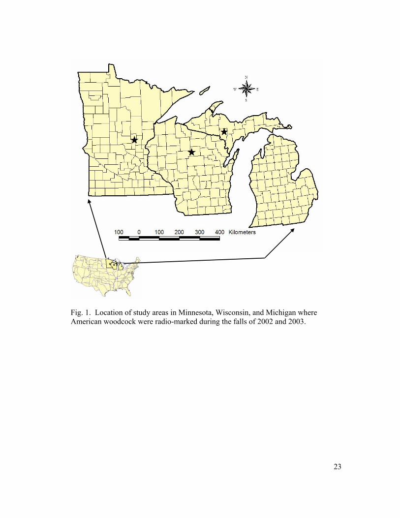
Fig. 1. Location of study areas in Minnesota, Wisconsin, and Michigan where American woodcock were radio-marked during the falls of 2002 and 2003.
23
0
100
200
300
400
500
600
700
800
900
0-50
100-1
50
200-2
50
300-3
50
400-4
50
500-5
50
600-6
50
700-7
50
800-8
50
900-9
50
1000
-1050
1100
-1150
1200
-1250
1300
-1350
1400
-1450
1500
-1550
1600
-1650
1700
-1750
1800
-1850
1900
-1950
>2000
Distance in meters
No.
of o
bser
vatio
ns
Fig. 2. Distance between subsequent locations (n = 1,786) for radio-tagged female after-hatch-year American woodcock (n = 58) during falls of 2002 and 2003 in Minnesota, Wisconsin, and Michigan.
24

25
Table 1. American woodcock movement predictor variables and covariates at locations determined via radio telemetry in 2002 and 2003, in central Minnesota, central Wisconsin, and the Upper Peninsula of Michigan. Parameter Symbol Model Class Daily low temperature (ºC) T Weather Daily precipitation (cm) R Weather Soil color C Food Ash-free earthworm dry mass
W Food
Porosity of soil P Food No. stems per 0.004 ha S predator avoidance

26
Table 2. Descriptive statistics of predictor variables and distances between subsequent locations (n = 1,786) of after-hatch-year female American woodcock (n = 58) in central Minnesota, central Wisconsin, and the Upper Peninsula of Michigan during the falls of 2002 and 2003.
Low Temp (ºC)
Precipitation (cm)
Ash-free dry mass
(g) Porosity of
soil (%) Stems per 0.004 ha
Distance (m)
Minimum -9.3 0.00 0.000 0.47 0.0 0.6Maximum 17.5 21.30 1.915 1.00 457.0 3806.7Median 2.4 0.00 0.020 0.77 100.0 52.0Mean 3.2 0.48 0.077 0.77 114.9 156.6Std. Error 0.1 0.04 0.004 0.01 1.8 8.1Std. Dev. 5.9 1.78 0.153 0.10 76.1 342.6C.V. 1.8 3.73 1.994 0.13 0.7 2.9

27
Table 3. Effects of blocking on process variation explained and summary of best models (n = 5 of 27 a priori models) and means model predicting distances between subsequent daily locations of after-hatch-year female American woodcock (n = 58) in central Minnesota, central Wisconsin, and the Upper Peninsula of Michigan during the falls of 2002 and 2003.
Blocking Modela k AICC ∆AICCĹ (gi │x) wi ơb
(ơ(,)-ơa)/ ơ(,)
area,year T,R,W,P,R*P 8 18638.6 0 1.000 0.773 1321.550 71.561areas,year T,R,W,P 7 18642.0 3.4 0.183 0.141 1437.850 69.058areas,year T,R,C,W,P,T*W,R*P 10 18643.0 4.4 0.111 0.086 1347.130 71.010areas,year W,P 5 19423.1 784.5 0.000 0.000 2229.590 52.020areas,year P 4 20419.5 1780.9 0.000 0.000 3008.490 35.258
none (,) means model 1 4646.910 0.000
areas T,R,W,P,R*P 7 18637.2 0 1.000 0.774 3369.250 27.495areas T,R,W,P 6 18640.5 3.3 0.192 0.149 3456.130 25.625areas T,R,C,W,P,T*W,R*P 9 18641.8 4.6 0.100 0.078 1802.910 61.202areas W,P 4 19422.4 785.2 0.000 0.000 3735.420 19.615areas P 3 20418.2 1781 0.000 0.000 4164.280 10.386none (,) 1 4646.910 0.000
none T,R,W,P,R*P 6 18634.2 0 1.000 0.753 3652.770 21.394none T,R,W,P 5 18637.0 2.8 0.247 0.186 3717.870 19.993none T,R,C,W,P,T*W,R*P 8 18639.2 5 0.082 0.062 2236.850 51.864none W,P 3 19419.1 784.9 0.000 0.000 3936.600 15.286none P 2 20414.6 1780.4 0.000 0.000 4315.970 7.122 none (,) 1 4646.910 0.000
a W = worms, P = porosity, T = low temp, R = rain in cm3 , (,) = constant only b
ơ = covariance parameter estimate
28
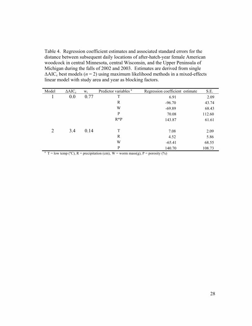
Table 4. Regression coefficient estimates and associated standard errors for the distance between subsequent daily locations of after-hatch-year female American woodcock in central Minnesota, central Wisconsin, and the Upper Peninsula of Michigan during the falls of 2002 and 2003. Estimates are derived from single ∆AICc best models (n = 2) using maximum likelihood methods in a mixed-effects linear model with study area and year as blocking factors. Model ∆AICc wi Predictor variables a Regression coefficient estimate S.E.
1 0.0 0.77 T 6.91 2.09 R -96.70 43.74 W -69.89 68.43 P 70.08 112.60 R*P 143.87 61.61 2 3.4 0.14 T 7.08 2.09 R 4.52 5.86 W -65.41 68.55 P 140.70 108.73
a T = low temp (ºC), R = precipitation (cm), W = worm mass(g), P = porosity (%)
29
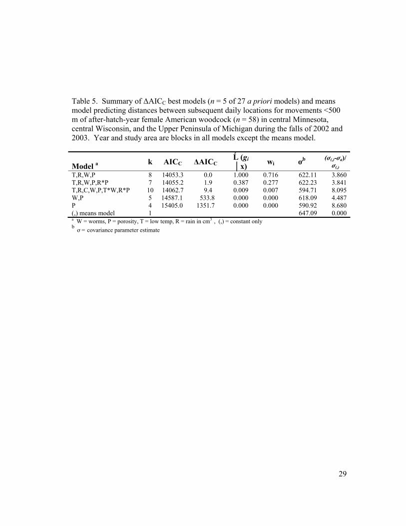
Table 5. Summary of ∆AICC best models (n = 5 of 27 a priori models) and means model predicting distances between subsequent daily locations for movements <500 m of after-hatch-year female American woodcock (n = 58) in central Minnesota, central Wisconsin, and the Upper Peninsula of Michigan during the falls of 2002 and 2003. Year and study area are blocks in all models except the means model.
Model a k AICC ∆AICC Ĺ (gi │x) wi ơb (ơ(,)-ơa)/
ơ(,) T,R,W,P 8 14053.3 0.0 1.000 0.716 622.11 3.860 T,R,W,P,R*P 7 14055.2 1.9 0.387 0.277 622.23 3.841 T,R,C,W,P,T*W,R*P 10 14062.7 9.4 0.009 0.007 594.71 8.095 W,P 5 14587.1 533.8 0.000 0.000 618.09 4.487 P 4 15405.0 1351.7 0.000 0.000 590.92 8.680 (,) means model 1 647.09 0.000 a W = worms, P = porosity, T = low temp, R = rain in cm3 , (,) = constant only b
ơ = covariance parameter estimate

30
Appendix 1. Summary of all a priori models (n = 27) used to evaluate the distance to subsequent daily locations (n =1,786) of after-hatch-year female American woodcock (n = 58) in central Minnesota, central Wisconsin, and the Upper Peninsula of Michigan during the falls of 2002 and 2003. Models in the final analysis included a blocking effect for study areas and years.
Model Class Parameters a k ∆AICC Weather T 2 5855.4 Weather R 2 5660.3 Weather T,R 3 5604.5 Food C 2 6696.6 Food W 2 5411.3 Food P 2 1780.9 Food W,C 3 5413.3 Food W,P 3 784.5 Predation S 2 6616.8 Weather + Food T,R,W,C 5 4375.8 Weather + Food T,R,W,P 5 3.4 Weather + Food + Interaction T,R,W,C,T*W,R*C 7 4380.1 Weather + Food + Interaction T,R,W,P,R*P 6 0.0 Interaction T*W, R*C 3 4396.9 Weather + Predation T,R,S 4 5524.7 Weather + Predation T,S 3 5580.9 Weather + Predation R,S 3 6617.1 Predation + Food S,C 3 5345.3 Predation + Food W,S 3 5347.5 Predation + Food W,S,C 4 4308.9 Weather + Predation + Food T,R,W,S,C 6 4306.8 Weather + Predation + Food T,P,W,S 5 4368.7 Weather + Predation + Food R,W,S,C 5 4559.3 Weather + Predation + Food T,W,S 4 4559.3 Weather + Predation + Food R,W,S 4 4366.4 Global T,R,C,W,P,T*W,R*P 8 4.4 Global T,R,C,W,S,T*W 7 4310.9 a T = daily low temp, R = rain in cm , C = soil color, W = worms, P = porosity, S = stems per 0.004 ha

Appendix 2. Plot of the ash-free dry weight of earthworm samples (g) vs. the distance traveled to subsequent daily locations (n = 1,786) for after-hatch-year female American woodcock (n = 58) in central Minnesota, central Wisconsin, and the Upper peninsula of Michigan during the falls of 2002 and 2003.
2.0
31
1.5
1.0
0.5
0.0
Ash
-Fre
e D
ry W
eigh
t (g)
0 1000 2000 3000 4000
Distance(m)

Appendix. 3. Plot of low temperature in ºC vs. the distance traveled to subsequent daily locations (n = 1,786) for after-hatch-year female American woodcock (n = 58) in central Minnesota, central Wisconsin, and the Upper Peninsula of Michigan during the falls of 2002 and 2003.
20
32
10
0
-10
Low
Tem
pera
ture
(ºC
)
0 1000 2000 3000 4000
Distance (m)

Appendix 4. Plot of the percent porosity of soil samples vs. the distance traveled to subsequent daily locations (n = 1,786) for after-hatch-year female American woodcock (n = 58) in central Minnesota, central Wisconsin, and the Upper Peninsula of Michigan during the fall of 2002 and 2003.
0 1000 2000 3000 4000
Distance (m)
0.4
0.5
0.6
0.7
0.8
0.9
1.0
Poro
sity
of s
oil (
%)
33

34
Chapter 2
Fixed kernel home range estimation incorporating telemetry
location error: American woodcock (Scolopax minor) home
range analysis using real and simulated data
Abstract:
Bandwidth selection in fixed kernel home range estimation can influence
interpretation of results, especially when data are over-smoothed. Currently, the
accepted method of bandwidth selection is least square cross validation, which
results in unbiased use area estimates, but may also result in large areas of unused
habitat being included. An alternative to least squares cross validation may be
using error associated with telemetry locations, which represents the resolution at
which data are collected. To evaluate using telemetry error in fixed kernel home
range estimation, I analyzed American woodcock (Scolopax minor) home ranges
derived from telemetry data using fixed kernels with two different bandwidth
selection methods coupled with bootstrap re-sampling and Monte Carlo
simulations. The method of using 95% circular error probability from data points
as the smoothing parameter (her ) was compared to least squares cross validation
(hlscv ) as an automated bandwidth selection method. I tested each bandwidth
selection method’s sensitivity to sample size, non-continuous use of space, and
impacts of outliers to the 95% and 50% probability areas. Using hlscv resulted in a
low coefficient of variation (C.V. ~ 0.11) and comparable area estimates at low
sample sizes (n > 30) if the home ranges were continuous, had no outliers, and
had a single core area. In simulations with a sample size of 50, the presence of 1
outlier area with 2 locations, or having 2 core areas separated in space
significantly biased probability areas upward when using hlscv as the smoothing

35
method in a fixed kernel. Using her resulted in a low C.V.( ~ 0.11) and
comparable area estimates for the 95% probability areas at low sample sizes (n >
30), regardless of the presence of outliers or non-continuous spatial use. Home
range estimates using her were consistent with published home range estimates for
after-hatch-year female woodcock during the fall, and outperformed hlscv at
moderate sample sizes (n = 30-50) in Monte Carlo simulations. I conclude that her
is a viable alternative to hlscv as an automated, non-arbitrary, selection of
bandwidth, especially in cases with modest sample sizes, outliers, or non-
continuous spatial use. Using her as the smoothing parameter for fixed kernel
estimation represented the finest resolution (smoothing) home range estimate
supported by field data.
Introduction:
Since the inception of the concept of home range (Burt 1943), there have
been many methods proposed to quantify the area in which an animal moves during
its normal activities. These include non-statistical models such as the minimum
convex polygon (MCP [Mohr 1947]), bivariate normal statistical models (Jennrich
and Turner 1969), grid methods such as harmonic mean (Dixon and Chapman 1980),
and a non-parametric probabilistic kernel estimator (Worton 1989). Kernel
estimation has long been used in the field of statistics (Silverman 1986) and the fixed
kernel is now widely regarded as the preferred method for home range estimation in
the ecological literature (e.g., Seaman and Powell 1996, Kernohan et al. 2001).
Kernels are distribution free, free of assumptions except independence among
data points (Silverman 1986), and have performed well in simulation studies (Worton
1995, Seaman and Powell 1996, Seaman et al. 1999). However, the choice of a
smoothing parameter is widely regarded as the most important factor in the
performance of kernel estimation (e.g., Silverman 1986, Worton 1995, Kernohan et
al. 2001). Insufficient smoothing results in density estimates that are too rough and
contain spurious features that are artifacts of the sampling process, while over
smoothing results in loss of important features (Jones et al. 1996). Using least-
36
squares cross validation (hlscv) (Silverman 1986) in a fixed kernel is widely used as
the default bandwidth choice for smoothing and is the current recommendation in the
ecological literature (Seaman and Powell 1996).
Unfortunately, there is a large bias vs. variance trade off in the selection of
bandwidth in the use of kernels (Silverman 1986) with hlscv being an extreme case
resulting in non-biased estimates with high variability (Jones et al. 1996, Park and
Marron 1990, Hansten et al. 1997). Kernels have also been shown to overestimate
the 95% probability area in simulation studies and Worton (1995) applied correction
factors to hlscv to control for this overestimation. Kernels do not have a variance and
therefore do not permit sample size calculations in experimental design or measures
of precision of estimated areas (White and Garrott 1990). Seaman et al. (1999)
performed a simulation study to address this issue and recommended a minimum of
30 points, with 95% probability areas generally reaching an asymptote at around 50
points. To date however, there are no studies that address sample size issues using
real field data coupled with bootstrap re-sampling and Monte Carlo simulations.
Herein, I use telemetry data from American woodcock (Scolopax minor) to assess
kernel estimation of home range size.
American woodcock make crepuscular flights from nighttime roosting fields
to densely wooded diurnal areas with moist soils. Distance between observed
subsequent daily locations in past studies are relatively far (129 m [Sepik and Derleth
1993], 122.81 m ± 12.81 SE [Andersen et al. 2003]) compared to movements within
the same day (median distance ~5 m [Hudgins et al. 1985], average 22.0 m ± 1.7 SE
[Godfrey 1974]). Unless woodcock are disturbed, they generally remain in the same
small patch of habitat all day (D. G. McAuley, U.S. Geological Survey, personal
communication and field observations). Woodcock are generally located in the same
stand each day, but some woodcock have >1 area of concentrated use separated by a
substantial distance by areas of non-use. Because the smoothing parameter in hlscv is
estimated from the distance to all points from each particular grid intersection, large
distance between use areas leads to oversmoothing. In our study, many woodcock

37
also made large pre-migratory movements before returning to their core area and
subsequently migrating for the winter (Andersen et al. 2003). These long-distance
movements also could bias the smoothing parameter derived using hlscv leading to an
oversmoothed home range estimate that yields little biologically useful information.
Other wildlife researchers have recognized this problem in the past and Naef-Daenzer
(1993) modified the kernel function so that it only calculated densities for points
below 1 SD from the grid intersection.
To assess estimation of woodcock diurnal home ranges from daily locations
during the fall, I (1) estimated sample size effects on the performance of fixed kernel
estimation on a real data set using bootstrap re-sampling, (2) assessed the effects of
non-continuous spatial use on kernel home range estimation, and (3) compared the
use of 95% circular area probability (precision of my daily location points as the
smoothing factor [her]) vs. hlscv in a fixed kernel. I conducted a simulation study in
Arcview 3.3 (Environmental Systems Research Institute 2002) with the animal
movements extension (Hooge and Eichenlaub 1997) to facilitate a direct comparison
with known home range areas exhibiting the same patterns as our radio-marked
sample of woodcock.
Study Area:
Woodcock telemetry data were collected on parts of the 15,672 ha
Mille Lacs Wildlife Management Area (MLWMA) and the adjacent 1,166 ha Four
Brooks Wildlife Management Area (FBWMA) in east-central Minnesota. Both
WMAs are managed to provide hunting opportunities to the public, primarily by
habitat manipulation for game species. Upland bird hunting (including hunting for
woodcock) was allowed on MLWMA, and the recently acquired FBWMA was closed
to woodcock hunting (not other game bird hunting) during the three-year study period
2001-2003. Data used in this analysis are from the 2003 field season. MLWMA is in
close geographic proximity to FBWMA and they have comparable vegetative
communities, which include early regenerating aspen (Populus spp.) and lowland

38
habitats including alder (Alnus spp.), willow (Salix spp.), and burr oak (Quercus
macrocarpa).
Methods:
Capture and radio-marking
I began capturing woodcock on 20 August 2003 in both the MLWMA and the
adjacent FBWMA. Woodcock were captured at night-roosting fields by means of
mist netting (Sheldon 1960) and by spot lighting roosting fields (Reifenburg and
Kletzy 1967, McAuley et al. 1993). Wing plumage characteristics were used to age
and sex captured birds (Martin 1964) and we used bill length as an additional means
of determining sex (Mendal and Aldous 1943). Captured woodcock were radio
marked using all-weather livestock tag cement in conjunction with a single-loop wire
harness using the techniques of McAuley et al. (1993). Transmitters (Advanced
Telemetry Systems, Inc.; use of trade names does not imply endorsement by the
University of Minnesota) weighing approximately 4.4 g were attached to captured
woodcock. Woodcock were released at capture locations following transmitter
attachment.
Radio-tracking
On 6 September 2003, 18 after-hatch-year (hereafter = adult) female
woodcock were randomly selected from all adult female woodcock radio-tagged as a
part of a larger cooperative study of woodcock survival (specifically hunting
mortality) and habitat ecology in the western Great Lakes region. Woodcock were
located once a day ≥5 times per week using hand-held rubberized H-antennas and
portable receivers, until mortality or loss of radio contact. Precise locations of radio-
marked woodcock were obtained by hiking to individual woodcock and recording
their daily location with a Global Positioning System (GPS). We did not intentionally
flush woodcock and target birds were circled by the observer to triangulate their
location, using the strength and direction of the radio signal to assess the distance of

39
observers to the bird. To estimate the precision of woodcock locations (error = GPS
error + distance to woodcock), a transmitter was placed in aspen seedling sapling
habitat (diameter breast height < 7.5 cm), the dominant cover type used by woodcock.
Observers obtained multiple estimated locations (n = 45) of the transmitter
(“simulated woodcock”) using the equipment that was assigned to them for the
duration of the study in a non-blind trial. The Jennrich-Turner bivariate normal home
range estimator (Jennrich and Turner 1969) was used to calculate the radius of the
95% circular error probability, because circular compass error and GPS error are
bivariate normally distributed. The distance between observers and target woodcock
was ~ 2-14 m, based on distance estimates from transmitters using the Jennrich-
Turner home range estimator on a “simulated woodcock” (95% error polygon radius
– GPS error =13.7 m [outer bound]) and by the paced distances from AHY female
woodcock intentionally flushed by researchers (2.2 m, S.E.= 0.3, n = 10 [inner
bound]). Random compass bearing were used to determine the azimuth of the
observer to the woodcock for daily use points. This was done to randomize the
directional error of the daily use points and removed observer bias in placement of
use points.
Home Range Analysis:
Only woodcock with ≥26 locations (n = 12) were included in home range
analyses. Four woodcock (n = 26-27 locations) exhibited a large spatial distribution
of locations compared to the other 8 woodcock and were graphed separately for
scaling purposes. One woodcock (bird 1323, n = 27 locations) was grouped with the
7 woodcock with ≥30 points because it only used one area with no major outlying
points and had similar home range size estimates. Woodcock with ≥30 points (n = 7)
were included in the sample size bootstrap analysis.
Estimated locations of each woodcock were buffered using the radius of the
95% circular error probability (28.6 m) in Arcview. Boundaries of the polygons that
buffered the individual points were not dissolved into a single polygon (i.e., there is

40
an individual polygon for each GPS location). In this manner I created a polygon
surrounding each woodcock use point that represented the boundary of the error
distribution for each individual point. This was done to incorporate the variation in
the distance to the woodcock and GPS error into the home range estimate. A
bivariate normal distribution estimated from the standard deviations of the x and y
coordinates of individual buffer polygon was used to generate one hundred random
points into each of the buffered polygons, simulating the error distribution of the
observed woodcock locations. Bootstrap replicates (n = 500) were drawn from each
individual’s simulated error distribution with replacement. The number of points in
each individual’s bootstrap replicate was determined from the number of observed
locations collected in the field for a particular bird. For each woodcock, 500 home
range estimates were made using both the 95% circular error probability from data
points as the smoothing parameter (her) and least squares cross validation (hlscv) as the
automated bandwidth selection method for the fixed kernel. These estimates were
used to simulate the variance of home range estimates used to produce CIs around the
kernel point estimate (point estimate = home range size using the original data
collected in field).
Influence of Sample Size
A second bootstrap analysis was conducted for each woodcock with ≥30
locations (n = 7) to assess the influence of sample size on kernel home range size
using hlscv and her. Points were drawn with replacement from original woodcock data
starting at a sample size of 10 and increased in increments of 5 until the original
sample size for the woodcock was reached with 200 replicates at each sample size.
To assess how home range size was related to sample size, I plotted the means of the
bootstrap samples against sample size after standardizing across birds by dividing
each woodcock mean area by the maximum area for each bird. The standard
deviation from the bootstrapped sample for each sample size was used to calculate the
coefficient of variation (CV) for each bird, which I then plotted against sample size to
assess the relationship between precision and sample size.
41
Monte Carlo Home Range Simulation
To assess the influence of spatial orientation and outliers on fixed kernel
estimates using hlscv and her, I simulated 3 patterns of spatial use based on patterns
exhibited by radio-marked woodcock; 1 core use area, 1 core use area with 1 small
satellite area (30 m radius) ~750 m distant from the core area, and 2 core use areas
(~250 m apart).
Fifty random points from a uniform distribution were placed inside the
polygon(s) for each of the 3 spatial use patterns. Each of the points was buffered with
a 30 m radius (simulated error of woodcock points). Individual buffer polygon
boundaries were dissolved to create a single known size, shape, and spatially oriented
woodcock home range for each of the 3 home range orientations simulated. To create
simulated woodcock location data, 50 points from a uniform distribution were
randomly distributed into each of the 3 home range types, so that ≥1 point fell in the
outlying buffer polygon, if the home range had one, with a total of 500 replications
each. The 500 replicates of n =50 (simulated woodcock data set) were used to
calculate fixed kernel home range estimates using both hlscv and her as the bandwidth
selection method. These replicate home range estimates were used to simulate the
variance of home range size. These variances were then used to create 95% CIs
around the bootstrap means to assess the influence of spatial orientation and outliers
on fixed kernels using hlscv and her.
Influence of Sample Size Using Monte Carlo Simulation
For each of the 3 home range configurations tested, a single simulated
“woodcock” locational data set was randomly selected and bootstrapped. Procedures
used to create bootstrap samples from the simulated data were the same as the real
woodcock data. Points were drawn with replacement starting at a sample size of 10
and increased in increments of 5 until a sample size of 50 was reached with 200
replicates at each sample size. The 200 replicates were used to calculate the bootstrap

42
mean and 95% CIs (based on a Z-distribution) at each sample size (10-50). The
bootstrap mean and 95% CIs were then plotted at each sample size to examine how
simulated location data were influenced by sample size.
Statistical Comparisons
Statistical contrasts of means were based on the overlap of 95% CIs derived
from a Z-distribution. Variances used to construct S.E. were derived from either
bootstrap re-sampling of woodcock field telemetry data or Monte Carlo simulated
points.
Results:
Influence of Sample Size—Woodcock Telemetry Data
Mean size of woodcock home range estimates approached an asymptote using
both hlscv and her as the smoothing factor in a fixed kernel (Fig. 1), suggesting my
sample (no. of locations ≥30 for n = 7 woodcock) was adequate to meaningfully
describe home range area (Harris et al. 1990, Gese et al. 1990). Standardized 95%
kernel home range estimates derived using hlscv had a much wider range (1.00 - 0.53)
of maximum estimated area than those derived using her (1.00 - 0.96) at n = 40 (Fig.
1). Standardized 50% kernel home range size estimates were consistent at low
sample sizes (n > 20 for hlscv and n > 15 for her). Coefficients of variation of the
bootstrap resampled field data for the 50% probability area stabilized at around 35
points with her exhibiting less variation than hlscv (CV = 0.29 - 0.14 vs. hlscv CV = 0.43
- 0.22 [Fig. 2a]). The CV for the 95% area using hlscv stabilized at around 35-40
points ranging from 0.40 - 0.11 at a sample size of 40 (Fig. 2b). The CV for the 95%
area using her stabilized at around 25 observations and ranged from 0.226 - 0.115 at a
sample size of 40.
43
Area Analysis of Woodcock Telemetry Data
Using hlscv resulted in wider 95% CIs around kernel estimates from woodcock
telemetry data compared to her for both the 95% and 50% probability areas (Fig. 3).
CIs of kernel point estimates contained all of the bootstrap means in all cases but one,
regardless of the bandwidth selection method used. Bird 83 had a 95% probability
area bootstrap mean of 2.48 ha when using her, which was than lower than 2.57, the
lower bound of the 95% CI around the kernel point estimate. For the 95% probability
area of 6 of the 8 woodcock having n ≥30 locations (and using bird 1323 [n = 27]),
CIs computed using her and hlscv overlapped and were not statistically different. Five
of the 8 birds’ 50% probability areas were not statistically different as a function of
bandwidth choice based on the overlap of 95% CIs.
For the 4 woodcock that were compared separately because of their smaller
number of locations and larger spatial distribution among locations compared to the
other 8 woodcock, there was a large difference between home-range estimates using
hlscv versus her (Fig. 4). Fifty and 95% probability area estimates using hlscv exhibited
wide CIs and bootstrap area means were much larger than area estimates from the
same data sets using her. Using hlscv for these 4 woodcock produced probability area
estimates that were larger and more variable compared with probability area estimates
for the other 8 woodcock with n ≥ 30 (and using bird 1323 [n = 27]). This was true
regardless of the bandwidth selection method used to calculate the home range
probability area for the first 8 birds. Results using her were comparable with the
results of the other 8 woodcock using either bandwidth selection method (Figs. 3 and
4).
Monte Carlo Simulation Results
1 Core Use Area

44
For simulations based on home ranges containing a single use area, 95% CI of
bootstrap means contained the true area using both hlscv (n ≥ 10) and her (n ≥ 15) (Fig.
5). The mean 95% probably area using hlscv was consistently higher than that using
her (8.46 ± 1.84 ha vs. 7.65 ± 1.66 ha when n = 50 [true area = 6.98 ha]), but size of
these areas was not statistically different. Size of 95% probability areas increased as
a function of sample size when using her, but not when using hlscv. The CVs of size
of probability areas using both smoothing parameters were similar across sample
sizes (Fig. 6), with a slight decrease in CVs of 95% probability areas through n ≤ 30.
1 Core Use Area Distant from a Single Satellite Area
Ninety-five percent CIs of the bootstrap means for the 95% probability areas
contained the true area when derived from both hlscv and her except at n = 45 for her
with the 95% lower confidence limit being 0.054 ha above the true area of 7.28 ha
(Fig. 7). The mean 95% probability estimate using hlscv (14.48 ha ± 7.59 at n = 50)
was higher than when using her (8.44 ha ± 1.76 at n = 50). The CV of estimates using
her was unaffected by the addition of 2 outlier points in a small area 750 m distant and
was similar to the CV without the outlier points (Fig. 6). The CV for probability
areas using hlscv increased with the addition of the 2 outlier points into the simulated
area (Fig. 6).
2 Core Use Areas
For spatial use patterns with 2 core use areas, 95% probability area estimates
using hlscv (13.47 ± 3.50 ha) and her (8.30 ± 1.30 ha) both overestimated the true area
of 5.94 ha (Fig. 8). Ninety-five percent use area estimates using her were closer to the
true mean and had lower variation than estimates using hlscv. The CV for 95% and
50% probability areas using hlscv and her followed a similar pattern, generally
decreasing at n ≤ 20-25 and becoming more stable at n ≥ 40 (Fig. 6).
Area Estimates from Monte Carlo Simulation
45
Simulated home ranges (n = 500) for each of the 3 spatial use patterns
evaluated (1 core use area, 1 core use area and 1 small satellite area, and 2 core use
areas) were over estimates of the true home range size regardless of bandwidth
selection method used (Fig. 9). Simulated telemetry locations were not constrained
from being placed on polygon boundaries, which partly accounted for the
overestimation of home range areas. Using her as a smoothing factor resulted in the
lowest home range size overestimation. The percent of true area estimated using her
was not statistically different from that using hlscv except when home ranges had 2
core use areas. If hlscv was used to estimate home range size, the addition of 1 small
satellite use area greatly increased the mean and CIs of the % of true area estimate
from 145.0 ± 30.0% to 228.3 ± 107.8%. Having 2 core use areas also drastically
increased the percent of the true area estimated using hlscv (242.8 ± 44.1%). Home
range estimates using her were also affected by having 2 core use areas but the effects
were much less drastic, increasing from 141.0 ± 24.7% for 1 core use area to 158.4 ±
18.7% for 2 core use areas.
Discussion:
Fixed kernel home range estimates using hlscv were very sensitive to sample
size, use area spatial orientation, and a few locations distinct from core use areas.
Woodcock in my study that had large movements (bird 83, n = 44), had 2 core use
areas (bird 1992, n = 44), or had 1 large movement before returning to their core area
(bird 1192, n = 41) likely had home range size estimates using hlscv that were
considerably larger than the area birds actually used. Bird 83 had a very small core
use area, but had 11 days of pre-migratory movements before returning to the original
core use area prior to migration. Bird 1192 had 1 outlier point 1,260 m from the
center of the core area and 7 points that were 400-500 m away from the core area.
The two areas of use by bird 1992 were ~650 m apart, which likely led to
overestimation of the size of use areas, based on our simulation study. These results
are consistent with the results of Seaman and Powell (1996) who found that deviation
from a smooth bimodal distribution resulted in a higher number of locations required

46
to adequately describe home range using fixed kernel estimators. For birds 83, 1192,
and 1992, this appeared to be the case even though sample size—area curves
approached an asymptote (Fig. 1), which suggests that sample sizes were adequate to
estimate home range size (Harris et al. 1990, Gese et al. 1990).
Seaman et al. (1999) suggested a minimum of 30 points to estimate home
range size using fixed kernels and hlscv as the smoothing parameter. My results
corroborate those results based on our re-sampling of woodcock home ranges and
simulations if the home range; (1) is continuous, (2) has no outlying points, and (3)
has 1 core use area. From my simulation studies with n = 50 locations, it was evident
that spatial orientation is extremely important when calculating fixed kernels using
hlscv (Fig. 9). If animals exhibit non-continuous use of space or frequent
“excursions”, then sample sizes > 50 would be required for hlscv to adequately
describe home range size, shape, and orientation. This likely explains the extremely
large home-range estimates for 4 woodcock with ≤ 27 locations, which exhibited
large distances between core use areas and areas visited infrequently. Hansteen et al.
(1997) also questioned the reliability of bivariate estimators when the empirical
utilization distribution is discontinuous or when animals use areas systematically.
The use of 95% circular error (her) as a smoothing parameter resulted in
similar size of home range estimates (both 50 and 95% kernels) across a range of
spatial use patterns. In simulations, home range size overestimation using her at n =
50 points for all 3 spatial use patterns was comparable to using hlscv with 1 use area.
My home range size estimates from woodcock telemetry data using her regardless of
home range spatial orientation (3.68-5.71 ha 95% CI, n = 12) were similar to fall
home range size (7 ha, using MCP) reported for adult female woodcock in Maine
(Sepik and Derleth 1993). Most important, the use of her as the smoothing factor
resulted in kernel estimates that were reasonable based on simulated known
distributions and corresponded well with the observed use pattern in the field when
applied to field telemetry locations.
Silverman (1986) stated that the appropriate choice of smoothing parameter
will always be influenced by the purpose for which the density estimate is to be used.
47
The smoothing parameter in kernel estimation is essentially the variance of the kernel
function (Silverman 1986, Seaman et al. 1998) and using the radius of the 95%
circular error probability (her) as the smoothing factor approximates the finest
resolution that the data can support. Smoothing factors smaller than the error
associated with telemetry locations do not incorporate locational error into home
range estimates. The use of her may result in either clumping, as in the case of precise
telemetry points where the movement between points is greater than the radius of the
95% circular error probability, or smoothed home range estimates where telemetry
points have large error in relation to movement between points. Whether this
clumping or smoothing is undesirable is dependent on the biology of the species and
the purpose of the study (Kernohan et al. 2001).
Spatial orientation of the home range being estimated needs to be considered
when choosing a smoothing parameter for use in kernel estimation. If outliers are
present or space use is non-continuous, home range estimates based on fixed kernels
using hlscv will over-smooth data resulting in large areas of unused habitat contained
within estimated home range boundaries. Kernohan et al. (2001) concluded that
bootstrap variance estimation for home range analysis is currently underutilized. Due
to the wide confidence intervals associated with home ranges derived using hlscv in
our analysis of field and simulated data, reporting CIs along with sample sizes and
method used is essential. Due to the small sample sizes typical of most ecological
studies, point estimates generated from such imprecise estimators, such as kernel
estimators using hlscv in my study, have little utility. Having an automated band width
selection method such as her or hlscv is needed for comparison among studies.
However, examining kernel estimates based on varying bandwidths will give much
more insight into animal spatial use patterns than using a single automated bandwidth
(Silverman 1986). In my study, using her as the smoothing parameter produced
consistent results across spatial use patterns yielding results similar to past studies on
woodcock, and performed similarly to hlscv for home ranges that consisted of 1 use
area. As such, her may be a viable alternative to hlscv as an automated, non-arbitrary,
48
selection of bandwidth, especially in cases of modest sample sizes, outliers, or non-
continuous spatial use.
Literature Cited:
Andersen, D.E., J.G.Bruggink, K.E. Doherty, R.S. Lutz, J. Meunier, E. Oppelt. 2003. 2002 Field Season Summary Report. Minnesota Cooperative Fish and Wildlife Research Unit, 1980 Folwell Ave, 200 Hodson Hall, St. Paul MN, 55108
Burt, W.H. 1943. Territoriality and home range concepts as applied to mammals. Journal of Mammalogy 24:346-352.
Dixon, K.R. and J.A. Chapman. 1980. Harmonic mean measure of animal activity areas. Ecology 61:1040-1044.
Environmental System Research Institute. 2002. 380 New York Street Redlands, CA 92373-8100
Gese, E.M., D.E. Andersen, and O.J. Rongstad. 1990. Determining home-range size
of resident coyotes from point and sequential locations. Journal of Wildlife Management 54:501-506.
Godfrey, G. A. 1974. Behavior and ecology of the American woodcock on the breeding range in Minnesota. Dissertation. University of Minnesota, St. Paul, MN 55108
Harris, S., W.J. Cresswell, P.G. Forde, W.J. Trewhella, T. Woolard, and S. Wray. 1990. Home-range analysis using radio-tracking data- a review of problems and techniques particularly as applied to the study of mammals. Mammal Review 20:97-123.
Hansteen, T. S., H.P. Andreassen, and R.A. Ims. 1997. Effects of spatiotemporal scale on autocorrelation and home range estimators. Journal of Wildlife Management 61:280-290.
Hooge, P.E. and B. Eichenlaub. 1997. Animal movement extension to Arcview: Version 2.0. Alaska Biological Science Center, U.S. Geological Survey, Anchorage, Alaska, USA.
49
Hudgins, J.E., G.L. Storm, and J.S. Wakely. 1985. Local movements and diurnal-habitat selection by male American woodcock in Pennsylvania. Journal of Wildlife Management 49:614-61.
Jennrich, R.I. and F. B. Turner. 1969. Measurement of non-circular home range.
Journal of Theoretical Biology 22:227-237. Jones, M.C., J.S Marron, and S. J Sheather. 1996. A brief survey of bandwidth
selection for density estimation. Journal of the American Statistical Association 91:401-407.
Kernohan, B.J., R.A. Gitzen, and J.J. Millspaugh. 2001. Analysis of animal space
use and movements. Pages 125-166 in J.J. Millspaugh and J.M. Marzluff, eds. Radio tracking and animal populations. Academic Press, San Diego, California, USA.
Martin, F.W. 1964. Woodcock age and sex determination from wings. Journal of Wildlife Management 28:287-293.
McAuley, D. G., J.R. Longcore, and G.F. Sepik. 1993. Techniques for research into woodcocks: experiences and recommendations. USFWS Biol. Rep. No. 16 pp. 5-11.
Mendal, H.L. and C.M. Aldous. 1943. The ecology and management of the American woodcock. Maine Cooperative Wildlife Research Unit, University of Maine, Orono, Maine, USA.
Mohr, C.O. 1947. Table of equivalent populations of North American small mammals. American Midland Naturalist 37:223-249.
Naef-Daenzer, B. 1993. A new transmitter for small animals and enhanced methods of home-range analysis. Journal of Wildlife Management 57:680-689.
Park, B.U., and J.S. Marron. 1990. Comparison of data-driven bandwidth selectors. Journal of the American Statistical Association 85:66-72.
Reifenberger, J.C. and R.C. Kletzy. 1967. Woodcock nightlighting techniques and equipment. Pp 33-35 in W.H. Goudy, compiler. Woodcock research and management, 1966. U.S. Bureau of Sport Fisheries and Wildlife, Special Scientific Report- wildlife 101. 40pp.
Seaman, D.E. and R.A. Powell. 1996. An evaluation of the accuracy of kernel density estimators for home range analysis. Ecology 77:2075-2085.
50
----------, B.Griffith, and R.A. Powell. 1998. KERNELHR : a program for estimating animal home ranges. Wildlife Society Bulletin 26:95-100.
----------, J.J.Millspaugh, B.J. Kernohan, G.C. Brundige, K.J. Raedeke, and R.A.
Gitzen. 1999. Effects of sample size on kernel home range estimates. Journal of Wildlife Management 54:42-45.
Sepik G.F., and Derleth, E.L. 1993. Habitat use, home range size, and patterns of moves of the American woodcock in Maine. U.S. Fish and Wildlife Service Biological Report 16:41-49.
Sheldon, W.G. 1960. A method of mist netting woodcock in summer. Bird-banding. 31:130-135.
Silverman, B.W. 1986. Density estimation for statistics and data analysis. Chapman & Hall, London, UK.
White, G.C., and R.A. Garrott. 1990. Analysis of wildlife radio-tracking data.
Academic Press, San Diego, California, USA. Worton, B.J. 1989. Kernel methods for estimating the utilization distribution in
home-range studies. Ecology 70:164-168. ----------. 1995. Using Monte Carlo simulation to evaluate kernel-based home range
estimators. Journal of Wildlife Management 59:794-78

0.00
0.10
0.20
0.30
0.40
0.50
0.60
0.70
0.80
0.90
1.00
10 15 20 25 30 35 40 45
Sample size
Stan
dard
ized
woo
dcoc
k pr
obab
ility
are
a hlscv
0.00
0.10
0.20
0.30
0.40
0.50
0.60
0.70
0.80
0.90
1.00
10 15 20 25 30 35 40 45
Sample size
Stan
dard
ized
woo
dock
pro
babi
lity
area
her
Fig. 1. Standardized (probability area at n / largest 95% probability area) woodcockprobability areas (solid line) and 50% probability areas (dashed line) using hlscv and smoothing parameter in a fixed kernel in relation to sample size. Location data are fafter-hatch-year female American woodcock (n = 7) in east-central Minnesota duringof 2003.
95% her as the rom the fall
51

1.0 95% probability area
0.9
0.8
0.7
Coe
ffic
ient
of v
aria
tion
0.6
0.5
0.4
0.3
0.2
0.1
0.0 10 15 45 20 25 30 35 40
Sample Size
52
Fig. 2. Mean and range of the coefficient of variation vs. sample size for the 50% and 95% probability areas of fixed kernels using both hlscv (white diamond/dashed line) and her (black diamond/solid line), derived from telemetry data from after-hatch-year female American woodcock in east-central Minnesota in the fall of 2003. Two hundred bootstrap samples per sample size were analyzed for each of 7 woodcock.
1 50% probability area
0.9
0.8
0.7
Coe
ffic
ient
of v
aria
tion
0.6
0.5
0.4
0.3
0.2
0.1
0 10 15 45 20 25 30 35 40
Sample size

53
Fig. 3. Ninety-five percent CIs of bootstrapped fixed kernel means and kernel probability estimates (using her [black diamond] and hlscv [white diamond]) for 95% and 50% probability areas for after-hatch-year female American woodcock in east-central Minnesota in 2003.
0.0 5.0
10.0 15.0 20.0 25.0 30.0 35.0 40.0 45.0 50.0 55.0 60.0 65.0 70.0 75.0 80.0
95% probability area A
rea
in h
a
83 (n = 44) 93 (n = 45) 382 (n = 44) 1192 (n = 41) 1323 (n = 27) 1403 (n = 35) 1683 (n = 30) 1992 (n = 44)
Individual woodcock (no. locations)
14.0 50% probability area
13.0 12.0 11.0 10.0 9.0 8.0
Are
a in
ha
7.0 6.0 5.0 4.0 3.0 2.0 1.0 0.0
83 (n = 44) 93 (n = 45) 1992 (n = 44) 382 (n = 44) 1192 (n = 41) 1323 (n = 27) 1403 (n = 35) 1683 (n = 30)
Individual woodcock (no. locations)

250.0 95% probability area
225.0
200.0
175.0
54
Fig. 4. Ninety-five percent CIs of bootstrapped fixed kernel means and kernel probability estimates for 95% and 50% probability areas using her (black diamond) and hlscv (white diamond) for after-hatch-year female American woodcock in east-central Minnesota in 2003.
0.0
25.0
50.0
75.0
100.0
125.0
150.0
Are
a in
ha
133 (n = 27) 1223 (n = 26) 393 ( n= 26) 922 (n = 27)
Individual woodcock (# locations)
60.0 50% probability area
50.0
40.0
0.0
10.0
20.0
30.0
Are
a in
ha
133 (n = 27) 1223 (n = 26) 393 (n = 26) 922 ( n= 27)
Individual woodcock (no. locations)

0.00
5.00
10.00
15.00
20.00
25.00
30.00
10 15 20 25 30 35 40 45 50
Sample size
Are
a in
ha
hlscvhlscv
0.00
5.00
10.00
15.00
20.00
25.00
30.00
10 15 20 25 30 35 40 45 50
Sample size
Are
a in
ha
her
Fig. 5. Mean size and 95% CIs of bootstrap mean (dashed lines) of the 95% (black diamond) and 50% (black square) probability area of fixed kernels using hlscv and her as the bandwidth selection method, on a simulated woodcock home range with 1 core use area. True area is represented by dark black line. Data are from 200 bootstrap samples per sample size.
55

0.00
0.10
0.20
0.30
0.40
0.50
0.60
0.70
0.80
10 15 20 25 30 35 40 45 50
Sample size
Coe
ffici
ent o
f var
iatio
n
50% (lscv)
50% (er)
95% (lscv)
95% (er)
1 core use area
0.00
0.10
0.20
0.30
0.40
0.50
0.60
0.70
0.80
10 15 20 25 30 35 40 45 50
Sample size
Coe
ffic
ient
of v
aria
tion
50% (lscv)
95% (lscv)
50% (er)
95% (er)
1 core use area distant from a single satelight area
0.00
0.10
0.20
0.30
0.40
0.50
0.60
0.70
0.80
10 15 20 25 30 35 40 45 50
Sample size
Coe
ffic
ient
of v
aria
tion 50% (lscv)
50% (er)
95% (lscv)
95% (er)
2 core use areas
Fig. 6. Coefficient of variation vs. sample size for the 95% and 50% probability areas of fixed kernels using both hlscv (dashed line) and her (solid line) for simulated woodcock home ranges with; 1 core use area, 1 core use area distant from a single satellite area of infrequent use, and 2 core use areas. True area is represented by dark black line. Data are based on 200 bootstrap samples per sample size. 56
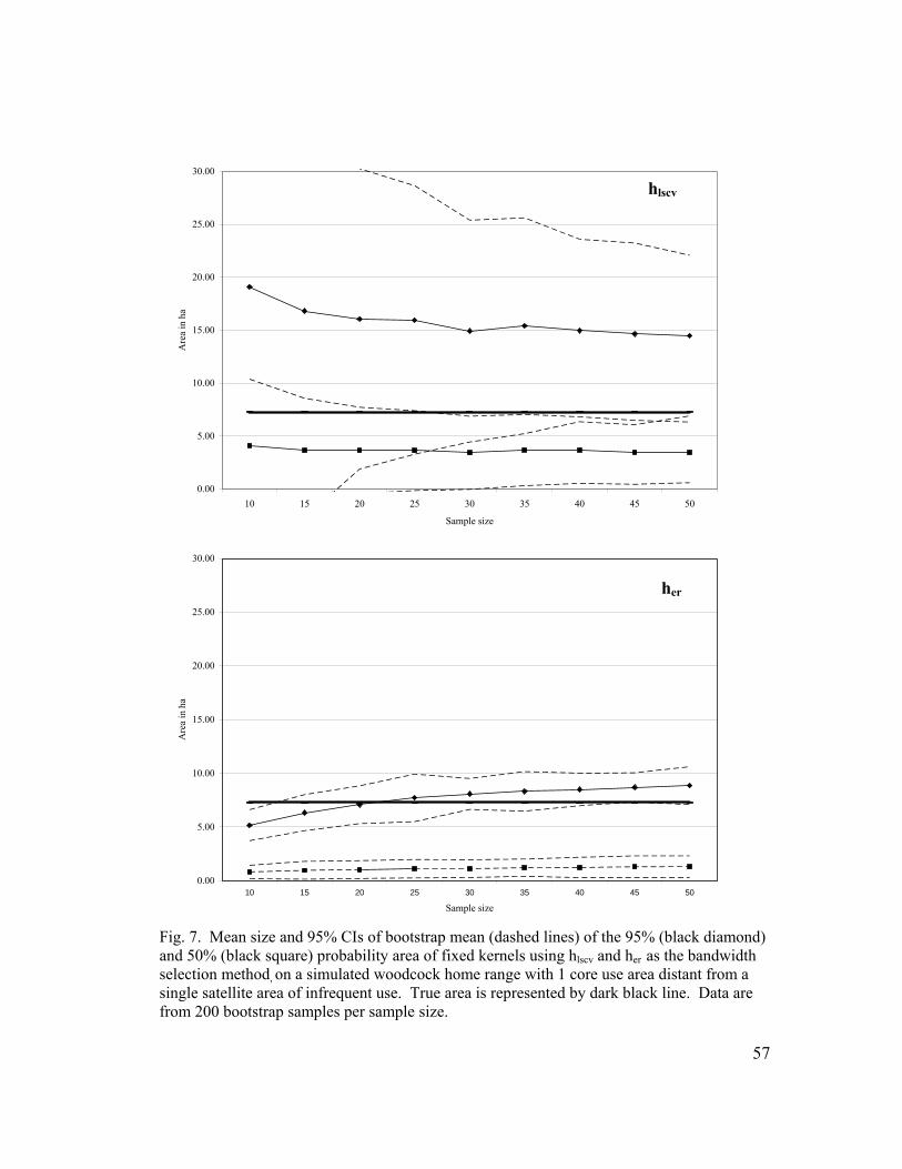
0.00
5.00
10.00
15.00
20.00
25.00
30.00
10 15 20 25 30 35 40 45
Sample size
Are
a in
ha
0.00
5.00
10.00
15.00
20.00
25.00
30.00
10 15 20 25 30 35 40 45
Sample size
Are
a in
ha
Fig. 7. Mean size and 95% CIs of bootstrap mean (dashed lines) of the 95and 50% (black square) probability area of fixed kernels using hlscv and herselection method, on a simulated woodcock home range with 1 core use arsingle satellite area of infrequent use. True area is represented by dark blafrom 200 bootstrap samples per sample size.
hlscv
50
50
her
% (black diamond) as the bandwidth ea distant from a ck line. Data are
57
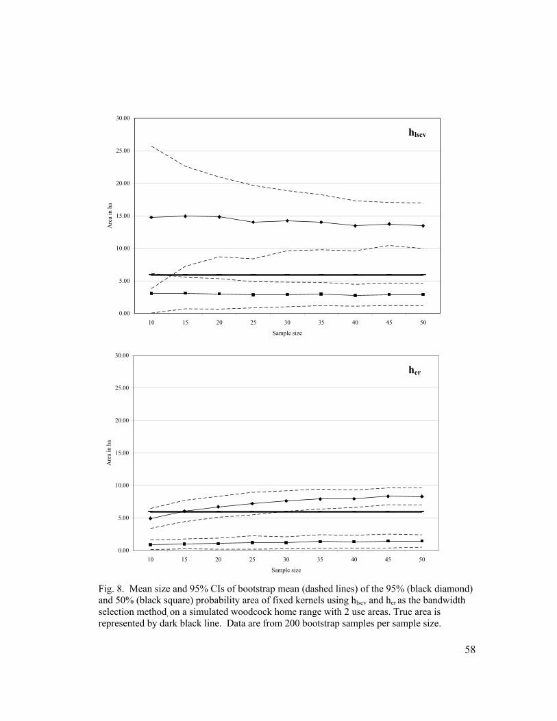
0.00
5.00
10.00
15.00
20.00
25.00
30.00
10 15 20 25 30 35 40 45
Sample size
Are
a in
ha
0.00
5.00
10.00
15.00
20.00
25.00
30.00
10 15 20 25 30 35 40 45
Sample size
Are
a in
ha
Fig. 8. Mean size and 95% CIs of bootstrap mean (dashed lines) of the 95%and 50% (black square) probability area of fixed kernels using hlscv and her asselection method, on a simulated woodcock home range with 2 use areas. Trurepresented by dark black line. Data are from 200 bootstrap samples per sam
hlscv
50
her
50
(black diamond) the bandwidth e area is ple size.
58
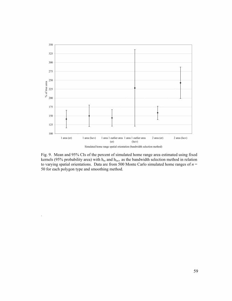
100
125
150
175
200
225
250
275
300
325
350
1 area (er) 1 area (lscv) 1 area 1 outlier area(er)
1 area 1 outlier area(lscv)
2 area (er) 2 area (lscv)
Simulated home range spatial orientation (bandwidth selection method)
% o
f tru
e ar
ea
Fig. 9. Mean and 95% CIs of the percent of simulated home range area estimated using fixed kernels (95% probability area) with her and hlscv as the bandwidth selection method in relation to varying spatial orientations. Data are from 500 Monte Carlo simulated home ranges of n = 50 for each polygon type and smoothing method. .
59