kevin constantineau jean-philippe lessard july 13, 2021
TRANSCRIPT
arX
iv:2
107.
0511
8v1
[m
ath.
DS]
11
Jul 2
021
Spatial relative equilibria and periodic solutions of the
Coulomb (n + 1)-body problem∗
Kevin Constantineau † Carlos Garcıa-Azpeitia‡ Jean-Philippe Lessard§
July 13, 2021
Abstract
We study a classical model for the atom that considers the movement of n charged particlesof charge −1 (electrons) interacting with a fixed nucleus of charge µ > 0. We show that twoglobal branches of spatial relative equilibria bifurcate from the n-polygonal relative equilibriumfor each critical values µ = sk for k ∈ [2, ..., n/2]. In these solutions, the n charges form n/h-groups of regular h-polygons in space, where h is the greatest common divisor of k and n.Furthermore, each spatial relative equilibrium has a global branch of relative periodic solutionsfor each normal frequency satisfying some nonresonant condition. We obtain computer-assistedproofs of existence of several spatial relative equilibria on global branches away from the n-polygonal relative equilibrium. Moreover, the nonresonant condition of the normal frequenciesfor some spatial relative equilibria is verified rigorously using computer-assisted proofs.
AMS Subject Classification: 70F10, 65G40, 47H11, 34C25, 37G40Keywords: Coulomb potential, N-body problem, relative equilibria, periodic solutions
1 Introduction
The Thomson problem is a classical model to study a configuration of n electrons, constrained to theunit sphere, that repel each other with a force given by Coulomb’s law. Thomson posed the problemin 1904 as an atomic model, later called the plum pudding model [13]. Without loss of generalitywe can assume that the elementary charge of an electron is e = −1, its mass is m = 1, and theCoulomb constant is 1. We wish to analyze another classical model for the atom that considers themovement of n charged particles with negative charge −1 (electrons) interacting with a fixed nucleuswith positive charge µ. Since electrons and protons have equal charges with different signs, for anon-ionized atom we consider that µ = n. By supposing that the gravitational forces are smallerthan Coulomb’s forces, the system of equations describing the movement of the charges is
qj = −µqj
‖qj‖3+
n−1∑
i=0 (i6=j)
qj − qi
‖qj − qi‖3, qj ∈ R
3, j = 0, ..., n− 1, (1)
where the first term of the force represents the interaction with the fixed nucleus.
∗Data sharing not applicable to this article as no datasets were generated or analysed during the current study†McGill University, Department of Mathematics and Statistics, 805 Sherbrooke Street West, Montreal, QC, H3A
0B9, Canada. [email protected]‡IIMAS, Universidad Nacional Autonoma de Mexico, Apdo. Postal 20-726, C.P. 01000, Mexico D.F., Mexico.
[email protected]§McGill University, Department of Mathematics and Statistics, 805 Sherbrooke Street West, Montreal, QC, H3A
0B9, Canada. [email protected]
1
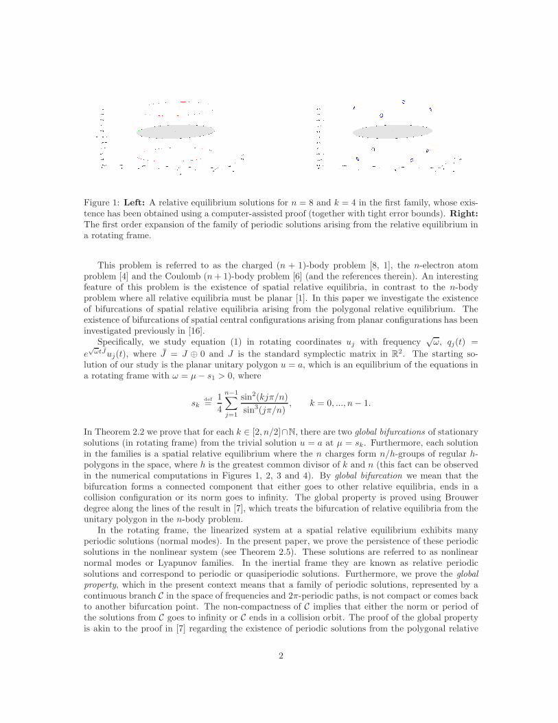
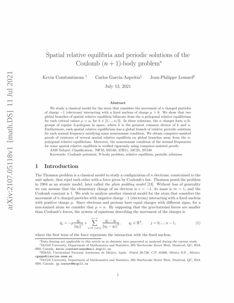
Figure 1: Left: A relative equilibrium solutions for n = 8 and k = 4 in the first family, whose exis-tence has been obtained using a computer-assisted proof (together with tight error bounds). Right:The first order expansion of the family of periodic solutions arising from the relative equilibrium ina rotating frame.
This problem is referred to as the charged (n + 1)-body problem [8, 1], the n-electron atomproblem [4] and the Coulomb (n+ 1)-body problem [6] (and the references therein). An interestingfeature of this problem is the existence of spatial relative equilibria, in contrast to the n-bodyproblem where all relative equilibria must be planar [1]. In this paper we investigate the existenceof bifurcations of spatial relative equilibria arising from the polygonal relative equilibrium. Theexistence of bifurcations of spatial central configurations arising from planar configurations has beeninvestigated previously in [16].
Specifically, we study equation (1) in rotating coordinates uj with frequency√ω, qj(t) =
e√ωtJuj(t), where J = J ⊕ 0 and J is the standard symplectic matrix in R2. The starting so-
lution of our study is the planar unitary polygon u = a, which is an equilibrium of the equations ina rotating frame with ω = µ− s1 > 0, where
skdef
=1
4
n−1∑
j=1
sin2(kjπ/n)
sin3(jπ/n), k = 0, ..., n− 1.
In Theorem 2.2 we prove that for each k ∈ [2, n/2]∩N, there are two global bifurcations of stationarysolutions (in rotating frame) from the trivial solution u = a at µ = sk. Furthermore, each solutionin the families is a spatial relative equilibrium where the n charges form n/h-groups of regular h-polygons in the space, where h is the greatest common divisor of k and n (this fact can be observedin the numerical computations in Figures 1, 2, 3 and 4). By global bifurcation we mean that thebifurcation forms a connected component that either goes to other relative equilibria, ends in acollision configuration or its norm goes to infinity. The global property is proved using Brouwerdegree along the lines of the result in [7], which treats the bifurcation of relative equilibria from theunitary polygon in the n-body problem.
In the rotating frame, the linearized system at a spatial relative equilibrium exhibits manyperiodic solutions (normal modes). In the present paper, we prove the persistence of these periodicsolutions in the nonlinear system (see Theorem 2.5). These solutions are referred to as nonlinearnormal modes or Lyapunov families. In the inertial frame they are known as relative periodicsolutions and correspond to periodic or quasiperiodic solutions. Furthermore, we prove the globalproperty, which in the present context means that a family of periodic solutions, represented by acontinuous branch C in the space of frequencies and 2π-periodic paths, is not compact or comes backto another bifurcation point. The non-compactness of C implies that either the norm or period ofthe solutions from C goes to infinity or C ends in a collision orbit. The proof of the global propertyis akin to the proof in [7] regarding the existence of periodic solutions from the polygonal relative
2
Figure 2: Left: A relative equilibrium solutions for n = 9 and k = 3 in the first family, whose exis-tence has been obtained using a computer-assisted proof (together with tight error bounds). Right:The first order expansion of the family of periodic solutions arising from the relative equilibrium ina rotating frame.
equilibrium a, and is obtained by means of the SO(2)× S1-equivariant degree developed in [10].The result of Theorem 2.5 holds when some non-resonance assumptions (Definition 2.4) on the
normal frequencies of the spatial relative equilibrium are satisfied. A main contribution of thepresent paper is the implementation of computer-assisted proofs to validate global branches of spatialrelative equilibria and also the non-resonance assumption, which is required to obtain the existenceof families of periodic solutions arising from them. In Section 3, we present the general approach(a Newton-Kantorovich type theorem, see Theorem 3.1) used to obtain the different computer-assisted proofs. This theorem is used to validate the spatial relative equilibria (in Section 3.1)and its normal frequencies (in Section 3.2) to verify the conditions of Theorem 2.5. Figures 1 and 2contain an example of spatial relative equilibria whose existence has been obtained using a computer-assisted proof (together with tight error bounds) and for which the non-resonance condition has beenrigorously verified. Similar computer-assisted proofs were carried on for each (non black) point inFigures 3 and 4.
2 Existence of periodic solutions arising from spatial relative
equilibria
We assume that: the gravitational forces are much smaller than Coulomb’s forces, the charge in thecenter is µ > 0, the n charges have charge −1, the mass of the charges is m = 1 and the Coulombconstant is κ = 1. We also assume that the position of the central charge is fixed at the centerand the positions of the n charges are determined by q(t) = (q0(t), ..., qn−1(t)) with qj(t) ∈ R3 forj = 0, ..., n− 1. Under these assumptions, the system satisfies the Newtonian equation
u(t) = ∇U(q(t)), (2)
where U(q) is the potential energy given by
U(q)def
=n−1∑
j=0
µ
‖qj‖−∑
i<j
1
‖qj − qi‖,
where the first term represents the interaction with the fixed center.Let J = J ⊕ 0, where J is the standard symplectic matrix in R2. In rotating coordinates,
qj(t) = e√ωtJuj(t), the system of equations becomes uj + 2
√ωJuj = ∇uj
V (u), where V is the
3
augmented potential
V (u) =ω
2
n−1∑
j=0
∥
∥Iuj
∥
∥
2+
n−1∑
j=0
µ
‖uj‖−
∑
i<j
1
‖uj − ui‖,
where I = −J2 = 1⊕ 1⊕ 0. Let u = (u0, ..., un−1) and J = J ⊕ ...⊕ J , the system of equation reads
u+ 2√ωJ u = ∇V (u). (3)
Let Sn be the group of permutations of {0, 1, ..., n− 1} and Dn be the subgroup generated bythe permutations ζ(j) = j + 1 and κ(j) = n− j mod n. We define the action of γ ∈ Sn in R3n as
ρ(γ)(u0, u1, ..., un−1) = (uγ(0), uγ(1), ..., uγ(n−1)). (4)
Notice that this is a left action only if the product on Sn is defined according to the oppositeconvention that σ1σ2
def
= σ2 ◦ σ1. Clearly the potential V is Sn-invariant. On the other hand, whilethe potential U(u) is O(3)-invariant, the potential V (u) is only invariant under the action of thenormalizer O(2)× Z2 of SO(2) ⊂ O(3).
We conclude that V (u) is G-invariant with
Gdef
= Sn ×O(2)× Z2.
The explicit action of the elements θ, κy ∈ O(2) and κz ∈ Z2 in the components of u is given by
θuj = e−J θuj , κyuj = Ryuj, κzuj = Rzuj,
whereRy = 1⊕−1⊕ 1, Rz = 1⊕ 1⊕−1.
2.1 The polygonal relative equilibrium
The polygon a = (a0, ..., an−1), where
aj =(
eijζ , 0)
∈ C× R, ζdef
= 2π/n,
is a critical point of V (u;ω) for ω = µ− s1 > 0. This follows from the identity
∇ujV (a) = ωaj − µaj +
n−1∑
i=0 (i6=j)
aj − ai
‖aj − ai‖3= aj (ω − µ+ s1) ,
where we have used that
n−1∑
i=0 (i6=j)
aj − ai
‖aj − ai‖3= aj
n−1∑
i=0 (i6=j)
1− eijζ
‖1− eijζ‖3= aj
1
4
n−1∑
j=1
1
sin(jπ/n)= ajs1.
2.2 Bifurcation of spatial relative equilibria
Hereafter we assume that ω = µ − s1 and we denote the dependence of the potential V in theparameter µ as V (u;µ). Thus the polygon u = a is a trivial solution of ∇V (u;µ) = 0 with isotropygroup Ga generated by
ζ = (ζ, ζ, e) , κy = (κ, κy, e) , κz = (e, e, κz) ∈ Sn ×O(2)× Z2,
4
where e represents the identity element. As a consequence of the continuous action of SO(2), theorbit of the polygonal equilibrium a is one dimensional. Thus the generator of the SO(2)-orbit of ais −J a, which belongs to the kernel of D2V (u).
Given that Ga fixes a, then D2V (a) is Ga-equivariant and, by Schur’s lemma, it has the sameeigenvalue in each irreducible representations under the action of Ga. The spatial irreducible repre-sentations of Ga are obtained in section “8.4. The problem of n-charges” in the paper [8]. DefineVk as the subspace generated by
vk =(
v0k, , ..., vn−1k
)
∈ R3n,
where vjk = (0, 0, cos jkζ) for k ∈ [0, n/2] ∩ N and vjk = (0, 0, sin jkζ) for k ∈ (n/2, n− 1] ∩ N, thenthe irreducible Ga-representations are given by Vk for k = 0, n/2 and Vk ⊕Vn−k for k ∈ [1, n/2)∩N.
Specifically, using the isomorphism
avk + bvn−k ∈ Vk ⊕ Vn−k → a+ ib ∈ C,
the action of ζ, κy, κz ∈ Ga in z = a+ ib ∈ C is given by
ζz = eikζz, κyz = z, κzz = −z. (5)
For k = 0, n/2 the action in Vk ≃ R is the same as before but with z ∈ R. For instance, fork ∈ (0, n/2) ∩ N we have that
ζ (avk + bvn−k) = e−J ζζ · (avk + bvn−k)
= {(0, 0, a cos(jk + k)ζ − b sin(jk + k)ζ)}nj=1
= (a cos kζ − b sinkζ) vk + (b cos kζ + a sin kζ) vn−k.
Hence, we obtain that
ζz = (a cos kζ − b sinkζ) + i (b coskζ + a sin kζ) = eikζz.
In section “8.4. The problem of n-charges” in the paper [8] is proven that the eigenvalue ofHessian D2V (a) in each irreducible representation Vk for k = 0, n/2 and Vk ⊕ Vn−k is −µ + sk.For sake of completeness we present a short proof of this fact. For k ∈ {0, ..., n − 1}, we defineTk : R → Wk as
Tk(w) = (0, 0, n−1/2eikζw, ..., 0, 0, n−1/2enikζw) with
Wk = {(0, 0, eikζw, ..., 0, 0, enikζw) ∈ C3n : w ∈ R}.
Since Wk = Vk ⊕ iVn−k, the result follows from the invariance of the subspaces Wk of D2V (a) withthe following computation.
Proposition 2.1. For k ∈ {0, ..., n− 1}, we have
D2V (a)Tk(w) = Tk((−µ+ sk)w).
Proof. Let Aij be the 3 × 3 minor blocks of the Hessian D2V (a) = (Aij)nij=1. The fact that a is a
planar configuration implies that the matrices Aij are block diagonal
Aij = diag(Aij , aij),
5
where Aij is a 2 × 2 matrix. For our purpose we only need to compute the numbers aij . Letdij = |ui − uj | be the distance between ui = (xi, yi, zi) and uj = (xj , yj , zj). For i 6= j we have that∂zi(d
−1ij ) = −∂zj (d
−1ij ) and
aij = −∂zj∂zid−1ij |u=a = ∂2
zid−1ij |u=a = −d−3
ij |u=a = − (2 sin((i − j)ζ/2))−3
. (6)
For i = j the number aii satisfies
aii = ∂2zi
(
µ
‖uj‖
)
uj=aj
−n−1∑
j=0 (j 6=i)
(
∂2zid
−1ij
)
uj=aj
= −µ−n−1∑
j=0 (j 6=i)
aij .
Now we need to denote to the component wi ∈ C3 of the vector w = (w0, ..., wn−1) ∈ C3n as[w]i = wi. From the definitions we have that
[D2V (a)Tk(w)]l =
0, 0, n−1/2n−1∑
j=0
aljeijkζw
.
Since alj = a0(j−l) with (j−l) ∈ {0, ..., n−1}modulus n. From the equality aljeijkζ = eilkζ
(
a0(j−l)ei(j−l)kζ
)
we have that[D2V (a)Tk(w)]l =
(
0, 0, n−1/2eilkζbkw)
= [Tk(bkw)]l ,
where
bk =
n−1∑
j=0
a0jeijkζ = −µ+
n−1∑
j=1
(
eijkζ − 1)
a0j ,
because a00 = −µ−∑n−1j=0 a0j . Finally, using (6), we obtain that
n−1∑
j=1
(
eijkζ − 1)
a0j =n−1∑
j=1
2 sin2(kjζ/2)
23 sin3(jζ/2)= sk.
According to [8], for k ∈ [2, n/2), the Hessian D2V (u; sk) has no additional zero-eigenvalues tothe double zero-eigenvalue corresponding to the subspace Vk ⊕ Vn−k and the simple zero-eigenvaluecorresponding to the generator of the xy-rotations −J a. That is,
kerD2V (a; sk) = Vk ⊕ Vn−k ⊕ J a.
In order to prove the existence of solutions ∇V (u;µ) = 0 bifurcating from the trivial solution u = awhen the parameter µ crosses sk, we consider the fixed point spaces of two subgroups
H1 = Z2 (κy) , H2 = Z2 (κyκz) .
That is, let ∇V Hj : Fix(Hj) → Fix(Hj) be the restriction of ∇V to the fixed point space of Hj
for j = 1, 2, we will show that the restricted maps ∇V Hj for j = 1, 2 have the advantage that thezero-eigenvalue −J a is not present in D2V Hj and that the double zero-eigenvalue −µ+ sk becomessimple.
The fixed point space of R3n under the action of H1 satisfies the symmetries
u0 = Ryu0, un/2 = Ryun/2, uj = Ryun−j , (7)
and of H2
u0 = RzRyu0, un/2 = RzRyun/2, uj = RzRyun−j . (8)
6
Theorem 2.2. For each k ∈ [2, n/2]∩N, there are two global bifurcations of solutions of ∇V (u;µ) =0 from the trivial solution u = a at µ = sk, one denoted by Fk
1 with symmetries (7) and anotherdenoted by Fk
2 with symmetries (8). Furthermore, the relative equilibria in both families are formedby n/h-groups of regular h-polygons, where h is the greatest common divisor of k and n.
Proof. We look for bifurcation of solutions of ∇V H1(u;µ) = 0 from the trivial solution u = a atµ = sk. Using that kerD2V (a; sk) = Vk ⊕Vn−k ⊕ J a, it is easy to see that vn−k ∈ Vn−k and J a donot satisfy the symmetry (7), which implies that they do not belong to Fix(H1). Thus the kernel ofD2V H1(a; sk) is one dimensional and generated by vk ∈ Vk. The eigenvalue −µ+ sk correspondingto the eigenvector vk ∈ Vk crosses zero at µ = sk. Using Brouwer degree as in section “3. Bifurcationtheorem” in [7], we can prove the existence of a global bifurcation of solutions of ∇V H1(u;µ) = 0from the trivial solution u = a at µ = sk. Furthermore, since ζn/h leaves the subspace Vk fixed,
because ζn/hz =(
eik2π/n)n/h
z = z according to (5), then the family of solutions Fk1 arising from
µ = sk is fixed by the group Zh generated by ζn/h. This implies that the solution is formed byn/h-polygons (see [7] for details). The proof in the case k = n/2 and H2 is analogous, the only keydifference is that
kerD2V H2(a; sk) = kerD2V (a; sk) ∩ Fix(H2) = Vn−k,
because vk ∈ Vk and J a do not satisfy the symmetry (8), and they do not belong to Fix(H2).
The polygon a is a relative equilibrium only when ω = µ − s1 > 0, which requires that µ > s1.In a slightly different context it was noticed by R. Moeckel [15] that the condition µ = n > s1holds only for n < 473. An interesting consequence of this fact is that for a non-ionized atom then-polygon is a relative equilibrium only for an atomic number less than 473. We obtain numericallythe additional inequalities s1 < n < s2 for n = 3 and n ≥ 12, s2 < n < s3 for n = 4, 5, 8, 9, 10, 11and s3 < n < s4 for n = 6, 7. Since the bifurcations of relative equilibria arising from the polygonsat µ = sk are subcritical, for instance, one can deduce from these inequalities that it is unlikely tofind a relative equilibrium with µ = n in the bifurcation from s1 for the cases n = 4, ..., 11.
2.3 Periodic solutions arising from spatial relative equilibria
Now we turn the attention to the analysis of non-trivial 2π/ν-periodic solutions of (3) arising froma spatial relative equilibrium (u0;µ0), which for the present paper belongs to the families Fk
1 orFk2 . For the validation of the hypotheses necessary to obtain the periodic solutions we will use
the computer-assisted proof technique of Section 3. These hypotheses are easier to verify in theequivalent system
(
uv
)
=
(
v−2
√µ− s1J v +∇V (u;µ)
)
. (9)
The linearization of equation (9) at a spatial relative equilibrium (u0;µ0) is
(
u
v
)
= L(u0;µ0)
(
u
v
)
, L(u0;µ0)def
=
(
0 ID2V (u0;µ) −2
√µ0 − s1J
)
.
Notice that λ is an eigenvalue of L(u0;µ0) with eigenvector (u, v) if and only if v = λu and
−2√µ0 − s1J v +D2V (u0;µ0)u = λv.
This condition is equivalent to u ∈ ker M(λ), where
M(λ) = −λ2I − 2√µ0 − s1λJ +D2V (u0;µ0).
7
Remark 2.3. Since M(λ) = M(−λ)T , then det M(λ) = det M(−λ) is an even real polynomial inλ. Thus λ,−λ,−λ are eigenvalues of L(u0;µ0) if λ ∈ C is an eigenvalue of L(u0;µ0). Actually, thisis an immediate consequence of the fact that the matrix L(u0;µ0) is a reformulation, as first ordersystem for positions and velocities, of a Hamiltonian matrix [14].
The purely imaginary eigenvalues λ = iν0 of L(u0;µ0) give the (normal) frequencies of theperiodic solutions of the linearized system. The periodic solutions of the linearized system persistin the nonlinear system (non-linear normal modes) under the assumptions of the Lyapunov centertheorem [14]. The main assumption is that iν0 is non-resonant, which means that the eigenvalue iν0is a simple eigenvalue of L(u0;µ0) and ilν0 is not an eigenvalue of L(u0;µ0) for any integer l 6= 1.
The classical Lyapunov center theorem cannot be applied directly because the equilibrium a isnot isolated and zero is always an eigenvalue of L(u0;µ0) due to the SO(2)-action. Other equivariantversions of the Lyapunov theorem consider these circumstances such as [10] and [19]. In order touse a simple version of those results, we make the following definition.
Definition 2.4. We say that iν0 is a SO(2)-nonresonant eigenvalue of L(u0;µ0) if iν0 is a simpleeigenvalue of L(u0;µ0), 0 is a double eigenvalue of L(u0;µ0) due to the action of the group SO(2),and ilν0 is not an eigenvalue of L(u0;µ0) for integers l ≥ 2.
In the case that iν0 is a SO(2)-nonresonant eigenvalue of L(u0;µ0) with eigenvector (u, v), thefirst order asymptotic expansion of the family of periodic solutions is given by
u(t) = u0 + εRe(eiν0tu) +O(ε2).
We use this fact to produce the illustrations of the periodic solutions in Figures 1 and 2.
Theorem 2.5. A relative equilibrium (u0;µ0) has a global family of 2π/ν-periodic solutions arisingfrom u0 with initial frequency ν = ν0 when L(u0;µ0) has a SO(2)-nonresonant eigenvalue iν0.
Proof. Looking for 2π/ν-periodic solutions of the equation u+2√µ− s1J u = ∇V (u;µ) is equivalent
to look for zeros x(t) = u(tν) of the map
F(x;µ, ν) = −ν2x− 2√µ− s1J νx+∇V (u;µ) : H2
2π × R2 → L2
2π.
We consider that µ = µ0 is fixed, then u0 satisfies F(u0;µ0, ν) = ∇V (u0;µ0) = 0. The linearizationDF(u0;µ0, ν) in Fourier components x =
∑
xleilt is DF(u0;µ0, ν) =
∑
l∈ZM(lν)xle
ilt, where
M(ν) = M(iν) = ν2I − 2√µ0 − s1iνJ +D2V (u0;µ0)
is a self-adjoint matrix. Thus, the assumption that iν0 is SO(2)-nonresonant implies that kerM(0)is generated by J a, ν0 is a simple zero of detM(ν0) and M(lν0) is invertible for integers l ≥ 2.
Therefore, the kernel of the linearized operator DF(u0;µ0, ν0) consists exactly of J a and thereal and imaginary parts of eitw with w ∈ kerM(ν0). These are the necessary hypotheses in orderto prove the bifurcation theorem in Section 6 in [8]. We proceed analogously: Let σ be the sign ofthe determinant of D2V (u0;µ0) in the orthogonal complement to J a (the generator of the SO(2)-orbit). Under the non-resonance assumption, we have that σ 6= 0. Let n(ν) be the Morse index ofthe self-adjoint matrix M(ν). Since M(lν0) is invertible for integers l ≥ 2, according to Section 6 in[8], we have that the SO(2)× S1-equivariant index of F(x;µ0, ν) at the orbit of u0 is σn(ν)(Z1). In[10] is proven that a global bifurcation of periodic solutions exists if this index changes. The resultfollows from the fact that ν0 is a simple root of the polynomial detM(ν) = 0, i.e. the Morse indexn(ν) necessarily changes at ν0.
Remark 2.6. The local existence of the family of periodic solutions can be proven using Poincaresections as in [19]. It is also possible to use equivariant degree theory to prove the existence of thefamily of periodic solutions even for SO(2)-resonant eigenvalues, but for validating the hypotheseswith computer-assisted proofs it is simple to consider the case of SO(2)-nonresonant eigenvalues.
8
3 Computer-assisted proofs of relative equilibria
In this section, we use a pseudo-arclength continuation method (e.g. see [11]) to numerically computebranches of steady states in the families Fk
1 and Fk2 . Along with the numerical continuation, we obtain
computer-assisted proofs of the equilibria and we verify the hypotheses of Theorem 2.5 to concludethe existence of families of periodic orbits. This is done using a Newton-Kantorovich type theorem,which is similar to the Krawczyk operator’s approach [17, 12] and the interval Newton method [18].The presented formulation is inspired by the so-called radii polynomial approach (e.g. see [5, 9, 2]),which is also a variant of the Newton-Kantorovich Theorem.
Consider a finite dimensional Banach space X (in our context X = RN or X = CN , for someN ∈ N). Choose a norm ‖ · ‖X on X . Given a point y ∈ X and a radius r > 0, denote byBr(y) = {x ∈ X : ‖y − x‖ < r} the open ball of radius r centered at y. Similarly, denote by Br(y)the closed ball.
Theorem 3.1. Let U ⊂ X be an open set. Consider a Frechet differentiable mapping F : U → Xand fix a point u ∈ U (an approximate zero of F ). Let A be an approximate inverse of the Jacobianmatrix DF (u) (that is ‖I − ADF (u)‖B(X) ≪ 1), where I is the identity on X and where ‖ · ‖B(X)
denotes the operator/matrix norm induced by the norm ‖ · ‖X on X. Fix r∗ > 0. Suppose that thebounds Y, Z = Z(r∗) > 0 satisfy
‖AF (u)‖X ≤ Y and supz∈Br∗ (u)
‖I −ADF (z)‖B(X) ≤ Z.
Definep(r) = (Z − 1)r + Y. (10)
If there exists r0 ∈ (0, r∗] such that p(r0) < 0, then there is a unique u ∈ Br0(u) such that F (u) = 0.
Proof. Define the Newton-like operator T : U → X by
T (u) = u−AF (u),
and note that DT (u) = I − ADF (u). The idea of the proof is to show that T : Br0(u) → Br0(u) isa contraction. Consider r0 ∈ (0, r∗] such that p(r0) < 0. Then Zr0 + Y < r0, and since r0 is notzero, we have that Z ≤ Z + Y
r0< 1. For x, y ∈ Br0(u) we use the Mean Value Inequality to get that
‖T (u)− T (v)‖X ≤ supz∈Br0
(x)
‖DT (z)‖B(X)‖u− v‖X
= supz∈Br0
(u)
‖I −ADF (z)‖B(X)‖u− v‖X
≤ supz∈Br∗(u)
‖I −ADF (z)‖B(X)‖u− v‖X
≤ Z‖u− v‖X .
Since Z < 1, T is a contraction on Br0(u). To see that T maps the closed ball into itself (in fact inthe open ball) choose u ∈ Br0(u), and observe that
‖T (u)− u‖X ≤ ‖T (u)− T (u)‖X + ‖T (u)− u‖X≤ Z‖u− u‖X + ‖AF (u)‖X≤ Zr0 + Y = p(r0) + r0 < r0,
9
which shows that T (u) ∈ Br0(u) for all u ∈ Br0(u). It follows from the contraction mapping theoremthat there exists a unique u ∈ Br0(u) such that T (u) = u ∈ Br0(u). Since Z < 1, we get
‖I −ADF (u)‖B(X) ≤ supz∈Br∗(u)
‖I −ADF (z)‖B(X) ≤ Z < 1,
and hence ADF (u) is invertible. From this we get that A is invertible. By invertibility of A and bydefinition of T , the fixed points of T are in one-to-one correspondence with the the zeros of F . Weconclude that there is a unique u ∈ Br0(u) such that F (u) = 0.
In practice, we perform the rigorous computation of the bounds Y and Z with interval arithmetic[18] in MATLAB using the library INTLAB [20].
3.1 The first family of spatial relative equilibria
To proceed with the computer-assisted proof of the relative equilibria we need to find an explicitrepresentation for ∇V H1 : Fix(H1) → Fix(H1). For this purpose, we define the subspace
X1 ={
u = (u0, u1, ...., u[n/2]) ∈ R3 × ...× R
3 : uj = (xj , 0, zj) ∈ R3, j = 0, n/2
}
and the isomorphismι1 : X1 → Fix(H1), ι1(u) = (u0, u1, ...., un) ,
given by uj = uj for j ∈ [0, n/2]∩N and uj = Ryun−j for j ∈ (n/2, n− 1]∩N. Therefore, the zerosof ∇V H1 : Fix(H1) → Fix(H1) correspond to the zeros of
F1def
= ι−11 ◦ ∇V H1 ◦ ι1 : X1 → X1.
More explicitly, we have that
F1 = (f0, f1, ...., f[n/2]) : X1 → X1, (11)
where
fj(u;µ) = (µ− s1) Iuj − µuj
‖uj‖3+
∑
0≤i≤n/2(i6=j)
uj − ui
‖uj − ui‖3+
∑
0<i<n/2
uj −Ryui
‖uj −Ryui‖3.
This fact can be verified directly. We conclude that the families of solutions of F1(u;µ) = 0 are thecritical solutions of V (u;µ) with u = ι1 (u) ∈ Fix(H1).
To compute numerically the family Fk1 (that is solutions of F1(u;µ) = 0), we apply the pseudo-
arclength continuation method [11], which we now briefly review. Denote Ndef
= 3([n/2] + 1) − 2,so that X1
∼= RN . Using that notation, F1 : R
N+1 → RN . The idea of the pseudo-arclength
continuation is to treat the parameter µ as a variable, to set Udef
= (u;µ) ∈ RN+1 and perform acontinuation with respect to the pseudo-arclength parameter. The process begins with a solution U0
(exact or numerical given within a prescribed tolerance). To produce a predictor, which will serveas an initial condition to Newton’s method, we compute a tangent vector U0 (of unit length) to thecurve at U0. It can be computed using the formula
DUF1(U0)U0 =
[
DuF1(U0)∂F1
∂µ(U0)
]
U0 = 0 ∈ RN .
Denoting the pseudo-arclength parameter by ∆s > 0, set the predictor to be
U1def
= U0 +∆sU0 ∈ RN+1.
10
The corrector step then consists of converging back to the solution curve on the hyperplane perpen-dicular to the tangent vector U0 which contains the predictor U1. The equation of this plan is givenby E(U)
def
= (U − U1) · U0 = 0. Then, we apply Newton’s method to the new function
U 7→(
E(U)F1(U)
)
(12)
with the initial condition U1 in order to obtain a new solution U1 given again within a prescribedtolerance. We reset U1 7→ U0 and start over. At each step of the algorithm, the function defined in(12) changes since the plane E(U) = 0 changes. With this method, it is possible to continue pastfolds. Repeating this procedure iteratively produces a branch of solutions.
We initiate the numerical continuation from the trivial solutions u = ι−11 (a) at µ = sk. More
explicitly, at the beginning, we set U0 = (ι−11 (a), sk) ∈ RN+1. Then, along the continuation, we use
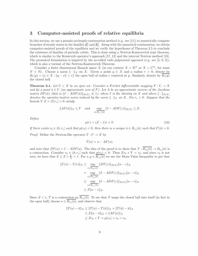
Theorem 3.1 to verify the existence (with tight rigorous error bounds) of several solutions of F1 = 0(with F1 defined in (11)), hence yielding spatial relative equilibria in the family Fk
1 . See Figure 3 forplots of several continuations.
A similar analysis and numerical implementation have been implemented for the family of solu-tions Fk
2 satisfying the symmetry (8), by using instead the map
F2(u;µ) = (f0, f1, ...., f[n/2]) : X2 → X2,
X2 ={
u = (u0, u1, ...., u[n/2]) : uj = (xj , 0, 0) ∈ R3, j = 0, n/2
}
,
where
fj(u;µ) = (µ− s1) Iuj − µuj
‖uj‖3+
∑
0≤i≤n/2(i6=j)
uj − ui
‖uj − ui‖3+
∑
0<i<n/2
uj −RzRyui
‖uj −RzRyui‖3.
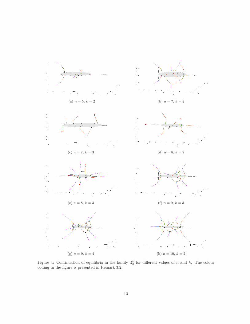
See Figure 4 for plots of several continuations in the family Fk2 .
Remark 3.2 (Colour coding for Figures 3 and 4). The colour coding for the presentation of therelative equilibrium solutions in Figures 3 and 4 is as follows. Each branch going from green to redrepresents the main branch, while each cyan to purple branch portrays a branch born from a secondarybifurcation from the main branch. The points in the following colours were not successfully validatedwith computer-assisted proofs for three reasons: (Blue) unable to verify the relative equilibria, (Black)unable to verify the eigenvalues and (Orange) unable to verify the nonresonance of the eigenvalues.
Remark 3.3. All the spatial relative equilibria are unstable near the polygon because the polygonis unstable according to the computations obtained in [8]. Unfortunately, we were not able to findlinearly stable solutions from the numerical exploration carried on for the branches, so all the relativeequilibria that we computed are unstable.
3.2 A computer-assisted validation of the spectra
The existence of non-trivial 2π/ν-periodic solutions of (3) arising from a spatial relative equilibrium(u0;µ0) relies on the validation of the hypotheses of Theorem 2.5; namely, to verify the existence of aSO(2)-nonresonant eigenvalue of L(u0;µ0) (see Definition 2.4). Now we turn our attention to provethis hypothesis by means of Theorem 3.1. Recall from Remark 2.3 that λ,−λ,−λ are eigenvaluesof L(u0;µ0) if λ ∈ C is an eigenvalue of L(u0;µ0). Thus, if we prove the existence of a uniqueeigenvalue λ0 in a neighbourhood Bε(iν) ⊂ C, then λ0 = iν0 for some ν0 ∈ R (i.e. λ0 must be purelyimaginary).
11
(a) n = 5, k = 2 (b) n = 7, k = 2
(c) n = 7, k = 3 (d) n = 8, k = 3
(e) n = 8, k = 4 (f) n = 9, k = 3
(g) n = 9, k = 4 (h) n = 10, k = 2
Figure 3: Continuation of equilibria in the family Fk1 for different values of n and k. The colour
coding in the figure is presented in Remark 3.2
12
(a) n = 5, k = 2 (b) n = 7, k = 2
(c) n = 7, k = 3 (d) n = 8, k = 2
(e) n = 8, k = 3 (f) n = 9, k = 3
(g) n = 9, k = 4 (h) n = 10, k = 2
Figure 4: Continuation of equilibria in the family Fk2 for different values of n and k. The colour
coding in the figure is presented in Remark 3.2.
13
Recall that the existence of the relative equilibria u0 ∈ Br0(u0) is known via a successful ap-plication of Theorem 3.1, where u0 is a numerical solution and r0 > 0 is the rigorous error bound.The validation of the eigenvalues of L(u0;µ0), which follows the approach [3], begins by finding nu-merically the eigenvalues of L(u0;µ0). Denote by λ1, . . . , λ6n the numerical eigenvalues of L(u0;µ0)(computed using the function eig.m in MATLAB, which returned the eigenvalues and their corre-sponding eigenvectors v1, . . . , v6n). Fix j ∈ {1, . . . , 6n}. Then, in order to obtain local isolation ofthe eigenpairs (λj , vj) ∈ C× C6n, we rescale the eigenvector vj as follows. Denote by k = k(j) thecomponent of vj with the largest magnitude, that is
|(vj)k| = maxℓ=1,...,6n
{|(vj)ℓ|} .
Note that k may not be unique. Then, the phase condition imposed to isolate the eigenpair (λj , vj) is(vj)k = (vj)k, where recall that vj ∈ C6n is the numerical approximation for vj . The correspondingzero finding problem is setup in the following way
Feig(v, λ)def
=
(
L(u0;µ0)v − λvv · ek − (vj)k
)
= 0, (13)
where λ and v are the eigenvalue and eigenvector, respectively, and ek is the kth vector of thecanonical basis of R6n. Without loss of generality, denote by λ1 = λ2 = 0 the two zero eigenvalues ofL(u0;µ0) due to the action of the group SO(2). For each j ∈ {3, . . . , 6n}, the rigorous enclosure ofthe eigenpair (λj , vj) is obtained by validated the existence of a solution of Feig = 0 (where the mapis defined in (13)) using Theorem 3.1. Denote by rj > 0 the radius of the ball Brj (λj , vj) ⊂ C×C6n
which contains the unique eigenpair with v · ek = (vj)k, which we denote simply by (λj , vj).For j = 3, . . . , 6n, denote by
Djdef
={
z ∈ C : |zj − λj | ≤ rj}
⊂ C
the disk which contains the true eigenvalue λj . Assume that numerically, two eigenvalues are givenby ±iν0, for some ν0 > 0. Without loss of generality, denote by λ3 and λ4 the true eigenvalues suchthat
|λ3 − iν0| ≤ r3 and |λ4 + iν0| ≤ r4.
By unicity, the true eigenvalues satisfy λ3 = iν0 and λ4 = −iν0, for some ν0 > 0 since otherwise thedisk D3 and D4 would contain more eigenpairs by the comment above (see also Remark 2.3). Henceλ3 = iν0 ∈ D3 and λ4 = iν0 ∈ D4. Denote
D def
=
6n⋃
j=5
Dj
which contains rigorously λ5, . . . , λ6n. The other four eigenvalues are given by 0, 0,±iν0. For eachspatial relative equilibria rigorously proven in Section 3.1, we verified rigorously that D ∩ iν0N = ∅(where N
def
= {ℓ ∈ Z : ℓ ≥ 2}), hence showing rigorously that the eigenvalue iν0 is a SO(2)-nonresonant eigenvalue. All of the computations were carried out in MATLAB using the libraryINTLAB [20].
Acknowledgements. JP.L. was partially supported by NSERC Discovery Grant. K.C. waspartially supported by an ISM-CRM Undergraduate Summer Scholarship. C.G.A was partiallysupported by UNAM-PAPIIT project IA100121.
14
References
[1] Felipe Alfaro Aguilar and Ernesto Perez-Chavela. Relative equilibria in the charged n-bodyproblem. The Canadian Applied Mathematics Quarterly, 10, 01 2002.
[2] Istvan Balazs, Jan Bouwe van den Berg, Julien Courtois, Janos Dudas, Jean-Philippe Lessard,Anett Voros-Kiss, J. F. Williams, and Xi Yuan Yin. Computer-assisted proofs for radiallysymmetric solutions of PDEs. J. Comput. Dyn., 5(1-2):61–80, 2018.
[3] Roberto Castelli and Jean-Philippe Lessard. A method to rigorously enclose eigenpairs ofcomplex interval matrices. In Applications of mathematics 2013, pages 21–31. Acad. Sci. CzechRepub. Inst. Math., Prague, 2013.
[4] Ian Davies, Aubrey Truman, and David Williams. Classical periodic solution of the equal-mass2n-body problem, 2n-ion problem and the n-electron atom problem. Phys. Lett. A, 99(1):15–18,1983.
[5] Sarah Day, Jean-Philippe Lessard, and Konstantin Mischaikow. Validated continuation forequilibria of PDEs. SIAM J. Numer. Anal., 45(4):1398–1424 (electronic), 2007.
[6] Marco Fenucci and Angel Jorba. Braids with the symmetries of Platonic polyhedra in theCoulomb (N +1)-body problem. Commun. Nonlinear Sci. Numer. Simul., 83:105105, 12, 2020.
[7] C. Garcıa-Azpeitia and J. Ize. Global bifurcation of polygonal relative equilibria for masses,vortices and dNLS oscillators. J. Differential Equations, 251(11):3202–3227, 2011.
[8] C. Garcıa-Azpeitia and J. Ize. Global bifurcation of planar and spatial periodic solutions fromthe polygonal relative equilibria for the n-body problem. J. Differential Equations, 254(5):2033–2075, 2013.
[9] Allan Hungria, Jean-Philippe Lessard, and J. D. Mireles James. Rigorous numerics for analyticsolutions of differential equations: the radii polynomial approach. Math. Comp., 85(299):1427–1459, 2016.
[10] Jorge Ize and Alfonso Vignoli. Equivariant degree theory, volume 8 of De Gruyter Series inNonlinear Analysis and Applications. Walter de Gruyter & Co., Berlin, 2003.
[11] H. B. Keller. Lectures on numerical methods in bifurcation problems, volume 79 of Tata Instituteof Fundamental Research Lectures on Mathematics and Physics. Published for the Tata Instituteof Fundamental Research, Bombay, 1987. With notes by A. K. Nandakumaran and MythilyRamaswamy.
[12] R. Krawczyk. Newton-Algorithmen zur Bestimmung von Nullstellen mit Fehlerschranken. Com-puting (Arch. Elektron. Rechnen), 4:187–201, 1969.
[13] Tim LaFave. Correspondences between the classical electrostatic thomson problem and atomicelectronic structure. Journal of Electrostatics, 71(6):1029 – 1035, 2013.
[14] Kenneth R. Meyer and Glen R. Hall. Introduction to Hamiltonian dynamical systems and theN -body problem, volume 90 of Applied Mathematical Sciences. Springer-Verlag, New York, 1992.
[15] Richard Moeckel. On central configurations. Mathematische Zeitschrift, 205(1):499–517, sep1990.
15
[16] Richard Moeckel and Carles Simo. Bifurcation of spatial central configurations from planarones. SIAM Journal on Mathematical Analysis, 26(4):978–998, jul 1995.
[17] R. E. Moore. A test for existence of solutions to nonlinear systems. SIAM J. Numer. Anal.,14(4):611–615, 1977.
[18] Ramon E. Moore. Interval analysis. Prentice-Hall Inc., Englewood Cliffs, N.J., 1966.
[19] F. J. Munoz Almaraz, E. Freire, J. Galan, E. Doedel, and A. Vanderbauwhede. Continuationof periodic orbits in conservative and Hamiltonian systems. Phys. D, 181(1-2):1–38, 2003.
[20] S.M. Rump. INTLAB - INTerval LABoratory. In Tibor Csendes, editor, Develop-ments in Reliable Computing, pages 77–104. Kluwer Academic Publishers, Dordrecht, 1999.http://www.ti3.tu-harburg.de/rump/.
16