kernsmoothirt: an r package for kernel smoothing in item ... · 2 kernsmoothirt: an r package for...
TRANSCRIPT
JSS
KernSmoothIRT: An R Package for Kernel
Smoothing in Item Response Theory
Angelo MazzaUniversity of Catania
Antonio PunzoUniversity of Catania
Brian McGuireMontana State University
Abstract
Item response theory (IRT) models are a class of statistical models used to describethe response behaviors of individuals to a set of items having a certain number of op-tions. They are adopted by researchers in social science, particularly in the analysis ofperformance or attitudinal data, in psychology, education, medicine, marketing and otherfields where the aim is to measure latent constructs. Most IRT analyses use parametricmodels that rely on assumptions that often are not satisfied. In such cases, a nonparamet-ric approach might be preferable; nevertheless, there are not many software applicationsallowing to use that.
To address this gap, this paper presents the R package KernSmoothIRT. It implementskernel smoothing for the estimation of option characteristic curves, and adds several plot-ting and analytical tools to evaluate the whole test/questionnaire, the items, and thesubjects. In order to show the package’s capabilities, two real datasets are used, oneemploying multiple-choice responses, and the other scaled responses.
Keywords: kernel smoothing, item response theory, principal component analysis, probabilitysimplex.
1. Introduction
In psychometrics the analysis of the relation between latent continuous variables and ob-served dichotomous/polytomous variables is known as item response theory (IRT). Observedvariables arise from items of one of the following formats: multiple-choice in which only onealternative is designed to be correct, multiple-response in which more than one answer may bekeyed as correct, rating scale in which the phrasing of the response categories must reflect ascaling of the responses, partial credit in which a partial credit is given in accordance with anexaminee’s degree of attainment in solving a problem, and nominal in which there is neithera correct option nor an option ordering. Naturally, a set of items can be a mixture of theseitem formats. Hereafter, for consistency’s sake, the term “option” will be used as the uniqueterm for several often used synonyms like: (response) category, alternative, answer, and soon; also the term “test” will be used to refer to a set of items comprising any psychometrictest or questionnaire.
arX
iv:1
211.
1183
v2 [
stat
.CO
] 1
5 A
pr 2
014
2 KernSmoothIRT: An R Package for Kernel Smoothing in Item Response Theory
Our notation and framework can be summarized as follows. Consider the responses of ann-dimensional set S = {S1, . . . , Si, . . . , Sn} of subjects to a k-dimensional sequence I ={I1, . . . , Ij , . . . , Ik} of items. Let Oj =
{Oj1, . . . , Ojl, . . . , Ojmj
}be the mj-dimensional set of
options conceived for Ij , and let xjl be the weight attributed to Ojl. The actual response of
Si to Ij can be so represented as a selection vector yij =(yij1, . . . , yijmj
)>, where yij is an
observation from the random variable Y ij and yijl = 1 if the option Ojl is selected, and 0otherwise. From now on it will be assumed that, for each item Ij ∈ I, the subject selects oneand only one of the mj options in Oj ; omitted responses are permitted.
The central problem in IRT, with reference to a generic option Ojl of Ij , is the specificationof a mathematical model describing the probability of selecting Ojl as a function of ϑ, theunderlying latent trait which the test attempts to measure (the discussion is here restricted tomodels for items that measure one continuous latent variable, i.e., unidimensional latent traitmodels). According to Ramsay (1991), this function, or curve, will be referred to as optioncharacteristic curve (OCC), and it will be denoted with
pjl (ϑ) = P (select Ojl |ϑ) = P (Yjl = 1 |ϑ) ,
j = 1, . . . , k and l = 1, . . . ,mj . For example, in the analysis of multiple-choice items, whichhas typically relied on numerical statistics such as the proportion of subjects selecting eachoption and the point biserial correlation (quantifying item discrimination), it might be moreinformative to take into account all of the OCCs (Lei, Dunbar, and Kolen 2004). More-over, the OCCs are the starting point for a wide range of IRT analyses (see, e.g., Baker andKim 2004). Note that, the term “option characteristic curve” is not by any means universal.Among the different terms found in literature, there are category characteristic curve, operat-ing characteristic curve, category response function, item category response function, optionresponse function and more (see Ostini and Nering 2006, p. 10 and DeMars 2010, p. 23 for asurvey of the different names used).
With the aim to estimate the OCCs, in analogy with the classic statistical modeling, at leasttwo routes are possible. The first, and most common, is the parametric one (PIRT: parametricIRT), in which a parametric structure is assumed so that the estimation of an OCC is reducedto the estimation of a vector parameter, of dimension varying from model to model, for eachitem in I (see, e.g., Thissen and Steinberg 1986, van der Linden and Hambleton 1997, Ostiniand Nering 2006, and Nering and Ostini 2010, to have an idea of the existing PIRT models).This vector is usually considered to be of direct interest and its estimate is often used as asummary statistic of some item aspects such as difficulty and discrimination (see Lord 1980).The second route is the nonparametric one (NIRT: nonparametric IRT), in which estimation ismade directly on yij , i = 1, . . . , n and j = 1, . . . , k, without assuming any mathematical formfor the OCCs, in order to obtain more flexible estimates which, according to van der Lindenand Hambleton (1997, p. 348), can be assumed to be closer to the true OCCs than thoseprovided by PIRT models. Accordingly, Ramsay (1997) argues that NIRT might become thereference approach unless there are substantive reasons for preferring a certain parametricmodel. Moreover, although nonparametric models are not characterized by parameters ofdirect interest, they encourage the graphical display of results; Ramsay (1997, p. 384), bypersonal experience, confirms the communication advantage of an appropriate display overnumerical summaries. These are only some of the motivations which justify the growth ofNIRT research in recent years; other considerations can be found in Junker and Sijtsma (2001)who identify three broad motivations for the development and continued interest in NIRT.
Angelo Mazza & Antonio Punzo 3
This paper focuses on NIRT. Its origins – prior to interest in PIRT – are found in the scalogramanalysis of Guttman (1947, 1950a,b). Nevertheless, the work by Mokken (1971) is recognizedas the first important contribution to this paradigm; he not only gave a nonparametric repre-sentation of the item characteristic curves in the form of a basic set of formal properties theyshould satisfy, but also provided the statistical theory needed to check whether these prop-erties would hold in empirical data. Among these properties, monotonicity with respect to ϑwas required. The R package mokken (van der Ark 2007) provides tools to perform a Mokkenscale analysis. Several other NIRT approaches have been proposed (see van der Ark 2001).Among them, kernel smoothing (Ramsay 1991) is a promising option, due to conceptual sim-plicity as well as advantageous practical and theoretical properties. The computer softwareTestGraf (Ramsay 2000) performs kernel smoothing estimation of OCCs and related graphi-cal analyses. In this paper we present the R (R Core Team 2013) package KernSmoothIRT,available from CRAN (http://CRAN.R-project.org/), which offers most of the TestGraffeatures and adds some related functionalities. Note that, although R is well-provided withPIRT techniques (see de Leeuw and Mair 2007 and Wickelmaier, Strobl, and Zeileis 2012),it does not offer nonparametric analyses, of the type described above, in IRT. Nonparamet-ric smoothing techniques of the kind found in KernSmoothIRT are commonly used and oftencited exploratory statistical tools; as evidence, consider the number of times in which classicalstatistical studies use the functions density() and ksmooth(), both in the stats package, forkernel smoothing estimation of a density or regression function, respectively. Consistent withits exploratory nature, KernSmoothIRT can be used as a complementary tool to other IRTpackages; for example a mokken package user may use it to evaluate monotonicity. OCCssmoothed by kernel techniques, due to their statistical properties (see Douglas 1997, 2001 andDouglas and Cohen 2001), have been also used in PIRT analysis as a benchmark to estimatethe best OCCs in a pre-specified parametric family (Punzo 2009).
The paper is organized as follows. Section 2 retraces kernel smoothing estimation of the OCCsand Section 3 illustrates other useful IRT functions based on these estimates. The relevanceof the package is shown, via two real data sets, in Section 4, and conclusions are finally givenin Section 5.
2. Kernel smoothing of OCCs
Ramsay (1991, 1997) popularized nonparametric estimation of OCCs by proposing regressionmethods, based on kernel smoothing approaches, which are implemented in the TestGrafprogram (Ramsay 2000). The basic idea of kernel smoothing is to obtain a nonparametricestimate of the OCC by taking a (local) weighted average (see Altman 1992, Hardle 1990,and Simonoff 1996) of the form
pjl (ϑ) =
n∑i=1
wij (ϑ) yijl, (1)
j = 1, . . . , k and l = 1, . . . ,mj , where the weights wij (ϑ) are defined so as to be maximal whenϑ = ϑi and to be smoothly non-increasing as |ϑ− ϑi| increases, with ϑi being the value of ϑ forSi ∈ S. The need to keep pjl (ϑ) ∈ [0, 1], for each ϑ ∈ IR, requires the additional constraintswij (ϑ) ≥ 0 and
∑ni=1wij (ϑ) = 1; as a consequence, it is preferable to use Nadaraya-Watson

4 KernSmoothIRT: An R Package for Kernel Smoothing in Item Response Theory
weights (Nadaraya 1964 and Watson 1964) of the form
wij (ϑ) =
K
(ϑ− ϑihj
)n∑r=1
K
(ϑ− ϑrhj
) , (2)
where hj > 0 is the smoothing parameter (also known as bandwidth) controlling the amount ofsmoothness (in terms of bias-variance trade-off), while K is the kernel function, a nonnegative,continuous (pjl inherits the continuity from K) and usually symmetric function that is non-increasing as its argument moves further from zero.
Since the performance of (1) largely depends on the choice of hj , rather than on the kernelfunction (see, e.g., Marron and Nolan 1988) a simple Gaussian kernel K (u) = exp
(−u2/2
)is
often preferred (this is the only setting available in TestGraf). Nevertheless, KernSmoothIRTallows for other common choices such as the uniform kernel K (u) = I[−1,1] (u), and thequadratic kernel K (u) =
(1− u2
)I[−1,1] (u), where IA (u) represents the indicator function
assuming value 1 on A and 0 otherwise. In addition to the functionalities implemented inTestGraf, KernSmoothIRT allows the bandwidth hj to vary from item to item (as highlightedby subscript j). This is an important aspect, since different items may not require the sameamount of smoothing to obtain smooth curves (Lei et al. 2004, p. 8).
2.1. Estimating abilities
Unlike the standard kernel regression methods, in (1) the dependent variable Yjl is a binaryvariable and the independent one is the latent variable ϑ. Although ϑ cannot be directlyobserved, kernel smoothing can still be used, but each ϑi in (2) must be replaced with areasonable estimate ϑi (Ramsay 1991) leading to
pjl (ϑ) =n∑i=1
wi (ϑ) yijl, (3)
where
wi (ϑ) =
K
(ϑ− ϑihj
)n∑r=1
K
(ϑ− ϑrhj
) .
The choice of the scale of ϑi is arbitrary, since in this context only rank order considerationsmake sense (Bartholomew 1983 and Ramsay 1991, p. 614). Therefore, as most IRT modelsdo, the estimation process begins (Ramsay 1991, p. 615 and Ramsay 2000, pp. 25–26) with:
1. computation of the transformed rank ri = rank (Si) / (n+ 1), with rank (Si) ∈ {1, . . . , n},induced by some suitable statistic ti, the total score
ti =
k∑j=1
mj∑l=1
yijlxjl

Angelo Mazza & Antonio Punzo 5
being the most obvious choice. KernSmoothIRT also allows, through the argumentRankFun of the ksIRT() function, for the use of common summary statistics availablein R, such as mean() and median(), or for a custom user-defined function. Alternatively,the user may specify the rank of each subject explicitly through the argument SubRank,allowing subject ranks to come from another source than the test being studied.
2. replacement of ri by the quantile ϑi of some distribution function F . The estimatedability value for Si then becomes ϑi = F−1 (ri). In these terms, the denominator n+ 1of ri avoids an infinity value for the biggest ϑi when limϑ→+∞ F (ϑ) = 1−. Note thatthe choice of F is equivalent to the choice of the ϑ-metric. Historically, the standardGaussian distribution F = Φ has been heavily used (see Bartholomew 1988). How-ever, KernSmoothIRT allows the user specification of F through one of the classicalcontinuous distributions available in R.
Since these preliminary ability estimates are rank-based, they are usually referred to as ordinalability estimates. Note that even a substantial amount of error in the ranks has only a smallimpact on the estimated curve values. This can be demonstrated both by mathematicalanalysis and through simulated data (see Ramsay 1991, 2000 and Douglas 1997). Furthertheoretical results can be found in Douglas (2001) and Douglas and Cohen (2001). The latteralso assert that, if nonparametric estimated curves are meaningfully different from parametricones, this parametric model – defined on the particular scale determined by F – is an incorrectmodel for the data. In order to make this comparison valid, it is fundamental that the sameF is used for both nonparametric and parametric curves. Thus, in the choice of a parametricfamily, visual inspections of the estimated kernel curves can be useful (Punzo 2009).
2.2. Operational aspects
Operationally, the kernel OCC is evaluated on a finite grid, ϑ1, . . . , ϑs, . . . , ϑq, of q equally-spaced values spanning the range of the ordinal ability estimates, so that the distance betweentwo consecutive points is δ. Thus, starting from the values of yijl and ϑi, by grouping we candefine the two sequences of q values
ysjl =n∑i=1
I[ϑs−δ/2,ϑs+δ/2)(ϑi
)yijl and vs =
n∑i=1
I[ϑs−δ/2,ϑs+δ/2)(ϑi
).
Up to a scale factor, the sequence ysjl is a grouped version of yijl, while vs is the correspondingnumber of subjects in that group. It follows that
pjl (ϑ) ≈
q∑s=1
K
(ϑ− ϑshj
)ysjl
q∑s=1
K
(ϑ− ϑshj
)vs
, ϑ ∈{ϑ1, . . . , ϑs, . . . , ϑq
}. (4)
2.3. Cross-validation selection for the bandwidth
Two of the most frequently used methods of bandwidth selection are the plug-in method andthe cross-validation (for a more complete treatment of these methods see, e.g., Hardle 1990).
6 KernSmoothIRT: An R Package for Kernel Smoothing in Item Response Theory
The former approach, widely used in kernel density estimation, often leads to rules of thumb.Motivated by the need to have fast automatically generated kernel estimates, the functionksIRT() of KernSmoothIRT adopts, as default, the common rule of thumb of Silverman(1986, p. 45) for the Gaussian kernel density estimator. It, in our context, is formulated as
hj = h = 1.06σϑ n−1/5, (5)
where σϑ – that in the original framework is a sample estimate – simply represents thestandard deviation of ϑ, induced by F . Note that (5), with σϑ = 1, is the unique approachconsidered in TestGraf.
The second approach, cross-validation, requires a considerably higher computational effort;nevertheless, it is simple to understand and widely applied in nonparametric kernel regression(see, e.g., Wong 1983, Rice 1984 and Mazza and Punzo 2011, 2013a,b, 2014). Its description,in our context, is as follows. Let yj =
(y1j , . . . ,yij , . . . ,ynj
)be the mj × n selection matrix
referred to Ij . Moreover, let
pj (ϑ) =(pj1 (ϑ) , . . . , pjmj (ϑ)
)>be the mj-dimensional vector of kernel-estimated probabilities, for Ij , at the evaluation pointϑ. The probability kernel estimate evaluated in ϑ, for Ii, can thus be written as
pj (ϑ) =
n∑i=1
wij (ϑ)yij = yjwj (ϑ) ,
where wj (ϑ) =(w1j (ϑ) , . . . , wij (ϑ) , . . . , wnj (ϑ)
)>denotes the vector of weights.
In detail, cross-validation simultaneously fits and smooths the data contained in yj by remov-ing one “data point” yij at a time, estimating the value of pj at the correspondent ordinal
ability estimate ϑi, and then comparing the estimate to the omitted, observed value. So thecross-validation statistic is
CV (hj) =1
n
n∑i=1
(yij − p
(−i)j
(ϑi
))>(yij − p
(−i)j
(ϑi
)),
where
p(−i)j
(ϑi
)=
n∑r=1r 6=i
K
(ϑi − ϑrhj
)yrj
n∑r=1r 6=i
K
(ϑi − ϑrhj
)
is the estimated vector of probabilities at ϑi computed by removing the observed selection
vector yij , as denoted by the superscript in p(−i)j . The value of hj that minimizes CV (hj) is
referred to as the cross-validation smoothing parameter, hCVj , and it is possible to find it by
systematically searching across a suitable smoothing parameter region.
2.4. Approximate pointwise confidence intervals
Angelo Mazza & Antonio Punzo 7
In visual inspection and graphical interpretation of the estimated kernel curves, pointwiseconfidence intervals at the evaluation points provide relevant information, because they indi-cate the extent to which the kernel OCCs are well defined across the range of ϑ considered.Moreover, they are useful when nonparametric and parametric models are compared.
Since pjl (ϑ) is a linear function of the data, as can be easily seen from (3), and being Yijl ∼Ber
[pjl
(ϑi
)],
VAR [pjl (ϑ)] =n∑i=1
[wi (ϑ)]2 VAR (Yijl)
=n∑i=1
[wi (ϑ)]2 pjl
(ϑi
) [1− pjl
(ϑi
)].
The above formula holds if independence of the Yijls, with respect to the subjects, is assumed
and possible error variation in the arguments, ϑi, are ignored (Ramsay 1991). Substitutingpjl for pjl yields the (1− α) 100% approximate pointwise confidence intervals
pjl (ϑ)∓ z1−α2
√√√√ n∑i=1
[wi (ϑ)]2 pjl
(ϑi
) [1− pjl
(ϑi
)], (6)
where z1−α2
is such that Φ[z1−α
2
]= 1 − α
2 . Other more complicated approaches to inter-
val estimation for kernel-based nonparametric regression functions are described in Azzalini,Bowman, and Hardle (1989) and Hardle (1990, Section 4.2).
3. Functions related to the OCCs
Once the kernel estimates of the OCCs are obtained, several other quantities can be computedbased on them. In what follows we will give a concise list of the most important ones.
3.1. Expected item score
In order to obtain a single function for each item in I it is possible to define the expectedvalue of the score Xj =
∑mjl=1 xjlYjl, conditional on a given value of ϑ (see, e.g., Chang and
Mazzeo 1994), as follows
ej (ϑ) = E (Xj |ϑ) =
mj∑l=1
xjlpjl (ϑ) , (7)
j = 1, . . . , k, that takes values in [xjmin, xjmax], where xjmin = min{xj1, . . . , xjmj
}and
xjmax = max{xj1, . . . , xjmj
}. The function ej (ϑ) is commonly known as expected item score
(EIS) and can be viewed (Lord 1980) as a regression of the item score Xj onto the ϑ scale.Naturally, for dichotomous and multiple-choice IRT models, the EIS coincides with the OCCreferred to the correct option.
Starting from (7), it is straightforward to define the kernel EIS estimate as follows
ej (ϑ) =
mj∑l=1
xjlpjl (ϑ) =
mj∑l=1
xjl
n∑i=1
wij (ϑ) yijl =n∑i=1
wij (ϑ)
mj∑l=1
xjlyijl.
8 KernSmoothIRT: An R Package for Kernel Smoothing in Item Response Theory
For the EIS, in analogy with Section 2.4, the (1− α) 100% approximate pointwise confidenceinterval is given by
ej (ϑ)∓ z1−α2
√VAR [ej (ϑ)], (8)
and, since YijlYijt ≡ 0 for l 6= t, one has
VAR [ej (ϑ)] =n∑i=1
[wij (ϑ)]2 VAR
(mj∑l=1
xjlYijl
)
where
VAR
(mj∑l=1
xjlYijl
)=
mj∑l=1
x2jlVAR (Yijl) +
mj∑l=1
∑t6=l
xjlxjtCOV (Yijl, Yijt)
=
mj∑l=1
x2jlVAR (Yijl)−mj∑l=1
∑t6=l
xjlxjtE (Yijl)E (Yijt)
=
mj∑l=1
x2jlpjl
(ϑi
) [1− pjl
(ϑi
)]−
mj∑l=1
∑t6=l
xjlxjtpjl
(ϑi
)pjt
(ϑi
).
Substituting pjl with pjl in VAR [ei (ϑ)], one obtains VAR [ei (ϑ)], quantity that has to beinserted in (8).
Really, intervals in (6) and (8) are, respectively, intervals for E [pjl (ϑ)] and E [ej (ϑ)], ratherthan for pjl (ϑ) and ej (ϑ); thus, they share the bias present in pjl and ej , respectively (forthe OCC case, see Ramsay 1991, p. 619).
3.2. Expected test score
In analogy to Section 3.1, a single function for the whole test can be obtained as follows
e (ϑ) =
k∑j=1
ej (ϑ) =
k∑j=1
mj∑l=1
xjlpjl (ϑ) .
It is called expected test score (ETS). Its kernel smoothed counterpart can be specified as
e (ϑ) =k∑j=1
mj∑l=1
xjlpjl (ϑ) (9)
and may be preferred in substitution of ϑ, for people who are not used to IRT, as display vari-able on the x-axis to facilitate the interpretation of the OCCs, as well as of other output-plotsof KernSmoothIRT. This possibility is considered through the argument axistype="scores"of the plot() method. Note that, although it can happen that (9) fails to be completelyincreasing in ϑ, this event is rare and tends to affect the plots only at extreme trait levels.
3.3. Relative credibility curve
Angelo Mazza & Antonio Punzo 9
For a generic subject Si ∈ S, we can compute the relative likelihood
Li (ϑ) = M−1k∏j=1
mj∏l=1
[pjl (ϑ)]yijl (10)
of the various values of ϑ given his pattern of responses and given the kernel-estimated OCCs.
In (10), M = maxϑ
{∏kj=1
∏mjl=1 [pjl (ϑ)]yijl
}. The function in (10) is also known as relative
credibility curve (RCC; see, e.g, Lindsey 1973). The ϑ-value, say ϑML, such that Li (ϑ) = 1, iscalled the maximum likelihood (ML) estimate of the ability for Si (see also Kutylowski 1997).Differently from simple summary statistics like the total score, ϑML considers, in additionto the whole pattern of responses, also the characteristics of the items as described by theirOCCs; thus, it will tend to be a more accurate estimate of the ability.
Finally, as Kutylowski (1997) and Ramsay (2000) do, the obtained values of ϑML may be usedas a basis for a second step of the kernel smoothing estimation of OCCs. This iterative process,consisting in cycling back the values of ϑML into estimation, can clearly be repeated anynumber of times with the hope that each step refines or improves the estimates of ϑ. However,as Ramsay (2000) states, for the vast majority of applications, no iterative refinement is reallynecessary, and the use of ϑi or ϑML
i for ranking examinees works fine. This is the reason whywe have not considered the iterative process in the package.
3.4. Probability simplex
With reference to a generic item Ij ∈ I, the vector of probabilities pj (ϑ) can be seen asa point in the probability simplex Smj , defined as the (mj − 1)-dimensional subset of themj-dimensional space containing vectors with nonnegative coordinates summing to one. Asϑ varies, because of the assumptions of smoothness and unidimenionality of the latent trait,pj (ϑ) moves along a curve; the item analysis problem is to locate the curve properly withinthe simplex. On the other hand, the estimation problem for Si is the location of its positionalong this curve.
As illustrated in Aitchison (2003, pp. 5–9), a convenient way of displaying points in Smj , whenmj = 3 or mj = 4, is represented, respectively, by the reference triangle in Figure 1(a) – anequilateral triangle having unit altitude – and by the regular tetrahedron, of unit altitude, inFigure 1(b). Here, for any point p, the lengths of the perpendiculars p1, . . . , pmj from p tothe sides opposite to the vertices 1, . . . ,mj are all greater than, or equal to, zero and have aunitary sum. Since there is a unique point with these perpendicular values, there is a one-to-one correspondence between S3 and points in the reference triangle, and between S4 andpoints in the regular tetrahedron. Thus, we have a simple means for representing the vectorof probabilities pj (ϑ) when mj = 3 and mj = 4. Note that for items with more than fouroptions there is no satisfactory way of obtaining a visual representation of the correspondingprobability simplex; nevertheless, with KernSmoothIRT we can perform a partial analysiswhich focuses only on three or four of the options.
4. Package description and illustrative examples
The main function of the package is ksIRT(); it creates an S3 object of class ksIRT, whichprovides a plot() method as well as a suite of functions that allow the user to analyze the

10 KernSmoothIRT: An R Package for Kernel Smoothing in Item Response Theory
(a) Triangle (b) Tetrahedron
Figure 1: Convenient way of displaying a point in the probability simplex Smj when mj = 3(on the left) and mj = 4 (on the right).
subjects, the options, the items, and the overall test. What follows is an illustration of themain capabilities of the KernSmoothIRT package.
4.1. Kernel smoothing with the ksIRT() function
The ksIRT() function performs the kernel smoothing. It requires responses, a (n× k)-matrix, with a row for each subject in S and a column for each item in I, containing theselected option numbers. Alternatively, responses may be a data frame or a list object.
Arguments for setting the item format: format, key, weights
To use the basic weighting schemes associated with each item format, the following combina-tion of arguments have to be applied.
• For multiple-choice items, use format=1 and provide in key, for each item, the optionnumber that corresponds to the correct option. For multiple-response items, one way toscore them is simply to count the correctly classified options; to do this, a preliminaryconversion of every option into a separate true/false item is necessary.
• For rating scale and partial credit items, use format=2 and provide in key a vector withthe number of options of every item. If all the items have the same number of options,then key may be a scalar.
• For nominal items, use format=3; key is omitted. Note that to analyze items or options,subjects have to be ranked; this can only be done if the test also contains non-nominalitems or if a prior ranking of subjects is provided with SubRank.
If the test is made of a mixture of different item formats, then format must be a numeric
Angelo Mazza & Antonio Punzo 11
vector of length equal to the number of items. More complicated weighting schemes may bespecified using weights in lieu of both format and key (see the help for details).
Arguments for smoothing: evalpoints, nevalpoints, thetadist, kernel, bandwidth
The user can select the q evaluation points of Section 2.2, the ranking distribution F of Sec-tion 2.1, the type of kernel function K and the bandwidth(s). The number q of OCCs evalu-ation points may be specified in nevalpoints. By default they are 51 and their range is datadependent. Alternatively, the user may directly provide evaluation points using evalpoints.As to F , it is by default Φ; any other distribution, with its parameters values, may be pro-vided in thetadist. The default kernel function is the Gaussian; uniform or quadratic kernelsmay be selected with kernel. The global bandwidth is computed by default according to therule of thumb in equation (5). Otherwise, the user may either input a numerical vector ofbandwidths for each item or opt for cross-validation estimation, as described in Section 2.3,by specifying bandwidth="CV".
Arguments to handle missing values: miss, NAweight
Several approaches are implemented for handling missing answers. The default, miss="option",treats them as further options, with weight specified in NAweight, that by default is 0. WhenOCCs are plotted, the new options will be added to the corresponding items. Other choicesimpute the missing values according to some discrete probability distributions taking values on{1, . . . ,mj}, j = 1, . . . , k; the uniform distribution is specified by miss="random.unif", whilethe multinomial distribution, with probabilities equal to the frequencies of the non-missingoptions of that item, is specified by miss="random.multinom". Finally, miss="omit" deletesfrom the data all the subjects with at least one omitted answer.
The ksIRT class
The ksIRT() function returns an S3 object of class ksIRT; its main components, along withtheir brief descriptions, can be found in Table 1. Methods implemented for this class areillustrated in Table 2. The plot() method allows for a variety of exploratory plots, whichare selected with the argument plottype; its main options are described in Table 3.
4.2. Psych 101
The first tutorial uses the Psych 101 dataset included in the KernSmoothIRT package. Thisdataset contains the responses of n = 379 students, in an introductory psychology course, tok = 100 multiple-choice items, each with mj = 4 options as well as a key. These data werealso analyzed in Ramsay and Abrahamowicz (1989) and in Ramsay (1991).
To begin the analysis, create a ksIRT object. This step performs the kernel smoothing andprepares the object for analysis using the many types of plots available.
R> data("Psych101")
R> Psych1 <- ksIRT(responses=Psychresponses, key=Psychkey, format=1)
R> Psych1
Item Correlation

12 KernSmoothIRT: An R Package for Kernel Smoothing in Item Response Theory
Values Description
$itemcor vector of item point polyserial correlations
$evalpoints vector of evaluation points used in curve estimation
$subjscore vector of observed subjects’ overall scores
$subjtheta vector of subjects’ quantiles on the distribution specified inthetadist
$subjthetaML vector of ϑMLi , i = 1, . . . , n
$subjscoreML vector of subjects’ ML scores e(ϑMLi
), i = 1, . . . , n
$subjscoresummary vector of quantiles, of probability 0.05, 0.25, 0.50, 0.75, 0.95, for theobserved overall scores
$subjthetasummary vector as subjscoresummary but computed on subjtheta
$OCC matrix of dimension(∑k
j=1mj
)× (3 + q). The first three columns
specify the item, the option, and the corresponding weight xjl. Theadditional columns contain the kernel smoothed OCCs at each eval-uation point
$stderrs matrix as OCC containing the standard errors of OCC
$bandwidth vector of bandwidths hj , j = 1, . . . , k
$RCC list of n vectors containing the q values of Li (ϑ), i = 1, . . . , n
Table 1: List of most the important components of class ksIRT
1 1 0.23092838
2 2 0.09951663
3 3 0.19214764
. . .
. . .
. . .
99 99 0.01578162
100 100 0.24602614
The command data("Psych101") loads both Psychresponses and Psychkey. The functionksIRT() produces kernel smoothing estimates using, by default, a Gaussian distribution F(thetadist=list("norm",0,1)), a Gaussian kernel function K (kernel="gaussian"), andthe rule of thumb (5) for the global bandwidth. The last command, Psych1, prints the pointpolyserial correlations, a traditional descriptive measure of item performance given by thecorrelation between each dichotomous/polythomous item and the total score (see Olsson,Drasgow, and Dorans 1982, for details). As documented in Table 2, these values can be alsoobtained via the command itemcor(Psych1).
Once the ksIRT object Psych1 is created, several plots become available for analyzing eachitem, each subject and the overall test. They are displayed through the plot() method, asdescribed below.
Angelo Mazza & Antonio Punzo 13
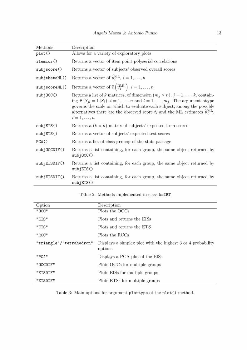
Methods Description
plot() Allows for a variety of exploratory plots
itemcor() Returns a vector of item point polyserial correlations
subjscore() Returns a vector of subjects’ observed overall scores
subjthetaML() Returns a vector of ϑMLi , i = 1, . . . , n
subjscoreML() Returns a vector of e(ϑMLi
), i = 1, . . . , n
subjOCC() Returns a list of k matrices, of dimension (mj × n), j = 1, . . . , k, contain-ing P (Yjl = 1 |Si ), i = 1, . . . , n and l = 1, . . . ,mj . The argument stype
governs the scale on which to evaluate each subject; among the possiblealternatives there are the observed score ti and the ML estimates ϑML
i ,i = 1, . . . , n
subjEIS() Returns a (k × n) matrix of subjects’ expected item scores
subjETS() Returns a vector of subjects’ expected test scores
PCA() Returns a list of class prcomp of the stats package
subjOCCDIF() Returns a list containing, for each group, the same object returned bysubjOCC()
subjEISDIF() Returns a list containing, for each group, the same object returned bysubjEIS()
subjETSDIF() Returns a list containing, for each group, the same object returned bysubjETS()
Table 2: Methods implemented in class ksIRT
Option Description
"OCC" Plots the OCCs
"EIS" Plots and returns the EISs
"ETS" Plots and returns the ETS
"RCC" Plots the RCCs
"triangle"/"tetrahedron" Displays a simplex plot with the highest 3 or 4 probabilityoptions
"PCA" Displays a PCA plot of the EISs
"OCCDIF" Plots OCCs for multiple groups
"EISDIF" Plots EISs for multiple groups
"ETSDIF" Plots ETSs for multiple groups
Table 3: Main options for argument plottype of the plot() method.

14 KernSmoothIRT: An R Package for Kernel Smoothing in Item Response Theory
Option characteristic curves
The code
R> plot(Psych1, plottype="OCC", item=c(24,25,92,96))
produces the OCCs for items 24, 25, 92, and 96 displayed in Figure 2. The correct options are
30 40 50 60 70 80 90
0.0
0.2
0.4
0.6
0.8
1.0
Item: 24
Expected Score
Pro
babi
lity
2
1
3
4
5% 25% 50% 75% 95%
(a) Item 24
30 40 50 60 70 80 90
0.0
0.2
0.4
0.6
0.8
1.0
Item: 25
Expected Score
Pro
babi
lity
1
3
4
NA
2
5% 25% 50% 75% 95%
(b) Item 25
30 40 50 60 70 80 90
0.0
0.2
0.4
0.6
0.8
1.0
Item: 92
Expected Score
Pro
babi
lity
2
31
4
5% 25% 50% 75% 95%
(c) Item 92
30 40 50 60 70 80 90
0.0
0.2
0.4
0.6
0.8
1.0
Item: 96
Expected Score
Pro
babi
lity
4
2
31
NA
5% 25% 50% 75% 95%
(d) Item 96
Figure 2: OCCs for items 24, 25, 92, and 96 of the introductory psychology exam.
displayed in blue and the incorrect options in red. The default specification axistype="scores"
uses the expected total score (9) as display variable on the x-axis. The vertical dashed lines
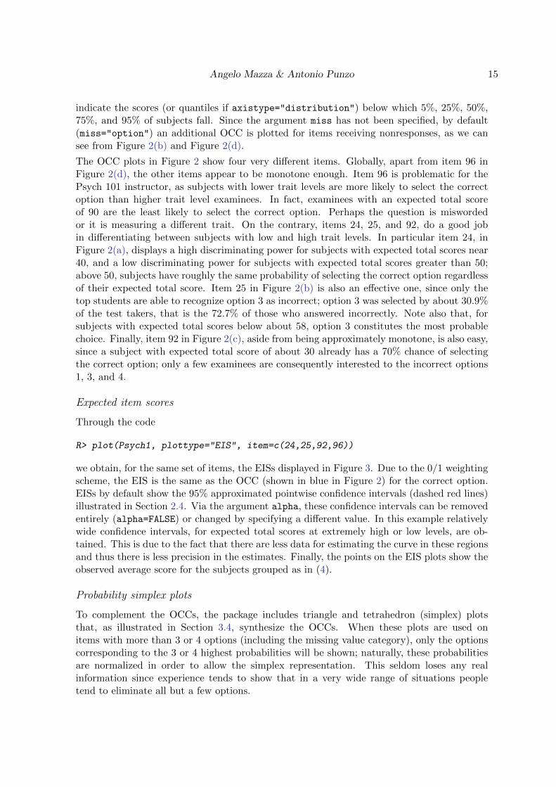
Angelo Mazza & Antonio Punzo 15
indicate the scores (or quantiles if axistype="distribution") below which 5%, 25%, 50%,75%, and 95% of subjects fall. Since the argument miss has not been specified, by default(miss="option") an additional OCC is plotted for items receiving nonresponses, as we cansee from Figure 2(b) and Figure 2(d).
The OCC plots in Figure 2 show four very different items. Globally, apart from item 96 inFigure 2(d), the other items appear to be monotone enough. Item 96 is problematic for thePsych 101 instructor, as subjects with lower trait levels are more likely to select the correctoption than higher trait level examinees. In fact, examinees with an expected total scoreof 90 are the least likely to select the correct option. Perhaps the question is miswordedor it is measuring a different trait. On the contrary, items 24, 25, and 92, do a good jobin differentiating between subjects with low and high trait levels. In particular item 24, inFigure 2(a), displays a high discriminating power for subjects with expected total scores near40, and a low discriminating power for subjects with expected total scores greater than 50;above 50, subjects have roughly the same probability of selecting the correct option regardlessof their expected total score. Item 25 in Figure 2(b) is also an effective one, since only thetop students are able to recognize option 3 as incorrect; option 3 was selected by about 30.9%of the test takers, that is the 72.7% of those who answered incorrectly. Note also that, forsubjects with expected total scores below about 58, option 3 constitutes the most probablechoice. Finally, item 92 in Figure 2(c), aside from being approximately monotone, is also easy,since a subject with expected total score of about 30 already has a 70% chance of selectingthe correct option; only a few examinees are consequently interested to the incorrect options1, 3, and 4.
Expected item scores
Through the code
R> plot(Psych1, plottype="EIS", item=c(24,25,92,96))
we obtain, for the same set of items, the EISs displayed in Figure 3. Due to the 0/1 weightingscheme, the EIS is the same as the OCC (shown in blue in Figure 2) for the correct option.EISs by default show the 95% approximated pointwise confidence intervals (dashed red lines)illustrated in Section 2.4. Via the argument alpha, these confidence intervals can be removedentirely (alpha=FALSE) or changed by specifying a different value. In this example relativelywide confidence intervals, for expected total scores at extremely high or low levels, are ob-tained. This is due to the fact that there are less data for estimating the curve in these regionsand thus there is less precision in the estimates. Finally, the points on the EIS plots show theobserved average score for the subjects grouped as in (4).
Probability simplex plots
To complement the OCCs, the package includes triangle and tetrahedron (simplex) plotsthat, as illustrated in Section 3.4, synthesize the OCCs. When these plots are used onitems with more than 3 or 4 options (including the missing value category), only the optionscorresponding to the 3 or 4 highest probabilities will be shown; naturally, these probabilitiesare normalized in order to allow the simplex representation. This seldom loses any realinformation since experience tends to show that in a very wide range of situations peopletend to eliminate all but a few options.
16 KernSmoothIRT: An R Package for Kernel Smoothing in Item Response Theory
30 40 50 60 70 80 90
0.0
0.2
0.4
0.6
0.8
1.0
Item: 24
Expected Score
Exp
ecte
d Ite
m S
core
●
●
● ●
●
●
● ●
●
●
●
● ●
●
●
●
●
●
●●
●
●
●
●
●
●
● ●
●●
●
●
●
●
● ● ●
●
● ● ● ● ● ● ● ● ● ●
5% 25% 50% 75% 95%
(a) Item 24
30 40 50 60 70 80 90
0.0
0.2
0.4
0.6
0.8
1.0
Item: 25
Expected Score
Exp
ecte
d Ite
m S
core
● ● ● ● ● ● ● ●
●
●
●
●
●
●
●
●
●
●
●
●
●
●
●
●
●
●
●
●
●
●
●
●
●
●
●
●
●
●
● ● ●
●
● ● ● ● ● ●
5% 25% 50% 75% 95%
(b) Item 25
30 40 50 60 70 80 90
0.0
0.2
0.4
0.6
0.8
1.0
Item: 92
Expected Score
Exp
ecte
d Ite
m S
core
●
●
● ●
●
●
●
●
●
● ●
●
●
●
●
●
●
●
●
● ●
●
● ● ● ● ●
● ● ● ●
●
●
●
● ● ●
●
● ● ● ● ● ● ● ● ● ●
5% 25% 50% 75% 95%
(c) Item 92
30 40 50 60 70 80 90
0.0
0.2
0.4
0.6
0.8
1.0
Item: 96
Expected Score
Exp
ecte
d Ite
m S
core
●
● ● ● ● ● ●
●
●
● ●
●
●
●
●
●
●
●
●
●
●
●
●
●
●
●
●
●
●
●
●
●
●
●
●
●
●
●
●
●
●
●
●
● ●
●
● ●
5% 25% 50% 75% 95%
(d) Item 96
Figure 3: EISs, and corresponding 95% pointwise confidence intervals (dashed red lines), foritems 24, 25, 92, and 96 of the introductory psychology exam. Grouped subject scores aredisplayed as points.
The tetrahedron is the natural choice for the items 24 and 92, characterized by four optionsand without “observed” missing responses; for these items the code
R> plot(Psych1, plottype="tetrahedron", items=c(24,92))
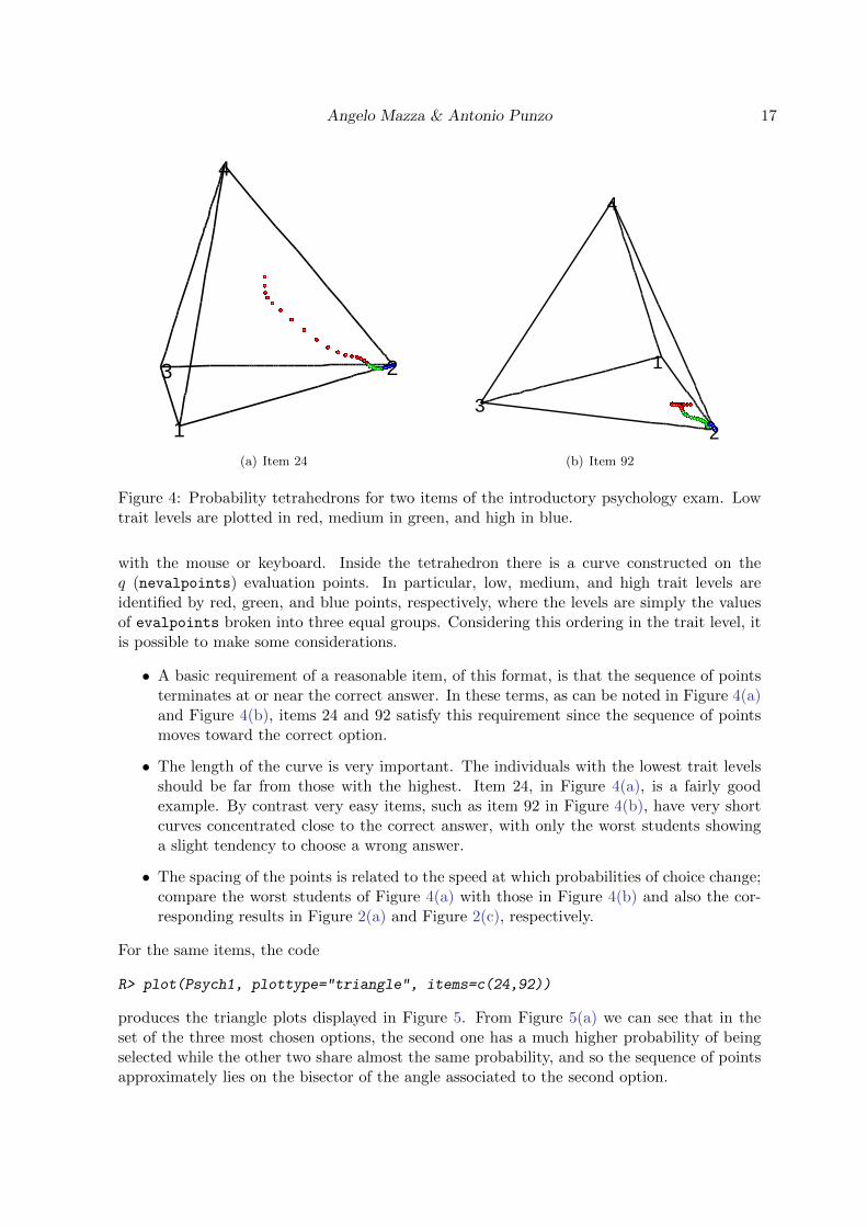
generates the tetrahedron plots displayed in Figure 2. These plots may be manipulated
Angelo Mazza & Antonio Punzo 17
3
1
Item : 24
4
2
(a) Item 24
Item : 92
1
4
2
3
(b) Item 92
Figure 4: Probability tetrahedrons for two items of the introductory psychology exam. Lowtrait levels are plotted in red, medium in green, and high in blue.
with the mouse or keyboard. Inside the tetrahedron there is a curve constructed on theq (nevalpoints) evaluation points. In particular, low, medium, and high trait levels areidentified by red, green, and blue points, respectively, where the levels are simply the valuesof evalpoints broken into three equal groups. Considering this ordering in the trait level, itis possible to make some considerations.
• A basic requirement of a reasonable item, of this format, is that the sequence of pointsterminates at or near the correct answer. In these terms, as can be noted in Figure 4(a)and Figure 4(b), items 24 and 92 satisfy this requirement since the sequence of pointsmoves toward the correct option.
• The length of the curve is very important. The individuals with the lowest trait levelsshould be far from those with the highest. Item 24, in Figure 4(a), is a fairly goodexample. By contrast very easy items, such as item 92 in Figure 4(b), have very shortcurves concentrated close to the correct answer, with only the worst students showinga slight tendency to choose a wrong answer.
• The spacing of the points is related to the speed at which probabilities of choice change;compare the worst students of Figure 4(a) with those in Figure 4(b) and also the cor-responding results in Figure 2(a) and Figure 2(c), respectively.
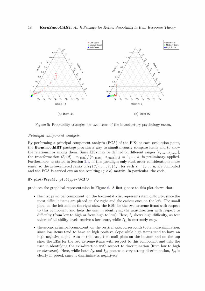
For the same items, the code
R> plot(Psych1, plottype="triangle", items=c(24,92))
produces the triangle plots displayed in Figure 5. From Figure 5(a) we can see that in theset of the three most chosen options, the second one has a much higher probability of beingselected while the other two share almost the same probability, and so the sequence of pointsapproximately lies on the bisector of the angle associated to the second option.
18 KernSmoothIRT: An R Package for Kernel Smoothing in Item Response Theory
Item : 24
Opt
ion
# :
4
0.1
0.2
0.3
0.4
0.5
0.6
0.7
0.8
0.9
Option # : 3
0.1
0.2
0.3
0.4
0.5
0.6
0.7
0.8
0.9
0.9
0.8
0.7
0.6
0.5
0.4
0.3
0.2
0.1
Option # : 2
●●●●●●●●●●●●●●●●●
●
Low ScoreMedium ScoreHigh Score
(a) Item 24
Item : 92
O
ptio
n #
: 1
0.1
0.2
0.3
0.4
0.5
0.6
0.7
0.8
0.9 O
ption # : 3
0.1
0.2
0.3
0.4
0.5
0.6
0.7
0.8
0.9
0.9
0.8
0.7
0.6
0.5
0.4
0.3
0.2
0.1
Option # : 2
●●●●●●●●●●●●●●●●●
●
Low ScoreMedium ScoreHigh Score
(b) Item 92
Figure 5: Probability triangles for two items of the introductory psychology exam.
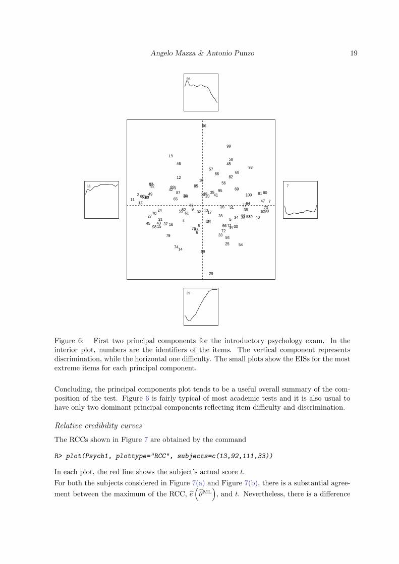
Principal component analysis
By performing a principal component analysis (PCA) of the EISs at each evaluation point,the KernsmoothIRT package provides a way to simultaneously compare items and to showthe relationships among them. Since EISs may be defined on different ranges [xjmin, xjmax],the transformation (ej (ϑ)− xjmin) / (xjmax − xjmin), j = 1, . . . , k, is preliminary applied.Furthermore, as stated in Section 2.1, in this paradigm only rank order considerations makesense, so the zero-centered ranks of e1 (ϑs) , . . . , ek (ϑs), for each s = 1, . . . , q, are computedand the PCA is carried out on the resulting (q × k)-matrix. In particular, the code
R> plot(Psych1, plottype="PCA")
produces the graphical representation in Figure 6. A first glance to this plot shows that:
• the first principal component, on the horizontal axis, represents item difficulty, since themost difficult items are placed on the right and the easiest ones on the left. The smallplots on the left and on the right show the EISs for the two extreme items with respectto this component and help the user in identifying the axis-direction with respect todifficulty (from low to high or from high to low). Here, I7 shows high difficulty, as testtakers of all ability levels receive a low score, while I11 is extremely easy.
• the second principal component, on the vertical axis, corresponds to item discrimination,since low items tend to have an high positive slope while high items tend to have anhigh negative slope. Also in this case, the small plots on the bottom and on the topshow the EISs for the two extreme items with respect to this component and help theuser in identifying the axis-direction with respect to discrimination (from low to highor viceversa). Here, while both I96 and I29 possess a very strong discrimination, I96 isclearly ill-posed, since it discriminates negatively.
Angelo Mazza & Antonio Punzo 19
1
2
3
4 5
6
7
8
9
1011
12
13
14
15 16
17
18
19
20
21
22
23
24
25
26
27 28
29
30
31
32
33
34
35
36
37
38
39 40
4142
43
44
45
46
47
48
49
50
5152
53
54
55
56
57
58
59
60
61 62
63
6465
66
67
68
69
70
7172
73
74
75
76
7778
79
8081
82
83
84
85
86
87
88
89
90
91
92
93
9495
96
9798
99
100
11 7
29
96
Figure 6: First two principal components for the introductory psychology exam. In theinterior plot, numbers are the identifiers of the items. The vertical component representsdiscrimination, while the horizontal one difficulty. The small plots show the EISs for the mostextreme items for each principal component.
Concluding, the principal components plot tends to be a useful overall summary of the com-position of the test. Figure 6 is fairly typical of most academic tests and it is also usual tohave only two dominant principal components reflecting item difficulty and discrimination.
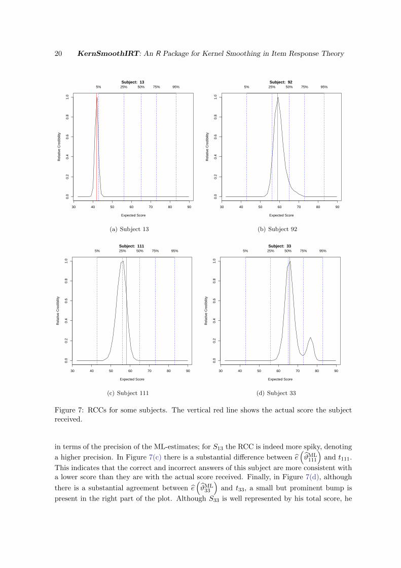
Relative credibility curves
The RCCs shown in Figure 7 are obtained by the command
R> plot(Psych1, plottype="RCC", subjects=c(13,92,111,33))
In each plot, the red line shows the subject’s actual score t.
For both the subjects considered in Figure 7(a) and Figure 7(b), there is a substantial agree-
ment between the maximum of the RCC, e(ϑML
), and t. Nevertheless, there is a difference
20 KernSmoothIRT: An R Package for Kernel Smoothing in Item Response Theory
30 40 50 60 70 80 90
0.0
0.2
0.4
0.6
0.8
1.0
Subject: 13
Expected Score
Rel
ativ
e C
redi
bilit
y
5% 25% 50% 75% 95%
(a) Subject 13
30 40 50 60 70 80 90
0.0
0.2
0.4
0.6
0.8
1.0
Subject: 92
Expected Score
Rel
ativ
e C
redi
bilit
y
5% 25% 50% 75% 95%
(b) Subject 92
30 40 50 60 70 80 90
0.0
0.2
0.4
0.6
0.8
1.0
Subject: 111
Expected Score
Rel
ativ
e C
redi
bilit
y
5% 25% 50% 75% 95%
(c) Subject 111
30 40 50 60 70 80 90
0.0
0.2
0.4
0.6
0.8
1.0
Subject: 33
Expected Score
Rel
ativ
e C
redi
bilit
y
5% 25% 50% 75% 95%
(d) Subject 33
Figure 7: RCCs for some subjects. The vertical red line shows the actual score the subjectreceived.
in terms of the precision of the ML-estimates; for S13 the RCC is indeed more spiky, denoting
a higher precision. In Figure 7(c) there is a substantial difference between e(ϑML111
)and t111.
This indicates that the correct and incorrect answers of this subject are more consistent witha lower score than they are with the actual score received. Finally, in Figure 7(d), although
there is a substantial agreement between e(ϑML33
)and t33, a small but prominent bump is
present in the right part of the plot. Although S33 is well represented by his total score, he
Angelo Mazza & Antonio Punzo 21
passed some, albeit few, difficult items and this may lead to think that he is more able thant33 suggests.
The commands
R> subjscore(Psych1)
[1] 74 56 89 70 56 57 ...
R> subjscoreML(Psych1)
[1] 72.36589 59.06626 88.47615 67.47167 57.71787 55.03844 ...
allow us to evaluate the differences between the values of ti and e(ϑMLi
), i = 1, . . . , n.
Test summary plots
The KernSmoothIRT package also contains many analytical tools to assess the test overall.Figure 8 shows a few of these, obtained via the code
R> plot(Psych1, plottype="expected")
R> plot(Psych1, plottype="sd")
R> plot(Psych1, plottype="density")
−3 −2 −1 0 1 2 3
3040
5060
7080
90
Expected Total Score
Norm 0 1 Quantiles
Exp
ecte
d S
core
5% 25% 50% 75% 95%
(a) Expected Test Score
30 40 50 60 70 80 90
2.5
3.0
3.5
4.0
4.5
Test Standard Deviation
Expected Score
Sta
ndar
d D
evia
tions
5% 25% 50% 75% 95%
(b) Standard Deviation
0 20 40 60 80
0.00
00.
005
0.01
00.
015
0.02
00.
025
0.03
0
Observed Score Distribution
Observed Scores
Den
sity
of S
core
5% 25% 50% 75% 95%
(c) Density
Figure 8: Test summary plots for the introductory psychology exam.
Figure 8(a) shows the ETS as a function of the quantiles of the standard normal distributionΦ; it is nearly linear for the Psych 101 dataset. Note that, in the nonparametric context, theETS may be non-monotone due to either ill-posed items or random variations. In the lattercase, a slight increase of the bandwidth may be advisable.
The total score, for subjects having a particular value ϑ, is a random variable, in part becausedifferent examinees, or even the same examinee on different occasions, cannot be expectedto make exactly the same choices. The standard deviation of these values, graphically repre-sented in Figure 8(b), is therefore also a function of ϑ. Figure 8(b) indicates that the standarddeviation reaches the maximum for examinees at around a total score of 50, where it is about

22 KernSmoothIRT: An R Package for Kernel Smoothing in Item Response Theory
4.5 items out of 100. This translates into 95% confidence limits of about 41 and 59 for asubject getting 50 items correct.
Figure 8(c) shows a kernel density estimate of the distribution of the total score. Althoughsuch distribution is commonly assumed to be “bell-shaped”, from this plot we can note as thisassumption is strong for these data. In particular, a negative skewness can be noted whichis a consequence of the test having relatively more easy items than hard ones. Moreover,bimodality is evident.
4.3. Voluntary HIV-1 counseling and testing efficacy study group
It is often useful to explore if, for a specific item on a test, its expected score differs when esti-mated on two or more different groups of subjects, commonly formed by gender or ethnicity.This is called Differential Item Functioning (DIF) analysis in the psychometric literature. Inparticular, DIF occurs when subjects with the same ability but belonging to different groupshave a different probability of choosing a certain option. DIF can properly be called itembias because the curves of an item should depend only on ϑ, and not directly on other personfactors. Zumbo (2007) offers a recent review of various DIF detection methods and strategies.
The KernSmoothIRT package allows for a nonparametric graphical analysis of DIF, based onkernel smoothing methods. To illustrate this analysis, we use data coming from the Volun-tary HIV Counseling and Testing Efficacy Study, conducted in 1995-1997 by the Center forAIDS Prevention Studies at University of California, San Francisco (see The Voluntary HIV-1Counseling and Testing Efficacy Study Group 2000a,b, for details). This study was concernedwith the effectiveness of HIV counseling and testing in reducing risk behavior for the sexualtransmission of HIV. To perform this study, n = 4292 persons were enrolled. The wholedataset – downloadable from http://caps.ucsf.edu/research/datasets/, which also con-tains other useful survey details – reported 1571 variables for each participant. As part ofthis study, respondents were surveyed about their attitude toward condom use via a bank ofk = 15 items. Respondents were asked how much they agreed with each of the statements on a4-point response scale, with 1=“strongly disagree”, 2=“disagree more than I agree”, 3=“agreemore than I disagree”, 4=“strongly agree”). Since 10 individuals omitted all the 15 questions,they have been preliminary removed from the used data. Moreover, given the (“negative”)wording of the items I2, I3, I5, I7, I8, I11, and I14, a respondent who strongly agreed with suchstatements was indicating a less favorable attitude toward condom use. In order to uniformthe data, the score for these seven items was preliminary reversed. The dataset so modifiedcan be directly loaded from the KernSmoothIRT package by the code
R> data("HIV")
R> HIV
SITE GENDER AGE 1 2 3 4 5 6 7 8 9 10 11 12 13 14 15
1 Ken F 17 4 1 1 4 1 2 4 4 4 4 3 4 1 2 4
2 Ken F 17 4 2 4 4 2 3 1 4 3 3 2 3 4 1 4
3 Ken F 18 4 4 4 4 4 1 4 4 4 1 NA 4 1 NA 4
. . . . . . . . . . . . . . . . . . .
. . . . . . . . . . . . . . . . . . .
. . . . . . . . . . . . . . . . . . .
Angelo Mazza & Antonio Punzo 23
4281 Tri M 79 4 4 1 4 1 NA 4 NA 4 NA NA NA NA 1 4
4282 Tri M 80 4 NA 4 4 1 4 NA NA NA 1 NA 4 1 4 NA
R> attach(HIV)
As it can be easily seen, the above data frame contains the following person factors:
SITE = “site of the study” (Ken=Kenya, Tan=Tanzania, Tri=Trinidad)GENDER = “subject’s gender” (M=male, F=female)
AGE = “subject’s age” (age at last birthday)
Each of these factors can potentially be used for a DIF analysis. These data have been alsoanalyzed, through some well-known parametric models, by Bertoli-Barsotti, Muschitiello, andPunzo (2010) which also perform a DIF analysis. Part of this sub-questionnaire has been alsoconsidered by De Ayala (2003, 2009) with a Rasch Analysis.
The code below
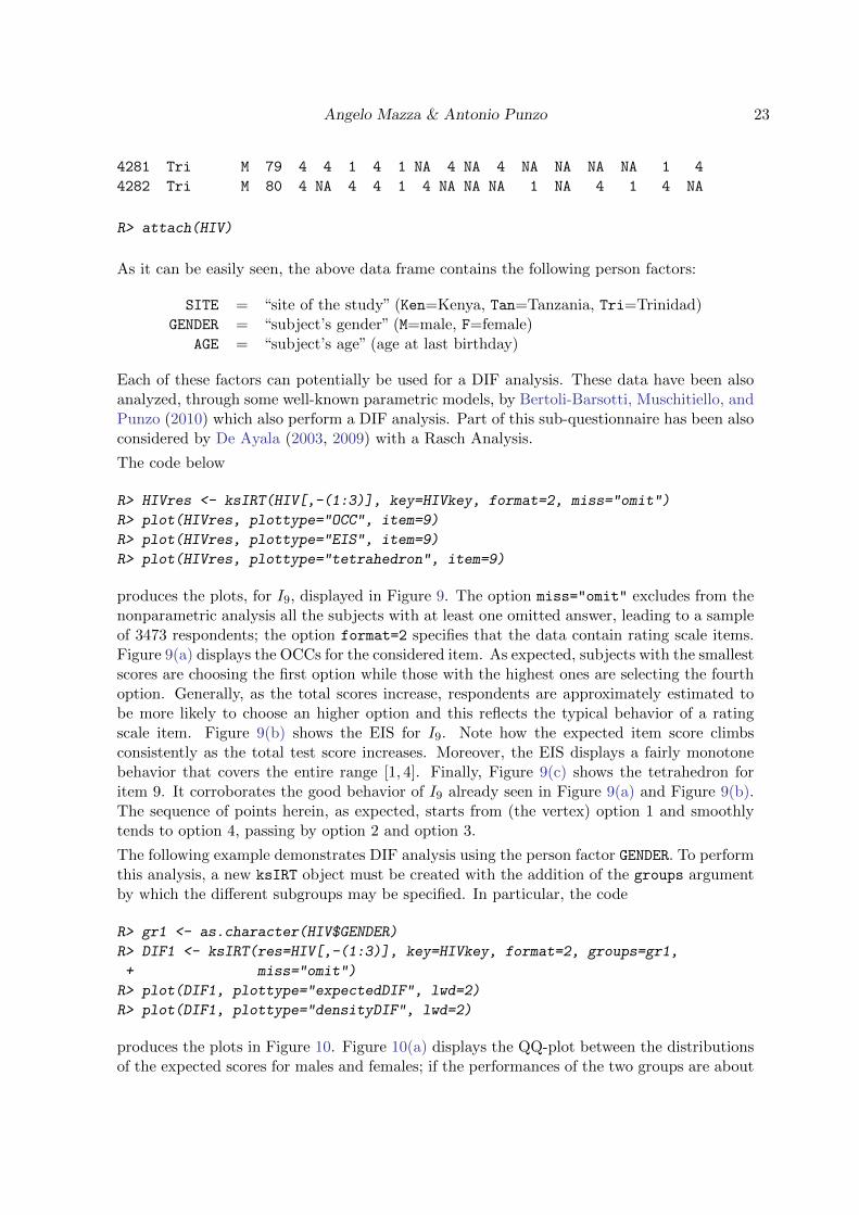
R> HIVres <- ksIRT(HIV[,-(1:3)], key=HIVkey, format=2, miss="omit")
R> plot(HIVres, plottype="OCC", item=9)
R> plot(HIVres, plottype="EIS", item=9)
R> plot(HIVres, plottype="tetrahedron", item=9)
produces the plots, for I9, displayed in Figure 9. The option miss="omit" excludes from thenonparametric analysis all the subjects with at least one omitted answer, leading to a sampleof 3473 respondents; the option format=2 specifies that the data contain rating scale items.Figure 9(a) displays the OCCs for the considered item. As expected, subjects with the smallestscores are choosing the first option while those with the highest ones are selecting the fourthoption. Generally, as the total scores increase, respondents are approximately estimated tobe more likely to choose an higher option and this reflects the typical behavior of a ratingscale item. Figure 9(b) shows the EIS for I9. Note how the expected item score climbsconsistently as the total test score increases. Moreover, the EIS displays a fairly monotonebehavior that covers the entire range [1, 4]. Finally, Figure 9(c) shows the tetrahedron foritem 9. It corroborates the good behavior of I9 already seen in Figure 9(a) and Figure 9(b).The sequence of points herein, as expected, starts from (the vertex) option 1 and smoothlytends to option 4, passing by option 2 and option 3.
The following example demonstrates DIF analysis using the person factor GENDER. To performthis analysis, a new ksIRT object must be created with the addition of the groups argumentby which the different subgroups may be specified. In particular, the code
R> gr1 <- as.character(HIV$GENDER)
R> DIF1 <- ksIRT(res=HIV[,-(1:3)], key=HIVkey, format=2, groups=gr1,
+ miss="omit")
R> plot(DIF1, plottype="expectedDIF", lwd=2)
R> plot(DIF1, plottype="densityDIF", lwd=2)
produces the plots in Figure 10. Figure 10(a) displays the QQ-plot between the distributionsof the expected scores for males and females; if the performances of the two groups are about
24 KernSmoothIRT: An R Package for Kernel Smoothing in Item Response Theory
20 30 40 50 60
0.0
0.2
0.4
0.6
0.8
1.0
Item: 9
Expected Score
Pro
babi
lity
4
3
1
2
5% 25% 50% 75% 95%
(a) OCCs
20 30 40 50 60
1.0
1.5
2.0
2.5
3.0
3.5
4.0
Item: 9
Expected Score
Exp
ecte
d Ite
m S
core
● ● ● ●
●
●
●
●
●●
●
●
●
●
●
●
●
●
●
●
●
●
●
● ●
●
●
●
●
●●
●
●
●
●
●
●
●
●
●
●
●●
● ● ●●●●●
5% 25% 50% 75% 95%
(b) EIS
3
4
2
Item : 9
1
(c) Tetrahedron
Figure 9: Item 9 from the voluntary HIV-1 counseling and testing efficacy study group.
the same, the relationship will appear as a nearly diagonal line (a dotted diagonal line isplotted as a reference). Figure 10(b) shows the density functions for the two groups. Bothplots confirm that there is a strong agreement in behavior for males and females with respectto the test.
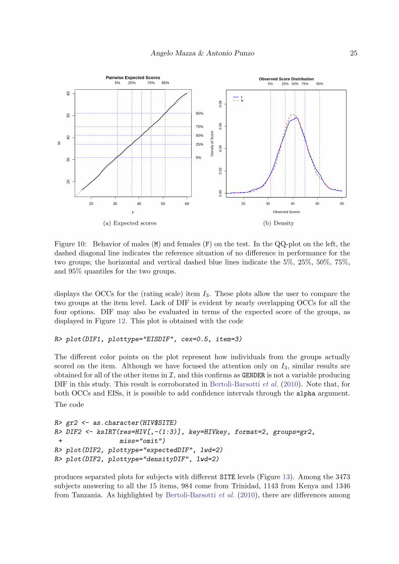
After this preliminary phase, the DIF analysis proceeds by considering the item by item groupcomparisons. Figure 11, obtained via the command
R> plot(DIF1, plottype="OCCDIF", cex=0.5, item=3)
Angelo Mazza & Antonio Punzo 25
20 30 40 50 60
2030
4050
60
Pairwise Expected Scores
F
M
5% 25% 75% 95%
5%
25%
50%
75%
95%
(a) Expected scores
20 30 40 50 60
0.00
0.02
0.04
0.06
0.08
Observed Score Distribution
Observed ScoresD
ensi
ty o
f Sco
re
FM
5% 25% 50% 75% 95%
(b) Density
Figure 10: Behavior of males (M) and females (F) on the test. In the QQ-plot on the left, thedashed diagonal line indicates the reference situation of no difference in performance for thetwo groups; the horizontal and vertical dashed blue lines indicate the 5%, 25%, 50%, 75%,and 95% quantiles for the two groups.
displays the OCCs for the (rating scale) item I3. These plots allow the user to compare thetwo groups at the item level. Lack of DIF is evident by nearly overlapping OCCs for all thefour options. DIF may also be evaluated in terms of the expected score of the groups, asdisplayed in Figure 12. This plot is obtained with the code
R> plot(DIF1, plottype="EISDIF", cex=0.5, item=3)
The different color points on the plot represent how individuals from the groups actuallyscored on the item. Although we have focused the attention only on I3, similar results areobtained for all of the other items in I, and this confirms as GENDER is not a variable producingDIF in this study. This result is corroborated in Bertoli-Barsotti et al. (2010). Note that, forboth OCCs and EISs, it is possible to add confidence intervals through the alpha argument.
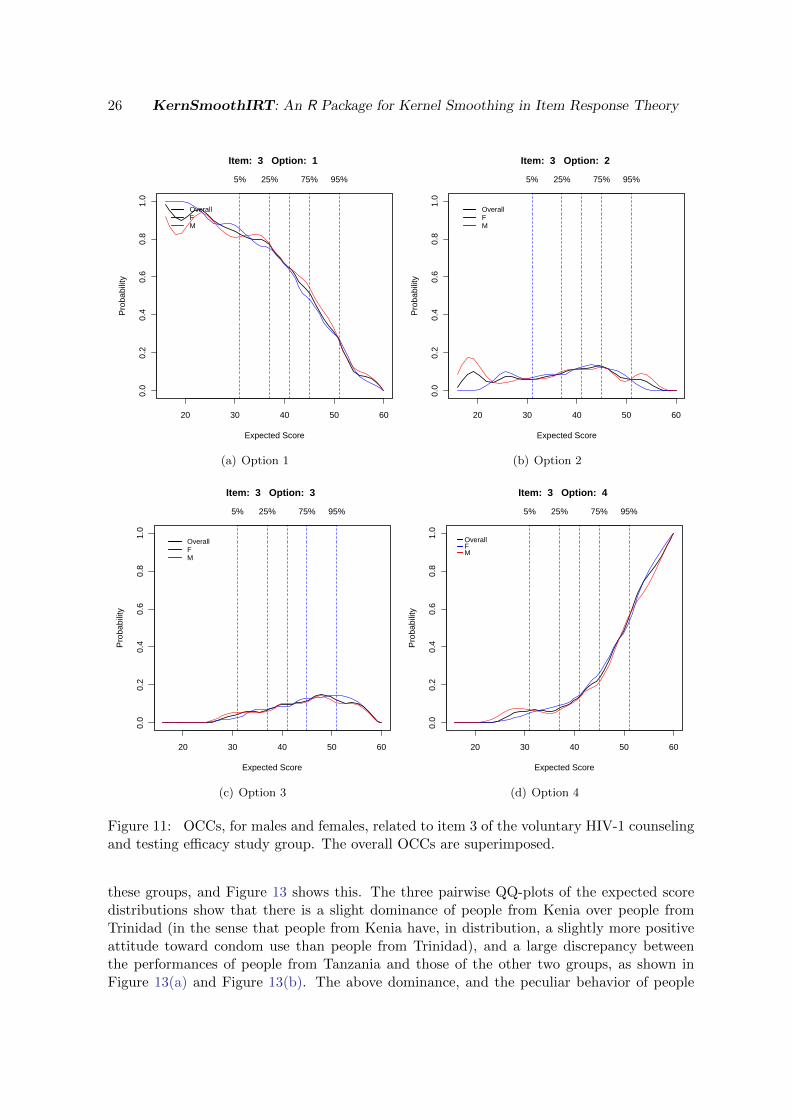
The code
R> gr2 <- as.character(HIV$SITE)
R> DIF2 <- ksIRT(res=HIV[,-(1:3)], key=HIVkey, format=2, groups=gr2,
+ miss="omit")
R> plot(DIF2, plottype="expectedDIF", lwd=2)
R> plot(DIF2, plottype="densityDIF", lwd=2)
produces separated plots for subjects with different SITE levels (Figure 13). Among the 3473subjects answering to all the 15 items, 984 come from Trinidad, 1143 from Kenya and 1346from Tanzania. As highlighted by Bertoli-Barsotti et al. (2010), there are differences among
26 KernSmoothIRT: An R Package for Kernel Smoothing in Item Response Theory
20 30 40 50 60
0.0
0.2
0.4
0.6
0.8
1.0
Item: 3 Option: 1
Expected Score
Pro
babi
lity
5% 25% 75% 95%
OverallFM
(a) Option 1
20 30 40 50 60
0.0
0.2
0.4
0.6
0.8
1.0
Item: 3 Option: 2
Expected Score
Pro
babi
lity
5% 25% 75% 95%
OverallFM
(b) Option 2
20 30 40 50 60
0.0
0.2
0.4
0.6
0.8
1.0
Item: 3 Option: 3
Expected Score
Pro
babi
lity
5% 25% 75% 95%
OverallFM
(c) Option 3
20 30 40 50 60
0.0
0.2
0.4
0.6
0.8
1.0
Item: 3 Option: 4
Expected Score
Pro
babi
lity
5% 25% 75% 95%
OverallFM
(d) Option 4
Figure 11: OCCs, for males and females, related to item 3 of the voluntary HIV-1 counselingand testing efficacy study group. The overall OCCs are superimposed.
these groups, and Figure 13 shows this. The three pairwise QQ-plots of the expected scoredistributions show that there is a slight dominance of people from Kenia over people fromTrinidad (in the sense that people from Kenia have, in distribution, a slightly more positiveattitude toward condom use than people from Trinidad), and a large discrepancy betweenthe performances of people from Tanzania and those of the other two groups, as shown inFigure 13(a) and Figure 13(b). The above dominance, and the peculiar behavior of people
Angelo Mazza & Antonio Punzo 27
20 30 40 50 60
1.0
1.5
2.0
2.5
3.0
3.5
4.0
Item: 3
Expected Score
Exp
ecte
d Ite
m S
core
● ● ● ● ● ● ●
●
●
●
●
●
●
●
●
●
●
● ●
●
●●
●
●●
●
●
●
●
●
●●
●
●
●
●
●
●
●
●
●
●
● ● ●●●●
● ● ●
●
● ● ●
●
●
●
●
● ●
●
●
●● ●
●
●
●
● ●
●
●
●
●
●
●
●●
●
●
●
●
●
●
●
●
●
●
●
● ● ●●●●
5% 25% 50% 75% 95%
OverallFM
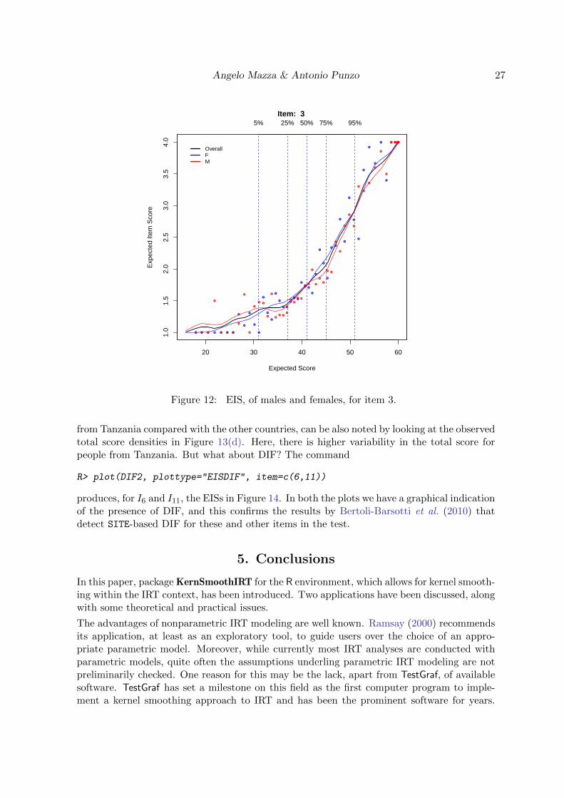
Figure 12: EIS, of males and females, for item 3.
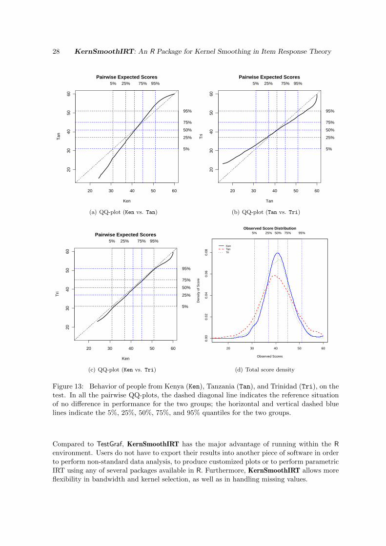
from Tanzania compared with the other countries, can be also noted by looking at the observedtotal score densities in Figure 13(d). Here, there is higher variability in the total score forpeople from Tanzania. But what about DIF? The command
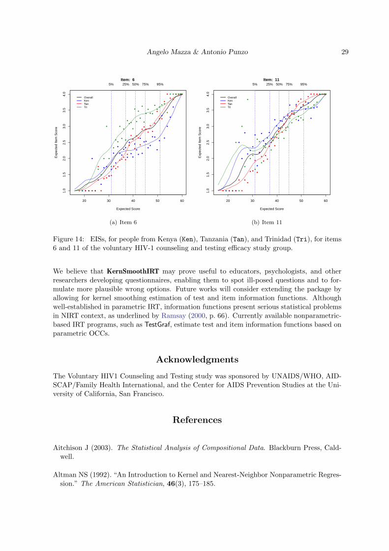
R> plot(DIF2, plottype="EISDIF", item=c(6,11))
produces, for I6 and I11, the EISs in Figure 14. In both the plots we have a graphical indicationof the presence of DIF, and this confirms the results by Bertoli-Barsotti et al. (2010) thatdetect SITE-based DIF for these and other items in the test.
5. Conclusions
In this paper, package KernSmoothIRT for the R environment, which allows for kernel smooth-ing within the IRT context, has been introduced. Two applications have been discussed, alongwith some theoretical and practical issues.
The advantages of nonparametric IRT modeling are well known. Ramsay (2000) recommendsits application, at least as an exploratory tool, to guide users over the choice of an appro-priate parametric model. Moreover, while currently most IRT analyses are conducted withparametric models, quite often the assumptions underling parametric IRT modeling are notpreliminarily checked. One reason for this may be the lack, apart from TestGraf, of availablesoftware. TestGraf has set a milestone on this field as the first computer program to imple-ment a kernel smoothing approach to IRT and has been the prominent software for years.
28 KernSmoothIRT: An R Package for Kernel Smoothing in Item Response Theory
20 30 40 50 60
2030
4050
60
Pairwise Expected Scores
Ken
Tan
5% 25% 75% 95%
5%
25%
50%
75%
95%
(a) QQ-plot (Ken vs. Tan)
20 30 40 50 60
2030
4050
60
Pairwise Expected Scores
TanT
ri
5% 25% 75% 95%
5%
25%
50%
75%
95%
(b) QQ-plot (Tan vs. Tri)
20 30 40 50 60
2030
4050
60
Pairwise Expected Scores
Ken
Tri
5% 25% 75% 95%
5%
25%
50%
75%
95%
(c) QQ-plot (Ken vs. Tri)
20 30 40 50 60
0.00
0.02
0.04
0.06
0.08
Observed Score Distribution
Observed Scores
Den
sity
of S
core
KenTanTri
5% 25% 50% 75% 95%
(d) Total score density
Figure 13: Behavior of people from Kenya (Ken), Tanzania (Tan), and Trinidad (Tri), on thetest. In all the pairwise QQ-plots, the dashed diagonal line indicates the reference situationof no difference in performance for the two groups; the horizontal and vertical dashed bluelines indicate the 5%, 25%, 50%, 75%, and 95% quantiles for the two groups.
Compared to TestGraf, KernSmoothIRT has the major advantage of running within the Renvironment. Users do not have to export their results into another piece of software in orderto perform non-standard data analysis, to produce customized plots or to perform parametricIRT using any of several packages available in R. Furthermore, KernSmoothIRT allows moreflexibility in bandwidth and kernel selection, as well as in handling missing values.
Angelo Mazza & Antonio Punzo 29
20 30 40 50 60
1.0
1.5
2.0
2.5
3.0
3.5
4.0
Item: 6
Expected Score
Exp
ecte
d Ite
m S
core
● ● ●
●
●
●
●
●
●
●
●
●
●
●
●
●
●
●
●
●
●
●
●
●
●
●
●
●●
●
●
● ●
●
●
●
●
●
●
●
● ● ● ●●●
● ● ● ● ●
●
●
●●
● ●
●
●
●
●●
●
●
●
●
●
●
●
●
●
●
●
●
●
●
●
●
●
●
● ●
●
●
●
●
● ● ● ●●●
● ● ● ●
●
●
●
●
●
●
●
●
●
●
●
●
●
●
●
●
●
●
●
●
●
●
●
●
●
●●
●
●
●
●
●
●
● ● ● ● ● ●●
5% 25% 50% 75% 95%
OverallKenTanTri
(a) Item 6
20 30 40 50 60
1.0
1.5
2.0
2.5
3.0
3.5
4.0
Item: 11
Expected Score
Exp
ecte
d Ite
m S
core
● ● ● ●
●
●
●
●
●
●
●
●
●
●
●
●
●
●
●
●
●
●
●
●●
●
●
●
●
●
●
●
●
●
●
●
●
●
●●
● ● ● ●●●
● ● ● ●
●
●
●
●
●●
●
●
●
●
●
●
●
●
●
●
●
●
●
●
●
●
●
●
●
●●
●
●
●
●
●
●
● ● ● ● ● ● ●●●
● ●
●
●
●
●
●
●
●
●
●
●
●
●
●
●
●
●
●
●
●
●
●
●
●
●
●
●
●
●
●
●
●
●
●
●●
●
●
● ● ● ●●
5% 25% 50% 75% 95%
OverallKenTanTri
(b) Item 11
Figure 14: EISs, for people from Kenya (Ken), Tanzania (Tan), and Trinidad (Tri), for items6 and 11 of the voluntary HIV-1 counseling and testing efficacy study group.
We believe that KernSmoothIRT may prove useful to educators, psychologists, and otherresearchers developing questionnaires, enabling them to spot ill-posed questions and to for-mulate more plausible wrong options. Future works will consider extending the package byallowing for kernel smoothing estimation of test and item information functions. Althoughwell-established in parametric IRT, information functions present serious statistical problemsin NIRT context, as underlined by Ramsay (2000, p. 66). Currently available nonparametric-based IRT programs, such as TestGraf, estimate test and item information functions based onparametric OCCs.
Acknowledgments
The Voluntary HIV1 Counseling and Testing study was sponsored by UNAIDS/WHO, AID-SCAP/Family Health International, and the Center for AIDS Prevention Studies at the Uni-versity of California, San Francisco.
References
Aitchison J (2003). The Statistical Analysis of Compositional Data. Blackburn Press, Cald-well.
Altman NS (1992). “An Introduction to Kernel and Nearest-Neighbor Nonparametric Regres-sion.” The American Statistician, 46(3), 175–185.
30 KernSmoothIRT: An R Package for Kernel Smoothing in Item Response Theory
Azzalini A, Bowman AW, Hardle W (1989). “On the Use of Nonparametric Regression forModel Checking.” Biometrika, 76(1), 1–11.
Baker FB, Kim SH (2004). Item Response Theory: Parameter Estimation Techniques. Statis-tics: A Dekker Series of Textbooks and Monographs. Marcel Dekker, New York.
Bartholomew DJ (1983). “Latent Variable Models for Ordered Categorical Data.” Journal ofEconometrics, 22(1–2), 229–243.
Bartholomew DJ (1988). “The Sensitivity of Latent Trait Analysis to Choice of Prior Distri-bution.” British Journal of Mathematical and Statistical Psychology, 41(1), 101–107.
Bertoli-Barsotti L, Muschitiello C, Punzo A (2010). “Item Analysis of a Selected Bank fromthe Voluntary HIV-1 Counseling and Testing Efficacy Study Group.” Technical Report 1,Dipartimento di Matematica, Statistica, Informatica e Applicazioni (Lorenzo Mascheroni),Universita degli Studi di Bergamo. URL http://aisberg.unibg.it/bitstream/10446/
444/1/WPMateRi01(2010).pdf.
Chang HH, Mazzeo J (1994). “The Unique Correspondence of the Item Response Functionand Item Category Response Functions in Polytomously Scored Item Response Models.”Psychometrika, 59(3), 391–404.
De Ayala RJ (2003). “The Effect of Missing Data on Estimating a Respondent’s LocationUsing Ratings Data.” Journal of Applied Measurement, 4(1), 1–9.
De Ayala RJ (2009). The Theory and Practice of Item Response Theory. Methodology in theSocial Sciences. Guilford Press, New York.
de Leeuw J, Mair P (2007). “An Introduction to the Special Volume on “Psychometrics in R”.”Journal of Statistical Software, 20(1), 1–5. URL http://www.jstatsoft.org/v20/i01.
DeMars C (2010). Item Response Theory. Understanding Statistics. Oxford University Press,New York.
Douglas JA (1997). “Joint Consistency of Nonparametric Item Characteristic Curve andAbility Estimation.” Psychometrika, 62(1), 7–28.
Douglas JA (2001). “Asymptotic Identifiability of Nonparametric Item Response Models.”Psychometrika, 66(4), 531–540.
Douglas JA, Cohen A (2001). “Nonparametric Item Response Function Estimation for As-sessing Parametric Model Fit.” Applied Psychological Measurement, 25(3), 234–243.
Guttman L (1947). “The Cornell Technique for Scale and Intensity Analysis.” Educationaland Psychological Measurement, 7(2), 247–279.
Guttman L (1950a). “Relation of scalogram analysis to other techniques.” In SA Stouf-fer, L Guttman, FA Suchman, PF Lazarsfeld, SA Star, JA Clausen (eds.), Measurementand Prediction, volume 4 of Studies in Social Psychology in World War II, pp. 172–212.Princeton University Press, Princeton, NJ.

Angelo Mazza & Antonio Punzo 31
Guttman LA (1950b). “The Basis for Scalogram Analysis.” In SA Stouffer, L Guttman,FA Suchman, PF Lazarsfeld, SA Star, JA Clausen (eds.), Measurement and Prediction,volume 4 of Studies in Social Psychology in World War II, pp. 60–90. Princeton UniversityPress, Princeton, NJ.
Hardle W (1990). Applied Nonparametric Regression, volume 19 of Econometric SocietyMonographs. Cambridge University Press, Cambridge.
Junker BW, Sijtsma K (2001). “Nonparametric Item Response Theory in Action: AnOverview of the Special Issue.” Applied Psychological Measurement, 25(3), 211–220.
Kutylowski AJ (1997). “Nonparametric Latent Factor Analysis of Occupational InventoryData.” In J Rost, R Langeheine (eds.), Applications of Latent Trait and Latent ClassModels in the Social Sciences, pp. 253–266. Vaxmann, New York.
Lei PW, Dunbar SB, Kolen MJ (2004). “A Comparison of Parametric and Non-ParametricApproaches to Item Analysis for Multiple-Choice Tests.” Educational and PsychologicalMeasurement, 64(3), 1–23.
Lindsey JK (1973). Inferences from Sociological Survey Data: A Unified Approach, volume 3of Progress in Mathematical Social Sciences. Elsevier Scientific Publishing Company, Am-sterdam.
Lord FM (1980). Application of Item Response Theory to Practical Testing Problems.Lawrence Erlbaum Associates, Hillsdale.
Marron JS, Nolan D (1988). “Canonical Kernels for Density Estimation.” Statistics & Prob-ability Letters, 7(3), 195–199.
Mazza A, Punzo A (2011). “Discrete Beta Kernel Graduation of Age-Specific DemographicIndicators.” In S Ingrassia, R Rocci, M Vichi (eds.), New Perspectives in Statistical Modelingand Data Analysis, Studies in Classification, Data Analysis, and Knowledge Organization,pp. 127–134. Springer-Verlag, Berlin Heidelberg.
Mazza A, Punzo A (2013a). “Graduation by Adaptive Discrete Beta Kernels.” In A Giusti,G Ritter, M Vichi (eds.), Classification and Data Mining, Studies in Classification, DataAnalysis, and Knowledge Organization, pp. 243–250. Springer-Verlag, Berlin Heidelberg.
Mazza A, Punzo A (2013b). “Using the Variation Coefficient for Adaptive Discrete BetaKernel Graduation.” In P Giudici, S Ingrassia, M Vichi (eds.), Statistical Models for DataAnalysis, Studies in Classification, Data Analysis, and Knowledge Organization, pp. 225–232. Springer International Publishing, Switzerland.
Mazza A, Punzo A (2014). “DBKGrad: An R Package for Mortality Rates Graduation byDiscrete Beta Kernel Techniques.” Journal of Statistical Software, 57(Code Snippet 2),1–18.
Mokken RJ (1971). A Theory and Procedure of Scale Analysis, volume 1 of Methods andModels in the Social Sciences. The Gruyter, Berlin, Germany.
Nadaraya EA (1964). “On Estimating Regression.” Theory of Probability and Its Applications,9(1), 141–142.
32 KernSmoothIRT: An R Package for Kernel Smoothing in Item Response Theory
Nering ML, Ostini R (2010). Handbook of Polytomous Item Response Theory Models. Taylor& Francis, New York.
Olsson U, Drasgow F, Dorans NJ (1982). “The Polyserial Correlation Coefficient.” Psychome-trika, 47(3), 337–347.
Ostini R, Nering ML (2006). Polytomous Item Response Theory Models, volume 144 ofQuantitative Applications in the Social Sciences. SAGE, London.
R Core Team (2013). R: A Language and Environment for Statistical Computing. R Founda-tion for Statistical Computing, Vienna, Austria. URL http://www.R-project.org.
Punzo A (2009). “On Kernel Smoothing in Polytomous IRT: A New Minimum DistanceEstimator.” Quaderni di Statistica, 11, 15–37.
Ramsay JO (1991). “Kernel Smoothing Approaches to Nonparametric Item CharacteristicCurve Estimation.” Psychometrika, 56(4), 611–630.
Ramsay JO (1997). “A Functional Approach to Modeling Test Data.” In WJ van der Linden,RK Hambleton (eds.), Handbook of Modern Item Response Theory, pp. 381–394. Springer,New York.
Ramsay JO (2000). TestGraf: A Program for the Graphical Analysis of Multiple Choice Testand Questionnaire Data. URL http://www.psych.mcgill.ca/faculty/ramsay/ramsay.
html.
Ramsay JO, Abrahamowicz M (1989). “Binomial Regression with Monotone Splines: APsychometric Application.” Journal of the American Statistical Association, 84(408), 906–915.
Rice J (1984). “Bandwidth Choice for Nonparametric Regression.” The Annals of Statistics,12(4), 1215–1230.
Silverman BW (1986). Density Estimation for Statistics and Data Analysis, volume 26 ofMonographs on Statistics & Applied Probability. Chapman & Hall, London.
Simonoff JS (1996). Smoothing Methods in Statistics. Springer Series in Statistics. Springer,New York.
The Voluntary HIV-1 Counseling and Testing Efficacy Study Group (2000a). “Efficacy ofVoluntary HIV-1 Counseling and Testing in Individual and Couples in Kenya, Tanzania,and Trinidad: A Randomised Trial.” Lancet, 356(9224), 103–112.
The Voluntary HIV-1 Counseling and Testing Efficacy Study Group (2000b). “The VoluntaryHIV-1 Counseling and Testing Efficacy Study: Design and Methods.” AIDS and Behavior,4(1), 5–14.
Thissen D, Steinberg L (1986). “A Taxonomy of Item Response Models.” Psychometrika,51(4), 567–577.
van der Ark LA (2001). “Relationships and Properties of Polytomous Item Response Models.”Applied Psychological Measurement, 25(3), 273–282.

Angelo Mazza & Antonio Punzo 33
van der Ark LA (2007). “Mokken Scale Analysis in R.” Journal of Statistical Software, 20(11),1–19. URL http://www.jstatsoft.org/v20/i11.
van der Linden WJ, Hambleton RK (1997). Handbook of Modern Item Response Theory.Springer, New York.
Watson GS (1964). “Smooth Regression Analysis.” Sankhy Aitclose, Series A, 26(4), 359–372.
Wickelmaier F, Strobl C, Zeileis A (2012). “Psychoco: Psychometric Computing in R.” Journalof Statistical Software, 48(1), 1–5. URL http://www.jstatsoft.org/v48/i01.
Wong WH (1983). “On the Consistency of Cross-Validation in Kernel Nonparametric Regres-sion.” The Annals of Statistics, 11(4), 1136–1141.
Zumbo BD (2007). “Three Generations of Differential Item Functioning (DIF) Analyses:Considering Where It Has Been, Where It Is Now, and Where It Is Going.” LanguageAssessment Quarterly, 4(2), 223–233.
Affiliation:
Angelo Mazza, Antonio PunzoDepartment of Economics and BusinessUniversity of CataniaCorso Italia, 55, 95129 Catania, ItalyE-mail: [email protected], [email protected]: http://www.economia.unict.it/a.mazza, http://www.economia.unict.it/punzo
Brian McGuireDepartment of StatisticsMontana State UniversityBozeman, Montana, USAE-mail: [email protected]