kangwook kim and waymond r. scott, jr
TRANSCRIPT

Sensor and Simulation Notes
Note 481
31 October 2003
Analysis of Impulse-Radiating Antennaswith Ellipsoidal Reflectors
Kangwook Kim and Waymond R. Scott, Jr.
School of Electrical and Computer Engineering
Georgia Institute of Technology
ABSTRACT
An IRA can effectively focus its radiation in the near field by using an ellipsoidalreflector. In this paper, three IRAs with ellipsoidal reflectors (elliptic IRAs) are numericallyanalyzed and compared with an IRA with a typical parabolic reflector (parabolic IRA). Theellipsoidal reflector is parameterized by the distance between the center of the reflector andits closest focus (F ), the distance between the two optical foci (Φ), and the diameter of thereflector (D). The IRAs have the same F/D, i.e., 0.5, but different Φ/D’s, i.e., 0.5, 1.0,and 1.5. The electric fields in the near-field region and the reflected voltage in the feedingtransmission line are analyzed. The elliptic IRAs have a larger impulse and a smaller beamin the near-field region than does the parabolic IRA. The maximum impulse amplitude andthe minimum beam width do not occur at the optical focus for the input pulse considered inthis paper. The amplitudes of the tail waveform and the reflected voltage in the transmissionline are increased.
I. Introduction
In a typical reflector-type impulse-radiating antenna (IRA), a spherical transverse
electromagnetic (TEM) wave is guided by TEM feed arms and converted into an equi-phase
aperture by a parabolic reflector [1–4]. The aperture is focused at infinity in the geometrical
optics sense, and the radiated waveform of the aperture at its optical focus is an impulse
when it is driven by a step pulse. Thus, the IRA with a parabolic reflector (parabolic IRA)
is capable of transmitting a temporally short pulse on boresight in the far-field region.
Recently, researchers have been considering IRAs for use in ground penetrating radar
(GPR) systems because of the short pulse radiation capability [5,6]. However, for most GPR
systems, the target is close to the antennas. In this region, the impulse part of the waveform
is not fully developed, so the performance of the IRA is degraded [7, 8].
In order to improve the performance of the IRA for this application, the aperture
must be focused at a distance close to the antenna. This can be achieved by using a portion
of an ellipsoid of revolution as a reflector [9]. An ellipsoid of revolution has two optical foci,
and an optics ray originating at one focus arrives at the other focus with the same amount
of delay after a single bounce at any point on the ellipsoid. Thus, the aperture formed by
the ellipsoidal reflector is focused on the second focus.
The characteristics of an IRA with an ellipsoidal reflector (elliptic IRA) over a wide
bandwidth may be understood by a numerical model. Thus, in this paper, we investigate
the characteristics of the elliptic IRAs by modeling the antennas numerically. The numerical
model is developed using the method of moments code in EIGER [10,11]. The performance
of the numerical model using EIGER has been validated in [8].
II. Modeling of the IRAs
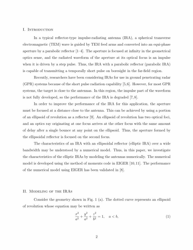
Consider the geometry shown in Fig. 1 (a). The dotted curve represents an ellipsoid
of revolution whose equation may be written as
x2
a2+
y2
a2+
z2
b2= 1, a < b, (1)
2
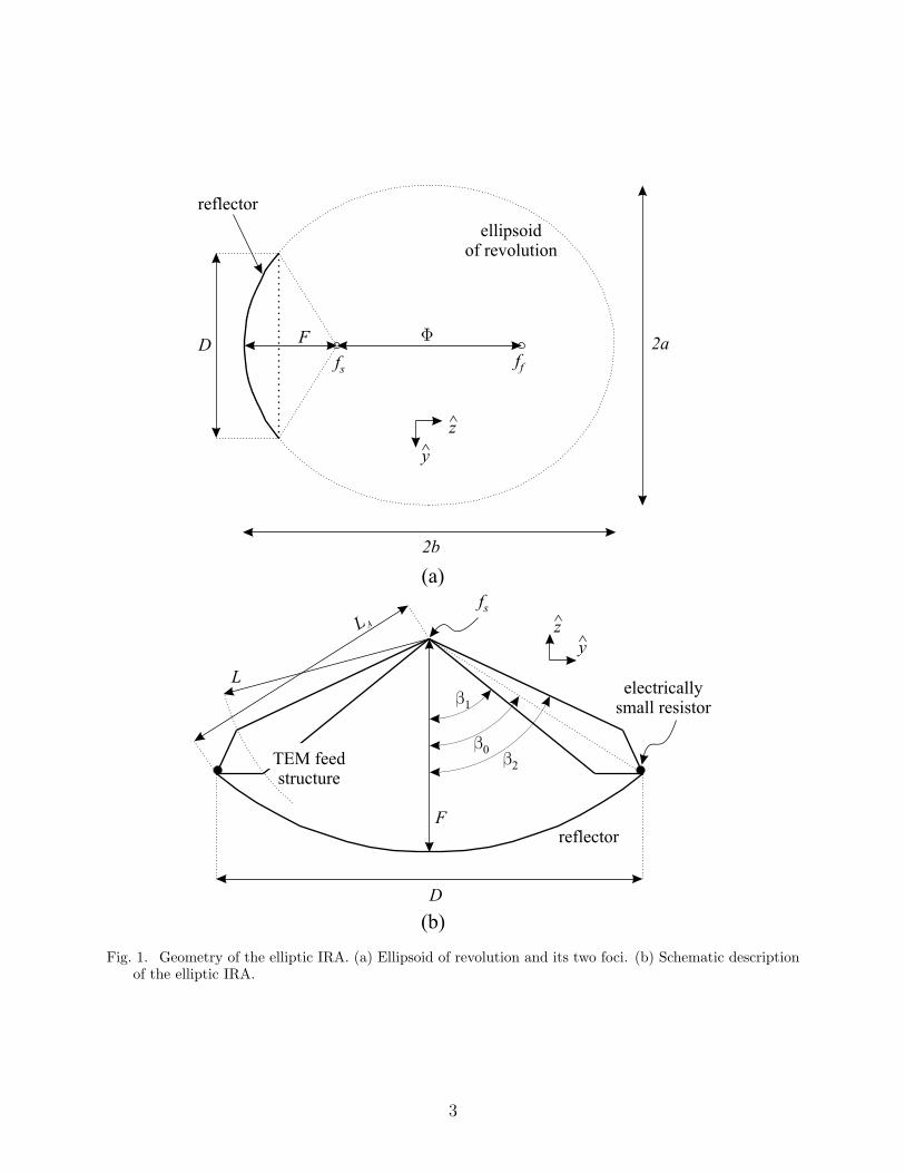
Fig. 1. Geometry of the elliptic IRA. (a) Ellipsoid of revolution and its two foci. (b) Schematic descriptionof the elliptic IRA.
3
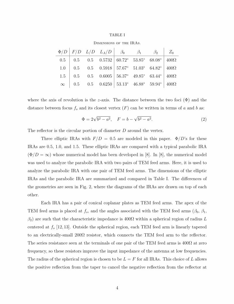
TABLE I
Dimensions of the IRAs.
Φ/D F/D L/D LA/D β0 β1 β2 Z0
0.5 0.5 0.5 0.5732 60.72 53.85 68.08 400Ω
1.0 0.5 0.5 0.5918 57.67 51.03 64.82 400Ω
1.5 0.5 0.5 0.6005 56.37 49.85 63.44 400Ω
∞ 0.5 0.5 0.6250 53.13 46.88 59.94 400Ω
where the axis of revolution is the z-axis. The distance between the two foci (Φ) and the
distance between focus fs and its closest vertex (F ) can be written in terms of a and b as:
Φ = 2√
b2 − a2, F = b−√
b2 − a2. (2)
The reflector is the circular portion of diameter D around the vertex.
Three elliptic IRAs with F/D = 0.5 are modeled in this paper. Φ/D’s for these
IRAs are 0.5, 1.0, and 1.5. These elliptic IRAs are compared with a typical parabolic IRA
(Φ/D = ∞) whose numerical model has been developed in [8]. In [8], the numerical model
was used to analyze the parabolic IRA with two pairs of TEM feed arms. Here, it is used to
analyze the parabolic IRA with one pair of TEM feed arms. The dimensions of the elliptic
IRAs and the parabolic IRA are summarized and compared in Table I. The differences of
the geometries are seen in Fig. 2, where the diagrams of the IRAs are drawn on top of each
other.
Each IRA has a pair of conical coplanar plates as TEM feed arms. The apex of the
TEM feed arms is placed at fs, and the angles associated with the TEM feed arms (β0, β1,
β2) are such that the characteristic impedance is 400Ω within a spherical region of radius L
centered at fs [12, 13]. Outside the spherical region, each TEM feed arm is linearly tapered
to an electrically-small 200Ω resistor, which connects the TEM feed arm to the reflector.
The series resistance seen at the terminals of one pair of the TEM feed arms is 400Ω at zero
frequency, so these resistors improve the input impedance of the antenna at low frequencies.
The radius of the spherical region is chosen to be L = F for all IRAs. This choice of L allows
the positive reflection from the taper to cancel the negative reflection from the reflector at
4
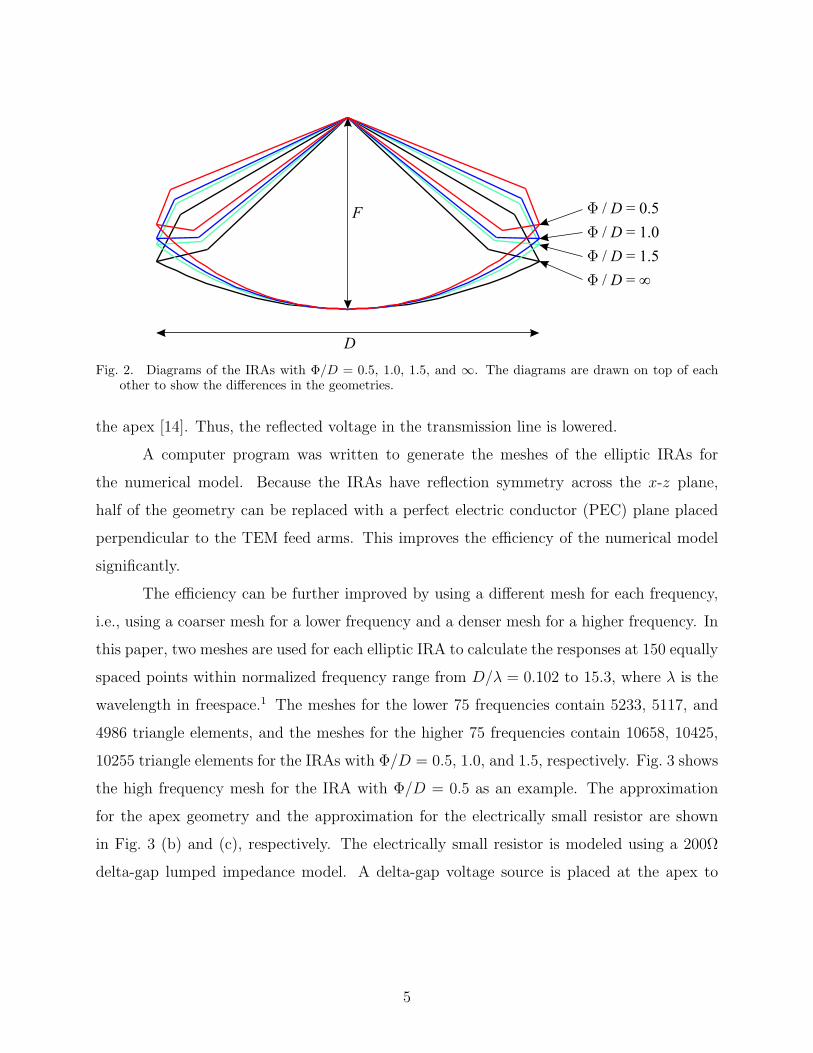
Fig. 2. Diagrams of the IRAs with Φ/D = 0.5, 1.0, 1.5, and ∞. The diagrams are drawn on top of eachother to show the differences in the geometries.
the apex [14]. Thus, the reflected voltage in the transmission line is lowered.
A computer program was written to generate the meshes of the elliptic IRAs for
the numerical model. Because the IRAs have reflection symmetry across the x-z plane,
half of the geometry can be replaced with a perfect electric conductor (PEC) plane placed
perpendicular to the TEM feed arms. This improves the efficiency of the numerical model
significantly.
The efficiency can be further improved by using a different mesh for each frequency,
i.e., using a coarser mesh for a lower frequency and a denser mesh for a higher frequency. In
this paper, two meshes are used for each elliptic IRA to calculate the responses at 150 equally
spaced points within normalized frequency range from D/λ = 0.102 to 15.3, where λ is the
wavelength in freespace.1 The meshes for the lower 75 frequencies contain 5233, 5117, and
4986 triangle elements, and the meshes for the higher 75 frequencies contain 10658, 10425,
10255 triangle elements for the IRAs with Φ/D = 0.5, 1.0, and 1.5, respectively. Fig. 3 shows
the high frequency mesh for the IRA with Φ/D = 0.5 as an example. The approximation
for the apex geometry and the approximation for the electrically small resistor are shown
in Fig. 3 (b) and (c), respectively. The electrically small resistor is modeled using a 200Ω
delta-gap lumped impedance model. A delta-gap voltage source is placed at the apex to
5
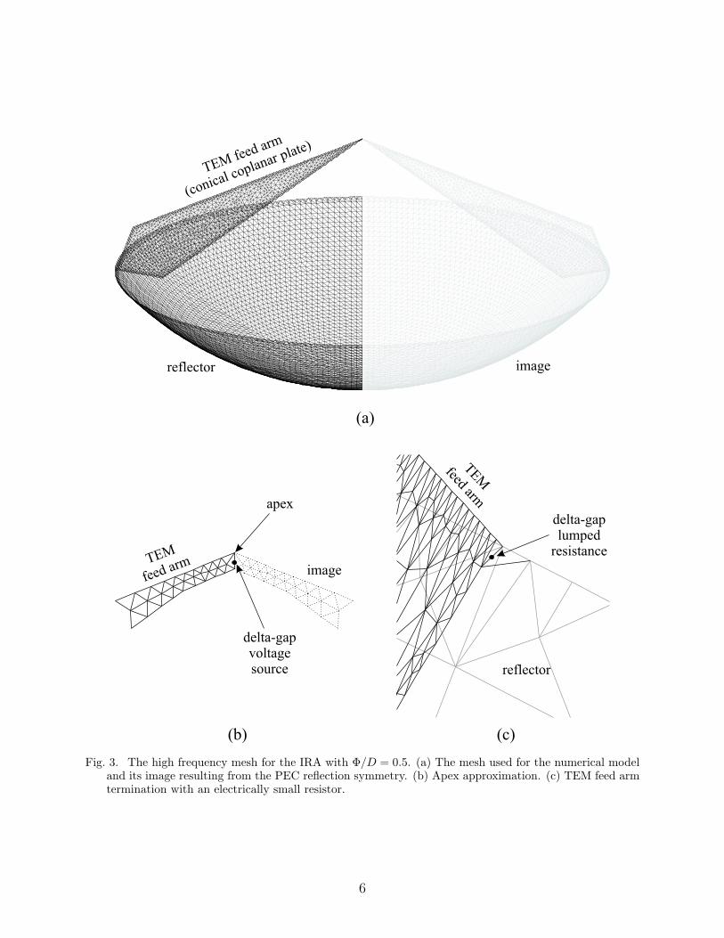
Fig. 3. The high frequency mesh for the IRA with Φ/D = 0.5. (a) The mesh used for the numerical modeland its image resulting from the PEC reflection symmetry. (b) Apex approximation. (c) TEM feed armtermination with an electrically small resistor.
6
excite the mesh.
The electric field integral equation with linear basis functions is used to solve for the
mesh currents. The EIGER physics solver (EIGER Solve) was executed in parallel on the
Beowulf cluster at the Electromagnetics/Acoustics Laboratory using the message passing
interface (MPI) protocol to produce the mesh currents. The run times were approximately
79.0, 72.3, 66.8 hours for the IRAs with Φ/D = 0.5, 1.0, and 1.5, respectively, using 32
computer nodes; each node is equipped with an AMD AthlonTM 2200+ processor. The
electric fields are obtained by running the EIGER physics solver for secondary quantities
(EIGER Analyze). The numerical results are valid for the half IRAs. The responses of the
full IRAs can be obtained by simple algebraic manipulations of the quantities generated by
the numerical model, i.e., doubling the input impedances and halving the currents and fields.
III. Analysis
In this paper, each antenna is fed by a transmission line, which has the same char-
acteristic impedance as the TEM feed arms. The responses in the frequency domain are
transformed into the time domain for input voltage pulses incident in the transmission line.
The input pulses considered in this paper are step-like and Gaussian pulses, which are defined
as follows:
Step-like: V (t) = V0
1
2+
1
2erf
(k1
t
t10-90%
), (3)
k1 = 2 erf−1(0.8) ' 1.8124,
Gaussian: V (t) = V0e− ln 16(t/tFWHM )2 , (4)
where erf(t) is the error function, V0 is the maximum amplitude of the pulse, and the pulse
parameters t10-90% and tFWHM are the 10% – 90% rise time of the step-like pulse and the
1Note that the upper frequency limit was chosen because of computer run time considerations, not limits on theIRA. The chosen upper frequency limit gives us reasonable run times while giving us enough frequency content tosee essentially all of the interesting interactions in the antennas. This upper frequency limit sets the minimum pulseparameters in the later graphs.
7

full-width half-maximum of the Gaussian pulse, respectively [15]. The waveforms and their
frequency spectrums are shown in [8].
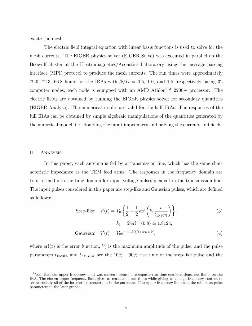
Fig. 4 shows electric fields of the antennas in the near-field region. In each graph, the
electric fields (Ey/V0) on the z-axis are plotted as a function of time for a step-like pulse
with t10-90%/τa = 0.075 and vertically displaced according to the observation distance. Here,
the parameter τa = D/c is the time required by light to travel the length of the reflector
diameter. For antennas with a finite Φ, the electric field at focus ff is plotted with a dotted
line.
The figure shows that the impulse is stronger for a smaller Φ in the near-field region.
The impulse of the antenna with a smaller Φ grows faster and also decays faster. These
are the expected results by focusing the aperture at distances close to the antenna. Note,
however, that the maximum impulse amplitude does not occur at focus ff because the
electrical size of the aperture is small compared to the ratio Φ/D. It has been empirically
found that for a square aperture of side length a, a/λ ≥ 25Φ/a is required to result in
the maximum amplitude close to focus ff [16]. For a circular aperture, this requirement is
approximatelyD
λ≥ 100
π
Φ
D. (5)
The minimum requirement corresponds to D/λ ≥ 15.9, 31.8, and 47.7 for the IRAs with
Φ/D = 0.5, 1.0, and 1.5, respectively. These requirements are all higher than the frequency
range we used in the numerical model (max D/λ = 15.3). The maximum impulse amplitude
will occur close to focus ff by using pulses with a faster rise time.
In Fig. 5, the envelope of the impulse amplitude (max Ey/V0) is plotted for each IRA
for step-like pulses with t10-90%/τa = 0.075 and 0.2. The envelopes with larger amplitudes
are those for t10-90%/τa = 0.075, and the envelopes with smaller amplitudes are those for
t10-90%/τa = 0.2. As noted in Fig. 4, the impulse envelope for the IRA with a smaller Φ
grows faster than the impulse envelope for the IRA with a larger Φ. It also decays faster
after it reaches its maximum. For example, for t10-90%/τa = 0.075, the impulse envelope for
the IRA with Φ/D = 0.5 grows faster and remains larger than those for other IRAs until
r/D ' 0.8. After it reaches its maximum at r/D ' 0.4, it decays faster and becomes smaller
8
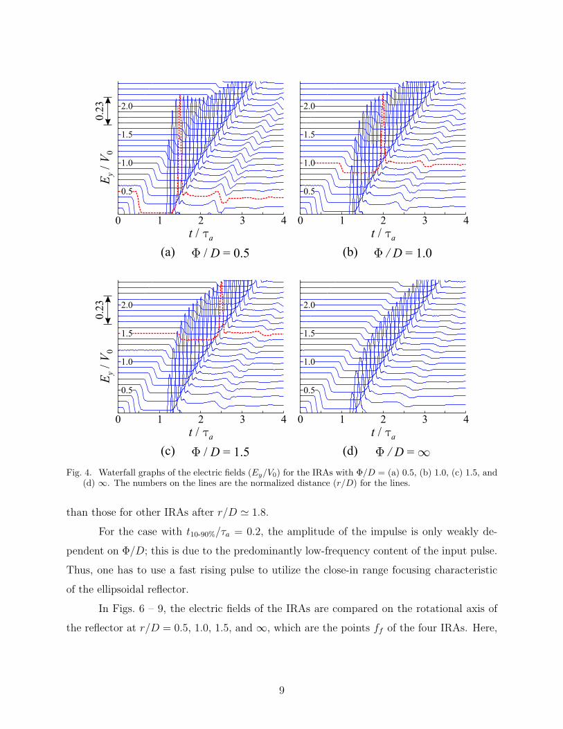
Fig. 4. Waterfall graphs of the electric fields (Ey/V0) for the IRAs with Φ/D = (a) 0.5, (b) 1.0, (c) 1.5, and(d) ∞. The numbers on the lines are the normalized distance (r/D) for the lines.
than those for other IRAs after r/D ' 1.8.
For the case with t10-90%/τa = 0.2, the amplitude of the impulse is only weakly de-
pendent on Φ/D; this is due to the predominantly low-frequency content of the input pulse.
Thus, one has to use a fast rising pulse to utilize the close-in range focusing characteristic
of the ellipsoidal reflector.
In Figs. 6 – 9, the electric fields of the IRAs are compared on the rotational axis of
the reflector at r/D = 0.5, 1.0, 1.5, and ∞, which are the points ff of the four IRAs. Here,
9
Fig. 5. Impulse envelopes (max Ey/V0) for step-like pulses with t10-90%/τa = 0.075 and 0.2.
the graphs are plotted for a step-like pulse with t10-90%/τa = 0.1 as functions of retarded
time tr = t− r/c, where r is the distance from the apex (fs) to the observer. In each figure,
the impulses are magnified in (b), and the prepulses and postpulses are magnified in (c).
At each observation distance, the impulse centered at tr/τa = 1.0 is the one from the
IRA with Φ equal to the observation distance (Φ = r). The impulse appears earlier than
tr/τa = 1.0 for the IRAs with Φ > r and later than tr/τa = 1.0 for the IRAs with Φ < r.
Because the IRA is focused at ff , the signal from any point on the reflector arrives at ff with
the same amount of time delay. At a point other than ff , the signals from different points
on the reflector arrive with different time delays. For example, for the IRA with Φ/D = 0.5,
the signal from each point on the reflector arrives at r/D = 0.5 at tr/τa = 1.0. Thus, the
peak occurs exactly at tr/τa = 1.0. However at r/D = 1.0, the signal from the center of
the reflector arrives at tr/τa = 1.0 while the signal from the edge of the reflector arrives at
tr/τa = 0.948. Thus, the peak occurs between tr/τa = 0.948 and tr/τa = 1.0.
One would think the amplitude of the impulse for the IRA with Φ = r should be
larger at r = Φ than those for the other IRAs because of the focusing; this is correct in
10
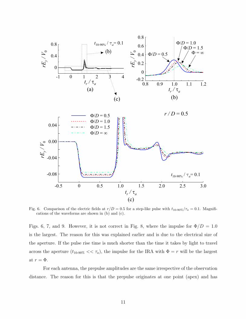
Fig. 6. Comparison of the electric fields at r/D = 0.5 for a step-like pulse with t10-90%/τa = 0.1. Magnifi-cations of the waveforms are shown in (b) and (c).
Figs. 6, 7, and 9. However, it is not correct in Fig. 8, where the impulse for Φ/D = 1.0
is the largest. The reason for this was explained earlier and is due to the electrical size of
the aperture. If the pulse rise time is much shorter than the time it takes by light to travel
across the aperture (t10-90% << τa), the impulse for the IRA with Φ = r will be the largest
at r = Φ.
For each antenna, the prepulse amplitudes are the same irrespective of the observation
distance. The reason for this is that the prepulse originates at one point (apex) and has
11

Fig. 7. Comparison of the electric fields at r/D = 1.0 for a step-like pulse with t10-90%/τa = 0.1. Magnifi-cations of the waveforms are shown in (b) and (c).
a 1/r dependence. Thus, the amplitude becomes constant when it is normalized by V0/r.
However, at any observation point, the prepulse for the IRA with a smaller Φ is larger than
that for the IRA with a larger Φ because the TEM feed arms are more inclined toward the
boresight direction guiding more energy toward the boresight direction.
The waveform at tr/τa ' 1.2 is due to the re-radiation of the signal taking the apex –
resistor – apex path. The waveform at tr/τa ' 2.0 is due to a number of internally reflected
signals, and it dominates the tail waveform. This waveform is larger for the IRA with a
12
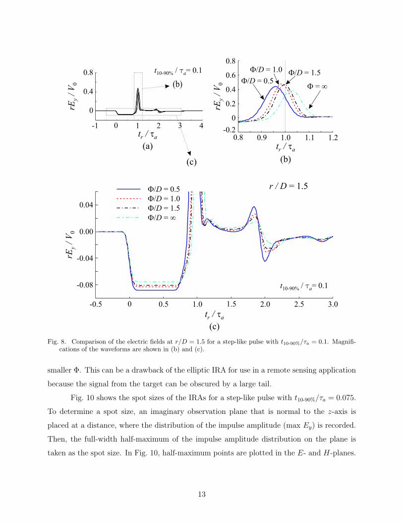
Fig. 8. Comparison of the electric fields at r/D = 1.5 for a step-like pulse with t10-90%/τa = 0.1. Magnifi-cations of the waveforms are shown in (b) and (c).
smaller Φ. This can be a drawback of the elliptic IRA for use in a remote sensing application
because the signal from the target can be obscured by a large tail.
Fig. 10 shows the spot sizes of the IRAs for a step-like pulse with t10-90%/τa = 0.075.
To determine a spot size, an imaginary observation plane that is normal to the z-axis is
placed at a distance, where the distribution of the impulse amplitude (max Ey) is recorded.
Then, the full-width half-maximum of the impulse amplitude distribution on the plane is
taken as the spot size. In Fig. 10, half-maximum points are plotted in the E- and H-planes.
13
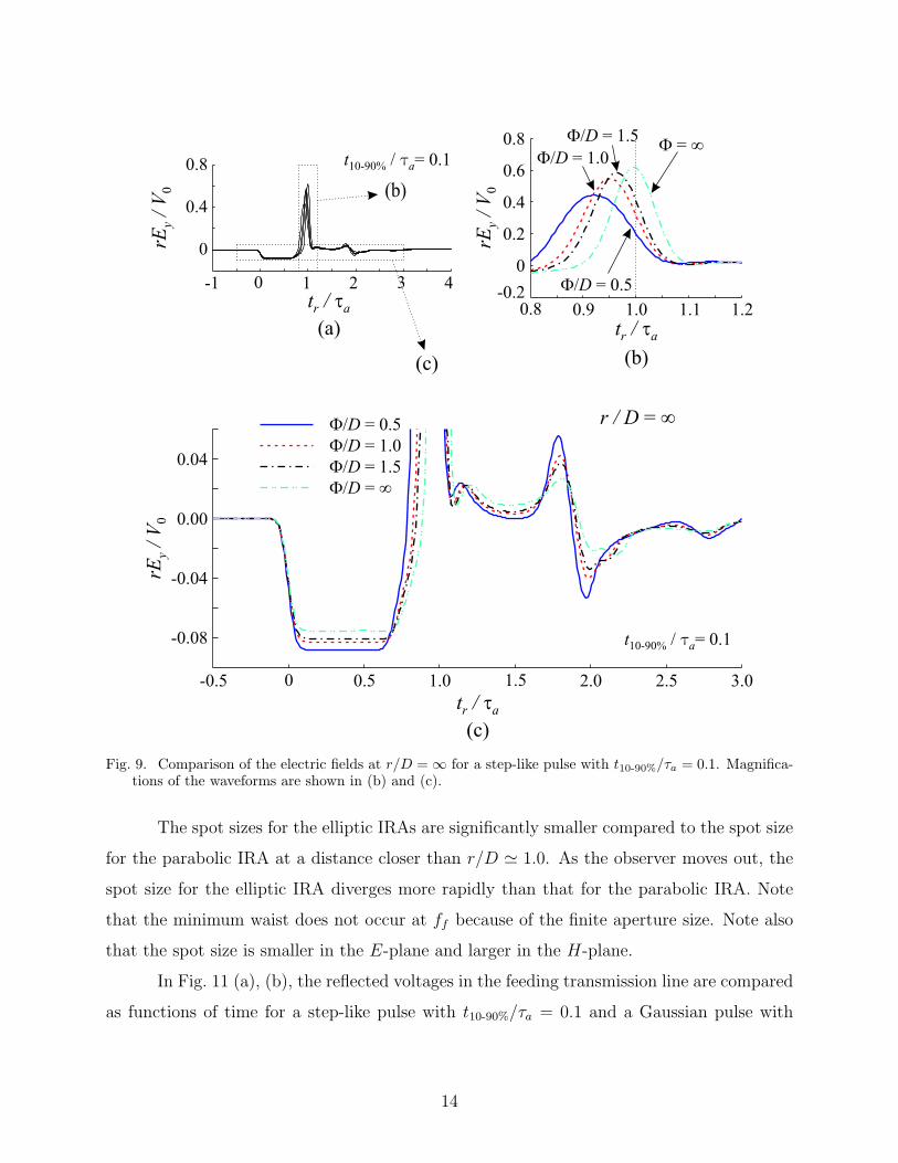
Fig. 9. Comparison of the electric fields at r/D = ∞ for a step-like pulse with t10-90%/τa = 0.1. Magnifica-tions of the waveforms are shown in (b) and (c).
The spot sizes for the elliptic IRAs are significantly smaller compared to the spot size
for the parabolic IRA at a distance closer than r/D ' 1.0. As the observer moves out, the
spot size for the elliptic IRA diverges more rapidly than that for the parabolic IRA. Note
that the minimum waist does not occur at ff because of the finite aperture size. Note also
that the spot size is smaller in the E-plane and larger in the H-plane.
In Fig. 11 (a), (b), the reflected voltages in the feeding transmission line are compared
as functions of time for a step-like pulse with t10-90%/τa = 0.1 and a Gaussian pulse with
14
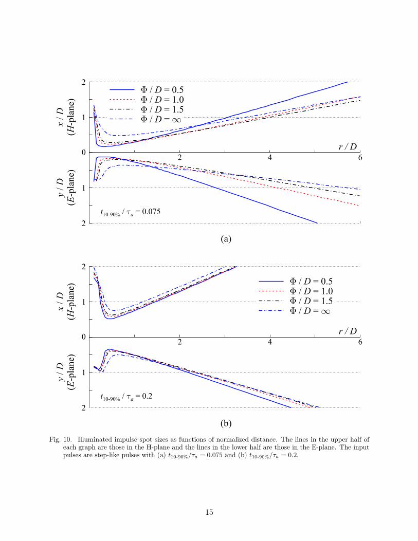
Fig. 10. Illuminated impulse spot sizes as functions of normalized distance. The lines in the upper half ofeach graph are those in the H-plane and the lines in the lower half are those in the E-plane. The inputpulses are step-like pulses with (a) t10-90%/τa = 0.075 and (b) t10-90%/τa = 0.2.
15
tFWHM/τa = 0.1. The magnifications of the waveforms surrounded by the boxes are shown
in Fig. 11 (c), (d). In Fig. 11 (a), (b), the first pulse around t/τa = 0 is the reflection from the
junction between the feeding transmission line and the antenna (fs). This reflection is due
to the approximation made to the apex geometry (Fig. 3 (b)). The first possible disturbance
after this reflection is the superposition of the positive signal from the TEM feed arm and
negative signal from the reflector; both signals begin at t/τa = 1.0. In Fig. 11 (a), the
waveform is not exactly zero over the time interval 0 < t/τa < 1.0 because of a small error
in the characteristic impedance of the TEM feed arms predicted by the numerical model
(∼ 1%).
The waveforms have the maximum amplitudes around t/τa = 1.2. The maximum
amplitude increases with decreasing Φ. Because the reflector with a smaller Φ focuses the
wave at a distance closer to the apex, more negative current is induced on the TEM feed arms
at the apex. In addition, the maximum amplitude occurs earlier in time with decreasing Φ.
The reason for this is that the diffracted signal from the reflector edge arrives earlier as Φ
decreases, and this signal contributes to the waveform positively. Because the path length of
the diffracted signal to the apex (LA) is shorter for the IRA with smaller Φ, the cancellation
begins earlier.
IV. Conclusion
The IRAs with ellipsoidal reflectors were numerically analyzed and compared with
the IRA with a parabolic reflector. The focal length to diameter ratios of the reflectors were
all F/D = 0.5. The shape of an ellipsoidal reflector was determined by the parameter Φ,
which was the distance between the two optical foci of the ellipsoid.
The elliptic IRAs produced stronger impulses and narrower spot sizes in the near-field
region than does the parabolic IRA. This feature of the elliptic IRA may be useful in close-in
sensing applications. However, the maximum impulse amplitude and the minimum spot size
did not occur at ff of the ellipsoidal reflector for pulses used in this paper. To have the
maximum impulse amplitude at ff , one has to use a pulse with a faster rise time.
16
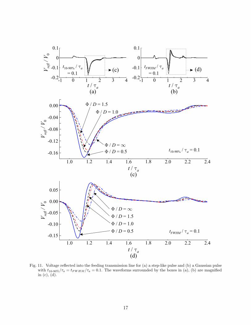
Fig. 11. Voltage reflected into the feeding transmission line for (a) a step-like pulse and (b) a Gaussian pulsewith t10-90%/τa = tFWHM/τa = 0.1. The waveforms surrounded by the boxes in (a), (b) are magnifiedin (c), (d).
17
The elliptic IRAs had larger tail waveforms than the parabolic IRA. The tail waveform
can be lowered by using an offset geometry [17]. The elliptic IRA also had larger reflected
voltages in the transmission line. The reason for this is that the negative signal from the
reflector was stronger with decreasing Φ. The reflected voltage can be lowered by refining the
shape of the TEM feed arm taper so that the positive signal from the taper is increased [18].
This increase in the positive signal will cancel the reflector signal, and therefore the reflected
voltage will be lowered. Another possibility is to use distributed impedance at the TEM
feed arm termination as shown in [19] for a parabolic reflector. In [19], the time domain
reflectometry measurement data was seen to be quite flat, and therefore the reflected voltage
in the transmission line is low.
V. Acknowledgement
This work is supported in part by the US Army CECOM RDEC Night Vision and
Electronic Sensors Directorate, Countermine Division.
18
References
1. C. E. Baum and E. G. Farr, “Impulse radiating antennas,” in Ultra-Wideband, ShortPulse Electromagnetics. H. Bertoni et al., Eds. New York: Plenum, 1993, pp. 139–147.
2. E. G. Farr, C. E. Baum, and C. J. Buchenauer, “Impulse radiating antennas, part II,”in Ultra-Wideband, Short Pulse Electromagnetics 2. L. Carin and L. B. Felsen, Eds.New York: Plenum, 1995, pp. 159–170.
3. D. V. Giri, H. Lackner, I. D. Smith, D. W. Morton, C. E. Baum, J. R. Marek, W. D.Prather, and D. W. Scholfield, “Design, fabrication, and testing of a paraboloidal reflec-tor antenna and pulser system for impulse-like waveforms,” IEEE Trans. Plasma Sci.,vol. 25, no. 2, pp. 318–326, Apr. 1997.
4. C. E. Baum, E. G. Farr, and D. V. Giri, “Review of impulse-radiating antennas,” inReviw of Radio Science 1996-1999. W. R. Stone, Ed. Oxford University Press, 1999,ch. 16, pp. 403–439.
5. E. G. Farr and L. H. Bowen, “Impulse radiating antennas for mine detection,” in De-tection and Remediation Technologies for Mines and Minelike Targets VI, Proc. SPIE,vol. 4394, Apr. 2001, pp. 680–691.
6. J. R. R. Pressley, D. Pabst, G. Sower, L. Nee, B. Green, and P. Howard, “Ground stand-off mine detection system (GSTAMIDS) engineering, manufacturing and development(EMD) block 0,” in Detection and Remediation Technologies for Mines and MinelikeTargets VI, Proc. SPIE, vol. 4394, Apr. 2001, pp. 1190–1200.
7. G. Sower, J. Eberly, and E. Christy, “GSTAMIDS ground-penetrating radar: hardwaredescription,” in Detection and Remediation Technologies for Mines and Minelike TargetsVI, Proc. SPIE, vol. 4394, Apr. 2001, pp. 651–661.
8. K. Kim and W. R. Scott, Jr., “Numerical analysis of the impulse-radiating antenna,”Sensor and Simulation Notes #474, June 3, 2003.
9. K. Hirasawa, K. Fujimoto, T. Uchikura, S. Hirafuku, and H. Naito, “Power focusingcharacteristics of ellipsoidal reflector,” IEEE Trans. Antennas Propagat., vol. AP-32,no. 10, pp. 1033–1039, Oct. 1984.
10. R. M. Sharpe, J. B. Grant, N. J. Champagne, W. A. Johnson, R. E. Jorgenson, D. R.Wilton, W. J. Brown, and J. W. Rockway, “EIGER: Electromagnetic interactions gen-eralized,” in IEEE AP-S Int’l Symp. Digest, Quebec, Canada, Jul. 1997, pp. 2366–2369.
11. Lawrence Livermore National Laboratory. (2001, March 5) EIGER - A Revolution inComputational Electromagnetics. [Online]. Available: http://cce.llnl.gov/eiger/
12. E. G. Farr and C. E. Baum, “Prepulse associated with the TEM feed of an impulse
19
radiating antenna,” Sensor and Simulation Notes #337, Mar. 1992.
13. E. G. Farr, “Optimizing the feed impedance of impulse radiating antennas, Part I:Reflector IRAs,” Sensor and Simulation Notes #354, Jan. 1993.
14. C. E. Baum, “Some topics concerning feed arms of reflector IRAs,” Sensor and Simula-tion Notes #414, Oct. 31, 1997.
15. M. Abramowitz and I. A. Stegun, Handbook of Mathematical Functions with Formulas,Graphs, and Mathematical Tables. New York: Dover, 1972.
16. J. W. Sherman, III, “Properties of focused apertures in the Fresnel region,” IRE Trans.Antennas Propagat., vol. AP-10, no. 4, pp. 399–408, Jul. 1962.
17. K. Kim and W. R. Scott, Jr., “Analysis of an offset impulse-radiating antenna,” Sensorand Simulation Notes #476, June 16, 2003.
18. K. Kim, “Numerical and experimental investigation of impulse-radiating antennas foruse in sensing applications,” Ph.D. dissertation, Georgia Institute of Technology, April2003.
19. M. Abdalla, M. Skipper, D. V. Giri, H. La Valley, T. Smith, D. McLemore, J. Burger,R. Torres, T. Tran, W. Prather, and C. E. Baum, “Evaluation of the terminatingimpedance in the conical-line feed of the 6-foot IRA,” Prototype IRA Memos #8, Apr.15, 2001.
20