arX

iv:0

709.

2791

v1 [

mat

h.O

C]

18 S

ep 2

007

Report no. 07/18

Kalman Filtering with Equality and Inequality StateConstraints

Nachi Gupta Raphael HauserOxford University Computing Laboratory, Numerical Analysis Group,

Wolfson Building, Parks Road, Oxford OX1 3QD, U.K.

Both constrained and unconstrained optimization problemsregularly appearin recursive tracking problems engineers currently address – however, constraintsare rarely exploited for these applications. We define the Kalman Filter anddiscuss two different approaches to incorporating constraints. Each of these ap-proaches are first applied to equality constraints and then extended to inequalityconstraints. We discuss methods for dealing with nonlinearconstraints and forconstraining the state prediction. Finally, some experiments are provided to indi-cate the usefulness of such methods.

Key words and phrases:Constrained optimization, Kalman filtering, Nonlinear filters,Optimization methods, Quadratic programming, State estimation

The first author would like to thank the Clarendon Bursary forfinancial support.

Oxford University Computing LaboratoryNumerical Analysis GroupWolfson BuildingParks RoadOxford, England OX1 3QDE-mail: nachi@comlab.oxford.ac.uk February, 2008

2

1 Introduction

Kalman Filtering [8] is a method to make real-time predictions for systems with some knowndynamics. Traditionally, problems requiring Kalman Filtering have been complex and non-linear. Many advances have been made in the direction of dealing with nonlinearities (e.g.,Extended Kalman Filter [1], Unscented Kalman Filter [7]). These problems also tend to haveinherent state spaceequalityconstraints (e.g., a fixed speed for a robotic arm) and state spaceinequalityconstraints (e.g., maximum attainable speed of a motor). Inthe past, less interesthas been generated towards constrained Kalman Filtering, partly because constraints can bedifficult to model. As a result, constraints are often neglected in standard Kalman Filteringapplications.

The extension to Kalman Filtering with known equality constraints on the state space isdiscussed in [5, 11, 13, 14, 16]. In this paper, we discuss twodistinct methods to incorporateconstraints into a Kalman Filter. Initially, we discuss these in the framework of equality con-straints. The first method, projecting the updated state estimate onto the constrained region,appears with some discussion in [5, 11]. We propose another method, which is to restrict theoptimal Kalman Gain so the updated state estimate will not violate the constraint. With somealgebraic manipulation, the second method is shown to be a special case of the first method.

We extend both of these concepts to Kalman Filtering with inequality constraints in thestate space. This generalization for the first approach was discussed in [12].1 Constraining theoptimal Kalman Gain was briefly discussed in [10]. Further, we will also make the extensionto incorporating state space constraints in Kalman Filter predictions.

Analogous to the way a Kalman Filter can be extended to solve problems containing non-linearities in the dynamics using an Extended Kalman Filterby linearizing locally (or by usingan Unscented Kalman Filter), linear inequality constrained filtering can similarly be extendedto problems with nonlinear constraints by linearizing locally (or by way of another schemelike an Unscented Kalman Filter). The accuracy achieved by methods dealing with nonlinearconstraints will naturally depend on the structure and curvature of the nonlinear function it-self. In the two experiments we provide, we look at incorporating inequality constraints to atracking problem with nonlinear dynamics.

2 Kalman Filter

A discrete-time Kalman Filter [8] attempts to find the best running estimate for a recursivesystem governed by the following model2:

xk = Fk,k−1xk−1 +uk,k−1, uk,k−1 ∼ N(

0,Qk,k−1)

(2.1)

zk = Hkxk +vk, vk ∼ N (0,Rk) (2.2)

1The similar extension for the method of [16] was made in [6].2The subscriptk on a variable stands for thek-th time step, the mathematical notationN (µ ,Σ) denotes a

normally distributed random vector with meanµ and covarianceΣ, and all vectors in this paper are columnvectors (unless we are explicitly taking the transpose of the vector).

3

Herexk is ann-vector that represents the true state of the underlying system andFk,k−1is ann×n matrix that describes the transition dynamics of the systemfrom xk−1 to xk. Themeasurement made by the observer is anm-vectorzk, andHk is anm×n matrix that trans-forms a vector from the state space into the appropriate vector in the measurement space. Thenoise termsuk,k−1 (ann-vector) andvk (anm-vector) encompass known and unknown errorsin Fk,k−1 andHk and are normally distributed with mean 0 and covariances given byn× nmatrix Qk,k−1 andm×m matrix Rk, respectively. At each iteration, the Kalman Filter makesa state prediction forxk, denoted ˆxk|k−1. We use the notationk|k−1 since we will only usemeasurements provided until time-stepk−1 in order to make the prediction at time-stepk.The state prediction error ˜xk|k−1 is defined as the difference between the true state and thestate prediction, as below.

xk|k−1 = xk− xk|k−1 (2.3)

The covariance structure for the expected error on the stateprediction is defined as theexpectation of the outer product of the state prediction error. We call this covariance structurethe error covariance prediction and denote itPk|k−1.3

Pk|k−1 = E

[

(

xk|k−1)(

xk|k−1)′

]

(2.4)

The filter will also provide an updated state estimate forxk, given all the measurementsprovided up to and including time stepk. We denote these estimates by ˆxk|k. We similarlydefine the state estimate error ˜xk|k as below.

xk|k = xk− xk|k (2.5)

The expectation of the outer product of the state estimate error represents the covariancestructure of the expected errors on the state estimate, which we call the updated error covari-ance and denotePk|k.

Pk|k = E

[

(

xk|k)(

xk|k)′

]

(2.6)

At time-stepk, we can make a prediction for the underlying state of the system by allowingthe state to transition forward using our model for the dynamics and noting thatE

[

uk,k−1]

= 0.This serves as our state prediction.

xk|k−1 = Fk,k−1xk−1|k−1 (2.7)

If we expand the expectation in Equation (2.4), we have the following equation for theerror covariance prediction.

Pk|k−1 = Fk,k−1Pk−1|k−1F ′k,k−1 +Qk,k−1 (2.8)

We can transform our state prediction into the measurement space, which is a predictionfor the measurement we now expect to observe.

3We use the prime notation on a vector or a matrix to denote its transpose throughout this paper.

4

zk|k−1 = Hkxk|k−1 (2.9)

The difference between the observed measurement and our predicted measurement is themeasurement residual, which we are hoping to minimize in this algorithm.

νk = zk− zk|k−1 (2.10)

We can also calculate the associated covariance for the measurement residual, which is theexpectation of the outer product of the measurement residual with itself, E

[

νkν ′k

]

. We call thisthe measurement residual covariance.

Sk = HkPk|k−1H ′k +Rk (2.11)

We can now define our updated state estimate as our predictionplus some perturbation,which is given by a weighting factor times the measurement residual. The weighting factor,called the Kalman Gain, will be discussed below.

xk|k = xk|k−1 +Kkνk (2.12)

Naturally, we can also calculate the updated error covariance by expanding the outer prod-uct in Equation (2.6).4

Pk|k = (I−KkHk)Pk|k−1(I−KkHk)′ +KkRkK

′k (2.13)

Now we would like to find the Kalman GainKk, which minimizes the mean square state

estimate error,E[

∣

∣xk|k

∣

∣

2]

. This is the same as minimizing the trace of the updated error

covariance matrix above.5 After some calculus, we find the optimal gain that achieves this,written below.6

Kk = Pk|k−1H ′kS

−1k (2.14)

The covariance matrices in the Kalman Filter provide us witha measure for uncertaintyin our predictions and updated state estimate. This is a veryimportant feature for the variousapplications of filtering since we then know how much to trustour predictions and estimates.Also, since the method is recursive, we need to provide an initial covariance that is largeenough to contain the initial state to ensure comprehensible performance. For a more detaileddiscussion of Kalman Filtering, we refer the reader to the following book [1].

4The I in Equation (2.13) represents then×n identity matrix. Throughout this paper, we use I to denote thesame matrix, except in Appendix A, where I is the appropriately sized identity matrix.

5Note thatv′v = trace[vv′] for some vectorv.6We could also minimize the mean square state estimate error in theN norm, whereN is a positive definite

and symmetric weighting matrix. In theN norm, the optimal gain would beKNk = N

12 Kk.

5

3 Equality Constrained Kalman Filtering

A number of approaches have been proposed for solving the equality constrained KalmanFiltering problem [5, 11, 13, 14, 16]. In this paper, we show two different methods. The firstmethod will restrict the state at each iteration to lie in theequality constrained space. Thesecond method will start with a constrained prediction, andrestrict the Kalman Gain so thatthe estimate will lie in the constrained space. Our equalityconstraints in this paper will bedefined as below, whereA is aq×n matrix,b aq-vector, andxk, the state, is an-vector.7

Axk = b (3.1)

So we would like our updated state estimate to satisfy the constraint at each iteration, asbelow.

Axk|k = b (3.2)

Similarly, we may also like the state prediction to be constrained, which would allow abetter forecast for the system.

Axk|k−1 = b (3.3)

In the following subsections, we will discuss methods for constraining the updated stateestimate. In Section 4, we will extend these concepts and formulations to the inequality con-strained case, and in Section 6, we will address the problem of constraining the prediction, aswell.

3.1 Projecting the state to lie in the constrained space

We can solve the following minimization problem for a given time-stepk, where ˆxPk|k is the

constrained estimate,Wk is any positive definite symmetric weighting matrix, and ˆxk|k is theunconstrained Kalman Filter updated estimate.

xPk|k = argmin

x∈Rn

{

(

x− xk|k)′

Wk(

x− xk|k)

: Ax= b}

(3.4)

The best constrained estimate is then given by

xPk|k = xk|k−W−1

k A′(

AW−1k A′

)−1(

Axk|k−b)

(3.5)

To find the updated error covariance matrix of the equality constrained filter, we first definethe matrixϒ below.8

ϒ = W−1k A′

(

AW−1k A′

)−1(3.6)

Equation (3.5) can then be re-written as following.

7A andb can be different for differentk. We don’t subscript eachA andb to avoid confusion.8Note thatϒA is a projection matrix, as is(I−ϒA), by definition. IfA is poorly conditioned, we can use a QR

factorization to avoid squaring the condition number.

6

xPk|k = xk|k−ϒ

(

Axk|k−b)

(3.7)

We can find a reduced form forxk− xPk|k as below.

xk− xPk|k = xk− xk|k +ϒ

(

Axk|k−b− (Axk−b))

(3.8a)

= xk− xk|k +ϒ(

Axk|k−Axk)

(3.8b)

= −(I−ϒA)(

xk|k−xk)

(3.8c)

Using the definition of the error covariance matrix, we arrive at the following expression.

PPk|k = E

[

(

xk− xPk|k

)(

xk− xPk|k

)′]

(3.9a)

= E

[

(I−ϒA)(

xk|k−xk)(

xk|k−xk)′

(I−ϒA)′]

(3.9b)

= (I−ϒA)Pk|k (I−ϒA)′ (3.9c)

= Pk|k−ϒAPk|k−Pk|kA′ϒ′+ϒAPk|kA

′ϒ′ (3.9d)

= Pk|k−ϒAPk|k (3.9e)

= (I−ϒA)Pk|k (3.9f)

It can be shown that choosingWk = P−1k|k results in the smallest updated error covariance.

This also provides a measure of the information in the state at k.9

3.2 Restricting the optimal Kalman Gain so the updated state estimatelies in the constrained space

Alternatively, we can expand the updated state estimate term in Equation (3.2) using Equation(2.12).

A(

xk|k−1 +Kkνk)

= b (3.10)

Then, we can choose a Kalman GainKRk , that forces the updated state estimate to be in

the constrained space. In the unconstrained case, we chose the optimal Kalman GainKk, bysolving the minimization problem below which yields Equation (2.14).

Kk = argminK∈Rn×m

trace[

(I−KHk)Pk|k−1(I−KHk)′+KRkK

′]

(3.11)

9If M andN are covariance matrices, we sayN is smaller thanM if M−N is positive semidefinite. Anotherformulation for incorporating equality constraints into aKalman Filter is by observing the constraints as pseudo-measurements [14, 16]. WhenWk is chosen to beP−1

k|k , both of these methods are mathematically equivalent [5].Also, a more numerically stable form of Equation (3.9) with discussion is provided in [5].

7

Now we seek the optimalKRk that satisfies the constrained optimization problem written

below for a given time-stepk.

KRk = argmin

K∈Rn×mtrace

[

(I−KHk)Pk|k−1(I−KHk)′+KRkK

′]

s.t.A(

xk|k−1 +Kνk)

= b(3.12)

We will solve this problem using the method of Lagrange Multipliers. First, we take thesteps below, using the vec notation (column stacking matrices so they appear as long vectors,see Appendix A) to convert all appearances ofK in Equation (4.8) into long vectors. Let usbegin by expanding the following term.10

trace[

(I−KHk)Pk|k−1(I−KHk)′+KRkK

′]

= trace[

Pk|k−1−KHkPk|k−1−Pk|k−1H ′kK

′+KHkPk|k−1H ′kK

′+KRkK′]

(2.11)= trace

[

Pk|k−1−KHkPk|k−1−Pk|k−1H ′kK

′+KSkK′]

= trace[

Pk|k−1]

− trace[

KHkPk|k−1]

− trace[

Pk|k−1H ′kK

′]

+ trace[

KSkK′]

(3.13a)

We now expand the last three terms in Equation (3.13a) one at atime.11

trace[

KHkPk|k−1] (A.9)

= vec[

(

HkPk|k−1)′

]′vec[K]

= vec[

Pk|k−1H ′k

]′vec[K]

(3.14)

trace[

Pk|k−1H ′kK

′] (A.9)

= vec[K]′ vec[

Pk|k−1H ′k

]

(3.15)

trace[

KSkK′] (A.9)

= vec[K]′ vec[KSk]

(A.7)= vec[K]′ (S⊗ I)vec[K]

(3.16)

Remembering that trace[

Pk|k−1]

is constant, our objective function can be written as be-low.

vec[K]′ (I⊗Sk)vec[

K′]

−vec[

Pk|k−1H ′k

]′vec[K]

−vec[K]′ vec[

Pk|k−1H ′k

] (3.17)

Using Equation (A.8) on the equality constraints, our minimization problem is the follow-ing.

10Throughout this paper, a number in parentheses above an equals sign means we made use of this equationnumber.

11We use the symmetry ofPk|k−1 in Equation (3.14) and the symmetry ofSk in Equation (3.16).

8

KRk = argmin

K∈Rn×mvec[K]′ (Sk⊗ I)vec[K]

−vec[

Pk|k−1H ′k

]′vec[K]

−vec[K]′vec[

Pk|k−1H ′k

]

s.t.(

ν ′k⊗A

)

vec[K] = b−Axk|k−1

(3.18)

Further, we simplify this problem so the minimization problem has only one quadraticterm. We complete the square as follows. We want to find the unknown variableµ which willcancel the linear term. Let the quadratic term appear as follows. Note that the non-“vec[K]"term is dropped as is is irrelevant for the minimization problem.

(vec[K]+ µ)′ (Sk⊗ I)(vec[K]+ µ) (3.19)

The linear term in the expansion above is the following.

vec[K]′ (Sk⊗ I)µ + µ ′ (Sk⊗ I)vec[K] (3.20)

So we require that the two equations below hold.

(Sk⊗ I)µ = −vec[

Pk|k−1H ′k

]

µ ′ (Sk⊗ I) = −vec[

Pk|k−1H ′k

]′ (3.21)

This leads to the following value forµ.

µ (A.3)= −

(

S−1k ⊗ I

)

vec[

Pk|k−1H ′k

]

(A.8)= −vec

[

Pk|k−1H ′kS

−1k

]

(2.14)= −vec[Kk]

(3.22)

Using Equation (A.6), our quadratic term in the minimization problem becomes the fol-lowing.

(vec[K −Kk])′ (Sk⊗ I)(vec[K −Kk]) (3.23)

Let l = vec[K −Kk]. Then our minimization problem becomes the following.

KRk = argmin

l∈Rmnl ′ (Sk⊗ I) l

s.t.(

ν ′k⊗A

)

(l +vec[Kk]) = b−Axk|k−1

(3.24)

We can then re-write the constraint taking the vec[Kk] term to the other side as below.(

ν ′k⊗A

)

l = b−Axk|k−1−(

ν ′k⊗A

)

vec[Kk]

(A.8)= b−Axk|k−1−vec[AKkνk]

= b−Axk|k−1−AKkνk

(2.12)= b−Axk|k

(3.25)

9

This results in the following simplified form.

KRk = argmin

l∈Rmnl ′ (Sk⊗ I) l

s.t.(

ν ′k⊗A

)

l = b−Axk|k

(3.26)

We form the LagrangianL , where we introduceq Lagrange Multipliers in vectorλ =(

λ1,λ2, . . . ,λq)′

L =l ′ (Sk⊗ I) l −λ ′[(

ν ′k⊗A

)

l −b+Axk|k]

(3.27)

We take the partial derivative with respect tol .12

∂L

∂ l= 2l ′ (Sk⊗ I)−λ ′

(

ν ′k⊗A

)

(3.28)

Similarly we can take the partial derivative with respect tothe vectorλ .

∂L

∂λ=

(

ν ′k⊗A

)

l −b+Axk|k (3.29)

When both of these derivatives are set equal to the appropriate size zero vector, we havethe solution to the system. Taking the transpose of Equation(3.28), we can write this systemasMn = p with the following block definitions forM,n, andp.

M =

[

2Sk⊗ I νk⊗A′

ν ′k⊗A 0[q×q]

]

(3.30)

n =

[

lλ

]

(3.31)

p =

[

0[mn×1]

b−Axk|k

]

(3.32)

We solve this system for vectorn in Appendix C. The solution forl is pasted below.([

S−1k νk

(

ν ′kS

−1k νk

)−1]

⊗[

A′(

AA′)−1

])

(

b−Axk|k)

(3.33)

Bearing in mind thatb−Axk|k = vec[

b−Axk|k]

, we can use Equation (A.8) to re-writelas below.13

vec[

A′(

AA′)−1(

b−Axk|k)(

ν ′kS

−1k νk

)−1 ν ′kS

−1k

]

(3.34)

The resulting matrix inside the vec operation is then ann by m matrix. Remembering thedefinition for l , we notice thatK −Kk results in ann by m matrix also. Since both of thecomponents inside the vec operation result in matrices of the same size, we can safely remove

12We used the symmetry of(Sk⊗ I) here.13Here we used the symmetry ofS−1

k and(

ν ′kS

−1k νk

)−1(the latter of which is actually just a scalar).

10

the vec operation from both sides. This results in the following optimal constrained KalmanGainKR

k .

Kk−A′(

AA′)−1(

Axk|k−b)(

ν ′kS

−1k νk

)−1 ν ′kS

−1k (3.35)

If we now substitute this Kalman Gain into Equation (2.12) tofind the constrained updatedstate estimate, we end up with the following.

xRk|k = xk|k−A′

(

AA′)−1(

Axk|k−b)

(3.36)

This is of course equivalent to the result of Equation (3.5) with the weighting matrixWk

chosen as the identity matrix. The error covariance for thisestimate is given by Equation(3.9).14

4 Adding Inequality Constraints

In the more general case of this problem, we may encounter equality and inequality constraints,as given below.15

Axk = b

Cxk ≤ d(4.1)

So we would like our updated state estimate to satisfy the constraint at each iteration, asbelow.

Axk|k = b

Cxk|k ≤ d(4.2)

Similarly, we may also like the state prediction to be constrained, which would allow abetter forecast for the system.

Axk|k−1 = b

Cxk|k−1 ≤ d(4.3)

We will present two analogous methods to those presented forthe equality constrainedcase. In the first method, we will run the unconstrained filter, and at each iteration constrainthe updated state estimate to lie in the constrained space. In the second method, we willfind a Kalman GainKR

k such that the the updated state estimate will be forced to liein theconstrained space. In both methods, we will no longer be ableto find an analytic solution asbefore. Instead, we use numerical methods.

14We can use the unconstrained or constrained Kalman Gain to find this error covariance matrix. Since theconstrained Kalman Gain is suboptimal for the unconstrained problem, before projecting onto the constrainedspace, the constrained covariance will be different from the unconstrained covariance. However, the differencelies exactly in the space orthogonal to which the covarianceis projected onto by Equation (3.9). The proof isomitted for brevity.

15C andd can be different for differentk. We don’t subscript eachC andd to simplify notation.

11

4.1 By Projecting the Unconstrained Estimate

Given the best unconstrained estimate, we could solve the following minimization problemfor a given time-stepk, where ˇxP

k|k is the inequality constrained estimate andWk is any positivedefinite symmetric weighting matrix.

xPk|k = argmin

x

(

x− xk|k)′

Wk(

x− xk|k)

s.t.Ax= b

Cx≤ d

(4.4)

For solving this inequality constrained optimization problem, we can use a variety of stan-dard methods, or even an out-of-the-box solver, likefmincon in Matlab. Here we use an ac-tive set method [4]. This is a common method for dealing with inequality constraints, wherewe treat a subset of the constraints (called the active set) as additional equality constraints.We ignore any inactive constraints when solving our optimization problem. After solving theproblem, we check if our solution lies in the space given by the inequality constraints. If itdoesn’t, we start from the solution in our previous iteration and move in the direction of thenew solution until we hit a set of constraints. For each iteration, the active set is made up ofthose inequality constraints with non-zero Lagrange Multipliers.

We first find the best estimate (using Equation (3.5) for the equality constrained problemwith the equality constraints given in Equation (4.1) plus the active set of inequality constraints.Let us call the solution to this ˇxP∗

k|k, j since we have not yet checked if the solution lies in the

inequality constrained space.16 In order to check this, we find the vector that we moved alongto reach ˇxP∗

k|k, j . This is given by the following.

s= xP∗k|k, j − xP

k|k, j−1 (4.5)

We now iterate through each of our inequality constraints, to check if they are satisfied. Ifthey are all satisfied, we chooseτmax = 1. If they are not, we choose the largest value ofτmax

such that ˆxk|k, j−1 + τmaxs lies in the inequality constrained space. We choose our estimate tobe

xPk|k, j = xP

k|k, j−1 + τmaxs (4.6)

If we find the solution has converged within a pre-specified error, or we have reached apre-specified maximum number of iterations, we choose this as the updated state estimate toour inequality constrained problem, denoted ˇxP

k|k. If we would like to take a further iteration

on j, we check the Lagrange Multipliers at this new solution to determine the new active set.17

We then repeat by finding the best estimate for the equality constrained problem includingthe new active set as additional equality constraints. Since this is a Quadratic Programmingproblem, each step ofj guarantees the same estimate or a better estimate.

16For the inequality constrained filter, we allow multiple iterations within each step. Thej subscript indexesthese further iterations.

17The previous active set is not relevant.

12

When calculating the error covariance matrix for this estimate, we can also add on thesafety term below.

(

xPk|k, j − xP

k|k, j−1

)(

xPk|k, j − xP

k|k, j−1

)′(4.7)

This is a measure of our convergence error and should typically be small relative to theunconstrained error covariance. We can then use Equation (3.9) to project the covariancematrix onto the constrained subspace, but we only use the defined equality constraints. We donot incorporate any constraints in the active set when computing Equation (3.9) since thesestill represent inequality constraints on the state. Ideally we would project the error covariancematrix into the inequality constrained subspace, but this projection is not trivial.

4.2 By Restricting the Optimal Kalman Gain

We could solve this problem by restricting the optimal Kalman gain also, as we did for equalityconstraints previously. We seek the optimalKk that satisfies the constrained optimizationproblem written below for a given time-stepk.

KRk = argmin

K∈Rn×mtrace

[

(I−KHk)Pk|k−1(I−KHk)′ +KRkK

′]

s.t. A(

xk|k−1 +Kkνk)

= b

C(

xk|k−1 +Kkνk)

≤ d

(4.8)

Again, we can solve this problem using any inequality constrained optimization method(e.g.,fmincon in Matlab or the active set method used previously). Here we solved theoptimization problem using SDPT3, a Matlab package for solving semidefinite programmingproblems [15]. When calculating the covariance matrix for the inequality constrained estimate,we use the restricted Kalman Gain. Again, we can add on the safety term for the convergenceerror, by taking the outer product of the difference betweenthe updated state estimates cal-culated by the restricted Kalman Gain for the last two iterations of SDPT3. This covariancematrix is then projected onto the subspace as in Equation (3.9) using the equality constraintsonly.

5 Dealing with Nonlinearities

Thus far, in the Kalman Filter we have dealt with linear models and constraints. A numberof methods have been proposed to handle nonlinear models (e.g., Extended Kalman Filter [1],Unscented Kalman Filter [7]). In this paper, we will focus onthe most widely used of these, theExtended Kalman Filter. Let’s re-write the discrete unconstrained Kalman Filtering problemfrom Equations (2.1) and (2.2) below, incorporating nonlinear models.

xk = fk,k−1(xk−1)+uk,k−1, uk,k−1 ∼ N(

0,Qk,k−1)

(5.1)

zk = hk (xk)+vk, vk ∼ N (0,Rk) (5.2)

13

In the above equations, we see that the transition matrixFk,k−1 has been replaced by thenonlinear vector-valued functionfk,k−1(·), and similarly, the matrixHk, which transforms avector from the state space into the measurement space, has been replaced by the nonlinearvector-valued functionhk (·). The method proposed by the Extended Kalman Filter is to lin-earize the nonlinearities about the current state prediction (or estimate). That is, we chooseFk,k−1 as the Jacobian offk,k−1 evaluated at ˆxk−1|k−1, andHk as the Jacobian ofhk evaluated atxk|k−1 and proceed as in the linear Kalman Filter of Section 2.18 Numerical accuracy of thesemethods tends to depend heavily on the nonlinear functions.If we have linear constraintsbut a nonlinearfk,k−1(·) andhk (·), we can adapt the Extended Kalman Filter to fit into theframework of the methods described thus far.

5.1 Nonlinear Equality and Inequality Constraints

Since equality and inequality constraints we model are often times nonlinear, it is important tomake the extension to nonlinear equality and inequality constrained Kalman Filtering for themethods discussed thus far. Without loss of generality, ourdiscussion here will pertain only tononlinear inequality constraints. We can follow the same steps for equality constraints.19 Wereplace the linear inequality constraint on the state spaceby the following nonlinear inequal-ity constraintc(xk) = d, wherec(·) is a vector-valued function. We can then linearize ourconstraint,c(xk) = d, about the current state prediction ˆxk|k−1, which gives us the following.20

c(

xk|k−1)

+C(

xk− xk|k−1)

/ d (5.3)

HereC is defined as the Jacobian ofc evaluated at ˆxk|k−1. This indicates then, that thenonlinear constraint we would like to model can be approximated by the following linearconstraint

Cxk / d+Cxk|k−1−c(

xk|k−1)

(5.4)

This constraint can be written asCxk ≤ d, which is an approximation to the nonlinearinequality constraint. It is now in a form that can be used by the methods described thus far.

The nonlinearities in both the constraints and the models,fk,k−1 (·) andhk (·), could havebeen linearized using a number of different methods (e.g., aderivative-free method, a higherorder Taylor approximation). Also an iterative method could be used as in the Iterated Ex-tended Kalman Filter [1].

18We can also do a midpoint approximation to findFk,k−1 by evaluating the Jacobian at(

xk−1|k−1 + xk|k−1)

/2.This should be a much closer approximation to the nonlinear function. We use this approximation for the Ex-tended Kalman Filter experiments later.

19We replace the ‘≤’ sign with an ‘=’ sign and the ‘/’ with an ‘≈’ sign.20This method is how the Extended Kalman Filter linearizes nonlinear functions forfk,k−1 (·) andhk (·). Here

xk|k−1 can be the state prediction of any of the constrained filters presented thus far and does not necessarily relateto the unconstrained state prediction.

14

6 Constraining the State Prediction

We haven’t yet discussed whether the state prediction (Equation (2.7)) also should be con-strained. Forcing the constraints should provide a better prediction (which is used for fore-casting in the Kalman Filter). Ideally, the transition matrix Fk,k−1 will take an updated stateestimate satisfying the constraints at timek−1 and make a prediction that will satisfy the con-straints at timek. Of course this may not be the case. In fact, the constraints may depend on theupdated state estimate, which would be the case for nonlinear constraints. On the downside,constraining the state prediction increases computational cost per iteration.

We propose three methods for dealing with the problem of constraining the state predic-tion. The first method is to project the matrixFk,k−1 onto the constrained space. This is onlypossible for the equality constraints, as there is no trivial way to projectFk,k−1 to an inequal-ity constrained space. We can use the same projector as in Equation (3.9f) so we have thefollowing.21

FPk,k−1 = (I−ϒA)Fk,k−1 (6.1)

Under the assumption that we have constrained our updated state estimate, this new transi-tion matrix will make a prediction that will keep the estimate in the equality constrained space.Alternatively, if we weaken this assumption, i.e., we are not constraining the updated stateestimate, we could solve the minimization problem below (analogous to Equation (3.4)). Wecan also incorporate inequality constraints now.

xPk|k−1 = argmin

x

(

x− xk|k−1)′

Wk(

x− xk|k−1)

s.t.Ax= b

Cx≤ d

(6.2)

We can constrain the covariance matrix here also, in a similar fashion to the method de-scribed in Section 4.1. The third method is to add to the constrained problem the additionalconstraints below, which ensure that the chosen estimate will produce a prediction at the nextiteration that is also constrained.

Ak+1Fk+1,kxk = bk+1

Ck+1Fk+1,kxk ≤ dk+1(6.3)

If Ak+1,bk+1,Ck+1 or dk+1 depend on the estimate (e.g., if we are linearizing nonlinearfunctionsa(·) or b(·), we can use an iterative method, which would resolveAk+1 andbk+1using the current best updated state estimate (or prediction), re-calculate the best estimateusingAk+1 andbk+1, and so forth until we are satisfied with the convergence. This methodwould be preferred since it looks ahead one time-step to choose a better estimate for the currentiteration.22 However, it can be far more expensive computationally.

21In these three methods, the symmetric weighting matrixWk can be different. The resultingϒ can conse-quently also be different.

22Further, we can add constraints for some arbitraryn time-steps ahead.

15

7 Experiments

We provide two related experiments here. We have a car driving along a straight road withthickness 2 meters. The driver of the car traces a noisy sine curve (with the noise lying only inthe frequency domain). The car is tagged with a device that transmits the location within someknown error. We would like to track the position of the car. Inthe first experiment, we filterover the noisy data with the knowledge that the underlying function is a noisy sine curve. Theinequality constrained methods will constrain the estimates to only take values in the interval[−1,1]. In the second experiment, we do not use the knowledge that the underlying curve is asine curve. Instead we attempt to recover the true data usingan autoregressive model of order6 [3]. We do, however, assume our unknown function only takesvalues in the interval[−1,1],and we can again enforce these constraints when using the inequality constrained filter.

The driver’s path is generated using the nonlinear stochastic process given by Equation(5.1). We start with the following initial point.

x0 =

[

0 m0 m

]

(7.1)

Our vector-valued transition function will depend on a discretization parameterT and canbe expressed as below. Here, we chooseT to beπ/10, and we run the experiment from aninitial time of 0 to a final time of 10π .

fk,k−1 =

[

(xk−1)1 +Tsin((xk−1)1+T)

]

(7.2)

And for the process noise we choose the following.

Qk,k−1 =

[

0.1 m2 00 0 m2

]

(7.3)

The driver’s path is drawn out by the second element of the vector xk – the first elementacts as an underlying state to generate the second element, which also allows a natural methodto add noise in the frequency domain of the sine curve while keeping the process recursivelygenerated.

7.1 First Experiment

To create the measurements, we use the model from Equation (2.2), whereHk is the squareidentity matrix of dimension 2. We chooseRk as below to noise the data. This considerablymasks the true underlying data as can be seen in Fig. 1.23

Rk =

[

10 m2 00 10 m2

]

(7.4)

23The figure only shows the noisy sine curve, which is the secondelement of the measurement vector. Thefirst element, which is a noisy straight line, isn’t plotted.

16

0 5 10 15 20 25 30-8

-6

-4

-2

0

2

4

6

8

(met

ers)

Noisy Measurements

Time (seconds)

Figure 1: We take our sine curve, which is already noisy in the frequency domain (due to process noise),and add measurement noise. The underlying sine curve is significantly masked.

For the initial point of our filters, we choose the following point, which is different fromthe true initial point given in Equation (7.1).

x0|0 =

[

0 m1 m

]

(7.5)

Our initial covariance is given as below.24.

P0|0 =

[

1 m2 0.10.1 1 m2

]

(7.6)

24Nonzero off-diagonal elements in the initial covariance matrix often help the filter converge more quickly

17

In the filtering, we use the information that the underlying function is a sine curve, and ourtransition functionfk,k−1 changes to reflect a recursion in the second element ofxk – now wewill add on discretized pieces of a sine curve to our previousestimate. The function is givenexplicitly below.

fk,k−1 =

[

(xk−1)1 +T(xk−1)1+sin((xk−1)1+T)−sin((xk−1)1)

]

(7.7)

For the Extended Kalman Filter formulation, we will also require the Jacobian of thismatrix denotedFk,k−1, which is given below.

Fk,k−1 =

[

1 0cos((xk−1)1 +T)−cos((xk−1)1) 1

]

(7.8)

The process noiseQk,k−1, given below, is chosen similar to the noise used in generatingthe simulation, but is slightly larger to encompass both thenoise in our above model and toprevent divergence due to numerical roundoff errors. The measurement noiseRk is chosen thesame as in Equation (7.4).

Qk,k−1 =

[

0.1 m2 00 0.1 m2

]

(7.9)

The inequality constraints we enforce can be expressed using the notation throughout thechapter, withC andd as given below.

C =

[

0 10 −1

]

(7.10)

d =

[

11

]

(7.11)

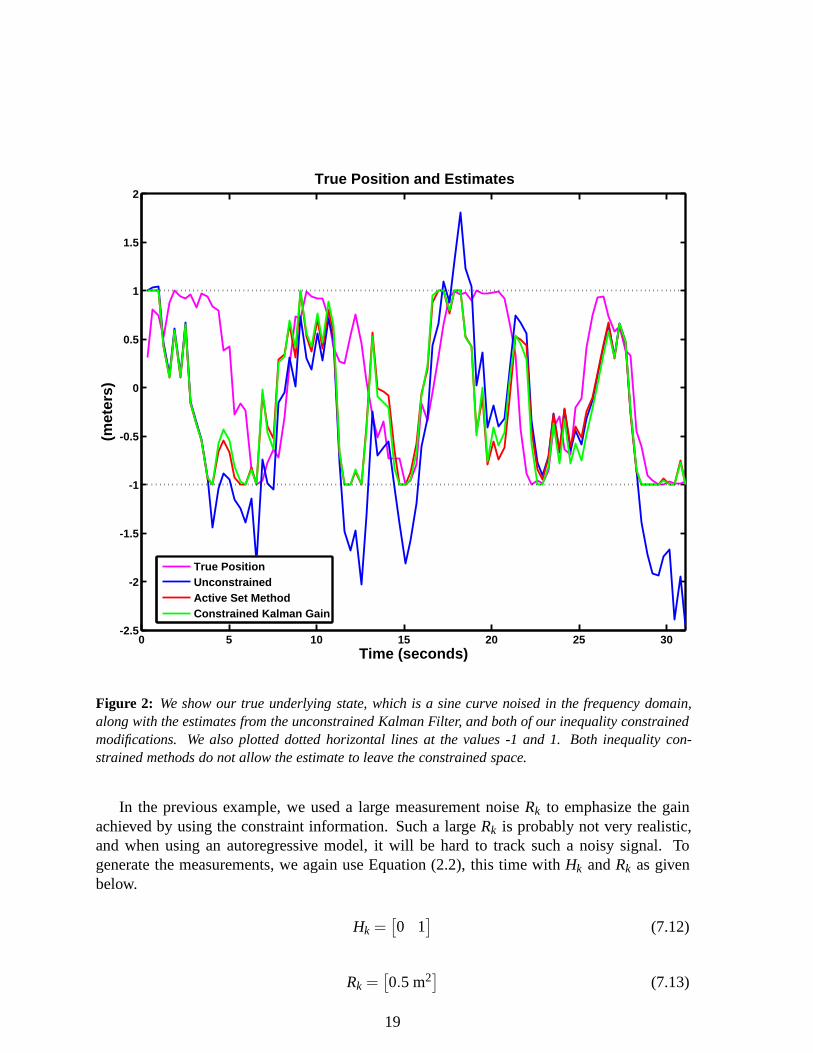
These constraints force the second element of the estimatexk|k (the sine portion) to lie inthe interval[−1,1]. We do not have any equality constraints in this experiment.We run theunconstrained Kalman Filter and both of the constrained methods discussed previously. A plotof the true position and estimates is given in Fig. 2. Notice that both constrained methods forcethe estimate to lie within the constrained space, while the unconstrained method can violatethe constraints.

7.2 Second Experiment

In the previous experiment, we used the knowledge that the underlying function was a noisysine curve. If this is not known, we face a significantly harder estimation problem. Let usassume nothing about the underlying function except that itmust take values in the interval[−1,1]. A good model for estimating such an unknown function could be an autoregressivemodel. We can compare the unconstrained filter to the two constrained methods again usingthese assumption and an autoregressive model of order 6, or AR(6) as it is more commonlyreferred to.

18

0 5 10 15 20 25 30-2.5

-2

-1.5

-1

-0.5

0

0.5

1

1.5

2

(met

ers)

True Position and Estimates

Time (seconds)

True PositionUnconstrainedActive Set MethodConstrained Kalman Gain

Figure 2: We show our true underlying state, which is a sine curve noised in the frequency domain,along with the estimates from the unconstrained Kalman Filter, and both of our inequality constrainedmodifications. We also plotted dotted horizontal lines at the values -1 and 1. Both inequality con-strained methods do not allow the estimate to leave the constrained space.

In the previous example, we used a large measurement noiseRk to emphasize the gainachieved by using the constraint information. Such a largeRk is probably not very realistic,and when using an autoregressive model, it will be hard to track such a noisy signal. Togenerate the measurements, we again use Equation (2.2), this time withHk andRk as givenbelow.

Hk =[

0 1]

(7.12)

Rk =[

0.5 m2]

(7.13)

19

Our state will now be defined using the following 13-vector, in which the first element isthe current estimate, the next five elements are lags, the sixelements afterwards are coefficientson the current estimate and the lags, and the last element is aconstant term.

xk|k =[

yk yk−1 · · · yk−5 α1 α2 · · · α7]′

(7.14)

Our matrixHk in the filter is a row vector with the first element 1, and all therest as 0, soyk|k−1 is actually our prediction ˆzk|k−1 in the filter, describing where we believe the expectedvalue of the next point in the time-series to lie. For the initial state, we choose a vector of allzeros, except the first and seventh element, which we choose as 1. This choice for the initialconditions leads to the first prediction on the time series being 1, which is incorrect as the trueunderlying state has expectation 0. For the initial covariance, we choose I[13×13] and add 0.1to all the off-diagonal elements.25 The transition functionfk,k−1 for the AR(6) model is givenbelow.

min(1,max(−1,α1yk−1 + · · ·+α6yk−6 +α7))min(1,max(−1,yk−1))min(1,max(−1,yk−2))min(1,max(−1,yk−3))min(1,max(−1,yk−4))min(1,max(−1,yk−5))

α1

α2...

α6α7

(7.15)

Putting this into recursive notation, we have the following.

min(1,max(−1,(xk−1)7(xk−1)1 + · · ·+(xk−1)13))min(1,max(−1,(xk−1)1))min(1,max(−1,(xk−1)2))min(1,max(−1,(xk−1)3))min(1,max(−1,(xk−1)4))min(1,max(−1,(xk−1)5))

(xk−1)7(xk−1)8

...(xk−1)12(xk−1)13

(7.16)

The Jacobian offk,k−1 is given below. We ignore the min(·) and max(·) operators sincethe derivative is not continuous across them, and we can reach the bounds by numerical error.

25The bracket subscript notation is used through the remainder of this paper to indicate the size of zero matricesand identity matrices.

20

Further, when enforced, the derivative would be 0, so by ignoring them, we are allowing ourcovariance matrix to be larger than necessary as well as morenumerically stable.

(xk−1)7 · · · (xk−1)12

I[5×5] 0[5×1]

(xk−1)1 · · · (xk−1)6 1

0[5×7]

0[7×6] I[7×7]

(7.17)

For the process noise, we chooseQk,k−1 to be a diagonal matrix with the first entry as 0.1and all remaining entries as 10−6 since we know the prediction phase of the autoregressivemodel very well. The inequality constraints we enforce can be expressed using the notationthroughout the chapter, withC as given below andd as a 12-vector of ones.

C =

[

I[6×6]

− I [6×6]0[12×7]

]

(7.18)

These constraints force the current estimate and all of the lags to take values in the range[−1,1]. As an added feature of this filter, we are also estimating thelags at each iteration usingmore information although we don’t use it – this is a fixed interval smoothing. In Fig. 3, weplot the noisy measurements, true underlying state, and thefilter estimates. Notice again thatthe constrained methods keep the estimates in the constrained space. Visually, we can see theimprovement particularly near the edges of the constrainedspace.

8 Conclusions

We’ve provided two different formulations for including constraints into a Kalman Filter. Inthe equality constrained framework, these formulations have analytic formulas, one of whichis a special case of the other. In the inequality constrainedcase, we’ve shown two numericalmethods for constraining the estimate. We also discussed how to constrain the state predictionand how to handle nonlinearities. Our two examples show thatthese methods ensure theestimate lies in the constrained space, which provides a better estimate structure.

Appendix A Kron and Vec

In this appendix, we provide some definitions used earlier inthe chapter. Given matrixA ∈R

m×n andB∈ Rp×q, we can define the right Kronecker product as below.26

(A⊗B) =

a1,1B · · · a1,nB...

. . ....

am,1B · · · am,nB

(A.1)

26The indicesm,n, p, andq and all matrix definitions are independent of any used earlier. Also, the subscriptnotationa1,n denotes the element in the first row andn-th column ofA, and so forth.

21

0 5 10 15 20 25 30-3

-2

-1

0

1

2

3

(met

ers)

Measurement, True Position, and Estimates

Time (seconds)

Noisy MeasurementTrue PositionUnconstrainedActive Set MethodConstrained Kalman Gain

Figure 3: We show our true underlying state, which is a sine curve noised in the frequency domain, thenoised measurements, and the estimates from the unconstrained and both inequality constrained filters.We also plotted dotted horizontal lines at the values -1 and 1. Both inequality constrained methods donot allow the estimate to leave the constrained space.

Given appropriately sized matricesA,B,C, andD such that all operations below are well-defined, we have the following equalities.

(A⊗B)′ =(

A′⊗B′)

(A.2)

(A⊗B)−1 =(

A−1⊗B−1) (A.3)

(A⊗B)(C⊗D) = (AC⊗BD) (A.4)

22

We can also define the vectorization of an[m×n] matrixA, which is a linear transformationon a matrix that stacks the columns iteratively to form a longvector of size[mn×1], as below.

vec[A] =

a1,1...

am,1a1,2

...am,2

...a1,n

...am,n

(A.5)

Using the vec operator, we can state the trivial definition below.

vec[A+B] = vec[A]+vec[B] (A.6)

Combining the vec operator with the Kronecker product, we have the following.

vec[AB] =(

B′⊗ I)

vec[A] (A.7)

vec[ABC] =(

C′⊗A)

vec[B] (A.8)

We can express the trace of a product of matrices as below.

trace[AB] = vec[

B′]′

vec[A] (A.9)

trace[ABC] = vec[B]′ (I⊗C)vec[A] (A.10a)

= vec[A]′ (I⊗B)vec[C] (A.10b)

= vec[A]′ (C⊗ I)vec[B] (A.10c)

For more information, please see [9].

Appendix B Analytic Block Representation for the inverseof a Saddle Point Matrix

MS is a saddle point matrix if it has the block form below.27

27The subscriptSnotation is used to differentiate these matrices from any matrices defined earlier.

23

MS =

[

AS B′S

BS −CS

]

(B.1)

In the case thatAS is nonsingular and the Schur complementJS = −(

CS+BSA−1S B′

S

)

isalso nonsingular in the above equation, it is known that the inverse of this saddle point matrixcan be expressed analytically by the following equation (see e.g., [2]).

M−1S =

[

A−1S +A−1

S B′SJ−1

S BSA−1S −A−1

S B′SJ−1

S−J−1

S BSA−1S J−1

S

]

(B.2)

Appendix C Solution to the system Mn = p

Here we solve the systemMn = p from Equations (3.30), (3.31), and (3.32), re-stated below,for vectorn.

[

2Sk⊗ I νk⊗A′

ν ′k⊗A 0[q×q]

][

lλ

]

=

[

0[mn×1]

b−Axk|k

]

(C.1)

M is a saddle point matrix with the following equations to fit the block structure of Equa-tion (B.1).28

AS = 2Sk⊗ I (C.2)

BS = ν ′k⊗A (C.3)

CS = 0[q×q] (C.4)

We can calculate the termA−1S B′

S.

A−1S B′

S = [2(Sk⊗ I)]−1(

ν ′k⊗A

)′(C.5a)

(A.2)(A.3)=

12

(

S−1k ⊗ I

)(

νk⊗A′)

(C.5b)

(A.4)=

12

(

S−1k νk

)

⊗A′ (C.5c)

And as a result we have the following forJS.

JS = −12

(

ν ′k⊗A

)[(

S−1k νk

)

⊗A′]

(C.6a)

(A.4)= −

12

(

ν ′kS

−1k νk

)

⊗(

AA′)

(C.6b)

28We use Equation (A.2) withB′S to arrive at the same term forBs in Equation (C.1).

24

J−1S is then, as below.

J−1S = −2

[(

ν ′kS

−1k νk

)

⊗(

AA′)]−1

(C.7a)(A.3)= −2

(

ν ′kS

−1k νk

)−1⊗

(

AA′)−1

(C.7b)

For the upper right block ofM−1, we then have the following expression.

A−1S B′

SJ−1S =

[(

S−1k νk

)

⊗A′]

[

(

ν ′kS

−1k νk

)−1⊗

(

AA′)−1

]

(C.8a)

(A.4)=

[

S−1k νk

(

ν ′kS

−1k νk

)−1]

⊗[

A′(

AA′)−1

]

(C.8b)

Since the first block element ofp is a vector of zeros, we can solve forn to arrive at thefollowing solution forl .

([

S−1k νk

(

ν ′kS

−1k νk

)−1]

⊗[

A′(

AA′)−1

])

(

b−Axk|k)

(C.9)

The vector of Lagrange Multipliersλ is given below.

−2[

(

ν ′kS

−1k νk

)−1⊗

(

AA′)−1

]

(

b−Axk|k)

(C.10)

References

[1] Y. BAR-SHALOM , X. R. LI , AND T. K IRUBARAJAN, Estimation with Applications toTracking and Navigation, John Wiley and Sons, Inc., 2001.

[2] M. BENZI, G. H. GOLUB, AND J. LIESEN, Numerical solution of saddle point problems,Acta Numerica, 14 (2005), pp. 1–137.

[3] G. E. P. BOX AND G. M. JENKINS, Time Series Analysis. Forecasting and Control(Revised Edition), Oakland: Holden-Day, (1976).

[4] R. FLETCHER, Practical methods of optimization. Vol. 2: Constrained Optimiza-tion, John Wiley & Sons Ltd., Chichester, 1981. Constrained optimization, A Wiley-Interscience Publication.

[5] N. GUPTA, Kalman filtering in the presence of state space equality constraints, inIEEE Proceedings of the 26th Chinese Control Conference, July 2007, arXiv:physics.ao-ph/0705.4563, Oxford na-tr:07/14.

[6] N. GUPTA, R. HAUSER, AND N. F. JOHNSON, Forecasting financial time-series usingan artificial market model, in Proceedings of the 10th Annual Workshop on EconomicHeterogeneous Interacting Agents, June 2005, Oxford na-tr:05/09.

25

[7] S. J. JULIER AND J. K. UHLMANN , A new extension of the kalman filter to non-linear systems, in Proceedings of AeroSense: The 11th International Symposium onAerospace/Defence Sensing, Simulation and Controls, vol.3, 1997, pp. 182–193.

[8] R. E. KALMAN , A new approach to linear filtering and prediction problems, Transac-tions of the ASME–Journal of Basic Engineering, 82 (1960), pp. 35–45.

[9] P. LANCASTER AND M. T ISMENETSKY, The Theory of Matrices: With Applications,Academic Press Canada, 1985.

[10] A. G. QURESHI, Constrained kalman filtering for image restoration, in Proceedings ofthe International Conference on Acoustics, Speech, and Signal Processing, vol. 3, 1989,pp. 1405 – 1408.

[11] D. SIMON AND T. L. CHIA , Kalman filtering with state equality constraints, IEEETransactions on Aerospace and Electronic Systems, 38 (2002), pp. 128–136.

[12] D. SIMON AND D. L. SIMON, Aircraft turbofan engine health estimation using con-strained kalman filtering, Journal of Engineering for Gas Turbines and Power, 127(2005), p. 323.

[13] T. L. SONG, J. Y. AHN, AND C. PARK, Suboptimal filter design with pseudomeasure-ments for target tracking, IEEE Transactions on Aerospace and Electronic Systems, 24(1988), pp. 28–39.

[14] M. TAHK AND J. L. SPEYER, Target tracking problems subject to kinematic constraints,Proceedings of the 27th IEEE Conference on Decision and Control, (1988), pp. 1058–1059.

[15] K. C. TOH, M. J. TODD, AND R. TUTUNCU, SDPT3 — a Matlab software packagefor semidefinite programming, Optimization Methods and Software, 11 (1999), pp. 545–581.

[16] L. S. WANG, Y. T. CHIANG , AND F. R. CHANG, Filtering method for nonlinear sys-tems with constraints, IEE Proceedings - Control Theory and Applications, 149 (2002),pp. 525–531.

26