kalman filtering in multi-sensor fusion - sme · kalman filtering in multi-sensor fusion tibor...

KALMAN FILTERING IN MULTI-SENSOR FUSION

Tibor Digaňa

Master’s Thesis for the degree of Master of Science in Technology September 2004

Supervisor Professor Heikki Koivo Instructor Vesa Hasu, Lic. Tech Helsinki University of Technology Department of Automation and Systems Technology The Control Engineering Laboratory Create by TIBOR DIGAŇA http://www.hut.fi/u/digana/ http://users.tkk.fi/~digana/ Data CD is enclosed to this master’s thesis on web-page http://www.hut.fi/u/digana/MT.html

HELSINKI UNIVERSITY OF TECHNOLOGY CONTROL ENGINEERING LABORATORY P.O. Box 5500 FIN-02015 HUT http://www.hut.fi http://www.tkkt.fi

ABSTRACT OF MASTER’S THESIS

Author Tibor Digaňa [email protected] Topic of the thesis Kalman filtering in multi-sensor fusion Date of manuscript September 17, 2004 Date of given presentation 12 – 14pm, August 16, 2004 Department Automation and Systems Technology Laboratory The Control Engineering Laboratory Field of study Control Engineering Opponent(s) Supervisor Professor Heikki Koivo Instructor Vesa Hasu, Lic. Tech Abstract

This thesis answers several questions of decentralized Kalman-Filters in multi-sensor fusion, fault detection and isolation in sensors, optimal control in linear-quadratic Gaussian problem, an algorithm in fuzzy based approach to adaptive Kalman-Filtering additionally in multi-state multi-sensor fusion. Generally, Kalman-Filters comprise a number of types and topologies depending on use and computing complexity of applied processors. State estimation provided by a Kalman-Filter is crucial in this thesis.

In 1960, R.E. Kalman published his famous paper describing a recursive solution to the discrete-data linear filtering. His developed Kalman-Filter performs optimal estimation of an unknown system state through filters behaviour. This thesis supposes some models of promising linear Kalman-Filter simulated beyond MATLAB and Simulink program especially utilised in the fields of steering-controls or navigations, etc. The script of thesis consists of two parts, namely: Techniques. The first part presents some techniques in Kalman-Filtering with a variety of Kalman-Filters such as a conventional estimator used for simple single node topology (such as CoKF), a fully decentralized, DKF, and centralized, CKF, Kalman-Filters and their appropriate topologies. Simulatons. The second part deals with some tests of affected state estimators such as decentralized Kalman-Filter, and test of state estimation identity of centralized Kalman-Filter with decentralized Kalman-Filter. In addition to Kalman-Filtering, some implementations of these estimator kinds are used in some simulations of regulator in linear-quadratic Gaussian problem; fuzzy adaptive Kalman-Filtering; and some tests of traditional fault detection and isolation algorithm in decentralized topology of sensors. Keywords Kalman-Filtering, multi-sensor fusion, optimal control, fuzzy computing Number of pages 128 Print distribution Helsinki University of Technology, The Control Engineering Laboratory The thesis can be read at http://www.hut.fi/u/digana/Doc/MT.pdf more on www.hut.fi/u/digana/MT.html

Preface

Firstly, I am truly indebted to my supervisory, Professor Heikki Koivo, and

instructor, Vesa Hasu, who have guided me through the whole of my work. I have learned quite a lot

from their comments and humour being always fruitful.

Heikki’s humour, like “Aaaa, we are shouting! – on May of teacher’s celebration day”

“Especially, when, … but …” At the leaving party, “ I’m not the 5 years ahead predictor!”

First time I joined Helsinki University of Technology as an exchange student on the January, 2002.

I started undergraduate courses and I got a wide knowledge in fuzzy logic controllers, neural networks,

genetic algorithms, radio network planning methods, audio and video signal processing. It was very

good experience to me during the spring term. That time, Professor Heikki Koivo as my teacher

inspired me with a possibility to make a master’s thesis.

Then, I definitely decided for HUT and did not want settle for less – another university.

After the rest in Slovakia, I started my Master’s Thesis at the control laboratory of HUT in Finland the

15th of December 2004. The field of this thesis, the author was working on, was decided due to the

most exciting area of research seemed to me in digital signal processing. I acquired the student’s status

with the help of Heikki Koivo after over one year of effort. So, Professor Heikki Koivo provided me

with the invaluable opportunity enabling me to come to Finland.

I express my warm Thanks to the control laboratory staff and Tarja Timonen for their kind assistance

in solving problems, that a foreign student was dealing with.

My accommodation problems were immediately done away with the thanks to the kind offer of Center

for International Mobility (CIMO) organization.

I address my appreciation of encouragement to my dear parents, mother Oľga and my father Vladimír.

My unforgotten Thanks go to all friends of mine in Finland and Slovakia.

I would like to say great Thanks to God who guides me, I believe, through my life forever.

I received a scholarship from The Control Engineering Laboratory, Helsinki University of Technology

in Finland. On September, 23, 2004, I graduated at University of Žilina in Slovaka and I succeed with

this great master’s thesis that was undertaken abroad.

i

Contents

Preface.. ................................................................................................................................................................... i

Contents ................................................................................................................................................................. ii

List of abbreviations............................................................................................................................................. iii

List of symbols.......................................................................................................................................................v

1 INTRODUCTION ............................................................................................................................................. - 1 -

1.1 The thesis goal..................................................................................................................................... - 1 -

1.2 The solution approach ........................................................................................................................ - 2 -

1.3 The thesis outline ............................................................................................................................... - 3 -

Kalman-Filter Techniques

2 KALMAN FILTER TECHNIQUES.............................................................................................................. - 6 -

2.1 Computational improvement ............................................................................................................ - 12 -

3 CENTRALIZED KALMAN FILTER TECHNIQUES................................................................................. - 13 -


4 DECENTRALIZED KALMAN FILTER TECHNIQUE ............................................................................. - 18 -


5 ADAPTIVE KALMAN FILTER TECHNIQUES ........................................................................................ - 22 -

MATLAB Simulations and Tests

6 SIMULATION OF KALMAN FILTER....................................................................................................... - 26 -

6.1 Conclusions ....................................................................................................................................... - 30 -

7 SIMULATION OF CENTRALIZED KALMAN FILTER............................................................................ - 32 -

7.1 Testing the CKF fusion and performance ....................................................................................... - 33 -

7.2 Testing the CKF based on two sensors .......................................................................................... - 35 -

7.3 Conclusions ....................................................................................................................................... - 36 -

8 CENTRALIZED AND DECENTRALIZED KALMAN FILTER COMPARISON ....................................... - 37 -

8.1 Conclusions ....................................................................................................................................... - 38 -

9 ONE BIASED SENSOR IN DKF MODEL ............................................................................................... - 39 -

9.1 Constant bias and two sensors in DKF model ............................................................................... - 40 -

9.2 Constant bias and five sensors in DKF model ............................................................................... - 41 -

9.3 Linearly increased bias and two sensors in DKF model ............................................................... - 41 -

9.4 Linearly increased bias and five sensors in DKF model ............................................................... - 42 -

ii

9.5 Conclusions ....................................................................................................................................... - 43 -

10 ONE BROKEN SENSOR IN DKF MODEL ......................................................................................... - 45 -

10.1 Testing the DKF with two sensors................................................................................................... - 45 -

10.2 Testing the DKF with five sensors................................................................................................... - 46 -

10.3 Conclusions ....................................................................................................................................... - 46 -

11 BY A DRIFT AFFECTED SENSOR IN DKF MODEL......................................................................... - 48 -

11.1 Kalman Filtering and drift in observations ..................................................................................... - 49 -

11.2 Drift and two sensors in DKF model................................................................................................ - 51 -

11.3 Drift and five sensors in DKF model................................................................................................ - 52 -

11.4 Conclusions ....................................................................................................................................... - 52 -

12 FAULT DETECTION AND ISOLATION METHOD IN DECENTRALIZED KALMAN FILTERING.... - 53 -

12.1 Testing the FDI implemented in DKF structure with one failed sensor ....................................... - 54 -

12.2 Testing the FDI implemented in DKF structure with two failed sensors ..................................... - 67 -

12.3 Conclusions ....................................................................................................................................... - 70 -

13 ADAPTIVE FUZZY LOGIC KALMAN FILTER ALGORITHM AND EXERCISES.............................. - 72 -

13.1 Testing the estimator based on third order filter ........................................................................... - 81 -

13.2 Testing the estimator based on tenth order filter........................................................................... - 85 -

13.3 Conclusions ....................................................................................................................................... - 87 -

14 OPTIMAL CONTROL OF LINEAR SYSTEM ..................................................................................... - 88 -

14.1 Examples in Linear Quadratic Regulator using a nonlinear actuator .......................................... - 98 -

14.2 Examples in Linear Quadratic Gaussian design .......................................................................... - 100 -

14.3 An example of multi-state-sensor system using LQG design .................................................... - 106 -

14.4 Conclusions ..................................................................................................................................... - 109 -

15 MAIN SUMMARY AND CONCLUSIONS ......................................................................................... - 110 -

REFERENCES……………………………………………………………………………………………………………..117 APPENDIX A………………………………………………………………………………………………………………120 APPENDIX B………………………………………………………………………………………………………………125 APPENDIX C………………………………………………………………………………………………………………127

List of abbreviations

ADKF Adaptive Decentralized Kalman Filter

AKF Adaptive Kalman Filter

AKf Adaptive Kalman filtering

CKF Centralized Kalman Filter

CoKF Conventional Kalman Filter

DKF Decentralized Kalman Filter

EKF Extended Kalman Filter

FD Fault Detection method

FDI Fault Detection and Isolation

FI Fault Isolation method

FIS Fuzzy Interface Syetem

GAs Genetic Algorithms

IAE Innovation Adaptive Estimation

KF Kalman Filter

LQR Linear Quadratic Regulator

LQG Linear Quadratic Gaussian problem

MSE Mean Square Error

NNRx Noise to Noise Ratio measured in states of plant

NNRy Noise to Noise Ratio measured in observations of plant

PCA Principle Component Analysis

PSD Power Spectral Density

iii

List of symbols

A State transition matrix; squared matrix, in discrete time domain

Ac State transition matrix of system in closed-loop linear-quadratic regulator; squared

matrix, in discrete time domain

a(n) Auxiliary variable used in some substitutions, defined locally

As(n) Steady state transition matrix; squared matrix, in discrete time domain

B Input coupling vector of input model; column vector, in discrete time domain

BinaryCorrij(n) Coefficient of hard limited cross-correlation function applied to FDI system, the

bitwise operand and single value, in discrete time domain

C Observation or sensitivity vector (observation function in EKF); (row vector in CoKF);

(matrix in CKF, DKF, AKF, ACKF, ADKF), in discrete and continuous time domain

Cs(n) Steady observation vector; (only in Model 3 of KF), in discrete time domain

Corrij(n) Cross-correlation coefficients applied to FDI system, in discrete time domain

d(n) Drift function of second observation in a system, in discrete time domain

d1(n) Drift function of first observation in a system, in discrete time domain

Enableij(n) Enable signal applied to FDI system, in discrete time domain

F Dynamic coefficient matrix or simply the dynamic matrix and its elements are called the

dynamic coefficients of a system; squared matrix, in continuous time domain

G Process noise coupling vector of a system; column vector, in continuous time domain

I Identity matrix

i, j, k Subscripts of a sum, or subscripts of a matrix elements, or index denoting an iteration

J Performance index, or quadratic performance criterion (index), or cost function

K Feedback gain in discrete-time linear quadratic regulator; row vector

Kf Feed-forward gain in discrete-time linear quadratic regulator

L Output fuzzy set

lo Order (length) of state vector related to identity matrix of a noise

M(n) Innovation Kalman filter gain; column vector, in discrete time domain

N Normal distribution function

No Number of sensors in Kalman filters

v

NCorrij(n) Related (normalized) cross-correlation coefficients applied to FDI system, in discrete

time domain

n Discrete time

Oii Elements of a noise identity matrix; squared matrix

O Identity matrix of a noise; squared matrix

oii The ii-th element of a matrix of normal probability distribution function

P(n+1|n) Time update of state error covariance matrix; squared matrix, in discrete time domain

P(n|n) Estimate update of state error covariance matrix; squared, in discrete time domain

Ps(n) Steady state error covariance matrix; squared matrix, in discrete time domain

Q(n) Covariance squared matrix of process noise, in discrete time domain

Qa(n) Adapted covariance squared matrix of process noise, in discrete time domain

Qd(n) Defaulted covariance diagonal matrix of process noise, in discrete time domain

Qglobal(n) Process noise covariance matrix statistically combined from all nodes in adaptive

Kalman filtering of multi-sensor fusion (ACKF, ADKF), in discrete time domain

R(n) Observation (sensor) noise covariance, in discrete time domain

Ra (n) Adapted observation (sensor) noise variance, in discrete time domain

RSij(n) Reference signal applied to FDI system, in discrete time domain

r(n) Innovations sequence (residuals), in discrete time domain

S(n) Associated noise, in discrete time domain

SEI(n) State error information in decentralized Kalman filter; column vector, in discrete time

domain

U(n) Cost-weighting (state penalty) matrix in discrete-time linear-quadratic regulator

u(n) Deterministic input or simply control input; a value, in discrete time domain

VEI(n) Variance error information in decentralized Kalman filter; squared matrix, in discrete

time domain

V(n) Cost-weighting (control penalty) matrix in discrete-time linear-quadratic regulator

v(n) Observation or sensor noise; (value in CoKF); (vector in CKF, DKF, AKF, ADKF), in

discrete time domain

Wi(n) Weighting factor applied in FDI system, in discrete time domain

w(n) Process or system noise; (value in CoKF); (vector in CKF, DKF, AKF, ADKF), in

discrete time domain

X Input fuzzy set

x(n) State vector; column vector, in discrete time domain

n)|(nFDI−x State estimate update of a system without any FDI, in discrete time domain

Yi(n) The output applied in pre-processing of FDI system, in discrete time domain

y(n) Ideal noiseless observations, in discrete time domain

yv(n) Observations of a system, in discrete time domain

ye(n) Estimated observations of Kalman filter, in discrete time domain

Y Sequence of observations

)-δ(n τ Kronecker delta

Һ(n) Hevisidon pulse;

if n<0 ? Һ(n) = 0

if n=0 ? Һ(n) = 0.5

if n>0 ? Һ(n) = 1;

Г(t) Control vector or input coupling column vector, in continuous time domain

- 1 -

1 INTRODUCTION

1.1 The thesis goal

This thesis provides the reader with imposed tasks to be investigated. The thesis contains a total of

seven objects been introduced below:

1. To demonstrate state estimation identity of decentralized Kalman filter, DKF, and centralized

Kalman filter, CKF, in an experimental simulation study assuming uniform filter conditions.

What are differences?

2. To measure a mean square error, MSE, of state estimation in simulated DKF model that

contains a sensor been affected by a bias with uniform filter conditions. Simulations have to be

performed with total numbers of sensors such as two and five. How does the MSE depend on

the total number of sensors? Tests need to be performed, namely with:

• constant bias,

• linearly increased bias.

3. To measure the MSE of state estimation in simulated DKF model that contains a broken sensor

with uniform filter conditions. Simulations have to be performed with two and five total

numbers of sensors. How does the MSE depend on the total number of sensors?

4. To measure the MSE of state estimation in DKF model that contains a sensor affected by a drift

with uniform filter conditions. Simulations have to be performed by using one, two, and five

total numbers of sensors. How does the MSE depend on the total number of sensors?

5. To find out a fault detection and isolation, FDI, algorithm been possibly useable for DKF

model. This model has to be tested with a minor number of affected sensors by exponentially

descending drifts. What is a performance of this DKF model with applied FDI algorithm, when:

• one sensor is affected by the drift, and additionally two sensors are correct;

• two sensors are affected by two miscellaneous drifts, plus one correct sensor?

6. To test an algorithm of adaptive Kalman filter, AKF, supported by fuzzy logic to meet the

Kalman filter functionality, by definition of an optimal state estimation in Kalman filtering,

with a strategy of an adapted process noise covariance Q matrix and observation R1 noise

- 2 -

variance. Suppose both prior Q and R1 are unknown. The reasonable effort should be made to

additionally estimate the covariance matrices when the noise streams are unknown. So that, the

AKF extends KF functionality to meet the practical needs when changing from traditional KF.

7. To demonstrate a functionality of an optimal regulator in Linear Quadratic Gaussian, LQG,

problem, so that a single/multi dimensional output of a linear system takes control in backward

closed loop. In addition to linear system, the (adaptive) Kalman filter should be investigated.

All solutions of given questions outlined in the Section 1.3.

1.2 The solution approach

To answer previous questions, the author has programmed a number of Kalman filter models

beyond MATLAB program. The results of those simulated models will be used to answer the questions

of Section 1.1 in conclusions of next units. An author’s resource CD enclosed to this thesis is coming

with some solutions such as MATLAB programs, Simulink models; references coupled with chapters,

thesis’ documentation of manuscript and its appropriate presentation file; and enough of another

material. This section permits us to download the above listed data on page

http://www.hut.fi/u/digana/MT.html. The author additionally provides a reader with on-line data and

HTML thesis enabling every reader to link on the above web-page which can be indeed entered at any

point of Chapter from one to 13. Additionally, the web-page is undertaken by the important

information of this master’s thesis within the author’s study in 2004. It helps the reader to gather all the

information about the writer’s focus. Please link on page http://www.hut.fi/u/digana/Doc/MT.pdf,

where the PDF form of thesis book is available free of charge.

The Helsinki University of Technology is allowed to use the data in projects, educational study, etc.

- 3 -

1.3 The thesis outline

In order to obtain a meaningful reading, the reminder of this thesis is organized in following two

parts Kalman-Filter Techniques and MATLAB Simulations and Tests :

1. Units from 2 to 5 deal with some Kalman filter, KF, techniques such as conventional Kalman

filters, CoKF, used for state estimation with one sensor; centralized, CKF, and decentralized

Kalman filter, DKF, used in multi-sensor fusion; and adaptive Kalman filters, AKF, used for

state estimation with unknown process and sensor noise covariance matrices being adapted.

The Unit 5 summarizes the proposed technique of AKF designed for CoKF, CKF and DKF

topologies. In order to use a fuzzy logic approach in an adaptive process, more detailed

exercises of this AKF called adaptive fuzzy logic KF is explored in Unit 13. As we can see, this

thesis devotes to KF which comprise a number of methods, types and topologies depending on

use and computing complexity of applied processors.

2. Units from 6 to 14 cover some KF tests, equation implementations, a KF functionality and

reliability of different structures of KF.

Finally, main summary and conclusions of this work are given in Unit 15.

“Make yourself comfortable in a chair before each reading.”

This section is related to questions of Section 1.1 addressing all answers to thesis. Their corresponding

answers are organized as follows:

1. Solution of the first question. We will view a mathematical identity of CKF and DKF

presented by some experimental results. We suppose that all signals are broadcasted without

any unknown latency or transmission failure in the models of multi-sensor fusion. To answer

the first question we will follow the consecution:

• In Unit 6, a state estimation accuracy of conventional Kalman filter, CoKF, is

measured to get around a possible model imperfection. The Model 2 of CoKF

disposes of a complex inverse covariance matrix to be computed;

- 4 -

• In Unit 7, the CKF models are tested toward their correctness. Also there a

computational complexity of inverse covariance matrix would be solved;

• Finally, the performance of CKF and DKF models can be compared by

measured MSE and state estimation accuracy. A difference between an

estimated state vector of CKF and DKF is measured in Unit 8.

2. Solution of the second question. In Unit 9, four simulations are presented with two and

five sensors in DKF model, and optionally with two levels of power of a process noise. We

will clarify a relation of MSE in the DKF model and contained total number of sensors such

two and five. Typically, every fault of a sensor increases MSE of state estimation and

decreases state estimation accuracy.

3. Solution of the third question. In Unit 10, results of two simulations are shown to find a

relation of MSE values in DKF model and two or five sensors, where only one sensor is

broken. The MSE formulation is used the same as previously with the same two options of

power of process noise. A broken sensor produces zero-signal received by DKF.

4. Solution of the fourth question. In Unit 11, three simulations are performed using DKF

model with one corrupted sensor by exponentially descending drift. The point is based on

comparison of three MSE values between the models, which have optionally one, two and

five sensors. Additionally, two power levels of process noise are considered.

5. Solution of the fifth question. In Unit 12, fault detection and isolation, FDI, algorithm is

presented. Sections 12.1 and 12.2 refer to results of DKF model containing one and two

sensors affected by exponentially descending drifts, respectively. Also two options of high

and low power of process noise are considered in each section. The main idea is covered by

comparison of FDI reliability between DKF models with FDI system inside of each node.

There is zero FDI reliability in DKF model without any FDI system. The reliability tends to

power compensation performed by FDI of state estimates to reach high state estimation

accuracy in DKF proposed model.

6. Solution of the sixth question. Problem of adaptive fuzzy logic Kalman filter is shared

further in two parts. The first part deals with an algorithm of adaptive schema presented in

Unit 13, and the second part deals with some exercises in adaptive fuzzy logic Kalman filter

shown further in Section 13.1 and 13.2. The Sections 13.1 and 13.2 present some tests of

third and tenth order filter, respectively. The reason to use two filters of the same quality

- 5 -

despite different dimension of state vectors focuses on state estimation accuracy measured

enquiring a sensitivity of uncertain parameters Q(n) and R(n) in an example of adaptive

system. Additionally, every test is a subject of two simulations considering high and low

power of process noise.

7. Solution of the seventh question. First of all, linear-quadratic regulator, LQR, problem

is solved in Unit 14. There two systems are used such as third and tenth order filter. The

systems are considered with high and low power of process noise to be used in MATLAB

simulations. Solving the LQR problem, state-feedback LQR gain and feed-forward gain are

obtained and used in simulations of next units. Section 14.2 focuses on linear-quadratic

Gaussian, LQG, problem based regulator in noisy environment containing one sensor. Next

Section 14.3 deals with the same problem in system of multi sensors where an adaptive

decentralized Kalman filter, ADKF, and LQR are used according to separation principle.

Three independent sensors are taken too. An exceptional simulation occurs in Section 14.1

where non-linear actuator affects a control process in solution of LQR problem.

- 6 -

2 KALMAN FILTER TECHNIQUES

In this unit, we dedicate the effort to introduce Kalman filter - KF techniques with three models

of conventional Kalman filter, CoKF, mainly. Although there is no difference between centralized

Kalman filter CKF and CoKF, we like to show the CoKF as an estimator structure in

single-sensor systems, [8]. We are not interested in equation derivation but we just present KF as the

optimal estimator. The interested reader can read more on accurate KF equation derivation in [1] - [4].

First of all, we will assume a mathematical model of a plant defined by equations of discrete system

dynamics. To get the equations of the optimum estimator, i.e., the KF, suppose that the plant of system

dynamics are designed by the (possibly time-varying) general model of linear finite-dimensional

stochastic system, see below; [1], [2].

( ) ( ) ( )nw n 1n BAxx +=+ (2-1)

A control input u(n) of plant is included in process noise w(n), where n refers to discrete time. The

w(n) noise is not necessary white but it should be a zero mean noise.

( ) ( ) ( ),nv n nyv += Cx 0n n ≥ (2-2)

The 0=0n is the initial time. The equation (2-1) is called stochastic state transition or system model

equation, and (2-2) is called the observation equation of stochastic model, [9]. In the terminology, A is

state transition matrix, B is input coupling vector, C is observation vector, x is called state vector and

yv(n) is plant observation and finally v(n) is called sensor or observation noise. The x(n0) has a mean x0

and state covariance P0 matrix and

( )( ) ( ) ( )[ ] ( )

00 ≥≥

τ−δ⎥⎦

⎤⎢⎣

⎡=

⎭⎬⎫

⎩⎨⎧

ττ⎥⎦

⎤⎢⎣

⎡

RQ

RS

SQwv

w

vT

,

;nn

n TT

(2-3)

where ( )( ),n0,N~ Qw (2-4)

and ( )( )n0,N~ Rv , [1]. (2-5)

Here we denote equation (2-4) for (2-1), and (2-5) for (2-2). The Q is called process noise covariance

matrix and R is observation noise covariance matrix.

- 7 -

The relation of w(n), v(n) and Q(n), R(n) is respectively defined by (2-4), (2-5).

Also we assume the ideal non-noisy observations

( ) ( )n ny Cx= . (2-6)

The discrete plant model was already described by the applied process noise w(n). Observations are

given by equation (2-2). Although the observation noise v(n) is generated by sensor but not by a plant.

The equations (2-1) and (2-2) both describe state-space model. Below we mention some conditions

been valid for a KF such as an optimal state estimator and its equations, [1] and [2].

1. The sampled white noise has a mean of zero:

( )[ ] ( )[ ] 00 == nΕ;nΕ vw .

2. The w(n) and v(n) are uncorrelated for kn ≠ , i.e.:

( ) ( )[ ] knfor,knΕ T ≠== 0wvS , where k refers to a discrete time.

3. Noise variances are

( ) ( )[ ] ( )

( ) ( )[ ] ( ).

knfor,

knfor,nknΕ

knfor,

knfor,nknΕ

T

T

⎩⎨⎧

≠=

=

⎩⎨⎧

≠=

=

0

0

Rvv

Qww

4. ( ) ( )[ ]{ } 0=− (n)n|nnΕ Tvxx , where ( )nx is state vector of plant, ( )n|nx is estimated state.

5. State error covariance matrix P(n), innovation Kalman filter gain M(n), A, C, R, Q and

S = 0 are independent of observations sequence ( ) ( ) ( ) ( ){ }0y,...,1-ny,1-ny1-n vvv≅Y .

6. We shall specify new symbol, namely r(n) to the error of yv(n)-Cx(n|n-1) the innovations

sequence (residuals), where ( ) ( ){ } 0=1-n|nrΕ Υ and x(n|n-1) is the state time update in

Kalman filter.

Nonzero mean of a noise is not our case of study and tests. In Kalman filtering we consider

( ) ( ) ( )nnn TxxQ < and ( ) ( ) ( )nynyn Tvv<R . We assume that the system output can be predicated and a

white noise of innovations sequence-residuals r(n), Q and R are correctly estimated. Unfortunately, this

is not the reality. Supposing those assumptions, the optimality of state estimation is achieved when an

algebraic constraint on derived equations is used in Model 1, 2 and 3 of Kalman filter below. Solving

the estimation problem, KF minimizes the state error covariance matrix in optimal linear filtering. The

innovations sequence named by r(n) is useful for the reason of state estimation in Kalman filtering.

- 8 -

Model 1 of Kalman filter. In this part, the author investigates a timing diagram of KF in order to get

a control program flow with applied equations in Table 2-1 below. This will be also introduced briefly

in next model. The model refers to [1 - 3]. Appendix A.2 shows MATLAB model that is organised as a

two-stage filter, where the first stage of state estimation is shown in blue and the second stage in red.

The table deals with two programs, i.e. initial program and main iterative program. The initial time n0

is the formal time when processor does not process first sample but starts an initial program.

Every KF works by computing residuals with (2-11) formula and consequently estimating a state

vector using (2-12). Additionally, our objective tends to find the appropriate value of innovation KF

gain M(n) for the optimal filtering. Roughly spoken, the Kalman filter is nothing, but the optimal linear

estimator describing set of equations (for instance in Table 2-1) used to estimate the state vector with

the knowledge of state-space model, see (2-1) and (2-2).

Initial Program Initial Time n = 0

Initial error covariance: P(n|n-1) = B Qd BT , where Qd is defaulted Q(0) > 0 (2-7)

Initial condition on the state: x(n|n-1) = 0 (2-8)

Initial condition on Filter Output: ye(n) = 0 (2-9)

Iteration Time n = 1,2,3,… Observation update:

Innovation KF Gain: M(n) = P(n|n-1) CT / (C P(n|n-1) CT + R(n)) (2-10)

Innovations Sequence (Residuals): r(n) = yv(n) – C x(n|n-1) (2-11)

State Estimate Update: x(n|n) = x(n|n-1) + M(n) r(n) (2-12)

Error Covariance Update: P(n|n) = [I - M(n) C] P(n|n-1) (2-13)

Estimated Filter Output: ye(n) = C x(n|n) (2-14)

Error Covariance: error cov = C P(n|n) CT (2-15)

Time update:

State Time Update: x(n+1|n) = A x(n|n) + B u(n) (2-16)

Error Covariance Time Update: P(n+1|n) = A P(n|n) AT + B Q(n) BT (2-17)

Table 2-1 Model 1 of KF.

- 9 -

The timing diagram of Table 2.1 can be described as follows:

1. The innovation KF gain is computed in (2-10) with the usage of delayed matrix of error

covariance time update, (2-17), and the recent observation noise variance R(n) at the beginning

of discrete time n. This refers to computation of state error covariance matrix, which indicates

an accuracy of the state estimate. This calculation provides optimal innovation KF gain to

minimize a KF cost function below:

( ) ( ) ( )[ ] ( ) ( )[ ] ⎟⎠⎞⎜

⎝⎛= Tn|n - nn|n - nΕn xxxxP , (2-18)

regarding to the notes of KF properties on page 7, thus the KF is an optimal estimator. From KF

theory, [2], the time update of state error covariance matrix can be obtained as follows:

( ) ( ) ( ) ( ) ( ) ( ) ( ) ( )TTT nnnBnnn|nnn|1n MRMBQAPAP SS ++=+ , (2-19)

where steady-state matrix ( ) ( )( )CMIAAS n-n = . Hence the aim tends to find M(n) that

minimizes (2-19) as we did to satisfy the minimization of (2-18) in optimal filtering. This is

accomplished by the principle of optimality, assuming that (2-18) was already optimised by the

choice of M(n-1), M(n-2), etc. If we could, we would like to differentiate the right hand side of

(2-19) with respect to M(n) and set the result to zero. Recently, we have found the optimum

gain (2-10) that minimised (2-19) with the given Q and R in Kalman filtering. After substitution

of (2-10) into (2-19) the formulas (2-13) and (2-17) are found, see [2].

2. The innovations sequence (2-11) is computed in the second step, where x(n|n-1) was obtained

by one step-ahead predictor of state time update (2-16) at previous discrete time n-1. The

innovations sequence (2-11) is the difference between the observation yv(n) of plant (2-2) and

the priori observation Cx(n|n-1).

3. The state estimate update (2-12) can be computed.

4. Already mentioned error covariance update (2-13) was computed at n-1. Now, the estimated

filtered output (2-14) is given at n.

5. Finally, equations of state time update (2-16) and error covariance time update (2-17) are

computed and stored into a memory to be ready for the processing of new iteration at time n+1.

There are more alternatives, but for example (2-15) may not be necessary computed here. It measures

priori error covariance seen at the output of KF. The essence of Table 2-1 is that this timing diagram is

- 10 -

correct for extended Kalman filter, EKF, where A, B and C matrices depend on x(n) and for a

time-varying process where the time order of equations is required. Of course, we implement this

model into centralized Kalman filter, CKF, and a local filter of decentralized Kalman filter DKF.

Model 2 of Kalman filter. A timing diagram shown in Table 2-2 is modified model from Table 2-1.

Both models are mathematically identical. A difference between these two models and their

mathematical identity is measured because other expressions of error covariance update and innovation

gain are used here. This way, we will slightly tend to DKF techniques in multi sensor fusion.

In this model, the (2-23) is used instead of (2-13) with (2-24). Both (2-23) and (2-24) modify this

model. With regard to the Section 1.3, we will verify mathematical identity of (2-23) toward (2-13) in

Unit 6. Besides, the (2-24) can not be used instead of (2-10) in Table 2-1, however both are




Initial condition on Filter Output: ye(n)= 0 (2-22)

Iteration Time n = 1,2,3,… Observation update :

Error Covariance Update: P(n|n)-1 = P(n|n-1)-1 + CT C / R(n) (2-23)

P(n|n) = [P(n|n)-1 ]-1

Innovation KF Gain: M(n) = P(n|n) CT / R(n) (2-24)

Innovations Sequence (Residuals): r(n) = yv(n) – C x(n|n-1) (2-25)

State Estimate Update: x(n|n) = x(n|n-1) + M(n) r(n) (2-26)

Estimated Filter Output: ye(n) = C x(n|n) (2-27)


Time update :

State Time Update: x(n+1|n) = A x(n|n) + B u(n) (2-29)



- 11 -

mathematically identical, otherwise an algebraic loop causes. Appendix A.3 shows two-stage filter in

this model in MATLAB program.

Model 3 of Kalman filter. This model is presented in Table 2-3 and Appendix A.4.

This model of KF exempts state estimate update that already is mathematically included in (2-41). The

estimated observation of KF, ye(n), additionally called filtered output is computed directly from state

time update x(n|n-1), see (2-38). This model can be applied for output filtering ye(n) and state

prediction x(n|n-1), or state estimation x(n|n) should be additionally extracted if desired. All models

are mathematically specified in compliance with references [1] - [4], and [7] - [10]. The structure of KF

as the two-stage filter is designed according to reference [14].




Initial condition on Filter Output: ye(n) = 0 (2-33)


Innovation KF Gain: M(n) = P(n|n-1) CT / [C P(n|n-1) CT + R(n)] (2-34)

Steady-State Filter State Transition Matrix: AS = A[I – M(n)C] (2-35)

Steady-State Filter Observation Vector: CS = C[I – M(n) C], without R factorization (2-36)

Error Covariance Update: P(n|n) = [I - M(n)C] P(n|n-1) (2-37)

Estimated Filter Output: ye(n) = CS x(n|n-1) + C M(n) yv(n) (2-38)


Time update :

State Time Update: x(n+1|n) = AS x(n|n-1)+B u(n)+A M(n) yv(n) (2-40)



- 12 -

2.1 Computational improvement

We just went through the Kalman filter techniques, where some difficulties belong into

simulations made on computer. Therefore this Section, 3.1 and 4.1 will be proceeded to overcome

some problems, which are couplet with discrete and digital estimators.

The state error covariance matrix becomes singular always at the beginning of simulation. We

present following method capable to avoid singularity problem during the term of simulation. Elements

iio refer to )10,0( 14−N and identity matrix O of noise )10,0( 14−N . Those elements oii are taken to

absolute value [ ] iiii oOO == , where ...,3,2,1,=i lo, and lo is the order of state vector. The matrix

is additionally summarised with state error covariance matrix when the singularity happens. This

procedure of improvement presented by Figure 2.1-1 is shown in Appendix A.5. In the same way, the

inverse covariance matrix is processed. The Figure 2.1-1 refers to problem of (2-23). In the flowchart,

the decision blocks indicate error conditions of the covariance and inverse covariance matrices when

numerically getting near the singularity. Then the matrices need to be adjusted using the above method

when a determinant of P(n|n) or P(n|n)-1 is actually below 10-20 of threshold. This reasonable

improvement describes benefit in simulations computing.

IF DETERMINANT of P(n|n-1) -1

<10 -20 Yes O+← 1)-n|(n 1)-n|(n PP [ lo -by- lo ]

No

(2-23)

P(n|n-1)

Yes

No

O+← 1-

n)|(n 1-

n)|(n PP [ lo -by- lo ]

[ ] 11n)|(nn)|(n

−−= PP

IF DETERMINANT of P(n|n)-1 <10 -20

P(n|n)

Figure 2.1-1 Treatment of the inverse covariance matrix computation.

- 13 -

3 CENTRALIZED KALMAN FILTER TECHNIQUES

This unit deals with CKF technique and models. The models are built according to [15].

In centralized Kalman filtering, signals of sensors are transferred through the communication network

to the central processor to generate the optimal central estimate x(n|n). The all information is sent to

the fusion centre, Figure 3-1, to yield x(n|n) and minimize state estimation error.

All sensors are measuring outputs of plant. Of course, all the plant is controlled by one actuator which

gives u(n) value the same for CKF estimator input. Three sensors presented in Figure 3-1 produce

observations yv1(n), yv2(n) and yv3(n) which are necessarily not the same. The observations are sent

from each sensor to fusion centre that performs central state estimation, see Figure 3-1.

For example the yv1(n) may represent the first CCD camera observation, yv2(n) represents the

microphone observation and yv3(n) represents the mechanical sensor of a track and position estimation

Fusion Center

Figure 3-1 Centralized Kalman filter topology.

Sensor 2

Sensor 1

Sensor 3

Outputs, States ye(n) x(n|n)

Error State Covariance Update of ( ) nn |P Matrix

State ( ) nn |x Estimate Update

x(n+1) = Ax(n)+Bu(n)+Bw(n)

yv1(n) yv2(n) yv3(n)

- 14 -

of a train in a tunnel, [16]. Observations yvi(n) are modeled as filtered x(n) through observation vectors

Ci, where x(n) is only one. Subscript i = 1, 2, 3 refers to the particular sensors.

Model 1 of centralized Kalman filter. A timing diagram of this model is shown in Table 3-1 as a

special case of Model 2 of Kalman filter of Table 2-1 with sensor fusion. In other words, signals are

combined to get state estimation in fusion. Initial program starts at n0 and prepares (3-1) – (3-3).


Initial error covariance: T 1)-n|(n B Qd BP = , Qd is defaulted Q(0) > 0 (3-1)

Initial condition on the state: 0x 1)-n|(n = (3-2)

Initial condition on Filter Output: 0 (n)ei

y = (3-3)


Innovation KF Gain: (n)i

R Ti

1)-n|(n i

Ti

1)-n|(n (n)i ⎥⎦

⎤⎢⎣⎡ += CPCCPM (3-4)

Innovations Sequence (Residuals): 1)-n|(n i

- (n)vi

y (n)i

r xC= (3-5)

State Estimate Update: ∑=

+=o

N

1 i(n)

ir (n)

io

N

1 1)-n|(n n)|(n Mxx , 1

oN ≥ (3-6)

No means number of sensors

Error Covariance Update: 1)-n|(n o

N

1 i

i (n)

io

N

1 - n)|(n PCMIP

⎥⎥

⎦

⎤

⎢⎢

⎣

⎡∑=

= (3-7)

Estimated Filter Output: n)|(n i

(n)ei

y xC= (3-8)

Error Covariance: Ti

n)|(n i

i

coverror CPC= (3-9)

Time update :

State Time Update: u(n) n)|(n n)|1(n BxAx +=+ (3-10)

Error Covariance Time Update: T (n) T n)|(n n)|1(n BQBAPAP +=+ (3-11)

Table 3-1 Timing diagram of Model 1 of CKF.

- 15 -


Error Covariance Update: (n)/ iRo

N

1i i T

i

oN

1 1-1)-n|(n 1-n)|(n ∑=

+= CCPP (3-12)

[ ] 11-n)|(n n)|(n−

= PP

Innovation KF Gain: )(ni

R / Ti

n)|(n (n)i

CPM = (3-13)

Innovations Sequence (Residuals): 1)-n|(ni

- (n)vi

y (n)i

r xC= (3-14)

State Estimate Update: ∑=

+=o

N

1 i(n)

ir (n)

io

N

1 1)-n|(n n)|(n Mxx , 1

oN ≥ (3-15)

No means number of sensors


(n)ei

y xC= (3-16)

Error Covariance: Ti

n)|(n i

i

coverror CPC= (3-17)

Time update :




State estimation is performed by (3-6), and fusion is shown in the sum. Estimation of error state

covariance matrix is in (3-7) with fusion of innovation gain matrix Mi(n). This fusion works without

any signal selection, but the averaging sum is only used. The information yvi(n) over all sensors is

applied to calculation of mean information to get one value such as only one column state vector, and

only one squared covariance matrix.

The state estimation of x(n|n) is updated by ( ) ( )nrn iiM in the sum of (3-6), where ( )nri is the function

of sensor observations ( )nyvi in (3-5). Error covariance is updated by ( ) ii n CM in the sum of (3-7).

There the innovation gain matrix depends on observation (sensor) noise variance Ri(n) of the i-th

sensor in (3-4). The error covariance time update depends on Q(n) of stochastic model of plant in

(3-11). The observation vectors can be at time-relation functions of Ci(n) in time-varying models.

Model 2 of centralized Kalman filter with inverse covariance matrix. In this model of

Table 3-2 we assume same initial program as well as the Table 3-1.

- 16 -

The Model 2 of centralized Kalman filter, Table 3-2, is a special instance of Model 1 of CKF,

Table 3-1. Hence (3-12) is used instead of (3-7).

Model 3 of fully centralized Kalman filter. In this model of Table 3-3 also we assume the same

initial program as in the previous one. The built MATLABs model can be seen in Appendix B.1.

Those equations of Table 3-3 are derived from Table 3-1 and 3-2 with regard to reference material

[10, 15] issues. Sensed observations ( )nyvi are directly applied with fusion to state estimation of x(n|n)

in (3-21). An innovation gain is mathematically eliminated here. The error covariance, (3-20), is

updated in a sum with observation (sensor) noise variance Ri(n). This procedure of information

collection can be seen as a fusion in this estimator. In all CKF models, the Ri(n) and Q(n) are needed to

be already known at every discrete time at the point of sensors and u(n) as a property of Kalman filter

in Unit 2.

The concept of CKF technique is analysed in papers [10], [14] and [15].


Error Covariance Update: (n)/ iRo

N

1i i T

i

oN

1 1-1)-n|(n 1-n)|(n ∑=

+= CCPP (3-20)

[ ] 11-n)|(n n)|(n−

= PP

State Estimate Update: ⎥⎥⎦

⎤

⎢⎢⎣

⎡∑=

+=o

N

1i(n)

viy

iR/ T

io

N

11)-n|(n1-1)-n|(nn)|(nn)|(n CxPPx (3-21)


(n)ei

y xC= (3-22)

Error Covariance: T

i n)|(n iicoverror CPC= (3-23)

Time update :




- 17 -


Time updated covariance matrix becomes singular always at beginning of simulation and in a

term of middle time of simulation. This inconvenience causes wrong state estimate update in digital

computing. To get over this problem we present following method capable to avoid the singularity

during whole simulation shown by a flowchart in Figure 3.1-1.

For the recently introduced method, we apply elements iio that refer to )10,0( 14−N and identity matrix

O of noise )10,0( 14−N . Those elements oii are taken to absolute value [ ] iiii oOO == , where

...,3,2,1,=i lo, and lo is the order of state vector. This improvement works by summarising O

matrix with the error covariance time update if the singularity occurs as described by the decision

making in the flowchart. The MATLAB block model of this improvement is presented in Appendix B.2.

The problem of whole covariance matrix calculation is solved by Section 2.1. Here the Figure 2.1-1

may be used in CKF models to overcome the singularity problem caused in (3-12) and (3-20). We

figure out a little power of noise oii with unaffected influence on Kalman filtering.

Figure 3.1-1 The second treatment of fully centralized KF.

IF DETERMINANT of P(n|n-1)

< 10 -20

Yes O+← 1)-n|(n 1)-n|(n PP [ lo -by- lo ]

No

P(n|n-1)

x(n|n)

(3-21)

- 18 -

4 DECENTRALIZED KALMAN FILTER TECHNIQUE

This unit deals with Decentralized Kalman filter - DKF technique. The decentralized Kalman

filter processes data from many sensors to provide a global state estimation in multi-sensor fusion. A

DKF model was built according to references [9], [11] - [13].

Every DKF contains a local and a global filter that emphasises double-estimation in a node. The local

filter uses its own data and observation yv(n) to perform an optimal local estimates P(n|n) and x(n|n).

These estimates are obtained in a parallel processing mode implicitly. Thus, each node takes

observation (possibly asynchronously) from a plant of an environment. With this observation (and its

associated variance) the DKF is able to compute a partial state estimate. Then each node broadcasts

one vector and a matrix of error information to the others and it receives other information being

broadcasted to it. Those two (one vector and a matrix) as state error information SEI(n) and variance

error information VEI(n) are used for global state and covariance estimate in global filter of every

node. Finally, all nodes performed same global state estimates x(n|n) because SEI(n) and VEI(n)

matrices are fused in the same way. The DKF been recently described corresponds to Figure 4-1.

Figure 4-1 Decentralized Kalman filter topology.

Sensor 2

yv2(n) Sensor 1

yv1(n)

DKF 1 GLOBAL

FILTER P(n|n), x(n|n)

UPDATE

LOCAL FILTER P(n|n), x(n|n),

and ye(n|n) ESTIMATE and TIME UPDATE

F E E D B A C K

global x(n|n) P(n|n)

Interconnection Topology

CHANNEL 1 CHANNEL 2 DKF 2 GLOBAL

FILTER P(n|n), x(n|n)

UPDATE

LOCAL FILTER P(n|n), x(n|n),

and ye(n|n) ESTIMATE and TIME UPDATE

F E E D B A C K

global x(n|n) P(n|n)

VEI2(n) and SEI2(n)

VEI1(n) and SEI1(n)

Node1: Node2:

- 19 -

Generally, the number of sensors is not restricted as well as Figure 4.1 described. We will describe the

functionality of DKF system by the following flowchart in Table 4-1.

Nodal Output yei (n) = Ci xi (n|n) (4-19)

Initial Time n = 0 INITIAL PROGRAM OF A LOCAL NODE

Initial error covariance: Pi (n|n-1) = B Qd BT, where Qd is defaulted Q(0) > 0 (4-1)

Initial condition on the state: xi (n|n-1) = 0 (4-2) Initial condition on Filter Output: yei (n) = 0 (4-3)

LOCAL FILTER Observation update : Innovation KF Gain: Mi (n) = Pi (n|n-1) Ci

T / [Ci Pi (n|n-1) CiT + Ri (n)] (4-4)

Innovations Sequence (Residuals): ri (n) = yvi (n) - Ci xi (n|n-1) (4-5) State Estimate Update: xi (n|n) = xi (n|n-1) + Mi (n) ri (n) (4-6) Error Covariance Update: Pi (n|n) = [I - Mi (n) Ci] Pi (n|n-1) (4-7) Time update : State Time Update: xi (n+1|n) = A xi (n|n) + B u(n) (4-8) Error Covariance Time Update: Pi (n+1|n) = A Pi (n|n) AT + B Q(n) BT (4-9)

Delayed P(n+1|n) and x(n+1|n) taken through

ASSIMILATION EQUATIONS(DECENTRALIZING) vs. Error Information (Nodal Collection Information)

Variance Error Information: VEI(n) = ∑=

No

1iNo

1Pi (n|n)-1 – Pi (n|n-1)-1 (4-10)

State Error Information: SEI(n) = ∑=

No

1iNo

1[xi (n|n) Pi (n|n)-1 – xi (n|n-1) Pi (n|n-1)-1] (4-11)

GLOBAL FILTER(DECENTRALIZING)

Global State Estimate Update: x(n|n) = P(n|n)[x(n|n-1)P(n|n)-1 + SEI(n)] (4-12)

Global P Matrix Estimate Update: P(n|n)-1 = P(n|n-1)-1 +VEI(n) (4-13)

P(n | n) Inverse Matrix: P(n|n) = [P(n|n-1)-1 ] -1 (4-14) Time Update of Global P Matrix: P(n+1|n) = A P(n|n) AT + B Q(n) BT (4-15) Time Update of Global State Vector: x(n+1|n) = A x(n|n) + B u(n) (4-16)

FEEDBACK as an INNER GLOBAL to LOCAL DATA TRANSFERRING P(n|n) → Pi (n|n) (4-17) x(n|n) → xi (n|n) (4-18)

Iteration Time n = 1,2,3,…

F E E D B A C K O F G L O B A L X & P

xi(n|n) Pi(n|n)

Table 4-1 Timing diagram of DKF.

- 20 -

The local filter of the i-th node computes its own local estimate updates (4-6) and (4-7) using residuals

(4-5) and an innovation KF gain (4-4), respectively. The time updates (4-8) and (4-9) are also

performed by a local filter of each i-th DKF node. The local filter of the i-th DKF node works

independently and indirectly from the other nodes and all their residuals differ. After the local filter

was processed, the SEI(n) of (4-11) and VEI(n) of (4-10) are computed by assimilation equations. So,

every nodal DKF computes its own part such as the i-th part of either (4-10) or (4-11) that is called

fractional matrix. These fractional matrices are sent both to other nodes where are collected to get

global SEI(n) and VEI(n). The fractional matrices are meant to be expressed such as xi(n|n)Pi (n|n)-1 -

xi(n|n-1)Pi (n|n -1)-1 for SEI(n), and Pi (n|n)-1 - Pi (n|n -1)-1 for VEI(n), where the subscript i denotes the

i-th node and filter. The global filter of the i-th node computes global estimates by received SEI(n) of

(4-12) and VEI(n) of (4-13). There the time updates of global state and covariance matrix are

computed in (4-16) and (4-15), respectively.

In each processor (node), a feedback process is running, where the global filter sends a global updated

estimates x(n|n) and P(n|n) covariance matrix into its own local filter. This way, the x(n|n) and P(n|n)

are interchanged with xi(n|n) and Pi (n|n), respectively. It refers to (4-17) and (4-18). Finally, the state

estimate updates are evaluated in the same manner in all nodes. This fact tends to DKF data fusion,

where the states are computed optimally. The global output can be obtained in (4-19).

Each DKF estimator can be embedded in a sensor. Besides, in CKF structure all observations yvi need

to be broadcasted to the corresponding i-th nodes. The advantage of DKF against CKF is an embedded

processor of DKF in sensor, hence no central fusion is needed, see [12]. In DKF node the observations

are used directly. In sense of estimation, the advantage of DKF is also the less sensitive estimator to

corrupted SEI(n) and VEI(n) when corrupted broadcasting happens. In other words, each sensor node

has its own processing element, and its own communication facilities.

The DKF algorithm has a number of important features [11]:

• Global estimates by all nodes are guaranteed to be exactly the same as those obtained by CKF.

• A failure of any broadcasted signal tends to estimate degradation. But it will not result a whole

system failure. This fact works in opposite to centralized fusion.

• A small additional computation required.

• Low communication overhead than similar structures.

- 21 -

Each node must communicate one SEI(n) vector and one matrix VEI(n) to each other node. Assuming

there are No sensing nodes and each node estimates a full state vector of dimension l, then a total of

(l2 + l)( No-1) numbers need to be communicated in each cycle. In CKF systems (central fusion) only

No numbers are equal to the number of sensors need to be broadcasted, [9].

There are some fundamental limitations of environment-based descriptions in a single source of sensor

information toward to multi-sensor systems [13]:

• Single sensors can only provide partial information on their operating environment

• The observations made by a sensor are always uncertain and occasionally spurious or incorrect;

single sensor systems have no way to reduce this uncertainty.

• Different sensors provide different types of information according to different tasks; but no

single sensor can cover all tasks.

• The failure of single sensor results in complete system failure; they are not robust in critical

systems.


Always covariance matrix P(n|n) is being singular and equal to BQ(n)B at the beginning of

simulation when n = 0. The problem is that Q(n) is set to diagonal matrix in the term of BQ(n)B at

n = 0. In such cases, this flowchart in Figure 4.1-1 gives enhancement, in addition to stability of

performance in the fact that singularity of BQ(n)B term is overcome. The matrix O is defined in

Section 3.1. The (4-13) and (4-14) are treated by Figure 2.1-1 and (4-12) is treated by Figure 3.1-1.

IF TIME n ≡ 0 Yes P(n|n) = 0

(4-9) and (4-15) P (n+1|n) ← P(n+1|n) + O [lo -by- lo ]

No

(4-9) and (4-15)

P(n|n)

P(n+1|n)

Figure 4.1-1 Treatment of the DKF error covariance time update calculation.

- 22 -

5 ADAPTIVE KALMAN FILTER TECHNIQUES

This unit gives a survey to methodology and models of an adaptive Kalman filter namely AKF

with one sensor; adaptive centralized Kalman filter, ACKF; and adaptive decentralized Kalman filter,

ADKF in multi-sensor fusion. Three appropriate timing diagrams for mentioned models would be

presented. These models are coupled with further in unit 13. The reference [17] is utilised.

At first, we will focus on how to specify an adaptive process and subsequently flowcharts of the above

mentioned types of KF models. A method of adaptive Kalman filtering, AKf, is called adaptive due to

the fact that one KF parameter at least should be adapted, for instance sensor noise variance Ra(n). The

good way, of how to verify and adapt KF whether if its covariance is correct, is residuals monitoring.

( ) ( ) ( ) 1-n|n - ny nrv

x C= (5-1)

The innovations sequence (residuals) (5-1) is a difference between the by a sensor measured

observations yv(n) out of the plant (2-2) and the priori observations Cx(n|n-1) of estimator.

( ) ( ) ( ) T 1n|n na

R nS CPC −+= (5-2)

The covariance of the innovation sequence called associated noise S(n) is defined by (5-2), where the

( ) T 1n|n CPC − (5-3)

is priori error covariance of filtered output, see [17]. To be honest, the above formula is evaluated in

second stage of Kalman filter and the associated noise S(n) is measured as a squared innovation

sequence below

( ) ( )nrnS 2= , (5-4)

where the mean of r(n) sequence meets the condition below:

( )[ ] 0=nrΕ . (5-5)

Combining the (5-2) and (5-4), the observation noise covariance Ra(n) is adapted and extracted easily.

Additionally, an algorithm to adapt the process noise covariance matrix may be established and used in

some examples in Unit 13. Generally, the purposed adaptive method is useful for noise covariance

matrix estimation, elsewhere possibly for time varying process. The innovation sequence plays an

important role in the AKf and can be selected as an indicator of some actual estimation imperfections.

- 23 -

The AKF determines, within its calculation procedure, whether the covariance matrix of estimation

error is considered as a theoretical idea of estimation accuracy or not. In practical applications, a gap

can occur between the actual estimation errors and theoretically predicted ones. This can be explained

by the fact that all applied system models are never exactly correct and can be affected by time-varying

process in noises covariance. Moreover in all types of Kalman filters, the monitoring of the innovation

sequence can be employed in fault detection systems. The method of AKf relies on the noise stream

statistics but not on any unknown sensor failure. If a failure occurs, the Kalman filter could follow it as

well. This monitoring tends to work with catastrophic sensor failure without any fault detection and

isolation – FDI system. It will improve dramatically our understanding further in unit 12.

Adaptive Kalman filter. In this part, a timing diagram of AKF is presented in case of state

estimation in single sensor fusion.


Initial error covariance: ( ) T 1-n|n B d

Q BP = , where defaulted Qd > 0 (5-6)

Initial condition on the state: ( ) 0x 1-n|n = (5-7)

Initial condition on Filter Output: ( ) 0 ne

y = (5-8)


Innovations Sequence (Residuals): ( ) ( ) ( ) 1-n|n - n v

y n r x C= (5-9)

Power of Associated Noise: (n)2rS(n) = (5-10)

Adapting Ra(n): ( ) ( ) ( ) T 1n|nnSna

R CP C −−= (5-11)

Innovation KF Gain: ( ) ( ) ( ) ( )( ) na

R T 1-n|n T 1-n|n n += CPCCPM (5-12)

State Estimate Update: ( ) ( ) ( ) ( ) nr n 1-n|n n|n Mxx += (5-13)

Error Covariance Update: ( ) ( )[ ] ( )1-n|n n - n|n PCMIP = (5-14)

Estimated Filter Output: ( ) ( )n|n ne

y x C= (5-15)

Error Covariance: ( ) T n|n coverror CP C= (5-16)

Time update :

State Time Update: ( ) ( ) ( )nu n|n n|1n BxAx +=+ (5-17)

Error Covariance Time Update: ( ) ( ) ( ) T n T n|n n|1n Ba

Q BAPAP +=+ (5-18)

Table 5-1 Adaptive Kalman filter.

- 24 -

Adaptive Centralized Kalman Filter. Table 5-2 describes ACKF in multi-sensor fusion.

In this model used the same equations from Table 3-1 are used with (5-23) to (5-25). The global

matrix ( )nglobalQ is inversely proportional to summarised matrices ( )n1i

−aQ , see (5-25) and [3]. The

( )n1i

−aQ matrices are defined by adaptive process. The certain number of sensors is noted by No.


Initial error covariance: ( ) T 1-n|n B d

Q BP = , where defaulted Qd > 0 (5-19)

Initial condition on the state: ( ) 1-n|n 0x = (5-20)

Initial condition on Filter Output: ( ) 0neiy = (5-21)

Iteration Time n = 1,2,3,…

Innovations Sequence (Residuals): ( ) ( ) ( )1-n|n i

- nvi

y ni

r xC= (5-22)

Power of Associated Noise: ( ) ( )n2

irn

iS = (5-23)

Adapting Rai(n): ( ) ( ) ( ) Ti

1-n|ni

ni

Sai

R n CPC −= (5-24)

Adapting Qglobal(n): ( ) ( )1

1in

oN

1n

oN

1

i

−

∑=

=⎥⎥⎦

⎤

⎢⎢⎣

⎡−

aQQglobal

(5-25)

Innovation KF Gain: ( ) ( ) ( ) ( )⎥⎦⎤

⎢⎣⎡ += n

aiR T

i 1-n|n

iT

i 1-n|n n

iCPCCPM (5-26)

State Estimate Update: ( ) ( ) ( ) ( )∑=

+=o

N

1 in

ir n

io

N

1 1-n|n n|n Mxx , 1

oN ≥ (5-27)

Error Covariance Update: ( ) ( ) ( )1-n|ni

oN

1 i n

io

N

1 - n|n PCMIP

⎥⎥

⎦

⎤

⎢⎢

⎣

⎡∑=

= (5-28)

Estimated Filter Output: ( ) ( )n|n i

nei

y xC= (5-29)

Error Covariance: ( ) Ti

n|n i

i

coverror CPC= (5-30)

State Time Update: ( ) ( ) ( )nu n|n n|1n BxAx +=+ (5-31)

Error Covariance Time Update: ( ) ( ) ( ) T nglobal

T n|n n|1n BQBAPAP +=+ (5-32)

Table 5-2 Adaptive centralized Kalman filter.

- 25 -

Adaptive Decentralized Kalman Filter. The initial program, (5-19) to (5-21), is used additionally.

New equations (5-35) - (5-37) are implemented into a local filter based on DKF. The matrix Qai(n) is

transferred to every node of ADKF to obtain the Qglobal(n). This part of fusion is performed by (5-38).

Table 5-3 Adaptive decentralized Kalman filter.

Nodal Output yei(n) = Ci xi(n|n) (5-53)

INITIAL PROGRAM n = 0 Initial error covariance: Pi(n|n-1) = B Qai(n) BT, defaulted Qa > 0 (5-33) Initial condition on the state: xi(n|n-1) = 0 (5-34)

LOCAL FILTER n = 1,2,3,… Observation update : Innovations Sequence (Residuals): ri (n) = yvi(n) - Ci xi(n|n-1) (5-35) Power of Associated Noise: Si(n) = ri

2(n) (5-36) Adapting Rai(n): Rai(n) = Si(n) – Ci Pi(n|n-1)Ci

T (5-37)

Adapting Qglobal(n): Qglobal(n) = [ ∑=

oN

1ioN

1(Qai(n))-1]-1 (5-38)

Innovation KF Gain: Mi(n) = Pi(n|n-1) CiT / (Ci Pi (n|n-1) Ci

T + Rai(n)) (5-39) State Estimate Update: xi(n|n) = xi(n|n-1) + Mi (n) ri(n) (5-40) Error Covariance Update: Pi(n|n) = (I - Mi(n) Ci) Pi(n|n-1) (5-41) Time update : State Time Update: xi(n+1|n) = A xi(n|n) + B u(n) (5-42) Error Covariance Time Update: Pi(n+1|n) = A Pi(n|n)AT + B Qglobal(n) BT (5-43)

ASSIMILATION EQUATIONS(DECENTRALIZING) vs. Error Information

Variance Error Information: VEI(n) = ∑=

oN

1io

N

1[Pi (n|n)-1 - Pi (n|n-1)-1 ] (5-44)

State Error Information: SEI(n) = ∑=

oN

1io

N

1[xi(n|n)Pi(n|n)-1 - xi(n|n-1)Pi(n|n-1)-1] (5-45)

GLOBAL FILTER (DECENTRALIZING) Global State Estimate Update: x(n|n) = P(n|n) [x(n|n-1) P(n|n)-1 + SEI(n)] (5-46)

Global P Matrix Estimate Update: P(n|n)-1 = P(n|n-1)-1 + VEI(n) (5-47)

P(n | n) Inverse Matrix: P(n|n) = [P(n|n-1)-1] -1 (5-48)

Time Update of Global P Matrix: P(n+1|n) = A P(n|n) AT + B Qglobal(n) BT (5-49)

Time Update of Global State Vector: x(n+1|n) = A x(n|n) + B u(n) (5-50)

FEEDBACK MADE AS AN INNER GLOBAL-TO-LOCAL DATA TRANSFER P(n|n) → Pi(n|n) (5-51)

x(n|n) → xi(n|n) (5-52)

F E E D B A C K O F G L O B A L X & P

Pi(n|n) xi(n|n)

- 26 -

6 SIMULATION OF KALMAN FILTER

The purpose of this unit is CoKF verification and a performance presentation of this estimator.

In addition to Section 2.1 intent for Model 2 of KF, a functionality of proposed model would be

checked up before the use in real appliances. By the way, we want to find some model imperfections if

any exist. So, the Models 1, 2 and 3 of KF would be verified. Additionally, a numerical approach to

system model, etc., is defined in this unit and consequently used up to further units of this thesis to

make it consistent. The first question given in Section 1.1 will be solved.

First of all, we are now about to put some conditions and signal definition on a system. A stochastic

system model of third order filter can be described as follows:

( ) ( ) ( ) ( )[ ]nwnu

0.5191

0.5919

0.3832

n

010

001

0.11290.49401.1269

1n +⎥⎥⎥

⎦

⎤

⎢⎢⎢

⎣

⎡+

⎥⎥⎥

⎦

⎤

⎢⎢⎢

⎣

⎡ −=+ xx ; (6-1)

( ) [ ] ( ) ( )nv n001nyv += x , (6-2)

where w(n) and v(n) is the process and observation white (zero mean) noise, respectively. This is the

third order filter of linear finite-dimensional stochastic system model defined in discrete time domain.

According to system (2-1) and (2-2), with regard to system dynamics, the A; B and C matrices are

certainly given in (6-1) and (6-2). Constant variances of process and sensor noise are namely given by:

⎩⎨⎧

= w(n)noise process a ofpower low ,

w(n)noise process a ofpower high ,

I

IQ

4-

-2

10 3.669

10 3.669; (6-3)

4108.69R −= , (6-4)

where process noise w(n) has two options as a power. Starting this unit, the (6-3), (6-4) and

corresponding wave form of noise streams are used in the all thesis regarding to no correlation of w(n)

and v(n) noises. Those noises are assigned to realistic approach, where both are usually dominated in a

low frequency band as shown in Figure 6-1.

The Q is diagonal process noise covariance matrix with (6-3) numbers. Simplifying the notation and

having the Q matrix, diagonal numbers in the matrix are denoted by Q.

The Q to R ratio gives two options as 40 and 0.4 approximately that compliance the (6-3) and (6-4).

- 27 -

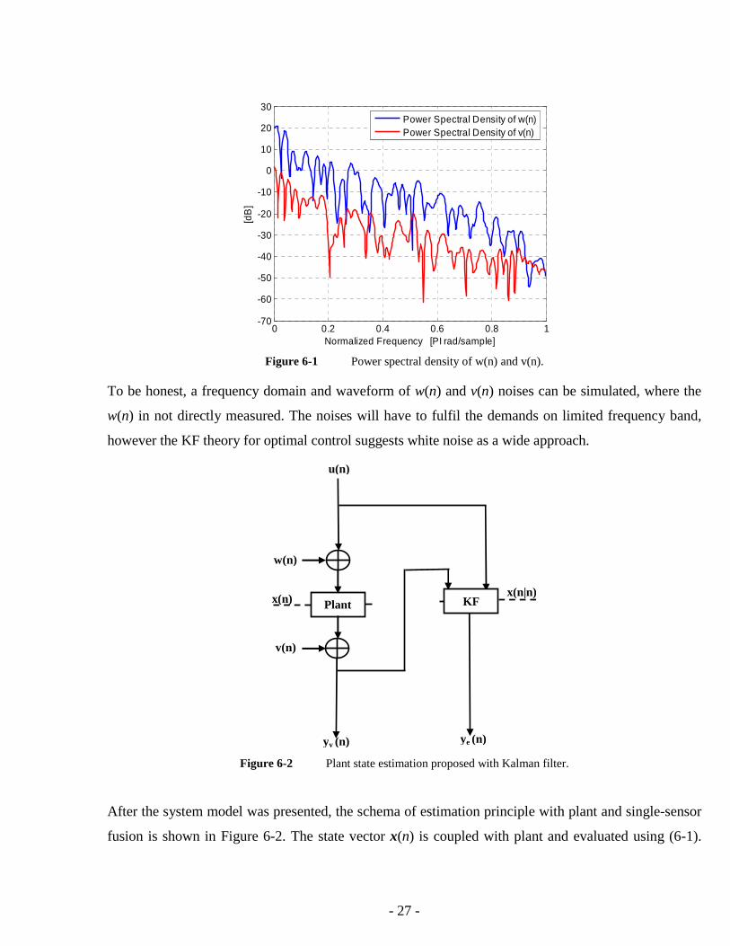
To be honest, a frequency domain and waveform of w(n) and v(n) noises can be simulated, where the

w(n) in not directly measured. The noises will have to fulfil the demands on limited frequency band,

however the KF theory for optimal control suggests white noise as a wide approach.

After the system model was presented, the schema of estimation principle with plant and single-sensor

fusion is shown in Figure 6-2. The state vector x(n) is coupled with plant and evaluated using (6-1).

0 0.2 0.4 0.6 0.8 1-70

-60

-50

-40

-30

-20

-10

0

10

20

30

Normalized Frequency [PI rad/sample]

[dB

]

Power Spectral Density of w(n)Power Spectral Density of v(n)

Figure 6-1 Power spectral density of w(n) and v(n).

Figure 6-2 Plant state estimation proposed with Kalman filter.

x(n|n) x(n)

yv (n) ye (n)

KF Plant

w(n)

v(n)

u(n)

- 28 -

The state estimation noted by x(n|n) is only processed in the block of KF. The process noise such as an

uncertainty is used in (6-1) and sensor noise model occurs in (6-2) of time-invariant system model. The

sensor noise is also called the observation noise, yv(n) is plant output, and ye(n) is filtered KF output.

Let us define the input control signal u(n) sinus wave below:

( ) ⎟⎠⎞

⎜⎝⎛=

50

2sin

nnu

π . (6-5)

Following formula is given for calculation a mean square error MSE. In order to evaluate the KF

performance, the MSE factor will be used to measure state estimation accuracy.

( )[ ] ( )[ ]{ }22 nΕnΕMSE aa −= (6-6)

The substituted variable a(n) will be applied in an experimental study and results the formula (6-7),

where a total number of summarised items can be of course either than 101 which will be stated.

( ) ( )∑=

100

0n

T nn xx101

1 (6-7)

The Figure 6-1 shows the option of high power of Q (6-3), while R stands unchanged (6-4) in thesis.

The system model (6-1)-(6-2) and the principle carry out in Figure (6-2) are used up to Unit 11.

The noise streams and their variances (6-3), (6-4) and MSE formula (6-6) will be used along with next

simulations up to Unit 14. In order to make multi-sensor fusion, many uncorrelated sensor noise

streams should be used in a sensor model but variances of each of them remain still the same regarding

to (6-4) up to the end of this thesis.

The input control signal (6-5) would be also used in further up to the Unit 12.

In this unit, our concern tends to find a mathematical identity and numerical similarity between CoKF

models in some tests. We are focusing on three CoKF models called Model 1-3 of KF taken from

the Unit 2. These models shown in Table 2-1 to 2-3 give their own filter observations called ye1(n),

ye2(n), ye3(n), respectively only in tests of this unit. First two models give their own state estimations

called x1(n|n) and x2(n|n), respectively. Last two models called Model 2 of KF and Model 3 of KF are

mathematically derived from and based on equations of the first Model 1 of KF, hence all of them

should be mathematically identical. To confirm this, they will be submitted in some tests.

State estimation accuracy will proceed in next steps as a function of process noise in examination on

Kalman filtering.

- 29 -

Test for MSE of difference between n)|(n1x and n)|(n2x . In this sub-test the MSE is shown

in Table 6.1. The difference between state estimates done in first two models is measured optionally

with low power of process noise and assigned to ( ) ( ) ( )[ ]n|n-n|n n 21 xxa = .

Test for MSE of difference between x(n) - n)|(n1x and n)|(n2x . The aim is to measure a

signal difference between expecting state and estimated one. Hence the evaluation criteria is

( ) ( ) ( )[ ]n|n- 1xxa nn = . The MSE for first model is shown in table.

The accuracy of state estimation of first model is high because MSE is equal to 1.284x10-4 and MSE for

second model is quite same with small difference about 10-10. Some values of x(n), x1(n|n) and x2(n|n)

are presented below to complete Table 6.2.

Either both models perform with numerical small error presented by Tables 6.1, 6.2 and high accuracy

of state estimation. Therefore the time n = 2 was chosen for Table 6.3 to make values unlike and

visible with three decimal points as much as possible. The states x1(n|n) and x2(n|n) tend to x(n) in the

worst case at the beginning of simulation when time n = 2, otherwise x1(n|n) and x2(n|n) are same.

Test for MSE of difference between observations. Here ye3(n) and yv(n) should be correlated

with up to unwanted sensor noise, where variance of a difference between them is equal to

2.49x10-4 and getting numerically close to 3.669x10-4 variance of sensor noise. The differences between

first two models and the third model are about 10-9 and 10-7, respectively.

Power of state x(n) of Plant 132.5

(MSE of [x1(n|n)]-x2(n|n)]) / (Power of x(n)) 8.5 . 10-14

Table 6.1 Test of state estimation of Model 1 and 2 of KF.

Power of state x(n) of Plant 132.5

(MSE of [x(n)]-x1(n|n)]) / (Power of x(n)) 1.284 . 10-4

Table 6.2 Test of state estimation of Model 1 of KF.

x(n) of Plant [1.122; 1.733; 1.520] . 10-3

x1(n|n) of Model 1 of CoKF [3.157; 0.075; 3.190] . 10-3

x2(n|n) of Model 2 of CoKF [3.159; 0.076; 3.190] . 10-3

Table 6.3 Estimated state vectors of Model 1 and 2 of KF and plant at time n = 2.

- 30 -

Moreover, the system model defined by (6-1) and (6-2) is presented in [5], and there the Q, R are equal

to one for w(n) and v(n) random noises, and ⎟⎠⎞

⎜⎝⎛=

5sin)(

nnu . We do not measure MSE of state estimates

in the case of Model 3 of KF, because this model does not estimate x(n|n) but it does

x(n|n-1) only. Hence plotted ye(n) outputs are shown in Appendix A.1 corresponding to identical figure

of first model in [5].

6.1 Conclusions

The Table 6.1 presents very small relative MSEs of Model 1-3 of KF. It means that all

equations of the Unit 2 and the improvement of Section 2.1 are useful.

Small difference, 8.5x10-14 in Table 6.1, between Model 1 and 2 of KF occurs due to singularity

avoided by the needed method presented in Section 2.1.

High state estimation accuracy is presented with small relative MSE, 1.284x10-4 in Table 6.2, in case of

Model 1 and 2 of KF. Also in Table 6.3, the values of state vectors are shown at time n = 2. There the

estimated states tend to state vector of plant numerically with small error. Assuming the periods of

time when 2>n , state estimation accuracy of a KF is so high that only high number of digits is

required to see any difference between states of plant and estimated states.

The third model shows figure of Appendix A.1 to be identical to one in [5]. The third model does not

produce state estimates but it does only the filtered output yv(n). There the filtered output of the third

model ye3(n) and observation yv(n) are correlated up to unwanted sensor noise v(n).

In a case of high power of process noise we can obtain similar conclusions. Measured relative MSE of

difference between x1(n|n) and x2(n|n) equals to 1.155x10-16 respecting the method presented above.

There the state estimation accuracy is high with small relative MSE (4.5x10-4) that corresponds to

Model 1 and 2 of KF for Table 6.2. A variance between observations of all three models is lower than

the previous case of low power of process noise.

As notice, to make relevant simulation the value of Q must be truly set to the variance of process noise.

Finally, high Q gathers the innovation KF gain M(n) resulting an amplified residuals r(n). So the

- 31 -

optimal feedback between a plant and estimator is established. In case of small power, the error in state

estimation yields 82% (3.669/4.5) out of power of w(n), and for high power the error of estimation is

about 0.35% (1.284x10-4 / 3.669 x10-2).

In this way, three models of the Unit 2 have been presented. They are mathematically derived

correctly and numerically performing state estimation with high accuracy with thanks to the

improvement presented in Section 2.1. This conclusion refers to the first solution in Section 1.3.

- 32 -

7 SIMULATION OF CENTRALIZED KALMAN FILTER

The aim of this unit is dedicated to verify CKF models built beyond MATLAB/Simulink. Two

Sections, 7.1 and 7.2, include some simulation results. This would satisfy the first question of

Section 1.1 with some successful Kalman filter models.

First, we specify system model by (6-1) and (6-2).

Referring back to the equations (6-3) and (6-4), certain matrices of w(n) and v(n) are used from the

Unit 6. In all simulations the only high power of w(n) noise is considered, view page 26.

Additionally the input signal u(n) is defined by (6-5) , where 10010n ...,,,= .

Then an evaluation of CKF models would be performed by MSE calculation with formula (6-6), where

( ) ( ) ( )n|n-nn xxa = . (7-1)

A relative MSE will be computed so that the MSE is divided by a state power of plant (6-7). For the

purpose of all simulations done up to Unit 11 the observation matrix can be given as follows:

⎥⎦

⎤⎢⎣

⎡=

001

001C . (7-2)

The Section 7.1 refers to a simple simulation of Model 1 to 3 of CKF. Prior to any usage, this

simulation will verify three models. After, when our CKF models are allowed for any use, they might

be implemented into real devices. The CKF models are tested to find all failures and model

imperfections even if any exist. The simulation is based on CoKF and CKF comparison, where two

sensors are assumed and their sensor noise streams are totally identical that does not occur in reality.

To be detailed, observation yv(n) is doubled for the reason of two nodes in CKF model. Hence this

situation can be only simulated. This way we will prove a CKF fusion and a performance of presented

equations in the Unit 3. Due to the fusion, a number of sensors should not change x(n|n) if all sensors

signals and particular noises are equal. So, we expect the state vector x(n|n) produced by CKF with two

sensors to be on an equality with x(n|n) of single sensor CoKF estimator, and also their equal filtered

ye(n) outputs. To make the fusion correct, we the ∑ - sum is displaced in material [15] by Е - mean.

The Section 7.2 refers to simulation with Model 1 to 3 of CKF containing two nodes. Although

there is no comparison between CoKF and CKF because two independent sensors are used in CKF

model, and their corresponding sensor noise streams are uncorrelated and zero-mean.

- 33 -

7.1 Testing the CKF fusion and performance

The CoKF model and CKF models are built according to equations of Table 2-1 and Tables 3-1

to 3-3, respectively. Same conditions for CoKF and CKF are used as in the Unit 6.

In Figure 7.1-1, the filtered outputs of CKFs and CoKF are overlapped without any difference. In other

words, the outputs of CKF and CoKF are the same quality and mathematically equivalent in this test.

Figure 7.1-2 Priori error variance CP(n|n-1)CT of filtered outputs in CKF and CoKF.

5 10 15 20 25 30 35 40 45 50 1

2

3

4

5

6

7

8 x 10 -3

Discrete Time [n]

CPCT

Priori error variance in MODEL 1 of KF, and MODEL 1 -3 of CKF

CPC' in Model 1 of KF CPC' in Model 1 of CKF CPC' in Model 2 of CKF CPC' in Model 3 of CKF

Figure 7.1-1 The CKF and KF observations of first output.

0 20 40 60 80 100 -2.5

-2

-1.5

-1

-0.5

0

0.5

1

1.5

2 Observations of KF, and Model 1 - 3 of CKF

Discrete Time [n]

Model 1 of KF Model 1 of CKF Model 2 of CKF Model 3 of CKF

- 34 -

The Figure 7.1-2 shows the priori error variance of filtered outputs computed by C P(n|n-1) CT. Finally,

all curves tend asymptotically to constant. On the basis of comparability with all models, the

covariance time update performs quite the same. One difference occurs at the discrete time n = 0 when

inverse covariance matrix is singular, but this defect is overcome by improvements presented in the

Sections 2.1 and 3.1. Then the singularity problem has no longer effect on state estimation

performance. In the case of CoKF estimator, the MSE is shown in Table 7.1-1 in second row and the

relative MSE in last one. The power of state x(n) is equal to 1.076.

SNR of State of Plant 14.83 dB MSE of CoKF 4.940 . 10-4 (MSE of CoKF) / (x(n) power of Plant) 4.593 . 10-4

The same MSE values are obtained for Model 1 and 2 of CKF. The first item presents the power of

state from a noiseless plant, which is divided over an extracted noise from the noisy plant state x(n).

This ratio is measured with decibel scale. A model of noiseless plant is created in our simulation but it

does not occur in a real system.

First model of CoKF and CKF is described by fundamental equations and fusion works correctly.

Those equations, as program controls, are listed in Table 2-1 and 3-1. The applied CKF fusion collects

nodal information of both nodes to be summarized into global information and divided by number of

sensors that equals to two. In order to present results of third CKF model, see Table 7.1-2 in below.

SNR of State of Plant 14.83 dB MSE of CKF 4.936 . 10-4 (MSE of CKF) / (x(n) power of Plant) 4.589 . 10-4

The Model 3 of CKF gives MSE about 4.936x10-4 and Table 7.1-1 of KF gives 4.94x10-4 of MSE.

Those values are getting numerically very close with the difference about 4x10-7. This is caused due to

a singularity problem in inverse covariance matrix calculation pending second iteration in this

simulation. The Model 3 of CKF includes three computations of inverse covariance matrix and the

Model 2 of CKF includes only two. Therefore, the Model 3 of CKF is computationally more demanded

than the previous Model 1 of KF called CoKF.

Table 7.1-1 MSE for Model 1 of KF.

Table 7.1-2 MSE for Model 3 of CKF.

- 35 -

7.2 Testing the CKF based on two sensors

In this section, we consider Model 1 to 3 of CKF but CoKF is not needed here. The aim is to

compare the Model 2 and 3 of CKF toward the Model 1 of CKF. The Model 3 of CKF is fully

centralized structure of KF and useful to solve the first question of Section 1.1 in Unit 8. Therefore it

will be submitted next test to confirm good CKF performance.

The Figure 7.2-2 shows the priori error variance CP(n|n-1)CT of filtered outputs. All curves tend to a

constant value. Additionally, the covariance time update performs comparably in all models. The state

error covariance matrix P(n|n-1) becomes singular during first two discrete times. The effect of

improvements can be seen in the beginning of Figure 7.2-2. After that the matrix is computed correctly

and CP(n|n-1)CT becomes stable. The MSE of CKF models is computed in the same way with previous

section. First two models of CKF give the same MSE value as shown in Tables 7.2-1.


5 10 15 20 25 30 35 40 45 50 -2

0

2

4

6

8

10 x 10

-3

MODEL 1 -3 of CKF Measured priori error variance of CKF filtered outputs

Discrete Time [n]

CPC’

CPC’ -Model 1 of CKF CPC’ -Model 2 of CKF CPC’ -Model 3 of CKF

Figure 7.2-2 Priori error variance CP(n|n-1)CT of all three CKF models.


- 36 -

To notice the rule, a low MSE corresponds to high state estimation accuracy. The MSE of third model

in Table 7.2-2 yields very likely value to the MSE of first model in Table 7.2-1.


Small difference between them is caused by the complexity problem calculation of inverse covariance

matrix especially computed at time n = 1 and 2. The best way of how to show high accuracy of state

estimation directly is the demonstration of x(n|n) in CKF models at time n = 2, see Table 7.2-4 below.

x(n|n) of Model 1 of CKF [ 1.835; -1.685; -2.233] . 10-2 x(n|n) of Model 2 of CKF [ 1.835; -1.685; -2.233] . 10-2 x(n|n) of Model 3 of CKF [ 1.886; -9.775; -2.130] . 10-2

7.3 Conclusions

After two tests in Sections 7.1 and 7.2, the CKF models are recognised to be usable in reality.

In Section 7.1, the CKF models are designed correctly. There the fusion of all CKF models performs

the same state estimate with the regard to small error about 4x10-7. This model imperfection does not

affect state estimation at all. In Tables 3-1 to 3-3 the fusion is performed by the following information

sum ∑oN

1. This sum is implemented in some equations of CKF model. The Section 7.1 verifies the

reason of allowed total number of sensors oN to be used such as waiting factor in the fraction

denominator.

In Section 7.2, three CKF models perform numerically quite the same state estimation measured with

MSE about 3.7x10-4. The measured values of state vector elements get numerically very close to state

vector of plant x(n). The state estimation accuracy of CKF model was tested.

This conclusion joints with the importance of first solution in Section 1.3. The point of all Unit 7 is to

obtain well performing CKF model with its correct fusion referred to the Section 7.1.


Table 7.2-4 State vectors of CKF models at discrete time n = 2.

- 37 -

8 CENTRALIZED AND DECENTRALIZED KALMAN FILTER COMPARISON

In this unit we will dedicate the effort to explore identity between decentralized, DKF, and

centralized, CKF, Kalman filter which can be measured by mean square error MSE in state estimates in

an experimental simulation study. The MSE values of CKF and DKF models will be compared

although both models are derived mathematically, see [11]. Both models are created according to

Table 3-3 and 4-1 as a flow of control, and articles [9], [11-13]. The models consist of two nodes,

shown in Appendix C.1.

The vast constraints are remarked on page 28, see Unit 6. The matrix C is defined in (7-2). The time n

is running from 0 to 100 in MATLAB simulation. High power of w(n) is been recently applied, (6-3).

Additionally, a relative MSE of a difference between DKF and CKF state estimates x(n|n) is

shown at last row of the following table. The value in first row is related to difference between x(n)

and x(n|n) of CKF state estimates. The second item explains a relative MSE of DKF computed in such

way as the previous MSE in the first row.

Both values are very similar to satisfy the numerical identity among CKF and DKF. The error

comparison is not crucial in performance comparison of both estimators that is still to come.

To make relevant comparison on estimators is to compute a difference between state vectors x(n|n) of

DKF and CKF, see the last value. This relative MSE is about 103 times lower than the first two values.

Actually, this value is expected to be small, because the DKF and CKF provide mathematically equal

states. As an example, the Table 8-2 shows some sampled values of state vectors at n = 2.

Table 8-1 MSE of DKF; MSE of CKF; MSE of estimated state x(n|n) (DKF-CKF) comparison.

(MSE of Model 3 of CKF) / (x2(n) of Plant) 3.420 . 10

-4

(MSE of DKF) / (x2(n) of Plant) 3.416 . 10

-4

(DKF x(n|n) - Model 3 of CKF x(n|n))2

/ (x2(n) of Plant) 3.429 . 10

-7

Table 8-2 State vectors of Model 3 of CKF, DKF and plant at n = 2

x(n|n) of Model 3 of CKF [-1.457; -0.719; -0.061]x(n|n) of DKF [-1.457; -0.719; -0.061]x(n) of Plant [-1.471; -0.729; -0.057]

- 38 -

One can see no numerical difference in state elements of both estimators due to low precision. The last

item shows the x(n) of plant that is on numerical comparability with x(n|n) of CKF and DKF.

In our simulation, two sensors and two nodes of DKF estimator called DKF1 and DKF2 are shown. As

shown in the last item of Table 8.1, the relative MSE is measured in the case of DKF1 and DKF2 and

shown below in Table 8-3.

So, the DKF and CKF operate well despite very small difference measured in state estimates.

8.1 Conclusions

The first question of Section 1.1 is applied to this conclusion being answered below :

“Demonstrate state estimation identity of decentralized Kalman filter, DKF, and centralized Kalman

filter, CKF, in an experimental simulation study assuming uniform filter conditions.

What are differences?”

We have measured the relative MSE about 10-2 in state estimates of CKF and DKF. Measured MSE of

x(n|n) difference between DKF1, DKF2 and CKF is about 103 smaller than the value mentioned firstly.

These facts can be deeply clarified via in Table 8-1 and 8-3.

In the practical point, we can say that both estimators perform on the same state estimation despite the

unimportant difference in our MATLAB simulations. This fact is caused by a computational problem of

covariance matrix singularity that can be overcome using the improvements in Sections 3.1 and 4.1.

Said the improvements are needed however causing a little inconvenience as a numerical problem.

Without the improvements either the DKF or CKF can not start up, that usually gives a singularity

problem. This is certain constraint. Toward to the power of ( )nu and ( )n|nx from the Unit 6, the DKF

is designed so that this error 3.429x10-7 is negligible.

Here we have presented the answer of the first question given by Section 1.1. In the next tests

we should build upon the MATLAB based model of DKF. In our simulations all signals are broadcasted

without any unknown latency or transmission failure in multi-sensor fusion.

∑[(DKF1 x(n|n) - CKF x(n|n))2] / (x

2(n) of Plant) 3.429 .10

-7

∑[(DKF2 x(n|n) - CKF x(n|n))2] / (x

2(n) of Plant) 3.429 .10

-7

Table 8-3 DKF verification toward to CKF result based on stated measurement.

- 39 -

9 ONE BIASED SENSOR IN DKF MODEL

The aim of this unit is to make some experiments on DKF estimator that contains a sensor

affected by a bias. Then an error seen on such affected state estimation would be measured in

MATLAB. Thus a relation of a total number of sensors and MSE will be explored. The second question

asked for in Section 1.1 will be answered. The Appendix C.3 and C.4 shows MATLAB models.

To make consistent work with previous units, the system model must be taken over the Unit 6. One

possible selection is chosen when sensor noises, as v1(n); v2(n); etc., are uncorrelated, however their

observation covariance R(n) are equal, see (6-4). As a simulation, the stream of w(n) differs from the

observation noises due to another pseudo random code. The MSE is defined by (6-6), a(n) by (7-1).

This unit is composed of four sections including some experiments with DKF performed with

high and low power level of process noise, see (6.3). The first sensor noise is additively coupled with

noise v1(n) and an existed bias. The Figure 9-1 illustrates time behaviours of bias.

First two sections (9.1 and 9.2) deal with DKF model that contains two and five sensors, respectively.

One sensor is affected by constant bias over a time period of simulation. Following next two sections

solve a problem of linearly increased bias considering two and five sensors.

The level of constant bias equals to 10, and the linear bias increases from zero up to 20.2 during

simulation time, where 100010n ...,,,= .

0 200 400 600 800 1000 0

2

4

6

8

10

12

14

16

18

20

Discrete Time [n]

B I A S

P R OF I L E S

LINEAR BIAS CONSTANT BIAS

Plot of Bias Profiles: CONSTANT BIAS; LINEARLY INCREASED BIAS

- 40 -

9.1 Constant bias and two sensors in DKF model

A bias handling ability is identified by measuring the MSE of state estimation optionally with

two power levels of process noise mentioned in tables below.

The observations and filtered signals are shown in Figure 9.1-1. The setting of value in Q(n) must

correspond truly to covariance of w(n). If not so, the state estimation may be not optimal. Moreover as

we can see in the figure, the bias influence works against the optimal state estimation. Making the Q(n)

lower than the appropriate covariance of w(n), the state estimation gives low accuracy while the bias

impact on green curve is best. This way both terms can not be solved, therefore other useful technique

is needed, see Unit 12.

Constant Bias = 10MSE of DKF State Vector 1.014

Table 9.1-1 Two nodes decentralized Kalman filter result, high power of w(n).

Table 9.1-2 Two nodes decentralized Kalman filter result, low power of w(n)

Constant Bias = 10

MSE of DKF State Vector 4.312 . 10-2

0 100 200 300 400 500 600 700 800 900 1000 -4

-2

0

2

4

6

8

10

12

14

Discrete Time [n]

Two Sensors Test Affected yv1(n) Uncorrupted yv1 (n) of Plant ye1(n) in high power of w(n) ye1(n) in low power of w(n)

Figure 9.1-1 Observations in DKF model of constant bias.

- 41 -

9.2 Constant bias and five sensors in DKF model

This experiment is related to the one presented in Section 9.1 but five sensors are taken. Here

the C matrix has the size of [5x3] with all rows been the same as in (7-2).

Here the goal is to find a relation of MSE and the total number of sensors in DKF model affected by

bias. We would like to compare the MSE2DKF of DKF model consist of two sensors, Table 9.1-1, and

five sensors MSE5DKF in the Table 9.2-1. Hence the MSE2DKF model is higher than MSE5DKF and their

ratio MSE / MSE 5DKF2DKF = 522526 .. = . The ratio of total number of sensors is 2.5, which gets

numerically near the computed value.

In MATLAB simulation with low power of w(n), the ratio is equal to 2.476 been near the ratio of total

number of sensors. The point is that the fusion in DKF model works as an averaging sum without any

intelligence as FDI, where the FDI method may be able to eliminate a sensor failure.

9.3 Linearly increased bias and two sensors in DKF model

Having one sensor affected by linearly increased bias, two test results will be presented here.

Constant Bias = 10


Table 9.2-1 Five nodes decentralized Kalman filter result, high power of w(n).

Table 9.2-2 Five nodes decentralized Kalman filter result, low power of w(n).

Constant Bias = 10


Linearly Increased BiasMSE of DKF State Vector 6.11

Table 9.3-1 Two sensors decentralized Kalman filter result, high power of w(n).

Linearly Increased BiasMSE of DKF State Vector 2.171

Table 9.3-2 Two sensors decentralized Kalman filter result, low power of w(n).

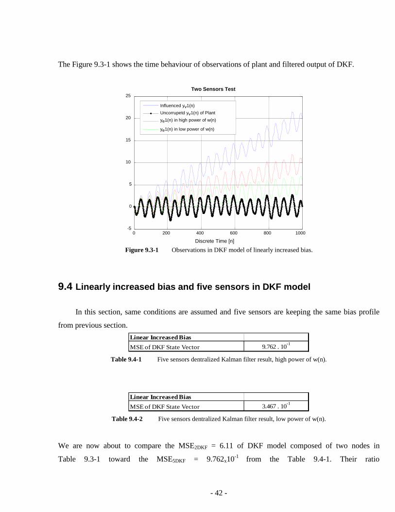
- 42 -

The Figure 9.3-1 shows the time behaviour of observations of plant and filtered output of DKF.

9.4 Linearly increased bias and five sensors in DKF model

In this section, same conditions are assumed and five sensors are keeping the same bias profile

from previous section.

We are now about to compare the MSE2DKF = 6.11 of DKF model composed of two nodes in

Table 9.3-1 toward the MSE5DKF = 9.762x10-1 from the Table 9.4-1. Their ratio

Linear Increased Bias


Table 9.4-1 Five sensors dentralized Kalman filter result, high power of w(n).

Linear Increased Bias


Table 9.4-2 Five sensors dentralized Kalman filter result, low power of w(n).

0 200 400 600 800 1000 -5

0

5

10

15

20

25

Discrete Time [n]

Two Sensors Test

Influenced yv1(n)

Uncorrupetd yv1(n) of Plant

ye1(n) in high power of w(n)

ye1(n) in low power of w(n)

Figure 9.3-1 Observations in DKF model of linearly increased bias.

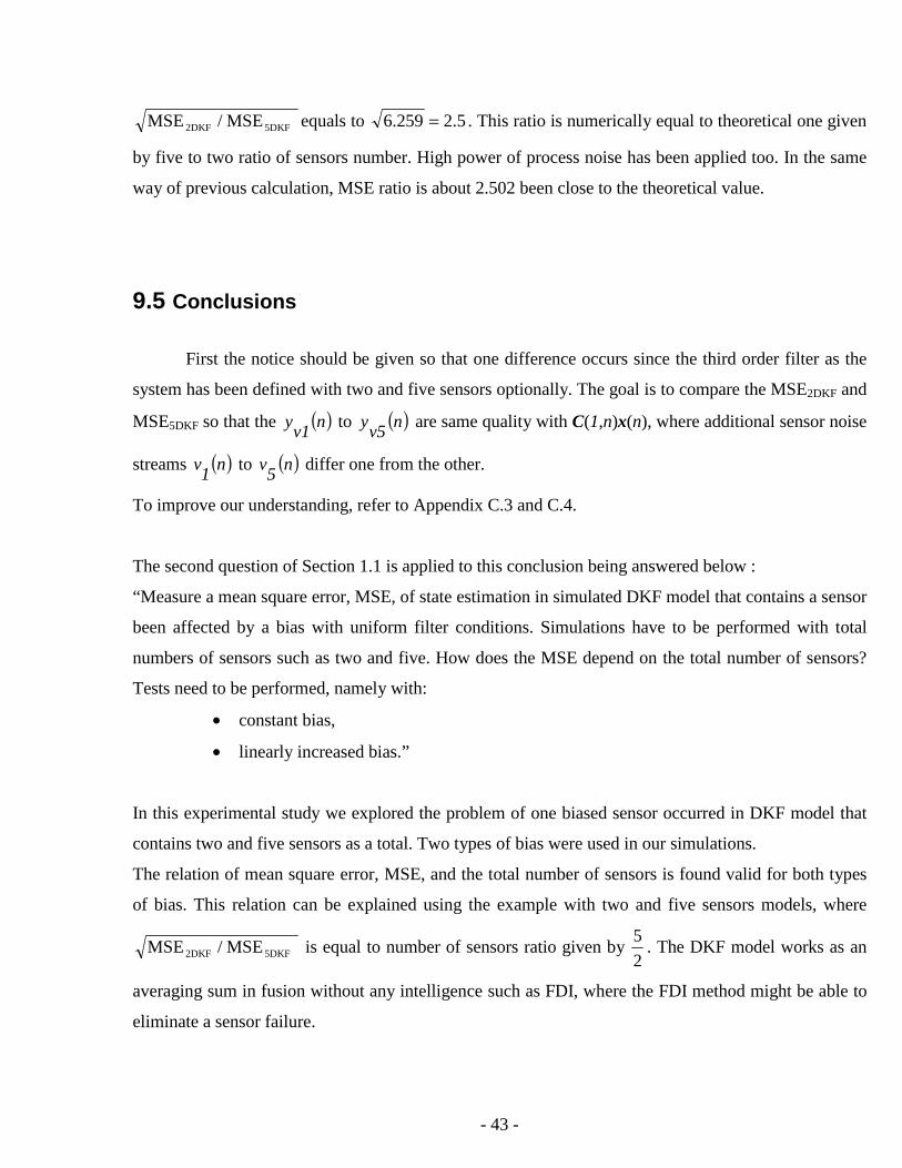
- 43 -

MSE / MSE 5DKF2DKF equals to 5.2259.6 = . This ratio is numerically equal to theoretical one given

by five to two ratio of sensors number. High power of process noise has been applied too. In the same

way of previous calculation, MSE ratio is about 2.502 been close to the theoretical value.

9.5 Conclusions

First the notice should be given so that one difference occurs since the third order filter as the

system has been defined with two and five sensors optionally. The goal is to compare the MSE2DKF and

MSE5DKF so that the ( )nv1

y to ( )nv5

y are same quality with C(1,n)x(n), where additional sensor noise

streams ( )n1

v to ( )n5

v differ one from the other.

To improve our understanding, refer to Appendix C.3 and C.4.

The second question of Section 1.1 is applied to this conclusion being answered below :

“Measure a mean square error, MSE, of state estimation in simulated DKF model that contains a sensor

been affected by a bias with uniform filter conditions. Simulations have to be performed with total

numbers of sensors such as two and five. How does the MSE depend on the total number of sensors?

Tests need to be performed, namely with:

• constant bias,

• linearly increased bias.”

In this experimental study we explored the problem of one biased sensor occurred in DKF model that

contains two and five sensors as a total. Two types of bias were used in our simulations.

The relation of mean square error, MSE, and the total number of sensors is found valid for both types

of bias. This relation can be explained using the example with two and five sensors models, where

MSE / MSE 5DKF2DKF is equal to number of sensors ratio given by 2

5. The DKF model works as an

averaging sum in fusion without any intelligence such as FDI, where the FDI method might be able to

eliminate a sensor failure.

- 44 -

The power of plant state was 1.25, power of constant bias was 100 and power of linearly

increased bias was 134. In other words, the power of bias was higher than the power of state. High

power of bias may cause catastrophic state estimation in Kalman-Filter estimation.

The 100-times big change of Q(n) makes:

• 23-times changed MSE for the test with constant bias (compare values in Table 9.1-1 and 9.1-2,

or Table 9.2-1 and 9.2-2);

• 2.8-times for the test with linear bias (Table 9.3-1 and 9.3-2, or Table 9.4-1 and 9.4-2);

Those MSE values differ due to the bias profiles, but the manner of bias time behaviour and effect on

state estimation or filtered output remains the same.

- 45 -

10 ONE BROKEN SENSOR IN DKF MODEL

The purpose of this Unit is to obtain a relation of MSE of state estimation measured in DKF

model and a total number of sensors. Only one sensor can be broken within total number of sensors. In

our model simulations a broken sensor provides zero value instead of its eventual correct filtered

output yv(n), where 100010n ...,,,= . This zero provided value is accepted by DKF estimator.

The model of DKF comprises of two and five sensors used in Sections 10.1 and 10.2,

respectively. In each section, two experiments are optionally performed with high and low power level

of process noise. The first section shows some results of a problem mentioned above, where two

sensors are associated with one system. The Section 10.2 presents some results with five sensors. Our

MATLAB models belong to Appendix C.3 and C.4. The DKF is developed according to Table 4.1.

The system dynamics is defined in Unit 6 where the C matrix takes the form of (7-2) or large size

as [5x2]. The MSE values and a(n) are computed according to formulas (6-6) and (7-1), respectively.

10.1 Testing the DKF with two sensors

This section presents two tables assuming different power levels of process noise noticed in

below the Tables 10.1-1 and 10.1-2. This experiment yields two sensors in DKF model.

Table 10.1-1 DKF result in two sensors test of broken sensor, high power of w(n).

Broken Sensor


Table 10.1-2 DKF result in two sensors test of broken sensor, low power of w(n).

Broken Sensor


- 46 -

10.2 Testing the DKF with five sensors

In the same way with previous section, the MSE is measured on five sensors system. We are

about to compare the MSE in Table 10.1-1 called MSE2DKF and MSE5DKF in Table 10.2-1.

There MSE2DKF is higher than MSE5DKF of five sensors model and their ratio

MSE / MSE 5DKF2DKF yields 496.2232.6 = . It is computed by the assumption of high power of w(n)

where its covariance is time-invariant. This ratio is numerically close to theoretical value given by 2

5

as the five to two ratio (a ratio of total number of sensors). This rule is valid also in a case of low

power of process noise with its covariance matrix Q, where the MSE / MSE 5DKF2DKF ratio

is 501.2256.6 = .

10.3 Conclusions

Below we apply the third question of Section 1.1 to this conclusion to be answered:

“Measure the MSE of state estimation in simulated DKF model that contains a broken sensor with

uniform filter conditions. Simulations have to be performed with two and five total numbers of sensors.

How does the MSE depend on the total number of sensors?”

The tested DKF model is composed of two and five sensors, where only first of them was broken.

Table 10.2-1 DKF result in five sensors test of broken sensor, high power of w(n).

Broken Sensor


Table 10.2-2 DKF result in five sensors test of broken sensor, low power of w(n).

Broken Sensor


- 47 -

The ratio MSE / MSE 5DKF2DKF equals to 2.496 and 2.501 assuming high and low power of process

noise, respectively. Both values are numerically near to the expected value 2.5. This value could not be

reached exactly because a power of sensor noise is not negligible and makes a small inaccuracy in

calculation, however all observations of sensors contain same power of sensor noise in our simulations.

From the measured MSE, noises are smoothed and a mean of them should be zero and any little mean

does not affect MSE calculation at all. A noise plays an important role in calculation mentioned above

because it is an unwanted random signal.

Comparing the values of MSE in experiments of corrupted sensor, Units 9 and 10, and correct sensor,

see Unit 6, here the value rapidly increased due to a failure of sensor.

The third question asked in Section 1.1 for finding the relation between MSE and the total number of

sensors is answered in this conclusion.

- 48 -

11 BY A DRIFT AFFECTED SENSOR IN DKF MODEL

This unit focuses on testing of estimators with sensors affected by a drift. All experiments

present decentralized Kalman filter, DKF, as an estimator in multi-sensor fusion. The main point of

corrupted system is to view an accuracy of state estimation as the opposite aspect of its measured mean

square error MSE. This way we like to find a relation between MSE and a total number of sensors

wherein only one of them would be affected by exponentially decreasing drift.

The DKF technique is implemented into all nodes of the decentralized structure simultaneously

performing estimation, see Unit 4. In a general way, at least one sensor in any node might be affected

by a drift. In all experiments of this unit, only first sensor is affected of which behaviour becomes

additionally a subject of our study. This sensor is simulated as a observations of plant multiplied by

drift varying from one down to zero. This type of sensor gives a fault in state estimation. The

remaining last sensors are drift-free sensors which provide correct observations to be accepted in the

structure of DKF.

Due to the drift, an optimal state of system may not be obtained. High state estimation accuracy

corresponds to a low MSE of state estimation performed by DKF. Here the tests are beyond a

simulation of DKF model that contains one, two and five sensors as the total number of sensors.

The drift problem in KF model with only one sensor is presented in Section 11.1. There we want

to see drift based approach to a basic problem in KF processing. The Model 1 of KF is used.

Next Sections 11.2 and 11.3 include DKF experiments with two and five sensors, respectively.

Two options of process noise power are used. Some simulated models shown in Appendix C.2 to C.4

are related to Section 11.1 to 11.3. All proposed MATLAB simulations are done in time periods of

1000...,,1,0=n ; the MSE formula is given by (6-6), where differential signal a(n) is given

by (7-1). As the assumption, variances of all sensor noises are equal but their noises are uncorrelated.

Process noise remains the same in all simulations with the kind of drift and input signal. The system

dynamics can be described as mentioned in the previous unit.

- 49 -

11.1 Kalman Filtering and drift in observations

First of all, it is needed to obtain some MSE measurements from the model of the drift. With

the given system model the (6-2) should be redefined to

( ) ( ) ( ) ( )nvnndnyv += Cx . (11.1)

This is a model of drifted sensor. Inside of the sensor, the drift might be not technically repaired

directly. The exponential drift d(n) can be defined as follows:

( ) eδn

nd Δ−−= ; 400Δ0 == ,δ . (11-2)

The drift slopes down starting the simulation when n = 0 and its exponent is determined by ∆ = 400.

The (11-2) formula is used starting with this unit up to the end of the thesis.

We start this experiment with low power of process noise in the system. In the case of KF with one

sensor (for CoKF), the effect on observations is shown in Figure 11.1-1. The filtered output ye(n) never

reaches wrong value of zero while impacted observation yv(n) does up to noise v(n). The drift gives

majority in error of state estimation but KF is not designed to cope with drift kind of errors. Thus drift

problem can not be solved by adjusting of Q matrix, hence this is related to Unit 12.

0 500 1000 1500 2000 -2

-1.5

-1

-0.5

0

0.5

1

1.5

2

Discrete Time [n]

-BLUE- yv(n) -RED- ye(n|n) in Model 1 of KF

Figure 11.1-1 Filtered output of CoKF and observations of plant, low of process noise.

- 50 -

Making the result viewable, the simulation is long. The Figure 11.1-2 shows some measured signals

optionally with high power of process noise. There the filtered output ye(n) of KF follows affected

plant observation yv(n) and curves of both signals are shown in Figure 11.1-2a.

The goal is also to get an experience in residual r(n) behaviour presented by curve of Figure 11.1-2b.

As an important fact, smoothed absolute value |r(n)| is correlated with the exponential drift shown in

black of Figure 11.1-2a. Normally high residual values tend to an error in state estimation. Then,

Figure 11.1-2c depicts the error variance between state of plant x(n) and estimator x(n|n). This variance

is being increased during the appearing drift and refers to MSE in Table 11.1-1 and Table 11.1-2.

Those tables present MSE of the same model assuming low power of process noise.

0 100 200 300 400 500 600 700 800 900 1000-2

-1

0

1

2

Discrete Time [n]

a)

0 100 200 300 400 500 600 700 800 900 1000-0.5

0

0.5

Discrete Time [n]

b)

0 100 200 300 400 500 600 700 800 900 10000

0.5

1

1.5

2

Discrete Time [n]

c)

var[x(n)-x(n|n)]

Residuals r(n)

Smoothed |r(n)|

Drift d(n)

Ye(n) of CoKF

Yv(n) of Plant

Figure 11-1.2 The examples of drift in system with one sensor. In a) ye(n) of Kalman filter and yv(n) of plant; b) influenced residuals r(n) in blue and smoothed | r(n)|; c) variance measured between expected x(n) state of plant and x(n|n) estimated state of Kalman filter.

- 51 -

11.2 Drift and two sensors in DKF model

In this section, DKF model contains two sensors and first of them is only affected by the drift.

Now we are allowed to compare some results of this and last section considering MSE values.

The MSE in Table 11.1-1 called MSE1KF equals to 6.618x10-1 and the MSE in Table 11.2-1 called

MSE2DKF equals to 1.659x10-1 and their ratio MSE / MSE 2DKF1KF is 997.1989.3 = . In similar way,

measured ratio of values in Table 11.1-2 and Table 11.2-2 gives 001.2004.4 = .

This section can be concluded in fact that these results are near the expected value equal to1

2 as a ratio

of total number of sensors. This small dissimilarity is caused by a little mean of noises w(n) and v(n).

Table 11.1-1 MSE of difference between plants and estimators state, high level of process noise.

Drift Impact

MSE of (CoKF State -Plant State) 6.618 . 10-1

Table 11.1-2 MSE of difference between plants and estimators state, low level of process noise.

Drift Impact

MSE of (CoKF State - Plant State) 2.572 . 10-1


Drift Impact

MSE of (DKF State - Plant State) 1.659 . 10-1


Drift Impact


- 52 -

11.3 Drift and five sensors in DKF model

In the same way with previous section, the MSE is measured and shown in following tables, but

the model employs five sensors.

We will compare MSE values of Sections 11.1 and 11.3. The MSE1KF equals to 6.618x10-1 and the

MSE of DKF model with five sensors called MSE5DKF equals to 2.686x10-2. Their ratio

MSE / MSE 5DKF1KF is 964.4639.24 = . In the case of low level of process noise, the ratio

gives 995.4947.24 = . Our results tend to expected ratio given by five because one and five sensors

have been taken into account with comparable quality in DKF model.

11.4 Conclusions

Below we apply the fourth question of section 1.1 to this conclusion to be answered:

“Measure the MSE of state estimation in DKF model that contains a sensor affected by a drift with

uniform filter conditions. Simulations have to be performed by using one, two, and five total numbers

of sensors. How does the MSE depend on the total number of sensors?”

As an approximation, the MSE is linearly proportional to the total number of sensors. For example

in our case of two sensors model, the estimator gives four times lower MSE of state estimation than

DKF with one sensor. Five sensors DKF provides 25-times lower MSE than the single sensor DKF.

The fourth question of finding the relation between MSE and total number of sensors has been

answered in this conclusion.


Drift Impact

MSE of (DKF State - Plant State) 1.031 .10-2


Drift Impact


- 53 -

12 FAULT DETECTION AND ISOLATION METHOD IN DECENTRALIZED KALMAN FILTERING

In Unit 11, we saw sensor drift problem that is expected to be solved by an additional system

able to detect a drift as a sensors fault. The drift gives a fault in state estimation. Hence this unit deals

with developing and simulating a traditional concept of fault detection and isolation, FDI, algorithm

used in MATLAB simulations, where a nodal structure of decentralized Kalman filter is assumed and

consist of three sensors/nodes. The FDI as an additional algorithm improves on DKF based structure to

avoid sensors’ failures. The DKF model with FDI system belongs to Appendix C.5.

Here the FDI algorithm would be used to detect a fault of an affecting sensor by an exponential drift

and consequently isolate it to minimise an error caused by the fault in state estimation. The algorithm

of FDI should be implemented in a self-acting technical system. The advantage of the algorithm is that

every node of the decentralized structure will be able to detect and isolate fault in sensor its self. As the

sensor information is propagated to all neighbouring nodes by a link interconnection, the FDI

algorithm is simultaneously performing fault detection in each node to improve robustness. It allows us

to implement the algorithm in a real time processing. The FDI technique is developed, [6], with an

inspiration of the fault-tolerant design, and correlation based detection used to reach middle accuracy

performance. Various techniques of fault detection for fault-tolerant design with diverse applications

are reported in [6]. We will present the reliability and some imperfections of FDI.

Starting this unit, a new model of linear finite-dimensional stochastic system dynamics is used

up to the end of this thesis as follows:

( ) ( ) ( ) ( )[ ] ( ) 0=+⎥⎥⎥

⎦

⎤

⎢⎢⎢

⎣

⎡

−+⎥⎥⎥

⎦

⎤

⎢⎢⎢

⎣

⎡−=+

−

−

−

−

0xxx ,nwnu

10.5.91

10.1.132

10.6.02

n

0010.6.907

102.33

012.633

1n2

1

2

1

, (12-1)

( )( )( )

( )( )( )( )⎥

⎥⎥

⎦

⎤

⎢⎢⎢

⎣

⎡+

⎥⎥⎥

⎦

⎤

⎢⎢⎢

⎣

⎡=

⎥⎥⎥

⎦

⎤

⎢⎢⎢

⎣

⎡

nv

nv

nv

n

100

010

001

ny

ny

ny

3

2

1

v3

v2

v1

x . (12-2)

- 54 -

In simulations the 4000...,,1,0=n . All noise description is taken over the Unit 6, excepting the

control input. A time response of the observations behaves as a third order of low pass filter, and all

observations yv1(n), yv2(n), yv3(n) give incomparable quality. Therefore the system model is technically

suitable for its property in next units too. The third order filter is suitable in navigations, where three

components such as a position, velocity and acceleration are estimated. Hence three components of

x(n) refer to three sensors.

Thus the uncorrupted system dynamics has been introduced but no fault of a sensor has been presented

yet. The equation (12-2) describes an ideal observations model without any fault.

After applying the drift problem, the fault in states will be solved in multi-state and multi-sensor DKF.

12.1 Testing the FDI implemented in DKF structure with one failed sensor

This section introduces the first example and the idea of FDI algorithm to be coupled with DKF

model. Throughout this and next section, the (12-1) is considered but the observation equation (12-2)

of stochastic model is omitted due to sensor fault and therefore a new realistic approach to the fault

coupled with first sensor is found as follows:

( )( )( )

( )( )

( )( )( )⎥

⎥⎥

⎦

⎤

⎢⎢⎢

⎣

⎡+

⎥⎥⎥

⎦

⎤

⎢⎢⎢

⎣

⎡=

⎥⎥⎥

⎦

⎤

⎢⎢⎢

⎣

⎡

nv

nv

nv

n

100

010

00nd

ny

ny

ny

3

2

11

v3

v2

v1

x , (12-3)

where d1(n) is defined by (11-2) with 1500=δ and 200=Δ . The delta δ describes the time when the

exponential drift starts. Next parameter Δ describes the slope on how quickly the drift turns down

inside of the first sensor.

We turn to observation processing of the first sensor because only this sensor is affected by the

exponential drift. The Figure 12.1-1 shows the observation yv1(n) and time behaviour of drift in black.

- 55 -

This drift effect provides a fault signal in residual depict in Figure 12.1-2. The red curve represents

smoothed absolute value ( )nr of residual (innovations sequence) produced in first node.

0 500 1000 1500 2000 2500 3000 3500 4000-1.5

-1

-0.5

0

0.5

1

1.5Residuals r(n) -BLUE-, Smoothed |r(n)| -RED-

Discrite Time [n]

Figure 12.1-2 Residuals in blue, and smoothed |r1(n)| in red.

0 500 1000 1500 2000 2500 3000 3500 4000-1.5

-1

-0.5

0

0.5

1

1.5First Impacted Sensor by Exponential Drift

Discrete Time [n]

Ye1(n) of PlantDrift Profile Exp[-|n-1500| / 200]

Figure 12.1-1 First corrupted sensor by exponential drift.

- 56 -

The estimators of second and third node have correct or a little noisy residuals r2(n) and r3(n). Signals

of r2(n) and r3(n) are expected to be not correlated with yv2(n) and yv3(n) respectively, when at least

another sensor is corrupted. The FDI algorithm attempts to reach zero moveable failure signal into the

residuals of neighbouring nodes (i = 1 and 2). All three residuals are expected to be processed by DKF

and FDI in a way to have a nominal, i.e. no-failure mode. In the absence of a failure, residuals should

be close to the observation noises. Three different residuals is referred to three nodes that can be found

as follows:

( ) ( ) ( )n|nnynr vii Cx−= , (12-4)

and coupled with the i-th sensor in i-th node, where i = 1, 2, 3. Each node includes its own processor

with DKF technique to perform state estimation in real time processing. The x(n|n) results on the same

in every node of decentralized structure either with or without any sensor failure. The FD and

consequential FI algorithms are applied in every processor to avoid or at least minimise a fault in state

estimation.

As it has been outlined, the FDI deals with two algorithms such as fault detection and fault isolation.

Both will be explored and simulated with comprehensive results in two parts below.

- 57 -

Fault detection. This part presents a general idea of the fault detection algorithm executed in every

processor of corresponded the i-th node. It indicates that a fault is recognised, see the flowchart below

as the timing diagram.

Fault Detection system inside of DKFi node

Decision Making (Reasoning)

( ) ( ) ( )

( )⎭⎬⎫

⎩⎨⎧ =

⎭⎬⎫

⎩⎨⎧ =

⎭⎬⎫

⎩⎨⎧ ≥

⎭⎬⎫

⎩⎨⎧ ≥

0nijBinaryCorr ELSE

1nijBinaryCorr THEN 0.05nijEnable AND 0.9nijNCorr IF (12-10)

NCorrij(n) is input BinaryCorrij(n) is output of this block

Preprocessing – Median Filter vs. Smoother

( ) ( ){ } ( ) ( ){ }1n|ninviyMEDIANni

rMEDIANni

Y −−== xC (12-5)

Causal Detection

( ) ( )kniY 0

1)j(Nkk1

jNijRS

jN

1nijCorr +∑

−−=⎟⎠⎞⎜

⎝⎛ +−= (12-6)

( )( ) ( )[ ] ( )

( )[ ] ( )⎥⎦⎤

⎢⎣⎡

⎥⎦⎤

⎢⎣⎡−

=nijRSσ niYσ

nijRSΕ niYΕnijCorrnijNCorr (12-7)

, where Reference Signals definition follows:

( )⎪⎩

⎪⎨

⎧

==−

==−

=1000...,1,0,k2,j,e300

k500...,1,0,k1,j,e100

k

kijRS (12-8)

Evaluation of Causal Detection

( )( )

( )[ ]j

1n|nxiCσ

nijCorrnijEnable

−= (12-9)

Pulse Prolonging Procedure for Preventing the Post-Exitation

( )

{ }On Holdor Clear ELSE

samples j

Nby pulse Prolong THEN falled nij

BinaryCorr IF⎭⎬⎫

⎩⎨⎧

⎭⎬⎫

⎩⎨⎧

(12-11)

BinaryCorrij(n) is modified at the output of this block

Table 12.1-1 The timing diagram of fault algorithm inside of DKFi processor in an i-th node, where ri(n) is

a residual and Cix(n|n-1) are inputs of FDI system; and BinaryCorrij(n) is one output.

- 58 -

The fault detection algorithm can be divided in two stages: residual generation and decision making.

1. In the first stage, the residual (shown in Figure 12.1-2 of blue curve and given by (12-4)), and

the enhanced failure effect on the residual is called the fault signature (Figure 12.1-2 of red curve).

Thus this effect should be utilised in fault detection algorithm. The residuals are obtained from

observations using (12-4) in every node. As the example, after n = 1500 the appeared drift permanently

gives exponentially increasing huge signal )(1 nr depict in Figure 12.1-2. Then the absolute value

)(1 nr is smoothed by median filter and assigned to Y1(n), see (12-5) and [19].

Generally, median filter makes the smoothing as a low-pass filter. In every node, median filter takes 25

samples of )(nri signal into an overlapping block. In digital signal processing this block is called a

buffer of memory. Then these samples are reordered starting from their minimal value up to maximum

value and stored into a new block of reordered samples. Only the 13-th sample of the new block is

assigned to Yi(n).

2. In the second stage, the procedure of decision making is needed for fault detection to decide

whether a fault is presented or not in residuals. A spurious fault is not our objective of study.

The fault signature Y1(n) is correlated with real drift d1(n) been presented in Figure 12.1-1. This is the

eventual fact for fault detection. Here the problem is that real drift d1(n) is unknown for every

processor in a node. Thus a presumption of possible drift profiles should be made from some

previously done measurements or employed expert systems. Thus various drift models need to be

created and stored in memory of each processor such as reference signals (12-8). Actually, it is difficult

to exactly suppose any drift profile, so that the mathematical description of every reference signal may

differ from real drift d1(n) but high correlation between them still exits to be suitable in fault detection.

The point is that, the permanently stored reference signals and measured Y1(n) are correlated by

defining (12-6). Thus the cross-correlation (12-6) is high when a fault occurs because d1(n) is

contained in Y1(n) and yv1(n). This procedure is performed in every node separately. Two reference

signals RS11(k), RS12(k) are shown in Figure 12.1-3 and used in every node/processor.

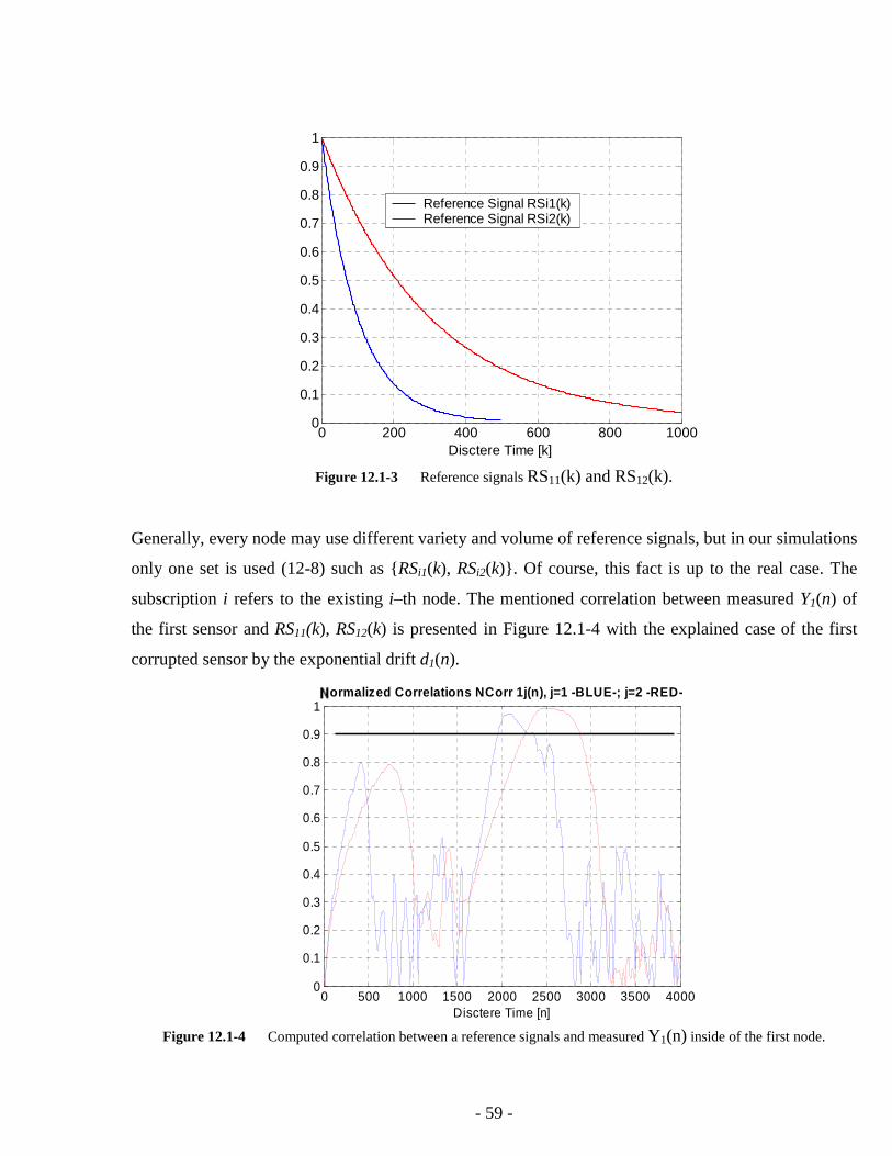
- 59 -

Generally, every node may use different variety and volume of reference signals, but in our simulations

only one set is used (12-8) such as {RSi1(k), RSi2(k)}. Of course, this fact is up to the real case. The

subscription i refers to the existing i–th node. The mentioned correlation between measured Y1(n) of

the first sensor and RS11(k), RS12(k) is presented in Figure 12.1-4 with the explained case of the first

corrupted sensor by the exponential drift d1(n).

Figure 12.1-3 Reference signals RS11(k) and RS12(k).

0 200 400 600 800 10000

0.1

0.2

0.3

0.4

0.5

0.6

0.7

0.8

0.9

1

Disctere Time [k]

Reference Signal RSi1(k)Reference Signal RSi2(k)

Figure 12.1-4 Computed correlation between a reference signals and measured Y1(n) inside of the first node.

0 500 1000 1500 2000 2500 3000 3500 40000

0.1

0.2

0.3

0.4

0.5

0.6

0.7

0.8

0.9

1Cormalized Correlations NCorr 1j(n), j=1 -BLUE-; j=2 -RED-

Disctere Time [n]

- 60 -

The blue curve corresponds to correlation NCorr11(n) (computed by (12-7) and (12-6)) between RS11(k)

and Y1(n). Finally, a fault caused by drift might be correctly detected only if some correlations

NCorr11(n) and NCorr12(n) crossed threshold equal to 0.9 (solid black line) in conjunction with

Enable11(n) and Enable12(n) 05.0≥ . This decision making is given by (12-10). The Enable11(n) and

Enable12(n) signals are found by (12-9) with i = 1 and j = 1 and 2 and both play an important role in the

avoidance of spurious detections possibly caused by a very small power of residuals.

Then two bitwise pulses are generated by BinaryCorr11(n) and BinaryCorr12(n) in Boolean algebra.

They are equal to one if valid fault has been detected, or zero if no fault has been detected. These two

pulses are prolonged by 500 and 1000 periods and updated by (12-11) and shown in Figure 12.1-5.

Both signals BinaryCorr11(n) and BinaryCorr12(n) would be logically combined by performing bitwise

logical OR operation to get a coupled pulse that starts at period of 1955 and ends at 3878. The process

of fault detection has been described by the example of decentralize structure containing three sensors

where the first of them accidentally failed.

0 500 1000 1500 2000 2500 3000 3500 4000

0

1

a)

0 500 1000 1500 2000 2500 3000 3500 4000

0

1

Discrete Time [n]b)

Figure 12.1-5 Two pulses after the fault detection: a) BinaryCorr11(n) pulse (fallen down at n = 2291) prolonged by 500 samples b) BinaryCorr12(n) pulse (fallen down at n = 2878) prolonged by 1000 samples.

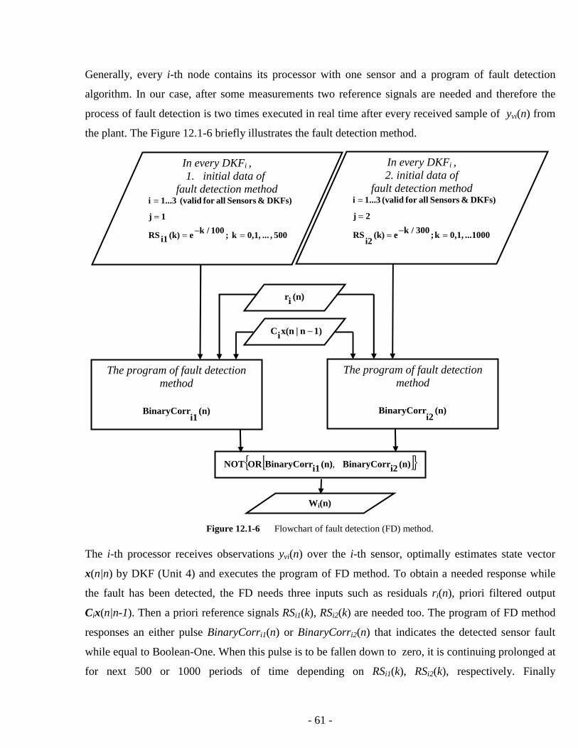
- 61 -

Generally, every i-th node contains its processor with one sensor and a program of fault detection

algorithm. In our case, after some measurements two reference signals are needed and therefore the

process of fault detection is two times executed in real time after every received sample of yvi(n) from

the plant. The Figure 12.1-6 briefly illustrates the fault detection method.

The i-th processor receives observations yvi(n) over the i-th sensor, optimally estimates state vector

x(n|n) by DKF (Unit 4) and executes the program of FD method. To obtain a needed response while

the fault has been detected, the FD needs three inputs such as residuals ri(n), priori filtered output

Cix(n|n-1). Then a priori reference signals RSi1(k), RSi2(k) are needed too. The program of FD method

responses an either pulse BinaryCorri1(n) or BinaryCorri2(n) that indicates the detected sensor fault

while equal to Boolean-One. When this pulse is to be fallen down to zero, it is continuing prolonged at

for next 500 or 1000 periods of time depending on RSi1(k), RSi2(k), respectively. Finally

The program of fault detection method

(n)

i1BinaryCorr

The program of fault detection method

(n)

i2BinaryCorr

In every DKFi , 1. initial data of

fault detection method

500 , ... 0,1,k ;100 /ke(k)i1RS

1j

DKFs) & Sensors allfor (valid 1...3i

=−=

=

=

In every DKFi , 2. initial data of

fault detection method

...1000 0,1,k ;300 /ke(k)i2

RS

2j

DKFs) & Sensors allfor (valid 1...3i

=−=

=

=

(n)ir

1)n|x(niC −

[ ]{ }(n)i2BinaryCorr(n)i1BinaryCorrORNOT ,

Wi(n)

Figure 12.1-6 Flowchart of fault detection (FD) method.

- 62 -

BinaryCorri1(n) and BinaryCorri2(n) are logically combined by OR to get a coupled pulse been one’s

complemented (negated) after to get the weighting factor Wi(n). The Wi(n) are common members

between presented fault detection and fault isolation method.

Fault isolation. This part presents the FI algorithm to the important theme of sensor validation in

decentralized structure in multi-sensor fusion. Of course generally, a major number of sensors can be

affected by a drift at the same time.

The main focus on fault isolation is based on variance error information VEIi(n) and state error

information SEIi(n) validation. These two matrices are usually corrupted by a fault while the i-th

sensor is affected by a drift. During successful fault detection, the corrupted VEIi(n) and SEIi(n)

matrices would be isolated only by the node wherein its corresponding sensor has been found incorrect

by FD program implemented inside of a corresponding node. The Wi(n) results two instances as

⎩⎨⎧

=detectedfault nowhen ,1

detectedfault when ,0)(nWi . (12-12)

In DKF estimator of every node the VEIi(n) and SEIi(n) are replaced by the matrix multiplications

( ) ( )nnW ii VEI , (12-13)

and

( ) ( )nnW ii SEI (12-14)

, respectively.

This procedure will be shown in Figure 12.1-7. In other words, this weighting factor Wi(n) is found to

cross the VEIi(n) and SEIi(n) matrices using (12-13) and (12-14).

- 63 -

Every block of processor is denoted by DKFi+FD. An outage part of Figure 12.1-7 performs the fault

isolation according to (12-13) and (12-14). Thus the FI crosses matrices VEIi(n), SEIi(n) via the

weighting factor Wi(n) when necessary. Then a number of correctly performing sensors is lower than

the total number of sensors if a failure occurs.

Hence the number of correctly performing sensors can be computed as follows:

∑=

=3

1

)(i

i nWN , (12-15)

C3 ye3(n)=C3x(n|n) yv3(n) x(n|n) A, B, Q, R, u(n) Global SEI(n) SEI3(n) N NON-FD3(n) Global VEI(n) VEI3(n)

DKF3 +FD


DKF2 +FD


DKF1 +FD

W1(n) SEI1(n)

W1(n)

W1(n) VEI1(n)

W2(n) SEI2(n)

W2(n)

W2(n) VEI2(n)

W3(n) SEI3(n)

W3(n)

W3(n) VEI3(n)

∑=

3

1i(n)

i(n)SEI

iW

∑=

3

1i(n)

iW

∑=

3

1i(n)

i(n)VEI

iW

÷ ×

× ÷

n.o.correct sensors

∑=

3

1i(n)

i(n)SEI

iW

∑=

3

1i(n)

iW

∑=

3

1i(n)

i(n)VEI

iW

÷ ×

× ÷

n.o.correct sensors

∑=

3

1i(n)

i(n)SEI

iW

∑=

3

1i(n)

iW

∑=

3

1i(n)

i(n)VEI

iW

÷ ×

× ÷

n.o.correct sensors

Link Interconnection

Figure 12.1-7 DKF with fault detection system inside and isolation system around.

- 64 -

where we have three sensors totally in our simulations. These data of (12-13) – (12-15) are broadcasted

through the link interconnection and known at receivers part of every node in Figure 12.1-7. Finally,

equations (4-10) and (4-11) are employed with whole fusion, state estimation, and correct fault

isolation. The remaining inputs and outputs presented in Figure 12.1-7 are used only in estimation. The

executed FDI algorithm has some shown test results below.

Testing the DKF, which contains low power level of process noise and one failed

sensor in decentralized structure of multi-sensor fusion. The FDI performance of weights

from W1(n) to W3(n) and the number of correct sensors N are demonstrated in Figure 12.1-8 below.

This example shows the functionality of estimator with FDI method containing three sensors in DKF

structure. Low power level of process noise (6-3) is used in this test, and first sensor fails starting at

0 500 1000 1500 2000 2500 3000 3500 40000

1

The

Wei

ght

W1

a)

0 500 1000 1500 2000 2500 3000 3500 40000

1

The

Wei

ght

W2

b)

0 500 1000 1500 2000 2500 3000 3500 40000

1

The

Wei

ght

W3

c)

0 500 1000 1500 2000 2500 3000 3500 40000

1

2

3

Discrete Time [n]

Sum

of a

llW

eigh

ts

d)

Figure 12.1-8 The performance of fault detection system depicted by: a) plotted weight W1(n) b) plotted weight W2(n) c) plotted weight W3(n) d) the sum of all weights equal to the number of correct sensors N.

- 65 -

n = 1500 and finishing by n = 4000. The first node detects the fault of its own sensor with the FDI

method during the detection term when n = 1955 … 3878, see Figure 12.1-8. The isolation of the

sensors fault is expected immediately when it starts, but our FDI method needs about 500 periods to

decide if the fault has occurred similar to drift profile (compared to reference signals (12-8) in

processors memory). This reliability of system detection refers to correlation function performance

with corresponding products NCorr11(n), NCorr12(n), threshold equal to 0.9, see (12-10), and

prolonged pulses BinaryCorr11(n), BinaryCorr12(n) produced by the first node/sensor. The next two

weights remain unchanged due to second and third sensors re correct.

In all sections of FDI tests, we like to specify the related MSE of state estimation. At first, it is

needed to remark on the state vector of plant x(n) and the estimated state vector x(n|n) of the model

with FDI method seen in Figure 12.1-7. Their difference a(n) is given by (7-1), and the mean square

error, MSE, of the state estimation is computed using (6-6) formula. The accuracy of state estimation is

measured by MSE in proportion to power of plant state, called relative MSE. This power is given by:

( ) ( )∑=

4000

0n

T nn4001

1xx , (12-16)

where 4000...,,1,0=n during MATLAB simulation. This relative 99.96% MSE is measured when

all sensors have worked without any fault at 1500...,,1,0=n ; and it is presented in Table 12.1-2.

A new criteria needs to be specified to evaluate a reliability of parallel DKF structure with FDI. At the

periods 4000...,,1502,1501=n during the failure, the reliability is found:

( ) ( )

( ) ( )n|nn

n|nn

|MSE

|MSE1 FDI

xx

xx

−

−− . (12-17)

The ( )n|nFDI

x is a state vector managed by the Figure 12.1-7 and ( )n|nx is a fully corrupted state

vector without FDI. Thus ( )na is conditionally defined in fraction of (12-17). This fraction determines

how much energy needs to compensated in states more, but there is nothing to do with state estimation

accuracy. This test gives about 75% FDI reliability in Table 12.1-2.

The accuracy of state estimation The reliability of FDIin the structure of DKF in the structure of DKF

during <0; 1500> during <1501; 4000>

9.996 . 10-1 7.460 . 10-1

Table 12.1-2 Related MSE of state estimation, and the reliability of FDI technique.

- 66 -

Testing the DKF, which contains high power level of process noise and one failed

sensor in decentralized structure of multi-sensor fusion. In this part, we demonstrate the

performance of previous system with 100-times higher power level of process noise. Here the

reliability is about 70% and almost 5% lower than the obtained one from the previous case of a little

process noise, see Table 12.1-3. Illustrated signals are additionally shown in Figure 12.1-9.

0 500 1000 1500 2000 2500 3000 3500 40000

0.5

1

Drif

t P

rofil

e

a)

0 500 1000 1500 2000 2500 3000 3500 4000

-1

0

1

DK

F w

ith/w

ithou

t F

DI

b)

0 500 1000 1500 2000 2500 3000 3500 40000

0.05

0.1

0.15

0.2

P(n

)

c)Discrete Time [n]

Figure 12.1-9 Plotted signals of DKF system with FDI conditionally with low power level of process noise: a) the profile of drift at the first sensor, b) the observation yv1(n) of the first sensor in GREEN; filtered output ye1(n) of DKF with FDI

in RED; signal of pure filtered output of DKF without any FDI plotted by BLUE color, c) state error variance measured at DKF estimation of the system with FDI technique.


during <0; 1500> during <1501; 4000>

9.990 . 10-1 6.966 . 10-1


- 67 -

The FDI detects the failure at periods between 1953 and 3652, and consequently isolates the sensor

fault however the drift occurs between 1501 and 4000 as known in Unit 12. The state estimation

accuracy is high when no drift appears.

The first Figure 12.1-9a demonstrates profile of the exponential drift mentioned above and known such

as the sensors fault. There we can see the red curve of compensated power done by the FDI method.

The Figure 12.1-9c demonstrates the state error variance ( )[ ]nvar a , where ( ) ( ) ( )n|nnFDI

n xxa −= . The

variance is highly produced during the term about the times 1500 to 2000, when the fault detection is

in the process and the state estimation is corrupted. Also a high error is produced at the state estimation

from the time 3653 until the end of simulation due to unregonisable drift in residuals.

12.2 Testing the FDI implemented in DKF structure with two failed

sensors

This section deals with the same example as previous one, but the first two sensors are affected

by two different drifts and one sensor remains correctly doing. The observations model is defined as:

( )( )( )

( )( )

( )( )( )⎥

⎥⎥

⎦

⎤

⎢⎢⎢

⎣

⎡+

⎥⎥⎥

⎦

⎤

⎢⎢⎢

⎣

⎡=

⎥⎥⎥

⎦

⎤

⎢⎢⎢

⎣

⎡

nv

nv

nv

(n)

100

0nd0

00nd

ny

ny

ny

3

2

11

v3

v2

v1

x , (12-18)

where the time 4000...,,1,0=n remains unchanged in simulation. The drift d1(n) is taken over the

Section 12.1, and the slow d(n) is defined by (11-2) with 1500=δ and from the Unit 11. The powers of

sensor noises are defined by (6-4). The time behaviours of the drifts are shown in below.

Figure 12.2-1 Drifts d1(n) and d(n).

- 68 -

Testing the DKF, which contains low power level of process noise and two failed

sensors in decentralized structure of multi-sensor fusion. The state estimation accuracy

remains still the same when no failure has been caused by sensors at 1500...,,1,0=n . Although the

reliability of FDI method is about 14% higher than presented one in Section 12.1, because signals of

first two sensors are not the same quality. These facts refer to table below.

The FDI performance in weights W1(n) to W3(n) and the number of correct sensors N are demonstrated

in Figure 12.2-2. There the weights W1(n) and W2(n) fall down when sensors faults have been detected.

The third remaining sensor is not corrupted, which fact corresponds to the weight W3(n) that ensures

fully transmitted VEI3(n) and SEI3(n) over the link interconnection. The Figure 12.2-2c illustrates the

number of correct sensors obtained by the applied sum (12-15) of W1(n) to W3(n).

0 500 1000 1500 2000 2500 3000 3500 40000

0.5

1

The

Wei

ght

W1

a)

0 500 1000 1500 2000 2500 3000 3500 40000

0.5

1

The

Wei

ght

W2

b)

0 500 1000 1500 2000 2500 3000 3500 40000

0.5

1

The

Wei

ght

W3

c)

0 500 1000 1500 2000 2500 3000 3500 40000

1

2

3

Discrete Time [n]

Sum

of

all

Wei

ghts

d)

The Weight of the 1-st Impacted Sensor

The Weight of the 2-nd Impacted Sensor

The Weight of the 3-rd Impacted Sensor

The Number of NonImpacted (active) Sensors

Figure 12.2-2 The performance of fault detection system depicted by: e) plotted weight W1(n) f) plotted weight W2(n) g) plotted weight W3(n) h) the sum of all weights equal to the number of correct sensors N.


during <0; 1500> during <1501; 4000>

9.996 . 10-1 8.894 . 10-1


- 69 -

0 500 1000 1500 2000 2500 3000 3500 4000

0

0.5

1

The

Wei

ght

W1

a)

0 500 1000 1500 2000 2500 3000 3500 4000

0

0.5

1

The

Wei

ght

W2

b)

0 500 1000 1500 2000 2500 3000 3500 4000

0

0.5

1

The

Wei

ght

W3

c)

0 500 1000 1500 2000 2500 3000 3500 40000

1

2

3

Discrete Time [n]

Sum

of

all

Wei

ghts

d)

The Weight of the 1-st Impacted Sensor

The Weight of the 2-nd Impacted Sensor

The Weight of the 3-rd Sensor

Number of NonImpacted (active) Sensors

Figure 12.2-3 The DKF system with FDI and its functionality under high power of process noise: i) plotted weight W1(n) j) plotted weight W2(n) k) plotted weight W3(n) l) the sum of all weights equal to the number of correct sensors N.

Testing the DKF, which contains high power level of process noise and two failed

sensors in decentralized structure of multi-sensor fusion. Here the FDI reliability is smallest

of all, abut only 54%, and shown below in table. High power of process noise affects the functionality

of FDI system. This fact is encountered with spurious detection of fault in seldom fallen weight W3(n).

This is the imperfection of FDI simply basing on cross-correlation function. One can say that this is the

limit that the FDI algorithm refuses to work and the DKF is not under control.

In Figure 12.2-3, we can see two short periods (2100-2650 and 3550-4000 approximately) when the

DKF works without any control and Q(n) and R(n)are substituted by some small defaulted values.


during <0; 1500> during <1501; 4000>

9.990 . 10-1 5.388 . 10-1

Table 12.2-2 Related MSE of state estimation, and the reliability of FDI technique, with high power of w(n).

- 70 -

12.3 Conclusions

Below we apply the fifth question of section 1.1 to this conclusion to be answered:

“Find out a fault detection and isolation, FDI, algorithm been possibly useable for DKF model. This

model has to be tested with a minor number of affected sensors by exponentially descending drifts.

What is a performance of this DKF model with applied FDI algorithm, when:

• one sensor is affected by the drift, and additionally two sensors are correct;

• two sensors are affected by two miscellaneous drifts, plus one correct sensor?”

The major requirement on this fault detection and isolation, FDI, algorithm is an availability to

multiple observations. We have shown on how to apply FDI algorithm to the problem of faults in

sensors. The FDI algorithm has been found out in three strategies:

1. exercising on fault detection method, FD

2. exercising on fault isolation method, FI.

The all algorithm is tailor-made on system dynamics and the knowledge of drift in sensors.

Firstly the question related to one affected sensor will be answered below. Our simulation

results show that the DKF model with FDI algorithm yields 75% reliability of FDI performance

insomuch that a pure DKF model without FDI provides exactly 0% reliability. The FDI reliability is

not meant to be state estimation accuracy, although its relative MSE is about 0.01. In case of high

process noise, results of simulations show about 70% reliability of FDI algorithm. The five percentage

aggravation is caused by 100-times higher power of process noise, where the

cross-correlation function used in FDI system is disturbed by that.

Having two sensors affected by exponential drifts, the FDI reliability rises up to 84% which

describes the benefit of FDI. But considering 100-times higher power of process noise, the reliability is

reduced down to 54%, and relative MSE of state estimation is about 0.11. This is the FDI imperfection

with major number of corrupted sensors. Two failed sensors out of three total sensors and having high

power of process noise result in loss of performance of FDI. So said, the FDI functionality is correct as

long as a number of affected sensors is minor otherwise the DKF may be at risk.

- 71 -

The reliability of FDI describes on how much lost energy in ( )n|nx is compensated back rather than

the pure DKF without FDI can not perform.

The answer of fault detection and isolation algorithm has been recently given above.

Simulation conditions:

The DKF models use multi-state; multi-sensor system fusion with different quality of observations.

Time behaviour of u(n) is sinus as a still oscillated signal rather used than a less problematic step pulse.

- 72 -

13 ADAPTIVE FUZZY LOGIC KALMAN FILTER ALGORITHM

AND EXERCISES

A fuzzy based approach to adaptive algorithm is developed for AKF’s enhancements to

Kalman Filter, KF, covering practical needs. We focus on a significant difficulty in linear KF to trace a

priori knowledge of the process covariance matrix Q(n) and observation noise variance R(n). In most

practical applications of manoeuvring or vehicle navigation, the Q(n) and R(n) are unknown or even

initially estimated. The problem here is that the optimality of the estimation in the KF is closely

connected to the quality of a priori information about the process and observation noise.

Insufficiently known priori filter statistics, ( )RQx ,,0 , can either reduce the precision of state

estimation or introduces biases on the other hand, see Unit 9. Additionally, incorrect priori information

leads to practical divergence of the filter [20].

This unit deals additionally with an innovation adaptive estimation, IAE, approach coupled with fuzzy

logic methodology used to adjust the Qa(n) diagonal matrix for the adaptive Kalman filter - AKF. The

use of fuzzy-rule based adaptation algorithm will be explored to cope with priori R(n) and Q(n)

matrices. A choice to fuzzy membership functions for the adaptation technique is carried out with

heuristic approach. The membership functions for the IAE approach are established by the combination

of cross-correlation functions and an experience.

In [18], fine-tuning of genetic algorithms, GAs, has the ability to find membership functions

performance closer to optimal solutions. Despite, the approach to adaptation without any GAs would

be presented in next sections. Main idea of fuzzy KF is taken over [18]. Brief introduction to single-

sensor adaptive Kalman filtering has been given.

First of all, two types of system would be applied to estimation. The first proposed system can be

described by (12-1) and (12-2) such as a third order filter. Fully described model can by found in

Unit 12. The second system follows the physical model of a plant described as the tenth order filter’s

behaviour, where A matrix, B and Ci vectors are given by (13-1) to (13-3) respectively.

- 73 -

⎥⎥⎥⎥⎥⎥⎥⎥⎥

⎦

⎤

⎢⎢⎢⎢⎢⎢⎢⎢⎢

⎣

⎡

−−

−−

−

−−

−

−−

−

−−

−

−

0000000001

1.918.10

18.326.10000000002.199

01

8.326.10000000011.369

001

8.326.1000000034.898

0001

8.326.100000070.452

00001

8.326.10000097.75

000001

8.326.1000094.407

0000001

8.326.100062.678

00000001

8.326.10027.38

000000001

8.326.107.107

(13-1)

T

⎥⎦⎤

⎢⎣⎡ −−

−−−

−−−−

−−−

−− 2

1.47.102

9.76.101

2.753.101

4.08.101

2.833.102

4.64.101

2.671.101

2.303.102

9.25.102

1.52.10

(13-2)

⎥⎥⎥⎥⎥⎥⎥⎥⎥⎥⎥⎥⎥⎥

⎦

⎤

⎢⎢⎢⎢⎢⎢⎢⎢⎢⎢⎢⎢⎢⎢

⎣

⎡

=

⎥⎥⎥⎥⎥⎥⎥⎥⎥⎥⎥⎥⎥⎥

⎦

⎤

⎢⎢⎢⎢⎢⎢⎢⎢⎢⎢⎢⎢⎢⎢

⎣

⎡

1000000000

0100000000

0010000000

0001000000

0000100000

0000010000

0000001000

0000000100

0000000010

0000000001

10

9

8

7

6

5

4

3

2

1

C

C

C

C

C

C

C

C

C

C

(13-3)

In the addition to the tenth order filter, the system dynamics can be found by writing:

( ) ( ) ( ) ( )[ ] ( ) 0=++=+ 0xBAxx ,nwnun1n ; (13-4)

( )[ ] ( )[ ] ( )[ ]nvnny iivi += xC , (13-5)

where vi(n) are uncorrelated regarding to their variances proposed in Unit 6, and the subscript

i = 1, …, 10 corresponds to the i-th node. We have two alternatives of power level of ( )nw , see Unit 6.

In general way of both types of the system, all the noises (process and sensor) are uncorrelated being

the important note here.

- 74 -

A control signal is commonly used for both systems:

( )⎩⎨⎧

==

=300...,102,101,when1

100;...,1,0,when0

n

nnu (13-6)

Both systems are comparable in a term of power spectral density, PSD, processed from first element

x(1,n) of x(n) providing corresponded quality. Their common PSD is shown in Figure 13-1. The reason

to make experiments on two systems of the same quality is to show good functionality of AKF. In

addition to that fact, the state estimation accuracy depends on a system sensitivity due to a delta of

Qa(n) and Rai(n) scalar as much as high order of the system is employed, see [3].

As one can see in Figure 13-1, the sampling frequency is much higher than corner frequency belonged

to dominant bandwidth. There are several reasons for high sampling frequency [2]:

• The first one is that practically it might be difficult to determine a corner frequency due to

attenuation of higher unwanted spectral bandwidth as well as anti-aliased filtering.

• The real issue in selection of a sampling frequency is only not a bandwidth quality but its

uncertainty. If sampling at Nyquist frequency was reduced only about two samples per each

cycle of oscillation, which would be too low frequency for practical reason. Thus sinusoidal

signal behaves unstable phase response near to Nyquist frequency to be insufficient fact in

control. On the other hand, if we use a sampling frequency that is much higher than resonant

frequency, it would be reasonable to suppose that slight changes in the resonant frequency

would have minimal effect in dumped phase response.

0 0.2 0.4 0.6 0.8 1 -80

-70

-60

-50

-40

-30

-20

-10

0

Normalized Frequency (xπ rad/sample)

[dB]

Magnitude of Plant Frequency Response

Figure 13-1 Magnitude of systems frequency response.

- 75 -

The following experiments will explore more on adaptive fuzzy logic Kalman filter been shortly

abbreviated with AKF. In general way of the sensor noise v1(n), its covariance R(n) is a matrix, but all

KF models allow sensor noise variance R(n) to be scalar and adapted Ra(n) are in AKF.

At first, some experiments would precede the adaptive algorithm to get us to know what items should

be adjusted. The basic idea of this algorithm is to make the Qa(n), Ra(n) approaching to their theoretical

values Q(n) and R(n). This unit is coupled with Unit 5 in which three models are presented with

missing algorithm providing Qa(n). This algorithm is to be investigated.

Testing on how the innovation KF gain M(n) behaves. Let us perform following test

( )

( )⎩⎨⎧

==

=

⎩⎨⎧

==

=

−

−

−

07...,1,0,01

20...,1,0,01

70...,1,0,

20...,1,0,01

2

3

1

nat ,

nat ,nR

nat ,

nat ,n

1

I

IQ

(13-7)

describing excitation step pulses R(n) and Q(n) into the second stage of Kalman filter, wherein the

matrix P(n|n) and consequent M(n) are computed. In Figure 13-2, the filter time behaviour of M(n)

vector elements produces some transients after n = 20, and slightly reaches stable value.

10 20 30 40 50 60 70-0.8

-0.6

-0.4

-0.2

0

0.2

0.4

0.6

Transient in M(n) Innovation KF Gain ( 3rd order filter ); Q/R ratio is still kept 100 but Q = 0.1 at n = <0,20>, and Q = 1 at n = <21,70>

Discrete Time [n]

M(1,n) M(2,n) M(3,n)

Figure 13-2 Test of innovation KF gain.

- 76 -

Next we like to obtain functional dependence between stable Q to R(n) ratio and stable M(n) vector as

an approximation, which might be done in a short range defining formula [21] :

0MM ⎥⎦

⎤⎢⎣

⎡−+≈ 11

R

Q

1

, (13-8)

where Q is diagonal covariance matrix of process noise, and one of its equipollent elements from

diagonal is denoted by Q as a scalar. In this approximation approach the vector M0 is reference gain

corresponded to Q to R ratio equal to 1/1. An approximation result is shown in Table 13-1.

Q / R1 M Approximated M 0.1 / 1 [5.71 10-3; -9.531 10-3; 4.135 10-3] [5.032 10-3; -8.355 10-3; 3.629 10-3] 1 / 1 [4.27 10-2; -7.09 10-2 ; 3.08 10-2 ] ≡ Reference Gain

10 / 1 [1.65 10-1; -2.739 10-1; 1.223 10-1] [2.388 10-1; -3.965 10-1; 1.723 10-1]

To conclude this test, the M(n) can be approximated as a steady vector but the transients still need to be

a function of P(n|n) and its time-update. This experiment emphasizes vast functionality of M(n).

How to adapt the gain M(n) and the estimation method. This part presents algorithm to the

important topic. From the prior test the following circumstances are stated:

1. First event, that the M(n) is a function of both uncertainty Q(n) and R(n) parameters and their

ratio (as the Q-to-R ratio) determines the steady value of M(n) vector by using the

approximation formula (13-8) among near points. Thus, the true setting of those parameters is

well founded and considerable in optimal state estimation.

2. Second event, Q(n) is directly proportional to M(n) as to be steady.

3. Third event, R is inversely proportional to M(n) as to be steady.

4. Fourth event, that the transients of M(n), see Figure 13-2, can not be approximated in such way

by formula (13-8).

5. Due to the fourth event, all calculation of M(n) vector should be hold up to, e.g. (3-39), where

Q(n) and R(n) become as arbitrary parameters.

Table 13-1 Approximated innovation gain as a vector.

- 77 -

One way on how to adapt those two arbitrary parameters is that:

6. the variance R(n) will be estimated by (5-37) writing new variable Ra(n) as described in survey

of Unit 5,

7. and the variance Q(n) will be adapted, writing Qa(n), via causal rules between residuals r(n) and

measurements and respecting the M(n) functionality in 1., 2. and 3rd event.

According to reference [18], the diagonal Qa(n) covariance matrix needs to be explained so that

( ) ( ) ( )[ ]InQ1nQn Δ+−=aQ , (13-9)

and ∆Q(n) is the update given by adaptive process and the Qa(n) can now be time-invariant due to

realistic process noise w(n).

Building up some rules to control ∆Q(n):

The ∆Q(n) and consequent M(n) should be forced up when power of noise in residuals is under

state-based-signal coming from the multiplication C x(n), see the event 1 on page 76;

The ∆Q(n) and consequent M(n) should be fade down when power of noise in residuals is over

state-based-signal coming from the multiplication C x(n), see the event 1 on page 76;

The ∆Q(n) is zero and M(n) is transient unchanged when power of noise in residuals is above

the state-based-signal.

These rules tend to minimised error in residuals hence an optimal state estimation in AKF. Here the

problem is that a noise and Cx(n) can not be extracted from residuals. So, we need to use other

evaluation criteria to determine whether the power of noise is under or over the power of clear signal.

Gathering three above rules we may obtain measurable new rules:

If residuals r(n) and difference yv(n)- ye(n) are correlated and associated noise r2(n) defined by

(5-4) is positive and high, then state estimation accuracy is pure and the update ∆Q(n) should

be very increased.

If cross-correlation between r(n) and yv(n)- ye(n) is negative, then the ∆Q(n) is negative too.

If the cross-correlation is above zero, then ∆Q(n) is zero.

The quality of ∆Q(n) in all rules is determined by a range and fuzzy sets of r2(n) as Z = Zero, M =

Middle and H = High. As an approximation, fuzzy logic is chosen because of its simplicity.

- 78 -

This mechanism lends itself very well to be used in fuzzy-logic approach based on rules of the kind:

{ } { }consequentTHENantecedentIF , (13-10)

where the antecedent and consequent are of the form ( ){ } k2 Xnrn,Correlatio ∈ , ( ) jLnQ ∈Δ ,

k = 1, 2, …, 6 and j = 1, 2, …, 5 respectively, where ( ){ }nrn,Correlatio 2 and ( )nQΔ are the input set

and output variable, respectively, and Xk and Lj are their fuzzy sets. The following nine fuzzy rules of

the kind (13-10) are used:

{ } ( ){ } ( ){ }ZisnQTHENZisnrANDNisnCorrelatioIF 2 Δ (13-11)

{ } ( ){ } ( ){ }NLisnQTHENMisnrANDNisnCorrelatioIF 2 −Δ (13-12)

{ } ( ){ } ( ){ }NisnQTHENHisnrANDNisnCorrelatioIF 2 Δ (13-13)

{ } ( ){ } ( ){ }ZisnQTHENZisnrANDZisnCorrelatioIF 2 Δ (13-14)

{ } ( ){ } ( ){ }ZisnQTHENMisnrANDZisnCorrelatioIF 2 Δ (13-15)

{ } ( ){ } ( ){ }ZisnQTHENHisnrANDZisnCorrelatioIF 2 Δ (13-16)

{ } ( ){ } ( ){ }ZisnQTHENZisnrANDPisnCorrelatioIF 2 Δ (13-17)

{ } ( ){ } ( ){ }PLisnQTHENMisnrANDPisnCorrelatioIF 2 −Δ (13-18)

{ } ( ){ } ( ){ }PisnQTHENHisnrANDPisnCorrelatioIF 2 Δ , (13-19)

where the mentioned Correlation between residual r(n) and difference yv(n)- ye(n) can be defined:

( ) ( )( ) ( ){ } { } { }

{ } { }ev

24

0kev

Tev

yyσrσ

rΕyyΕknrknykny25

1

−

−−−−−−∑= . (13-20)

All adaptive process is computationally demanding, hence a mean E such as a smoothing filter can be

computed with only two instead of 25 multiplications by using transfer function as:

1

25

z1

z1

25

1−

−

−−

. (13-21)

The number 25 is chosen as a time of recovery when a square of transient produced in Figure 13-2 is

being regenerated stable again below 5% deviation.

On the basis of the above adaptation hypothesis, the FIS can be implemented by using five fuzzy sets L

for ∆Q(n) : N = Negative; L - N = Little Negative; Z = Zero; L - P = Little Positive and P = Positive.

For Correlation the fuzzy sets X are specified as N = Negative, Z = Zero; P = Positive.

- 79 -

The membership functions of these fuzzy sets are shown in Figure 13-3 to 13-4.

The fuzzy rules given by decision making (reasoning) of (13-11) – (13-19) can be written in table:

-0.05 -0.04 -0.03 -0.02 -0.01 0 0.01 0.02 0.03 0.04 0.05

0

0.2

0.4

0.6

0.8

1

deltaQ

Deg

ree

of m

embe

rshi

p

Z PN L-N L-P

Figure 13-4 Membership functions of ∆Q(n).

Correlation∆Q(n) N Z P

Z Z Z ZM L-N Z L-PH N Z P

S(n)Table 13-2 Comprehensive expression of fuzzy rules.

-1 -0.8 -0.6 -0.4 -0.2 0 0.2 0.4 0.6 0.8 1

0

0.2

0.4

0.6

0.8

1

Correlation

Deg

ree

of m

embe

rshi

p

ZN P

0 0.001 0.002 0.003 0.004 0.005 0.006 0.007 0.008 0.009 0.01

0

0.2

0.4

0.6

0.8

1

S(n)

Deg

ree

of m

embe

rshi

p

M HZ

Figure 13-3 Membership functions of a) Correlation, and b) S(n) = r1

2(n).

a) b)

- 80 -

Following Figure 13-5 shows surface of simulated fuzzy system referred to fuzzy rules. The profiles of

fuzzy surface and membership functions are built upon trial-and-error method and can not be ruled of

thumb.

The inputs nCorrelatio and ( ) ( )nrnS 21= are within range <-1,1> and <0, 10-2>, respectively. The

output range of ∆Q(n) is <-5x10-2, 5 x10-2>. The fuzzy system can be illustrated in Figure 13-6.

Figure 13-5 Surface produced by fuzzy logic simulation.

Figure 13-6 System of fuzzy logic.

- 81 -

These sections of adaptation problem are coupled with Unit 5 employing adaptive conventional KF,

centralized and decentralized KF models. From here, the obtained Qa(n) should be implemented into

any structure of adaptive Kalman flter.

Next two sections compare decentralized AKF noticed as ADKF, and DKF inherited according to

system of third and tenth order filter. This comparison focuses on state estimation accuracy of AKF.

13.1 Testing the estimator based on third order filter

This section shows results of adaptive fuzzy logic KF with one sensor. The state estimation

principle refers to Figure 6-2. Generally, the C can be matrix but we use row vector as [1 0 0] that may

combine three elements of x(n|n) in (5-15) to reach scalar ye(n). The state vector represents relative

position of mechanical plant as a ferry or robot, and higher order derivatives such as velocity and

acceleration. One can see that high order derivatives are neglected in ye(n). Thus, by a sensor measured

yv(n) as position and used system model dynamics we can optimally estimate remaining two

derivatives. Measured mean square error MSE in state estimates indicates accuracy presented below.

Type of KFs

MSE measured in

output filtering of KFs

MSE measured

in state estimation

of KFs

Q R1 Power

of w(n)

Power of

v1(n)

KF with constant Q, R1

1.343 . 10-3 5.886 . 10-3 3.869 10-2 6.413 10-4 4.139 . 10-2 6.962 . 10-4

KF with exact Q, R1

1.252 . 10-3 5.480 . 10-3 Q(n) R1(n) 4.139 . 10-2 6.962 . 10-4

Adaptive fuzzy logic KF

1.065 . 10-3 4.586 . 10-3 Qa(n) Ra1(n) 4.139 . 10-2 6.962 . 10-4

Table 13.1-1 The third order filter test with high power of process noise w(n).

- 82 -

The subscript ‘1’ indicates data of first sensor. In table some results are taken into account as well as:

1. KF based on model in Table 2-1 without adaptive algorithm and with applied constant Q, R1

because process noise and sensor noise are time-invariant in following tests;

2. KF based on model in Table 2-1 without adaptive algorithm and with applied Q(n), R1(n);

3. KF based on model in Table 5-1 with adaptive algorithm employing Qa(n), Ra1(n).

These three alternatives will be assumed in Section 13.2.

The first measurement turns to mean square error MSE of state estimation performed by CoKF. The

MSE given by (6-6) is a function of ( ) ( ) ( )n|nnn xxa −= , where ( )nx is system state vector and

( )n|nx is the state estimate. All three values of MSE presented by Table 13.1-1 are near to MSE

computed by CoKF with exactly known Q(n) and R1(n) such as an optimal estimator. Due to unknown

time behaviour of Q(n), R1(n) and ( )nx this estimator can be only simulated. The MSE values are very

small in relation to power of states been about 1.4.

The ye1(n) is expected to be filtered up to unwanted zero mean sensor noise v1(n). The Table 13.1-1

shows MSE computed with ( ) ( ) ( )n|nynyna e1v1 −= argument. Those small values of MSE are about

10-3 toward high power of observation that is about one.

Additionally the Table 13.1-1 presents power of sensor noise 6.962x10-4 and sensor noise variance is of

about 6.413x10-4. Both values differ due to a little mean of sensor noise.

Following Figure 13.1-1 shows the time behaviour of ye1(n) filtered output :

1. denoted as ( )ny*e1 in Kaman filter without adaptive algorithm and with applied constant Q, R1;

2. denoted as ( )ny **e1 in KF without adaptive algorithm and with exactly known Q(n), R1(n);

3. denoted as ( )ny ***e1 in KF with adaptive algorithm employing Qa(n), Ra1(n).

Signals of filtered outputs are in black and should reach the target signal Cx(n) that is in blue.

- 83 -

Figure 13.1-1 Test with high power of process noise. Filtered outputs:

a) ( )ny*e1 , *for conventional KF with exactly known Q and R1

b) ( )ny **e1 , **for conventional KF with constant Q and R1

c) ( )ny ***e1 , ***for adaptive fuzzy logic KF.

0 50 100 150 200 250 300-0.5

0

0.5

1

1.5

OB

SE

RV

AT

ION

S

a)

0 50 100 150 200 250 300-0.5

0

0.5

1

1.5

OB

SE

RV

AT

ION

S

b)

0 50 100 150 200 250 300-0.5

0

0.5

1

1.5

OB

SE

RV

AT

ION

S

c)

u(n)C.x(n)v(n) + C.x(n)Ye* (Exact. Q, R)

u(n)C.x(n)v(n) + C.x(n)Ye** (Const Q, R)

u(n)C.x(n)v(n) + C.x(n)Ye*** (Adapt. KF)

- 84 -

Let us apply low power of process noise.

Here, the power of process noise is 100-times lower than the used one in the previous test. After a

comparison of Figures 13.1-2a and –b, the filtered outputs occur between noisy observation yv1(n), and

clearly filtered estimation Cx(n). Figure 13.1-2c represents filtered output of adaptive fuzzy logic KF,

but its output mainly follows the yv1(n) instead of the expected Cx(n) multiplication. This is small AKF

imperfection, when the power of sensor is greater or above the power of process noise. There an

anomaly occurs when ( )nr 2 is permanently high with very high Qa(n) to Ra1(n) ratio. This can be

overcome by any additional technique with any downtime.

0 50 100 150 200 250 3000

0.5

1

a)

0 50 100 150 200 250 3000

0.5

1

a)

0 50 100 150 200 250 3000

0.5

1

Discrete Time [n]

b)

u(n)C.x(n)v(n) + C.x(n)Ye*** (Adapt. Q, R)

u(n)C.x(n)v(n) + C.x(n)Ye** (Const. Q, R)

u(n)C.x(n)v(n) + C.x(n)Ye* (Exact Q, R)

c)

Figure 13.1-2 Test with low power of process noise. Filtered outputs:

a) ( )ny*e1 , *for conventional KF with exactly known Q and R1

b) ( )ny **e1 , **for conventional KF with constant Q and R1

c) ( )ny ***e1 , ***for adaptive fuzzy logic KF.

- 85 -

Following Table 13.1-2 presents results referred to second simulation with low process noise.

One can see that this exercise deals with comparable power of sensor and process noise. This is

causing that the MSE of adaptive KF is about 3-time higher (worse) than values obtained from

conventional KF with exactly known Q and R1.

13.2 Testing the estimator based on tenth order filter

This section investigates functionality of AKF with 10th order filter of system dynamics in similar

way as previous section. The adaptive algorithm provides the highest state estimation accuracy.

The neglected small process noise provides 3 to 4-times worse estimation, see Table 13.2-2. Although

in this test the w(n) and v1(n) are very little (see Figure 13.1-2) and can not worse the state estimation at

all, especially in control. Utilisation of adaptive fuzzy logic KF refers to Unit 14.

Type of KFs

MSE measured in


MSE measured

in state estimation

of KFs

Q R1 Power

of w(n)

Power of

v1(n)

KF with constant Q, R1

3.134 10-4 1.372 10-3 3.869 10-4 6.413 10-4 4.139 10-4 6.962 10-4

KF with exact Q, R1

1.877 10-4 0.816 10-3 Q(n) R1(n) 4.139 10-4 6.962 10-4


6.381 10-4 2.682 10-3 Qa(n) Ra1(n) 4.139 10-4 6.962 10-4

Type of KFs

MSE measured in


MSE measured

in state estimation

of KFs

Q R1 Power

of w(n)

Power of

v1(n)

KF with constant Q,R

1.378 10-3 1.092 101 3.869 10-2 6.413 10-4 4.139 10-2 6.962 10-4

KF with exact Q,R

1.160 10-3 0.932 101 Q(n) R1(n) 4.139 10-2 6.962 10-4

Adaptive KF

1.142 10-3 0.923 101 Qa(n) Ra1(n) 4.139 10-2 6.962 10-4

Table 13.1-2 The third order filter test with low power of process noise w(n).

Table 13.2-1 The tenth order filter test with high power of process noise w(n).

- 86 -

Very high Q to R1 ratio may cause stability problem in Kalman filtering. Here the state estimation is

mended by adaptive KF anyway in relation to unknown Q and R1. The inappropriate Q and R1 setting

can cause practical divergence of estimation in conventional CoKF, but this has been never found at

adaptive algorithm in AKF.

Type of KFs

MSE measured in


MSE measured

in state estimation

of KFs

Q R1 Power

of w(n)

Power of

v1(n)

KF with constant Q,R

2.788 10-4 2.566 3.869 10-4 6.413 10-4 4.139 10-4 6.962 10-4

KF with exact Q,R

1.596 10-4 1.460 Q(n) R1(n) 4.139 10-4 6.962 10-4


6.650 10-4 6.075 Qa(n) Ra1(n) 4.139 10-4 6.962 10-4

Table 13.2-2 The tenth order filter test with low power of process noise w(n).

- 87 -

13.3 Conclusions

Below we apply the sixth question of section 1.1 to this conclusion to be answered:

“Test an algorithm of adaptive Kalman filter, AKF, supported by fuzzy logic to meet the Kalman filter

functionality, by definition of an optimal state estimation in Kalman filtering, with a strategy of an

adapted process noise covariance Q matrix and observation R1 noise variance. Suppose both prior Q

and R1 are unknown. The reasonable effort should be made to additionally estimate the covariance

matrices when the noise streams are unknown. So that, the AKF extends KF functionality to meet the

practical needs when changing from traditional KF.”

The Unit 13 deals with an innovation adaptive estimation, IAE, approach coupled with fuzzy logic

methodology used to adjust the Q(n) diagonal matrix for state estimator. This algorithm is proposed to

be implemented into models of adaptive Kalman filters presented in Unit 5. The IAE is based on

innovations sequence to get an update of Q(n), and R1(n) is computed explicitly.

To exam the AKF with high power of process noise, a bit better state estimation accuracy occasionally

occurs than the conventional Kalman filter provides. Considering lower power of process noise than

the power of sensor noise, the w(n) and v1(n) are very little and can not worse the state estimation at all,

especially in control. The adaptive algorithm is considerable, otherwise an absence of that

inappropriate Q and R1 setting may cause a practical divergence of estimator, but this effect has been

never found in AKF.

The algorithm of adaptive fuzzy Kalman filter has been used in single-sensor fusion. The advantage of

this algorithm is utilisation in decentralized Kalman filtering, where every node processes its state

estimation. Every node of decentralized structure has to share its own adapted Qai(n) covariance matrix

to be transferred to its neighbourhoods (remaining nodes) where fusion must be performed according

to (5-38) of Table 5-3. The adaptive algorithm implemented in centralized Kalman filter supposes the

fusion of (5-28) in Table 5-2. Thus adaptive fuzzy Kalman filter can be extended to multi-sensor fusion

to be dealt with next problem only in some exercises of next sections in control. In that fusion the i

corresponds to i-th sensor.

- 88 -

14 OPTIMAL CONTROL OF LINEAR SYSTEMS

Vast use of linear system dynamics model is so in linear-quadratic regulator, LQR, that would

be additionally explored with some examples. When employing any structure of Kalman filter into

LQR, a usage of the estimator can be directly seen in the field of control system design. Said, this

method demonstrates Linear Quadratic Gaussian LQG design. Then such devices as electrical motors,

ferry and robots, etc., can be controlled and their relative position (of motor’s rotor, e.g.), velocity,

acceleration and high order derivatives can be estimated.

The control problem is solved in four chapters as follows.

In this unit we introduce LQR technique of linear discrete-time system and its examples. Section 14.1

examines control closed loop based on LQR additionally with nonlinear actuator. Two exercises of

closed loop LQG regulator are presented in Section 14.2 with stochastic linear continuous-time system.

Last Section 14.3 is the case of previous section with employed DKF and ADKF in control of

multi-state-sensor system described by third order filter. Usually three components such as position,

velocity and acceleration are taken into control navigations. In addition of control constraints and

performance, we will focus on a process noise influence on control quality.

Finally, results of exercises mentioned above will be concluded in Section 14.4.

The concept of controlling arises when an expanded form of u(t) can be changed to satisfy

control conditions. Generally, a linear stochastic continuous-time system to be controlled is developed:

( ) ( ) ( ) ( )twtutt GΓFxx ++=& , (14-1)

where the process noise coupling vector G is equal to Γ in our Simulink simulations.

The input coupling vector B has an influence of control input u(t) on the state vector x(t). Two main

control loops are recognised here:

No backward feedback between u(t) and x(t) is an open-loop control or feed-forward control.

In closed-loop or feedback control the output x(t) determines the u(t) in an outage loop that can

not be seen in (14-1).

- 89 -

To mechanise closed-loop control ( )[ ]t,tu x the state x(t) must be accessible. Typically, x(t) can be

directly observable only through the available observations yv(t). Designing linear control system,

observations can be assumed to be given in the familiar linear expression as follows:

( ) ( ) ( )tvttyv += Cx . (14-2)

The concept of optimal control can be achieved when u(t) is chosen to minimise performance index, or

cost function, for the controlled system, [3]. The basic idea of controlled systems has been presented

considering continuous-time systems in general way, [3].

One may argue that a discrete-time control system can be running on digital appliances in contrast of

continues plant which model was stated in (14-1). Thus we suggest Z transformation. Then the control

system is indeed based on flow of control as software for a processor.

The open and closed-loop control will be considered. First of all, two types of deterministic discrete-

time system based on third and tenth order filter behaviour will be used in Units 14 and 14.1. To

explore LQR, the third order filter can be defined by (12-1) and (12-2), where process and sensor

noises have to be omitted. Tenth order filter can be given by (13-4), (13-5) and having omitted noises

to get a deterministic model. There the matrices A, B and C are given by (13-1) to (13-3), respectively.

Those two types of system will be clearly denoted in the script. Reference input command rc(n), [5], is

defined such as a step pulses :

( )⎩⎨⎧

==

=300...,102,101,when3

100;...,1,0,when1c n

nnr , (14-3)

where time 300...,1,0,=n during all simulations. Solving the optimal control problem the input

u(n) will be defined as a function ( )[ ]n,nu x of x(t) and time t. Next part will present LQR technique

valid generally for both types of system mentioned above.

An LQR approach to optimal control on discrete-time systems. The optimal control

problem is to find the control sequence of u(n) on the interval [n, N] that drives the system from a plant

along a trajectory x(n) such that performance index J(n,N) needs to be minimised.

- 90 -

To clarify the problem formulation, our control conditions might be:

a) Minimum-Time Problems. Let us suppose that we want to find the control u(n) to drive the

system from the given initial state x(0) to a desired final sate x at a minimum time.

b) Minimum-Fuel Problems. As mentioned in previous note, with minimum fuel at a desired time

N, we would select the performance index ( )∑=

=N

0k

kuJ .

c) Minimum-Energy Problems. Just suppose that we want to find u(n) to minimise the energy of

the final state and all intermediate states, and also of the control used to achieve this.

We would follow the c criterion. Let the final time N be again fixed. In general, we could use [3], [5]:

( ) ( ) ( ) ( ) ( ) ( ) ( ) ( ) ( ) ( )( )∑−

=

++=1N

nk

TTT kukkukkk2

1NNN

2

1Nn,J UxVxxSx , (14-4)

where S(n), V(n) and U(n) are specified weighting matrices and N specifies final time equal to 300.

The matrices S(n), V(n) are usually required to be symmetric and positive semidefinite; V(n) is

symmetric and positive definite. The optimal feedback control S(n) can be defined as follows:

( ) ( ) ( ) ( ) ( ) ( ) ( )( ) ( ) ( ) ( )

( ) ( )kkkk1kk

1kkk1k1kkk

T

TT VA

UBSB

SBBSSAS +⎥

⎦

⎤⎢⎣

⎡

++++−+= . (14-5)

In MATLAB simulations, the matrices A, B and C are not time functional but time-invariant.

Additionally, V and scalar U are constant. The system dynamics is found out in accordance with

physical problem, but all control system must be designed so that the performance index (14-4) should

be chosen any to achieve the desired system response. To achieve different control objectives, different

types of performance indexes in (14-4) should be selected.

As an example, we turn to system model described as the tenth order filter. Then the stationary

diagonal matrix V = 0.05I and U = 1 is found to satisfy criteria J(n,N), where I is tenth order identity

matrix. The S is computed as stationary square matrix after 103 backward iterations applied on (14-5).

Then this steady matrix is established into (14-4). Finally, [5], the optimal control theory ensures

minimised J(n,300) after 301 iterations.

The matrix V and scalar U are now found to reach our control criteria:

Required steep step response such as a short propagation time,

Minimum overshoot under 5 % of the stable response,

No flat but descending frequency response if possible.

- 91 -

Generally, pole placement is a way of selecting the LQR control closed-loop gain K, but it may not

always be satisfactory because good set of pole locations is not always obvious. One way to select the

gain (or optimal feedback gain) that alleviates mentioned difficulties is to minimise (14-4) quadratic

performance criterion (index or cost function) during the time interval of interest [n, 300]. By a given

system model equation we obtain the gain for linear state feedback control law, [5] and [3] :

( ) ( ) ( )nnnu xK−= (14-6)

that minimises the quadratic performance criterion (14-4), where K(n) is gain sequence:

( ) ( ) ( ) ( ) ( )[ ] ( ) ( ) ( )[ ]k1kkkk1kkk TT ASBUBSBK +++=−1

, k < N . (14-7)

Generally, this K(k) is in iterations based gain which final K(n) can be determined in various ways of:

• Pole placement of the closed-loop system,

• Optimisation of a quadratic performance criterion (14-4).

If system model is controllable, the closed-loop poles can be placed wherever in complex unit plane.

The optimal feedback control S(k), and subsequently LQR closed-loop control gain K(k) can be

computed as a sequence shown in Figure 14-1. There the K(k) sequence is provided from backward

iterations, but only the steady solution K is needed. We suppose computed stationary squared S matrix

beforehand. Then the K is computed by using formula (14-7). The LQR closed-loop control gain K is

constant vector as well as A matrix and B vector do, and U is scalar.

950 955 960 965 970 975 980 985 990 995 1000-2

-1.5

-1

-0.5

0

0.5

1

1.5

2

2.5x 10

4 The Sequence of LQR Gain of the 10th Order Filter

K v

ecto

r se

quen

ce

Backward Iterations [i]

K(1,n)K(2,n)

K(3,n)

K(4,n)

K(5,n)K(6,n)

K(7,n)

K(8,n)

K(9,n)K(10,n)

Figure 14-1 Sequence of LQR closed-loop control gain for tenth order filter.

- 92 -

In case of tenth order filter, the computed values of gain K are shown:

[ ]37.8702 19.9992 24.5893- 108.8060- 244.1280- 431.8695- 649.0470- 821.6757- 775.2659- 155.9795- (14-8)

After the gain has been applied to closed-loop discrete-time control system, then the model of system

dynamics can be rewritten to, see [5] and [2] :

( ) ( ) ( )n1n xBKAx −=+ . (14-9)

As the control closed-loop is designed in MATLAB, new state transition matrix can be found out of

braces in (14-9) by writing new variable Ac been explored below,

BKAAc −= . (14-10)

Roughly spoken, we can say that the proposed closed-loop feedback changes transfer function of

system. This fact is shown in Figure 14-2 by depict frequency and phase response of x(1,n).

The blue curves represent behaviour of system (13-4), said without LQR control closed-loop. There the

phase response is nonlinear and magnitude is dominated in low frequencies mainly. Magnitude and

phase response of the controlled system are more flat, see the red curves.

0 0.1 0.2 0.3 0.4 0.5 0.6 0.7 0.8 0.9 1-250

-200

-150

-100

-50

0

Normalized Frequency (×π rad/sample)

Pha

se (

degr

ees)

0 0.1 0.2 0.3 0.4 0.5 0.6 0.7 0.8 0.9 1-70

-60

-50

-40

-30

-20

-10

0

10


Mag

nitu

de (

dB)

Frequency and Phase Response of Plant ( the 10th order filter )

LQR;u=Kronecker-Kx(n|n),Kf=15.03,K=[1x10]

Pure Plant;u(n) = Kronecker, Kf=1, K=0

Figure 14-2 Frequency and phase response of LQR closed-loop system with tenth order filter.

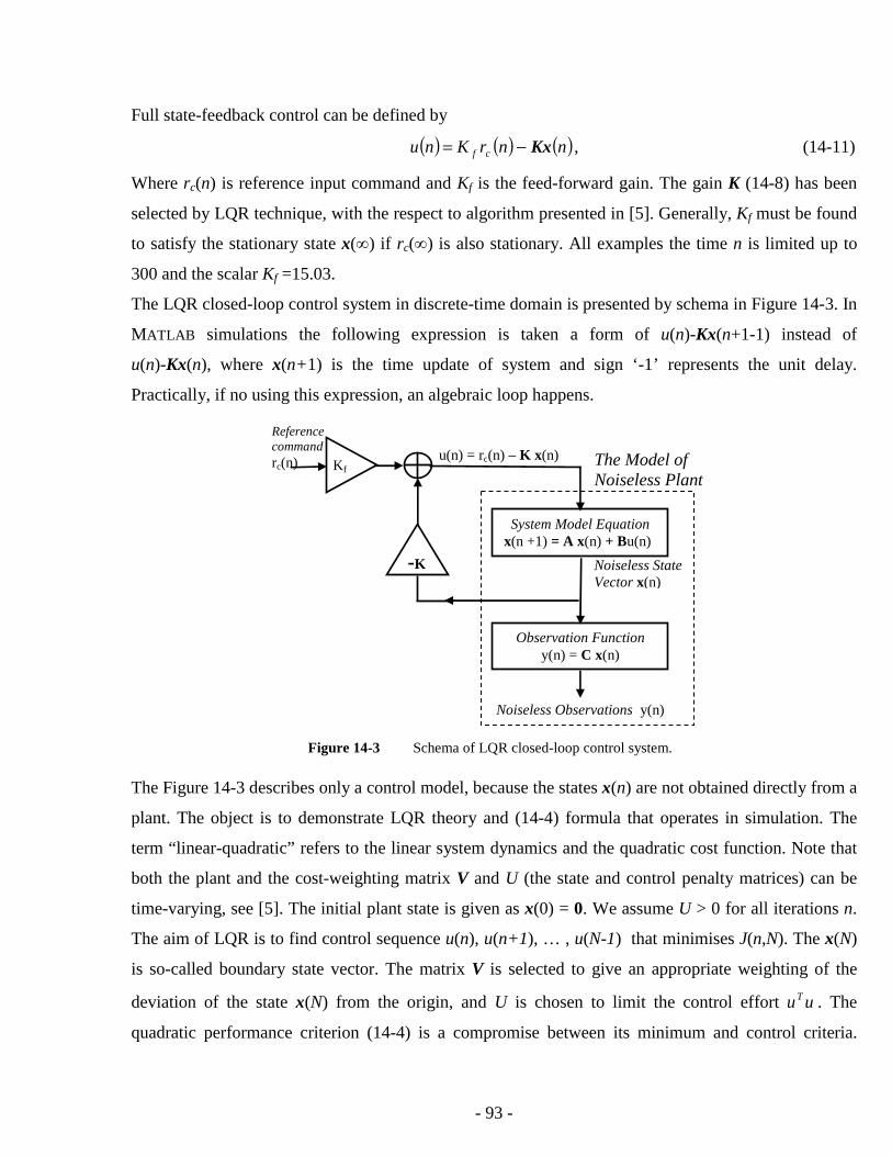
- 93 -

Full state-feedback control can be defined by

( ) ( ) ( )nnrKnu cf Kx−= , (14-11)

Where rc(n) is reference input command and Kf is the feed-forward gain. The gain K (14-8) has been

selected by LQR technique, with the respect to algorithm presented in [5]. Generally, Kf must be found

to satisfy the stationary state x(∞) if rc(∞) is also stationary. All examples the time n is limited up to

300 and the scalar Kf =15.03.

The LQR closed-loop control system in discrete-time domain is presented by schema in Figure 14-3. In

MATLAB simulations the following expression is taken a form of u(n)-Kx(n+1-1) instead of

u(n)-Kx(n), where x(n+1) is the time update of system and sign ‘-1’ represents the unit delay.

Practically, if no using this expression, an algebraic loop happens.

The Figure 14-3 describes only a control model, because the states x(n) are not obtained directly from a

plant. The object is to demonstrate LQR theory and (14-4) formula that operates in simulation. The

term “linear-quadratic” refers to the linear system dynamics and the quadratic cost function. Note that

both the plant and the cost-weighting matrix V and U (the state and control penalty matrices) can be

time-varying, see [5]. The initial plant state is given as x(0) = 0. We assume U > 0 for all iterations n.

The aim of LQR is to find control sequence u(n), u(n+1), … , u(N-1) that minimises J(n,N). The x(N)

is so-called boundary state vector. The matrix V is selected to give an appropriate weighting of the

deviation of the state x(N) from the origin, and U is chosen to limit the control effort uuT . The

quadratic performance criterion (14-4) is a compromise between its minimum and control criteria.

Reference command rc(n) The Model of

Noiseless Plant

Noiseless State Vector x(n)

Noiseless Observations y(n)

System Model Equation x(n +1) = A x(n) + Bu(n)

Observation Function y(n) = C x(n)

-K

u(n) = rc(n) – K x(n)

Figure 14-3 Schema of LQR closed-loop control system.

Kf

- 94 -

Only defaulted V to U ratio is important and if another ratio is larger than the defaulted one, then

deviations of x(n) from x(N) will be penalised heavily relative to deviations of u(n) from u(N). On the

other hand, if the control energy been small is important, then we should select a lover ratio than the

defaulted one, and the state will not quickly converge to x(N). In our case, the V to U ratio matters for

finding the LQR closed-loop (state-feedback) gain K. After many performed iterations of S and

consequent K computation satisfied the control criteria. The blue or red curve depicts ( ) ( )n,nyv1 1x≡

response of plant with or without LQR, respectively in Figure 14-4. The curve of rc(n) reference input

command is shown in green. This plant’s time behaviour x(1,n) is caused by u(n) shown in

Figure 14-5. Expression ( ) ( )n,nyv1 1x≡ is valid in Unit 14 to 14.1.

Both Figures 14-4 and 14-5 describe LQR control system performance.

50 100 150 200 250 3000

0.5

1

1.5

2

2.5

3

3.5Step Responses of Plant (the 10th order filter)

Discrete Time [n]

Ste

p R

espo

nses

Plant Response of Closed-Loop; Kf=15.03 K=[1x10]

Pure Response of Plant; Kf=1, K=0

Control Signal

Figure 14-4 Step responses of system with/without LQR, rc(n) in green.

Reference input command

- 95 -

When using third order filter as system model dynamics, stationary diagonal matrix should be selected

V been equal to 0.098I and U = 1 to fully satisfy control criteria mentioned on page 90. The system

dynamics and appropriate noises are clarified especially for LQR control system on page 89.

The sequence of LQR closed-loop control gain K is obtained by using (14-5) and (14-7).

980 982 984 986 988 990 992 994 996 998 1000

-1400

-1200

-1000

-800

-600

-400

-200

0

200

400Sequence of LQR Gain in Closed Loop of the 3rd Order Filter

K v

ecto

r se

quen

ce

Backward Iterations [i]

K(1,n)

K(2,n)

K(3,n)

Figure 14-6 Sequence of LQR closed-loop control gain for third order filter.

50 100 150 200 250 300 -5

0

5

10

15

20

25

30

35

Discrete Time [n]

Plant Input; Kf = 15.03, K = [1x10] vector

Figure 14-5 Input of plant in closed-LQR-loop (the 10th order filter).

- 96 -

50 100 150 200 250 300 -5

0

5

10

15

20

25

Discrete Time [n]

Plant Input in LQR loop

Figure 14-8 Input of plant in closed LQR loop (the 3rd order filter).

The gain K is found as

[ ]3.74 3.789 3.8 . (14-12)

Feed-forward gain Kf = 10.206. Following the schema in Figure 14-3, noiseless observations response

of plant is depict in Figure 14-7. Observations signal yv1(n) of system with LQR satisfies the control

criteria in which the overshoot is less than 5% and the form of steep response has been achieved. The

input control signal of plant is depict in Figure 14-8.

0 50 100 150 200 250 3000

0.5

1

1.5

2

2.5

3

3.5Step Responses of Plant (the 3rd order filter)

Discrete Time [n]

Ste

p R

espo

nse

of P

lant

Response of Plant in Closed LQR Loop; Kp = 10.206

Response of Plant in Open LQR Loop; Kp = 1, K = 0

Control Signal u(n)Reference input command

Figure 14-7 Step responses of system with/without LQR, rc(n) in green.

- 97 -

The third condition of control objectives is satisfying quite badly as shown in Figure 14-9.

The LQR gain (14-11) must be additionally multiplied by 49 to make the control conditions completely

satisfied. To fulfil the first condition, high frequency band is dominated and flat excepting zero in

transfer function at normalised frequency 0.1. In contrast, the blue curve hyper-belongs to pure

simulation of plan/system without any LQR.

0 0.1 0.2 0.3 0.4 0.5 0.6 0.7 0.8 0.9 1-200

-150

-100

-50

0

50


Pha

se (

degr

ees)

0 0.1 0.2 0.3 0.4 0.5 0.6 0.7 0.8 0.9 1-40

-30

-20

-10

0

10


Mag

nitu

de (

dB)

Frequency and Phase Response of Plant ( the 3rd order filter )

Plant in Closed LQR Loop; u=Kronecker -49K x(n/n),Kp = 10.206

Plant in Open LQR Loop; u=Kronecker, Kp = 1

Plant in Closed LQR Loop; u=Kronecker -49K x(n/n),Kp = 10.206

Plant in Open LQR Loop; u=Kronecker, Kp = 1

Figure 14-9 Frequency and phase response of LQR closed-loop system with third order filter.

- 98 -

14.1 Examples in Linear Quadratic Regulator using a nonlinear actuator

An exercise presents the focus on how to overcome undesirable negative range coming to an

actuator in modified LQR. The actuator provides positive output as u(n) assumed to be e.g. a heat in air

conditioning system without cooling (negative range – outcoming energy). As one can see in Figure

14-5, the control input u(n) of plant comes into negative range. If this range is saturated to zero by an

actuator, the gain K (14-8) based on LQR close-loop produces high overshoots. To ensure LQR

operating in linear (positive) range of u(t), the control system must behave in linear filtering. Hence we

like to find a new LQR closed-loop gain to solve mentioned problem with reference input command

rc(n) given by (14-3). Of course this example deals with new time behaviour of rc(n) and LQR gain:

[ ]113.3- 203.4- 322.9- 465.9- 612.9- 720.4- 708.1- 440.5- 298.4 1836 , (14-13)

where feed-forward gain Kf = 7.21 approximately. The LQR closed-loop gain K has been found due to

selected stationary diagonal matrix V is equal to 8.81x10-3 I and U = 1 to satisfy control objectives :

1. Steep response such as a short propagation time,

2. Minimum overshoot been less than 5 % of the stable value,

3. Least flat or descending frequency response,

4. Undesirable negative excitation in u(n) has to be overcome by (14-13) in modified LQR control

system.

The new concept introduced to (14-13) shows the yv1(n) that is a response in modified LQR with

nonlinear actuator, see red curve in Figure 14.1-1. The typical response shown in dashed curve is

provided with fully linear LQR control system, where the rc(n) has not limited range with appropriate

K, see the expression (14-8) and Figure 14-4. These two responses differ. The controlled system with

nonlinear actuator gives a bit slower response than the controlled system with full actuator’s range,

although the control criteria are satisfied. The input control signal u(n) is presented in Figure 14.1-2.

There one can see that the blue curve never crosses the unwanted negative range. Thus the linear

filtering is ensured in this case on actuator’s nonlinearity, and input control signal does not reach

negative values.

- 99 -

A fuzzy gain scheduler might be needed due to a nonlinear actuator, if rc(n) is not restricted to (14-3).

50 100 150 200 250 3000

2

4

6

8

10

12

14

16

18Input of Plant in Closed-LQR-Loop (the 10th order filter)

Discrete Time [n]

The

Ste

p R

espo

nse

of P

lant

Inp

ut u

(n)

Plant Input in Closed-LQR-Loop with Limitted Input Range

Figure 14.1-2 Input of plant in closed LQR loop (new gain, the 10th order filter).

50 100 150 200 250 3000

0.5

1

1.5

2

2.5

3

3.5Plant Responses (the 10th order filter)

Discrete Time [n]

Ste

p R

espo

nse

of P

lant

and

KF

Plant Response in case of Unlimitted Range

in Limitted Range,Closed-LQR-Loop;Kf=7.2098,K=[1x10]Pure Response of Plant in Open LQR Loop; Kf=1, K=0

Control Signal u(n)

Figure 14.1-1 Step responses of system with/without LQR, rc(n) and new response.

Reference input command

- 100 -

14.2 Examples in Linear Quadratic Gaussian design

This section focuses on some exercises of proposed regulator in linear-quadratic Gaussian, LQG,

design. Two stochastic discrete-time systems will be implemented in LQG and tested separately. The

first system follows the behaviour of tenth order filter to be called a system of tenth order, which:

• system model equation is given by (13-4) and

• observations (sensor) model equation is given by (13-5), where considered A, B and C matrices

are given by (13-1) to (13-3), respectively.

The second system of third order can be described by:

• system model equation is given by (12-1), and

• observation model equation is given by (12-2).

Observation and sensor noises are now fully employed. The Unit 6 deals with those noises models to

be used here. The process noise and sensor noises are uncorrelated and their variances are specified in

Unit 6. The w(n) noise is only one stream used the same in all simulations. Reference input command

rc(n) is given by (14-3). We have to note that the expression ( ) ( ) ( )nvnny 11v1 += xC due to stochastic

systems mentioned above been valid up to Section 14.3. This expression provides a model of first

observation of a plant, where ( )nyv1 and ( )nx will be investigated.

In complicate modern systems may be no priori guidelines for selecting the compensator structure. In

this case, a combination of linear-quadratic state-feedback regulator and state estimator proves very

usefulness. This combination is known as linear-quadratic Gaussian design, and its structure is shown

in Figure 14.2-1. There, the LQR problem and Kalman filter can be coupled together to design LQG.

In mathematics, this procedure is called linear-quadratic Gaussian problem. An important advantage of

LQG design is that the compensator structure is given by procedure that needs not be known

beforehand. This makes LQG design useful in the control of e.g., aircraft engines, helicopters, space

structures and robotics, where an appropriate compensator structure may be not known. By referring to

Figure 14.2-1, the LQR’s state-feedback gain K was selected by LQR technique in Unit 14. The

Kalman filter and its innovation KF gain M(n) was found in either Unit 2 – 5 or 6. Both gains were

designed separately to yield closed-loop plant behaviour and observer behaviour. This is the separation

- 101 -

Kf rc(n) - K x(n|n) = u(n)

Kf

-K

Actuator H(p) = 1

u(t)

KF

u(n)

yv(n)

Reference command rc(n)

LQG of CLOSED-LOOP in Discrete Time Domain

x(n|n)

DAC

Stochastic State-Space Model in Continuous Time Domain

Process Noise w(t)

u(t) + w(t)

Noisy State Vector x(t)

Noisy Observations yv(n)

Stochastic System Model Equation

w(t)] [u(t) (t) (t) ++= Γx Fx.

Equation of Stochastic Observations yv(t) = C x(t) + v(t)

ADC

Figure 14.2-1 Closed-loop schema in LQG design.

principle which is at the heart of modern controls design. Two important notifications of the separation

principle are made when close-loop stability is guaranteed and good software is available. The first

main idea of structure in Figure 14.2-1 is to perform plant control, second that the KF should estimate

plant states optimally. The LQG described briefly above can be running on a digital signal processor,

consequently that is the reason of shown LQG part in discrete-time domain and plant naturally in

continuous-time domain.

To evaluate the states in plant from the above structure of LQG, we need to specify the mean square

error – MSE and root mean square error – RMSE as follows:

( ) ( ) ( ) ( ) ∫∫ =⎟⎠⎞

⎜⎝⎛ −⎟

⎠⎞

⎜⎝⎛ −= xdtxdtttttMSE T

t

Loop-ClosedLoop-ClosedT

Loop-ClosedLoop-Closed300

0300

1 ~~xxxx , (14-14)

MSERMSE = , (14-15)

where the denominator simplifies the expression for power of states ( ) Loop-Closedtx . This states vector is

loaded from plant in LQG closed control loop with KF and exactly known Q and R. To employ AKF in

LQG, the tilde is marked in (14-14). Additionally we focus on a performance of open-loop so-called

feed-forward control structure shown in Figure 14.2-2.

- 102 -

The gin K was found as:

1. system of tenth order, where corresponded control gain is given by (14-8);

2. system of third order, where corresponded vector (14-11) times 49.

Further statement considers Figures 14.2-3 and 14.2-4. Every simulation provides some results of:

a) LQR that controls the noiseless plant to be deterministic, with zero process and sensor

noise; see green curve in figures; the plant provides ( ) PlantNoiseLesstx and ( ) PlantNoiseLessv1 ty ,

b) stochastic plant controlled by open-loop LQR; see red curve in figures; here the plant

provides ( ) Loop-Opentx and ( ) Loop-Openv1 ty ,

c) stochastic plant controlled by closed-loop LQG regulator, where KF with exactly known

Q(n) and R(n); see blue curve in figures,

d) stochastic plant controlled by closed-loop LQG regulator, where adaptive fuzzy Kalman

filter (see Unit 13) is utilised; see black curve in figures, here the plant provides

( ) Loop-Closedtx and ( ) Loop-Closedv1 ty .

Practically the benefit on LQG design is coupled with last d option. A result referred to option a is the

target being never achieved.

Figure 14.2-2 Open-loop schema in LQR design.

u(n)=Kf rc(n) - K x(n)

LQR OPEN-LOOP in Discrete Time Domain

B

Ref. comm. rc(n)

x(n)

-K

z-1 A

x(n+1)

Kf

Stochastic State-Space Model in Discrete Time Domain

Process Noise w(n)

u(n) + w(n)

Noisy State Vector x(n)

Noisy Observations yv(n)

Stochastic System Model Equation x(n+1) = A x(n) + B [u(n) + w(n)]

Equation of Stochastic Observations yv(n) = C x(n) + v(n)

- 103 -

Option of b refers to pure control with open-loop LQR. This kind of regulator is established because of

simulation and regulators comparison. There a stochastic system model with w(n) and vi(n) noises is

supposed, where i = 1, 2, …, 10 (or 3).

Last two options c and d refer to the stochastic systems have been discussed, but a state-closed-loop

LQG design is applied in control. System states should be numerically near.. Additionally, it is

expected that an uncertainty extracted from those states should be a little toward an uncertainty

produced by plants state in option b. This fact should happen due to numerically very strong LQR gain

K that meaning high values of that gain. Intuitively, this strong gain causes high feed-forward Kf gain.

This kind of attenuation can be measured only in simulations. Of course main idea of LQR and

LQG/LTR design is nothing but optimal control. The gain K attenuates process noise in states and this

capability is a by-product and can be obtained from measured state in plant and observations

respectively as follows:

( ) ( )( ) ( ) ( )( )( ) ( )( ) ( ) ( )( )∑

∑

=

=

−−

−−=

300

0i

Loop-OpenPlantNoiseLessTLoop-OpenPlantNoiseLess

300

0i

Loop-ClosedPlantNoiseLessTLoop-ClosedPlantNoiseLess

nxnxnxnx

nxnxnxnxNNRx (14-16)

( ) ( )( )( ) ( )( )∑

∑

=

=

−

−=

300

0i

2Loop-Openv1

PlantNoiseLessv1

300

0i

2Loop-Closedv1

PlantNoiseLessv1

nyny

nynyNNRy . (14-17)

An assessment of a performance of LQG design based regulator and tenth order filter.

This part deals with performance of LQG design based regulator, Figure 14.2-1. Some results of that

regulator will be compared to some results of open-loop regulator, Figure 14.2-2. In this section, LQG

regulator has two modifications, such as to be with adaptive fuzzy logic Kalman filter (as AKF, see

Table 5-1) and conventional Kalman filter CoKF which bases on exactly known covariance of process

and sensor noise. Both estimators provide very similar observations yv1(n). This first observation

describes relative position of ferry, robot or motor’s rotor, etc. The second modification can be of

course only simulated and is useful such as reference regulator solving linear-quadratic Gaussian and

loop-transfer recovery (LQG/LTR) problem, [5]. To be honest, the rc(n) is Hevisideon pulse Һ(n-100).

The green curves in below figures represent observations of open-loop regulator, see Figure 14.2-2, but

without any noise. The same is illustrated in red with process and sensor noises in plant.

- 104 -

Figure 14.2-4 Observations obtained from different regulators with low power of process noise in plant.

0 50 100 150 200 250 300

-0.4

-0.2

0

0.2

0.4

0.6

0.8

1

1.2

1.4

1.6

Continuous Time [t]

O B S E R V A T I O N S

Comparison of Noiseless and Noisy Observations in LQR Loop,Plant Observations Performed by KF and AKF in LQG Loop;

Yv(n) of NoiseLess Plant in Open Loop of LQR. Yv(n) of Noisy Plant in Open Loop of LQR. Yv(n) of Noisy Plant in Closed LQG Loop (Exact Q,R) Yv(n) of Noisy Plant in Closed LQG Loop (AKF)

Figure 14.2-3 Observations obtained from different regulators with high power of process noise in plant.

0 50 100 150 200 250 300

-0.4

-0.2

0

0.2

0.4

0.6

0.8

1

1.2

1.4

1.6

Continuous Time [t]


Comparison of Noiseless and Noisy Observations in LQR Loop, Plant Observations Performed by KF and AKF in LQG Loop;

Yv(n) of NoiseLess Plant in Open Loop of LQR. Yv(n) of Noisy Plant in Open Loop of LQR. Yv(n) of Noisy Plant in Closed LQG Loop (Exact Q,R)Yv(n) of Noisy Plant in Closed LQG Loop (AKF)

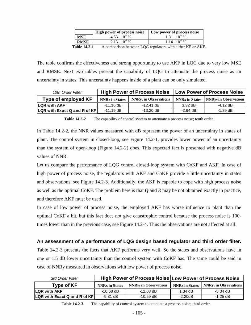
- 105 -

High power of process noise Low power of process noise MSE 4.53 . 10-4 % 1.31 . 10-4 % RMSE 2.13 . 10-1 % 1.14 . 10-1 %

Table 14.2-1 A comparison between LQG regulators with either KF or AKF.

The table confirms the effectiveness and strong opportunity to use AKF in LQG due to very low MSE

and RMSE. Next two tables present the capability of LQG to attenuate the process noise as an

uncertainty in states. This uncertainty happens inside of a plant can be only simulated.

In Table 14.2-2, the NNR values measured with dB represent the power of an uncertainty in states of

plant. The control system in closed-loop, see Figure 14.2-1, provides lower power of an uncertainty

than the system of open-loop (Figure 14.2-2) does. This expected fact is presented with negative dB

values of NNR.

Let us compare the performance of LQG control closed-loop system with CoKF and AKF. In case of

high power of process noise, the regulators with AKF and CoKF provide a little uncertainty in states

and observations, see Figure 14.2-3. Additionally, the AKF is capable to cope with high process noise

as well as the optimal CoKF. The problem here is that Q and R may be not obtained exactly in practice,

and therefore AKF must be used.

In case of low power of process noise, the employed AKF has worse influence to plant than the

optimal CoKF a bit, but this fact does not give catastrophic control because the process noise is 100-

times lower than in the previous case, see Figure 14.2-4. Thus the observations are not affected at all.

An assessment of a performance of LQG design based regulator and third order filter.

Table 14.2-3 presents the facts that AKF performs very well. So the states and observations have in

one or 1.5 dB lower uncertainty than the control system with CoKF has. The same could be said in

case of NNRy measured in observations with low power of process noise.

Table 14.2-2 The capability of control system to attenuate a process noise; tenth order.

10th Order Filter High Power of Process Noise Low Power of Process NoiseType of employed KF NNRx in States NNRyv in Observations NNRx in States NNRyv in Observations

LQR with AKF -11.16 dB -12.41 dB 3.32 dB -4.12 dBLQR with Exact Q and R of KF -11.19 dB -13.20 dB -2.64 dB -1.39 dB

Table 14.2-3 The capability of control system to attenuate a process noise; third order.

3rd Order Filter High Power of Process Noise Low Power of Process NoiseType of KF NNRx in States NNRyv in Observations NNRx in States NNRyv in Observations

LQR with AKF -10.68 dB -12.08 dB 1.34 dB -5.34 dBLQR with Exact Q and R of KF -9.31 dB -10.59 dB -2.20dB -1.25 dB

- 106 -

14.3 An example of multi-state-sensor control system in LQG design

Previous section solved the control problem of a system composed of one sensor. This section

deals with LQG based regulator and three sensors employed in the control. Here the LQR gain is taken

over the Section 14.2. Additionally, we assume adaptive decentralized Kalman filter-ADKF in multi-

state multi-sensor fusion. To specify the control strategy, decentralized structure should be introduced.

Our example contains three nodes and every node contains one processor executing program. Thus

every node is sensing independent observations yvi(n), where i = 1, 2, 3. The model contains three

nodes as well as usually three components are controlled such as position, velocity and acceleration.

The term “multi-state fusion” has been deduced. By the way, every processor should perform Kalman

filtering needed for estimation in LQG problem, and linear-quadratic control in digital-time domain.

All provide the same state estimation The Figure 14.3-1 depicts observations produced by regulators.

Figure 14.3-1 Observations obtained from different LQG controllers with high power of process noise in plant.

0 50 100 150 200 250 300

-0.4

-0.2

0

0.2

0.4

0.6

0.8

1

1.2

1.4

1.6

Continuous Time [t]

O B S E R V A T I O N S Yv(n) of NoiseLess Plant in Open Loop of LQR

Yv(n) of Noisy Plant in Open Loop of LQRYv(n) of Noisy Plant in Closed LQG Loop (Exact Q,R) Yv(n) of Noisy Plant in Closed LQG Loop (ADKF)

Plant Observations Performed by DKF and ADKF in LQG Loop;

- 107 -

Figure 14.3-3 presents the schema of LQG problem based control with ADKF, but as an alternative the

DKF can be used instead. The nodes share their VEIi(n) and SEIi(n) information to update their state

estimates, where i = 1, 2 and 3. This is SIMO model.

We would like to compare some results of LQG (Table 14.3-1) with three sensors and ADKF toward

the LQG (Table 14.2-3) with one sensor and AKF described in Section 14.2. In case of high power of

process noise, both regulators provide comparable noisy states of plant and observation yv1(n). In case

of low power, our regulator (Table 14.3-1) with three sensors performs in 2.81 dB noiseless controlled

state of plant than regulator (Table 14.2-3) with one sensor. The system model equation (12-1) remains

been used here too.

Table 14.3-1 The capability of complicate control system to attenuate a process noise.

3rd Order Filter High Power of Process Noise Low Power of Process NoiseLQG Closed Loop NNRx in States NNRyv in Observations NNRx in States NNRyv in Observations

LQR with ADKF -10.35 dB -10.99 dB -1.47 dB -2.88 dB

Figure 14.3-2 Observations obtained from different LQG controllers with low power of process noise in plant.

0 50 100 150 200 250 300

-0.4

-0.2

0

0.2

0.4

0.6

0.8

1

1.2

1.4

1.6

Continuous Time [t]


Plant Observations Performed by DKF and ADKF in LQG Loop;

Yv(n) of NoiseLess Plant in Open Loop of LQR Yv(n) of Noisy Plant in Open Loop Yv(n) of Noisy Plant in Closed LQG Loop (Exact Q,R)Yv(n) of Noisy Plant in Closed LQG Loop (ADKF)

- 108 -

Figure 14.3-3 Schema of LQG problem based control in multi-sensor multi-state system.

Stochastic State-Space Model in Continuous Time Domain

Process Noise w(t)

u(t) + w(t)

Noisy State Vector x(t)

Stochastic System Model Equation

)]Γx Fx.

w(t [u(t) (t) (t) ++=

Noisy Observations yv1(n) in Discrete Time Domain

DAC

Equation of Stochastic Observations ( Sensor 1 )

yv1(t) = [1 0 0]x(t) + v1(t)

u(n) = Kf rc(n) – K x(n|n)

ADKF 1

-K

Kf



DAC


yv2(t) = [0 1 0]x(t) + v2(t)

u(n) = Kf rc(n) – K x(n|n)

ADKF 2

-K

Kf



DAC


yv3(t) = [0 0 1]x(t) + v3(t) u(n) = Kf rc(n) – K x(n|n)

ADKF 3

-K

Kf


SEI 1, VEI 1

and SEI 3, VEI 3

SEI 2, VEI 2 and

SEI 3, VEI 3

SEI 1, VEI1 and

SEI 2, VEI 2

The Data Interconnection

Actuator H(p) = 1

DAC

Embedded LQR and ADKF in Sensor



x(n|n) x(n|n)

x(n|n)

- 109 -

14.4 Conclusions

Below we apply the last question asked in section 1.1 to this conclusion:

“Demonstrate a functionality of an optimal regulator in Linear Quadratic Gaussian, LQG, problem, so

that a single/multi dimensional output of a linear system takes control in backward closed loop. In

addition to linear system, the (adaptive) Kalman filter should be investigated.”

The Unit 14 demonstrates technique of LQR closed-loop problem as an approach to simple exercises.

This technique controls the step response of system to satisfy control criteria.

Section 14.1 deals with similar exercises with considered nonlinear actuator. The advantage of this

control solution is knowledge on actuator. A different performance occurs between LQR presented in

last two sections.

In sections 14.2 and 14.3 the system controlled in closed-loop provides lower uncertainty than in open-

loop control. All measurements are performed in states and observations and AKF is employed in

LQG. Section 14.3 deals with LQG problem based regulator and three sensors fully employed in the

control. There the adaptive decentralized Kalman filter-ADKF is employed in multi-sensor multi-state

fusion additionally. The states provided to LQG + ADKF is nearly same with in LQG + DKF.

Considered compensator has very high order equal to the order of plant. This means that it has too

many parameters to be conveniently gain scheduled. It might be possible to use reduced-order

compensator principle component analysis-PCA as one of many other techniques.

- 110 -

15 MAIN SUMMARY AND CONCLUSIONS

This manuscript is composed of two main parts as well as Kalman-Filter techniques, MATLAB

simulations and tests.

The first part employs Kalman-Filter technique with one sensor, centralized and decentralized Kalman-

Filter technique and technique of adaptive Kalman-Filter. Unit 2 to 5 are related to those techniques.

The second part deals with some experiments of conventional Kalman-Filter with one sensor so-called

CoKF; centralized Kalman-Filter with many sensors so-called CKF; decentralized-centralized Kalman-

Filter comparison – DKF. Then the followings are associated with experiments in problematic of bias,

broken node, drift effect on state estimation in DKF, algorithm of fault detection and isolation in

sensors, algorithm and exercising on adaptive fuzzy logic decentralized Kalman-Filter, LQR and LQG.

The section 1.1 gives seven questions to be answered one by one below.

We apply the first question to summary:

“Demonstrate state estimation identity of decentralized Kalman filter, DKF, and centralized Kalman

filter, CKF, in an experimental simulation study assuming uniform filter conditions. What are

differences?”

The states dealt with both estimators appear nearly identical. This summary refers to Unit 8.

We apply the second question to summary:

“Measure a mean square error, MSE, of state estimation in simulated DKF model that contains a sensor

been affected by a bias with uniform filter conditions. Simulations have to be performed with total

numbers of sensors such as two and five. How does the MSE depend on the total number of sensors?

Tests need to be performed, namely with:

constant bias,

linearly increased bias.”

- 111 -

The relation between mean square error and the total number of sensors appeared been valid same for

both bias types. This relation is explained by two and five sensors, where MSE / MSE 5DKF2DKF is

equal to number of sensors ratio given by 2

5. The MSE2DKF is the mean square error of state estimation

in DKF model composed by two sensors, etc. This summary refers to Unit 9.

We apply the third question to summary:

“Measure the MSE of state estimation in simulated DKF model that contains a broken sensor with

uniform filter conditions. Simulations have to be performed with two and five total numbers of sensors.

How does the MSE depend on the total number of sensors?”

The DKF model is composed of two and five sensors, where only one of them is broken.

Ratio MSE / MSE 5DKF2DKF is equal to 2.496 and 2.501 assuming high and low power of process

noise, respectively. Both values (2.496 and 2.501) are numerically near the expected value 2.5. The

MSE2DKF is the mean square error of state estimation in DKF model composed by two sensors, etc.

This summary refers to Unit 10.

We apply the fourth question to summary:

“Measure the MSE of state estimation in DKF model that contains a sensor affected by a drift with

uniform filter conditions. Simulations have to be performed by using one, two, and five total numbers

of sensors. How does the MSE depend on the total number of sensors?”

As an approximation, the MSE is linearly proportional to the used total number of sensors. For

example in our case of 2 sensors model, the estimator gives four times lower MSE of state estimation

than DKF with one sensor. Five sensors DKF performs with 25-times lower MSE than one sensor

DKF. Exponential drift is assumed. This summary refers to Unit 11.

- 112 -

We apply the fifth question to summary:

“Find out a fault detection and isolation, FDI, algorithm been possibly useable for DKF model. This

model has to be tested with a minor number of affected sensors by exponentially descending drifts.

What is a performance of this DKF model with applied FDI algorithm, when:

one sensor is affected by the drift, and additionally two sensors are correct;

two sensors are affected by two miscellaneous drifts, plus one correct sensor?”

The major requirement on FDI algorithm is the availability to multiple observations. It was shown on

how to apply FDI algorithm to the problem of DKF model with faults in sensors. The FDI algorithm

was already found out. Firstly the question related to one affected sensor is to be answered below.

Our simulation results shown that the DKF model with FDI algorithm yields 75% reliability of

FDI performance insomuch that a pure DKF model without FDI provides exactly 0% reliability. The

FDI reliability is not meant to be state estimation accuracy, although its relative MSE is about 0.01. In

case of high process noise, the simulation results gave about 70% reliability of FDI algorithm. The 5

percentage aggravation is caused by 100-times higher power of process noise, where cross-correlation

function used in FDI system is disturbed by that.

Having two affected sensors by exponential drifts, the FDI reliability was 84%. By considered

100-times higher power of process noise, the reliability was reduced down to 54%, but relative MSE of

state estimation was about 0.11. This is the FDI imperfection with major number of corrupted sensors.

The DKF models use multi-state, multi-sensor system, meaning fusion with different observations

quality. Time behaviour of u(n) is sinus as a still oscillated signal rather used than a less problematic

step pulse. This summary refers to Unit 12.

We apply the sixth question to summary:

“Test an algorithm of adaptive Kalman filter, AKF, supported by fuzzy logic to meet the Kalman filter

functionality, by definition of an optimal state estimation in Kalman filtering, with a strategy of an

adapted process noise covariance Q matrix and observation R1 noise variance. Suppose both prior Q

and R1 are unknown. The reasonable effort should be made to additionally estimate the covariance

- 113 -

matrices when the noise streams are unknown. So that, the AKF extends KF functionality to meet the

practical needs when changing from traditional KF.”

To exam the AKF with high power of process noise, a bit better state estimation accuracy occasionally

occurs than the conventional Kalman filter provides. Considering lower power of process noise than

the power of sensor noise, the w(n) and v1(n) are very little and can not worse the state estimation at all,

especially in control. The adaptive algorithm is considerable, otherwise an absence of that

inappropriate Q and R1 setting may cause a practical divergence of estimator, but this effect has been

never found in AKF. This summary refers to Unit 13.

We apply the seventh question to summary:

“Demonstrate a functionality of an optimal regulator in Linear Quadratic Gaussian, LQG, problem, so

that a single/multi dimensional output of a linear system takes control in backward closed loop. In

addition to linear system, the (adaptive) Kalman filter should be investigated.”

The technique of LQR in closed-loop controls the step response of system to satisfy control criteria.

Section 14.1 deals with some exercises with nonlinear actuator. A slight performance occurs between

LQR with linear/nonlinear actuator. Of course it is depending on the type of nonlinearity to be

presented in specific control.

The LQG has a capability to attenuate system’s uncertainty in controlled LQG closed-loop. This is of

course a by-product. The main product is good states in plant that can be based on comparison of LQG

and LQR.

In addition to ADKF employed in multi-sensor multi-state fusion, the states provided to LQG + ADKF

is nearly same with in LQG + DKF. This summary refers to Unit 14.

- 114 -

REFERENCES

[1] GOODWIN Clifford G., and SIN K. S. (1984). “Adaptive Filtering Prediction and Control,”

PRENTICE-HALL, INC., Englewood Cliffs, New Jersey 07632.

[2] FRIEDLAND B. (1996). “Advanced Control System Design,” PRENTICE-HALL, INC., A

Simon & Schuster Company Englewood Cliffs, New Jersey 07632

[3] GELB A., KASPER J. F., NASH R. A., PRICE C. F., and SUTHERLAND A. A., (1999).

“Applied Optimal Estimation,” Massachusetts Institute of Technology Cambridge,

Massachusetts, and London, England, Library of Congress Catalog Card Number:

741604.

[4] MOHINDER S. GREWAL, and ANGUS P. ANDREWS, (1993). “KALMAN FILTERING

Theory and Practice,” PRENTICE-HALL, INC., A Simon & Schuster Company

Englewood Cliffs, New Jersey 07632.

[5] FRANK L. LEWIS, and VASSILIS L. SYRMOS, (1993). “OPTIMAL CONTROL,” A Wiley-

Interscience Publication, A John Wiley & Sons Inc., New York, Chichester, Brisbane,

Toronto, Singapore.

[6] ISERMANN R. (Rolf), (2003). “Mechatronic Systems : fundamentals,” 1.Mechatronics and

2.Microelectromechanical systems, British Library Cataloguing in Publication Data.

[7] MATLAB Release 12 Help.

[8] VERHAEGEN M. H., (March 1989). “Improved understanding of the loss-of-symmetry

phenomenon in the conventional Kalman filter,” Automatic Control, IEEE Transactions,

Vol.34, Iss.3, pp. 331-333.

- 115 -

[9] RAO B. S., and DURRANT-WHYTE H. F., (September 1991). “Fully decentralized

algorithm for multisensor Kalman filtering,” IEE PROCEEDINGS-D, Vol. 138, No. 5, pp.

413-420.

http://portal.acm.org/citation.cfm?id=942356&dl=ACM&coll=portal

[10] PAO L. Y., and BALTZ N. T. (June 1999). “Control of Sensor Information in Distributed

Multisensor Systems,” Proc. American Control Conference, San Diego, CA,pp. 2397-2401.

[11] DURRANT-WHYTE H. F., and LEONARD J. J., (13-18 May 1990). “Toward a fully

decentralized architecture for multi-sensor data fusion,” Robotics and Automation,

1990.Proceedings., IEEE International Conference, Vol.2, pp. 1331 – 1336.

http://ieeexplore.ieee.org/iel5/484/3534/00126185.pdf?tp=&arnumber=126185&isnumber=3534

[12] DURRANT-WHYTE H. F., RAO B. Y. S., and HU H., (4 Feb 1991). “Toward a fully

decentralized architecture for multi-sensor data fusion,” Principles and Applications of

Data Fusion, IEE Colloquium, pp.2/1 - 2/4.


[13] DURRANT-WHYTE H. F., (19 Feb 1991). “Elements of sensor fusion,” Intelligent Control,

IEE Colloquium, pp.5/1 - 5/2.


[14] DAILEY DANIEL J., HARN PATRICIA, and LIN PO - JUNG, (April 1996). “ITS Data Fusion,”

Final Research Report T9903, University of Washington Seattle, Washington State

Department of Transportation Technical Monitor.

http://www.its.washington.edu/pubs/fusion_report.pdf

[15] WEI M., and SCHWARTZ K. P., (20-23 March 1990). “Testing a decentralized filter for

GPS/INS integration,” Position Location and Navigation Symposium, 1990. Record. 'The

1990's - A Decade of Excellence in the Navigation Sciences'. IEEE PLANS '90., IEEE , pp.

429 – 435.


- 116 -

[16] STROBEL N., SPORS S. and RABENSTEIN R., (5-9 June 2000). “Joint audio-video object

localization using a recursive multi-state multi-sensor estimator,” Acoustics, Speech, and

Signal Processing, 2000. ICASSP '00. Proceedings. 2000 IEEE International

Conference, Vol.6, pp.2397 - 2400 vol.4.


[17] TAE-GYOO LEE., (December 2003). “Centralized Kalman Filter with Adaptive

Measurement Fusion: its Application to a GPS/SDINS Integration System with an

Additional Sensor,” International Journal of Control, Automation, and Systems Vol. 1,

No. 4.

[18] LOEBIS D., CHUDLEY J., and SUTTON R. (1 Aprile 2004). “A fuzzy Kalman filter optimized

using a multi-objective genetic algorithm for enhanced autonomous underwater vehicle

navigation,” Proceedings of the I MECH E Part M Journal of Engineering for the

Maritime Envi, vol. 218, no. 1, pp. 53-69(17).

[19] RAY ASOK, and LUCK ROGELIO (Aprile 7-12 1991). “An Introduction to Sensor Signal

Validation in Redundant Measurement Systems,” The 1991 IEEE International

Conference on Robotics and Automation, Hyatt Regency in Sacramento, California, pp.

44-49.

[20] FITZGERALG R.J. (1997). “Divergence of the Kalman Filter,” IEEE Transaction on

Automatic Control, vol. AC-16, no. 6, pp.736-747.

[21] ROGÉRIO BASTOS QUIRINO and CELSO PASCOLI BOTTURA (January – April 2001). “An

approach for distributed Kalman filtering,” SBA Control and Automation, vol. 12, no. 01.

- 117 -

APPENDIX A

A A BRIEF REVIEW OF SOME RESULTS FROM CoKF TECHNIQUES

A.1 Model 3 of KF Result (referring to Unit 6)

A.2 Simulink Block of Model 1 of KF (referring to Table 2-1 in Chapter 2)

0 10 20 30 40 50 60 70 80 90 100-4

-3

-2

-1

0

1

2

3

4

Discrete Time [n]

Out

puts

Conventional Kalman filter response, MODEL 3 of CoKF

Cx(n) of Plantye(n) of Model 3 of CoKF

0 10 20 30 40 50 60 70 80 90 100-3

-2

-1

0

1

2

3

Discrete Time [n]

Err

ors

Error

Sensor Noise v(n)Cx(n) - ye(n)

- 118 -

- 119 -

A.3 Simulink Block of Model 2 of KF (referring to Table 2-2 in Unit 2)

- 120 -

A.4 Simulink Block of Model 3 of KF (referring to Table 2-3 in Unit 2)

- 121 -

A.5 Improvement of CoKF in Simulink MATLAB Program (referring to the flowchart of Figure 2.1-1)

- 122 -

APPENDIX B

B A BRIEF REVIEW OF SOME RESULTS FROM CKF TECHNIQUES

B.1 Inner Block Connection of Fully Centralized KF - Model 3 of CKF (referring to Table 3-3 in Unit 3)

- 123 -

B.2 Improvement of Model 3 of CKF in Simulink MATLAB Program (referring to the treated equation (3-21) in flowchart of Figure 3.1-1, Unit 3)

- 124 -

APPENDIX C

C A BRIEF REVIEW OF SOME TESTS AND MODELS

C.1 Two Nodes DKF model (referring to the tests in Unit 8)

- 125 -

C.2 Test of One Node CoKF model (referring to the Unit 11.1)

- 126 -

C.3 Test of Two Nodes DKF model (referring to the Units 9.1, 9.3, 10.1, and 11.2)

- 127 -

C.4 Test of Five Nodes DKF model (referring to the Units 9.2, 9.4, 10.2, and 11.3)

- 128 -

C.5 First Node Block Connection of DKF with FDI shown in Simulink MATLAB Program

kalman filtering in multi-sensor fusion - sme · kalman filtering in multi-sensor fusion tibor...

Documents