kalman filter applications - cornell university · kalman filter applications the kalman ﬁlter...

.

. Subject MI63: Kalman Filter Tank Filling

Kalman Filter Applications

The Kalman filter (see Subject MI37) is a very powerful toolwhen it comes to controlling noisy systems. The basic idea of aKalman filter is: Noisy data in⇒ hopefully less noisy data out.

The applications of a Kalman filter are numerous:

• Tracking objects (e.g., missiles, faces, heads, hands)

• Fitting Bezier patches to (noisy, moving, ...) point data

• Economics

• Navigation

• Many computer vision applications

– Stabilizing depth measurements

– Feature tracking

– Cluster tracking

– Fusing data from radar, laser scanner andstereo-cameras for depth and velocity measurements

– Many more

This lecture will help you understand some direct applicationsof the Kalman filter using numerical examples.

The examples that will be outlined are:

1. Simple 1D example, tracking the level in a tank (this pdf)

2. Integrating disparity using known ego-motion (in MI64)

September 2008

.


Predict-Update Equations

First, recall the time discrete Kalman filter equations (see MI37)and the predict-update equations as below:

Predict:x̂t|t−1 = Ftx̂t−1|t−1 + Btut

Pt|t−1 = FtPt−1|t−1FTt + Qt

Update:x̂t|t = x̂t|t−1 + Kt

(yt −Htx̂t|t−1

)Kt = Pt|t−1HT

t

(HtPt|t−1HT

t + Rt

)−1

Pt|t = (I−KtHt)Pt|t−1

wherex̂ : Estimated state.

F : State transition matrix (i.e., transition between states).

u : Control variables.

B : Control matrix (i.e., mapping control to state variables).

P : State variance matrix (i.e., error of estimation).

Q : Process variance matrix (i.e., error due to process).

y : Measurement variables.

H : Measurement matrix (i.e., mapping measurements onto state).

K : Kalman gain.

R : Measurement variance matrix (i.e., error from measurements).

Subscripts are as follows: t|t current time period, t− 1|t− 1previous time period, and t|t− 1 are intermediate steps.

September 2008

.


Model Definition Process

The Kalman filter removes noise by assuming a pre-definedmodel of a system. Therefore, the Kalman filter model must bemeaningful. It should be defined as follows:

1. Understand the situation: Look at the problem. Break itdown to the mathematical basics. If you don’t do this, youmay end up doing unneeded work.

2. Model the state process: Start with a basic model. It maynot work effectively at first, but this can be refined later.

3. Model the measurement process: Analyze how you aregoing to measure the process. The measurement space maynot be in the same space as the state (e.g., using an electricaldiode to measure weight, an electrical reading does noteasily translate to a weight).

4. Model the noise: This needs to be done for both the stateand measurement process. The base Kalman filter assumesGaussian (white) noise, so make the variance andcovariance (error) meaningful (i.e., make sure that the erroryou model is suitable for the situation).

5. Test the filter: Often overlooked, use synthetic data ifnecessary (e.g., if the process is not safe to test on a liveenvironment). See if the filter is behaving as it should.

6. Refine filter: Try to change the noise parameters (filter), asthis is the easiest to change. If necessary go back further,you may need to rethink the situation.

September 2008

.


Example: Water level in tank

1. Understanding the situation

We consider a simple situation showing a way to measure thelevel of water in a tank. This is shown in the figurea.

We are trying to estimate the level of water in the tank, which isunknown. The measurements obtained are from the level of the“float”. This could be an electronic device, or a simplemechanical device. The water could be:

• Filling, emptying or static (i.e., the average level of the tankis increasing, decreasing or not changing).• Sloshing or stagnant (i.e., the relative level of the float to the

average level of the tank is changing over time, or is static).

aTaken from http://www.cs.unc.edu/˜welch/kalman/kftool/

index.html

September 2008

.


First Option: A Static Model

2. Model the state process

We will outline several ways to model this simple situation,showing the power of a good Kalman filter model.

The first is the most basic model, the tank is level (i.e., the truelevel is constant L = c).

Using the equations from Page 2, the state variable can bereduced to a scalar (i.e., x̂ = x where x is the estimate of L).

We are assuming a constant model, therefore xt+1 = xt, soA = 0 and Ft = 1, for any t ≥ 0.

Control variables B and u are not used (i.e., both = 0).

3. Model the measurement process

In our model, we have the level of the float. This is representedby y = y.

The value we are measuring could be a scaled measurement(e.g., a 1 cm measurement on a mechanical dial could actuallybe about 10 cm in the “true” level of the tank). Think of yourpetrol gauge on your car, 1 cm can represent 10 L of petrol!

For simplicity, we will assume that the measurement is the exactsame scale as our state estimate x (i.e., H = 1).

September 2008

.


4. Model the noise

For this model, we are going to assume that there is noise fromthe measurement (i.e., R = r).

The process is a scalar, therefore P = p. And as the process isnot well defined, we will adjust the noise (i.e., Q = q).

We will now demonstrate the effects of changing these noiseparameters.

5. Test the filter

You can now see that you can simplify the equations from Page2. They simplify as follows:

Predict:

xt|t−1 = xt−1|t−1

pt|t−1 = pt−1|t−1 + qt

Update:

xt|t = xt|t−1 +Kt

(yt − xt|t−1

)Kt = pt|t−1

(pt|t−1 + r

)−1

pt|t = (1−Kt) pt|t−1

September 2008

.


The filter is now completely defined. Let’s put some numbersinto this model. For the first test, we assume the true level of thetank is L = 1.

We initialize the state with an arbitrary number, with anextremely high variance as it is completely unknown: x0 = 0and p0 = 1000. If you initialize with a more meaningfulvariable, you will get faster convergence. The system noise wewill choose will be q = 0.0001, as we think we have an accuratemodel. Let’s start this process.

Predict:

x1|0 = 0

p1|0 = 1000 + 0.0001

The hypothetical measurement we get is y1 = 0.9 (due to noise).We assume a measurement noise of r = 0.1.

Update:

K1 = 1000.0001(1000.0001 + 0.1)−1 = 0.9999

x1|1 = 0 + 0.9999 (0.9− 0) = 0.8999

p1|1 = (1− 0.9999) 1000.0001 = 0.1000

So you can see that Step 1, the initialization of 0, has beenbrought close to the true value of the system. Also, the variance(error) has been brought down to a reasonable value.

September 2008

.


Let’s do one more step:

Predict:

x2|1 = 0.8999

p2|1 = 0.1000 + 0.0001 = 0.1001

The hypothetical measurement we get this time is y2 = 0.8 (dueto noise).

Update:

K2 = 0.1001 (0.1001 + 0.1)−1 = 0.5002

x2|2 = 0.8999 + 0.5002 (0.8− 0.8999) = 0.8499

p2|2 = (1− 0.5002) 0.1001 = 0.0500

You can notice that the variance is reducing each time. If wecontinue (with hypothetical yt-values) this we get the followingresults:

Predict Update

t xt|t−1 pt|t−1 yt Kt xt|t pt|t

3 0.8499 0.0501 1.1 0.3339 0.9334 0.0334

4 0.9334 0.0335 1 0.2509 0.9501 0.0251

5 0.9501 0.0252 0.95 0.2012 0.9501 0.0201

6 0.9501 0.0202 1.05 0.1682 0.9669 0.0168

7 0.9669 0.0169 1.2 0.1447 1.0006 0.0145

8 1.0006 0.0146 0.9 0.1272 0.9878 0.0127

9 0.9878 0.0128 0.85 0.1136 0.9722 0.0114

10 0.9722 0.0115 1.15 0.1028 0.9905 0.0103

September 2008

.


Another reading sequence; try this:

Predict Update

t xt|t−1 pt|t−1 yt Kt xt|t pt|t

3 1.05

4 0.95

5 1.2

6 1.1

7 0.23

8 0.85

9 1.25

10 0.76

September 2008

.


You can see (Page 8) that the model successfully works. Afterstabilization (about t = 4) the estimated state is within 0.05 ofthe “true” value, even though the measurements are between0.8 and 1.2 (i.e., within 0.2 of the true value).

Over time we will get the following graph:

September 2008

.


So what have we established so far?

If we create a model based on the true situation, our estimatedstate will be close to the true value, even when themeasurements are very noisy (i.e., a 20% error, only produced a5% inaccuracy).

This is the main purpose of the Kalman filter.

But what happens if the true situation is different?

We will keep the same model (i.e., a static model). This time, thetrue situation is that the tank is filling at a constant rate:

Lt = Lt−1 + f

Let’s assume that the tank is filling at a rate of f = 0.1 per timeframe, and we start with an initialization of L0 = 0. We willassume that the measurement and process noise remain thesame (i.e., q = 0.001 and r = 0.1).

Let’s see what happens here:

Predict Measurement and Update Truth

t xt|t−1 pt|t−1 yt Kt xt|t pt|t L

0 − − − − 0 1000 0

1 0.0000 1000.0001 0.11 0.9999 0.1175 0.1000 0.1

2 0.1175 0.1001 0.29 0.5002 0.2048 0.0500 0.2

3 0.2048 0.0501 0.32 0.3339 0.2452 0.0334 0.3

4 0.2452 0.0335 0.50 0.2509 0.3096 0.0251 0.4

5 0.3096 0.0252 0.58 0.2012 0.3642 0.0201 0.5

6 0.3642 0.0202 0.54 0.1682 0.3945 0.0168 0.6

September 2008

.


We can now see that over time the estimated state stabilizes (i.e.,the variance gets very low). We can easily see this on thefollowing graph:

Can you see the problem?

The estimated state is trailing behind the true level. This ofcourse is not desired, as a filter is supposed to remove noise, notgive an inaccurate reading. In this case the estimated state has amuch greater error (compared to the truth) than the noise fromthe measurement process.

September 2008

.


What is causing this? There are two contributions:

• The model we have chosen.

• The reliability of our process model (i.e., our chosen qvalue).

The easiest thing to change is our q value. What was the reasonwe chose q = 0.0001? It was because we thought our model wasa good estimation of the true process. However, in this case ourmodel was not a good estimator.

So why not relax this? Let’s assume there is a greater error withour process model, and set q = 0.01:

September 2008

.


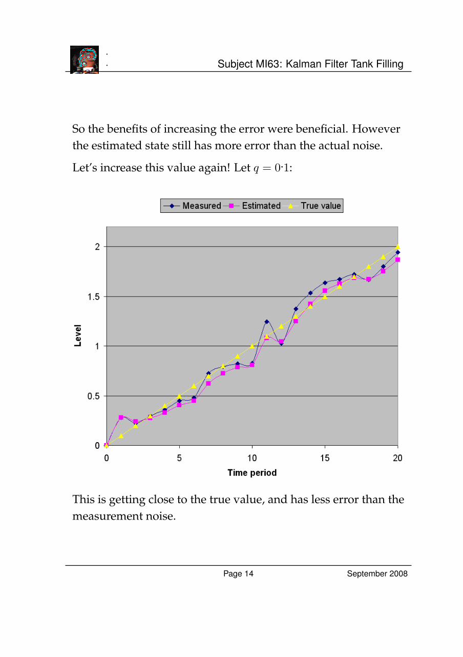
So the benefits of increasing the error were beneficial. Howeverthe estimated state still has more error than the actual noise.

Let’s increase this value again! Let q = 0.1:

This is getting close to the true value, and has less error than themeasurement noise.

September 2008

.


Let’s try q = 1 to see what happens:

Now there is almost no difference to the measured value. Thereis minor noise removal, but not much. There’s almost no pointin having the filter.

So what has been learnt here?

If you have a badly defined model, you will not get a goodestimate. But you can relax your model by increasing yourestimated error. This will let the Kalman filter rely more on themeasurement values, but still allow some noise removal.

In your own time, try playing with the measurement error r andsee what the effect is.

September 2008

.


Second Option: A Filling Model

2. Model the state process

To get better results, we need to change our Kalman model.

Let’s redefine it then.

So, the actual model is: Lt = Lt−1 + f

This translates to a continuous process transition of:

x = (xl, xf )>

A =

0 1

0 0

where xl is the level L, and xf = dxl

dt is the estimated filling rate,and A represents the tank continuously filling at rate xf(defined by f and the used time scale).

However, we want a discrete process. So A needs to be madetime-discrete. Just apply the infinite sum as given in MI37 (notethat Ai is zero in all four components, for all i > 1):

Ft =

1 ∆t

0 1

for all t ≥ 0. We will be ignoring B and u again.

September 2008

.


3. Model the measurement process

In this case, we can not measure the filling rate directly, but wewill still assume a noisy measurement of L. Therefore we have:

H = (1 , 0)

y = (y , 0)>

Indicating that there is no measurement for filling rate and thaty is the estimated measurement of xl.

4. Model the noise

The measurement process has not changed, so that means thatthe noise has not changed (i.e., R = r).

The process has changed, so we need to redefine the noise.

Now if we assume the noise is only in the filling part of theprocess, this would give us the continuous noise model with

Q =

0 0

0 qf

where qf is the filling noise.

Now, this continuous process can be approximated by atime-discrete process using:

Q(∆t) =∫ ∆t

0

eAτQeA>τdτ

September 2008

.


Using this continuous to discrete translation, we can take thecontinuous A and Q to approximate the discrete Q. This gives us(after some calculations - to be skipped here; again, apply theinfinite sum for the power of e):

Q =

∆t3qf

3∆t2qf

2∆t2qf

2 ∆tqf

For simplicity, we assume a continuous sampling rate of ∆t = 1.

Therefore,

Ft =

1 1

0 1

Q =

qf/3 qf/2

qf/2 qf

Also, the process is no longer scalar, so the covariance matrix is

P =

pl plf

plf pf

where the subscript denotes the relating variance and plf is thecovariance (which is symmetric, i.e., plf = pfl).

September 2008

.


5. Test the filter

The equations from Page 2 could be slightly simplified, but forour purposes, it is best just to put in the information from aboveinto the equations. (K can be simplified quite nicely.)

Predict:

x̂t|t−1 = Ftx̂t−1|t−1

Pt|t−1 = FtPt−1|t−1FTt + Qt

Update:

x̂t|t = x̂t|t−1 + Kt

(yt −Htx̂t|t−1

)Kt = Pt|t−1HT

t

(HtPt|t−1HT

t + Rt

)−1

Pt|t = (I−KtHt)Pt|t−1

This time we have an accurate model of a constant fill rate. Wewill assume that we have a noise of r = 0.1, and an accurateprocess noise of qf = 0.00001.

We have no idea of the initial state or filling rate, so we willmake x0 = (0 , 0)> with an initial variance of:

P0|0 =

1000 0

0 1000

We are assuming we have no idea of either values, and we areassuming that there is little or no correlation between thevalues.

September 2008

.


We will need to test these results under different conditions.The first test will be that the model is filling at a constant rate of0.1 per time frame, with an actual measurement noise of ±0.3.

If we plot this on a graph it looks as follows:

Notice that the filter quickly adapts to the true value. Note thatwe did not tell the Kalman filter anything about the actualfilling rate, and it figured it out all by itself. Even with a badunsure initialization.

Actually, if you give a Kalman filter a bad initialization, it takesthe first measurement as a “good” initialization.

September 2008

.


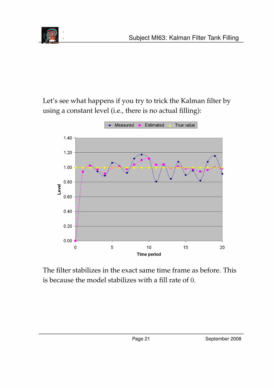
Let’s see what happens if you try to trick the Kalman filter byusing a constant level (i.e., there is no actual filling):

The filter stabilizes in the exact same time frame as before. Thisis because the model stabilizes with a fill rate of 0.

September 2008

.


Third Option: Constant, but Sloshing

Now let us test an extreme case. We will assume that the wateris at a constant level, but it is sloshing in the tank. This sloshingcan be modeled as a sine wave

L = c sin(2π r ∆t) + l

where c is an amplitude scaling factor, r is the cycle rate, and l isthe average level (as sin integrates to zero over time).

If we use c = 0.5, r = 0.05, and l = 1 we get the following result:

September 2008

.


There are two things you should notice about the Kalman filter:

1. The model is smoother than the noisy measurement, butthere is a lag behind the actual value. This is common whenfiltering a system that is not modelled correctly.

2. The amplitude of the filter is getting smaller and smaller.This is because the model is slowly converging to what itthinks is the truth... a constant level, which is accurate overtime.

If you wanted to model the sloshing properly, you would needto use an extended Kalman Filter, which also takes intoconsideration the non-linearity of the system.

See

www.cs.unc.edu/˜welch/kalman/media/pdf/kftool_

models.pdf

for details.

September 2008

.


Summary of the Three Tank Examples

The main points that you should learn from these examples are:

1. The model for your filter will try to fit the givenmeasurement data to the model you have provided. Thismay be undesirable. In the sloshing case, it may bedesirable to filter out the sloshing as “noise”, so you can getthe average level of the tank. If you wanted to measure thesloshing, then you need to model it.

2. The initialization and noise components of your filter doeffect the results of how the filter operates.

3. You need to think about the outcome of your filter; if youcan approximate that the time steps are small enough, thena simple linear model will work, but you will get lag.

September 2008

.


Coursework

63.1. Download the KalmanExample.xls spreadsheet from thecourse’s website.

Here there are two tabs, one for Options 1 and 2 (constant orwith filling), and one for Option 3 (constant and sloshing). Atab says the name of the model, followed by the name of theactual situation.

For each model, try changing the different noise parameters rand q to see the effect. Keep q static and change r, then viceversa.

Try changing the initialization values x0|0 and p0|0 to see theeffect on the overall outcome.

63.2. Go to the UNC (University of North Carolina) websitewith a dedicated Kalman filter learning tool:

www.cs.unc.edu/˜welch/kalman/kftool/index.html

Read the document describing the filter:

www.cs.unc.edu/˜welch/kalman/media/pdf/kftool_

models.pdf

Then play with the online Java tool. Once you have anunderstanding you can download the Matlab or Java code tosee how it operates.

September 2008

kalman filter applications - cornell university · kalman filter applications the kalman ﬁlter...

Documents